ument oom, -w,. () 36-412earch Laboratory of Electronics

aschusetts Institute of Technology-~~ ~ ~~, . ,, , , 1 _ , ...

A THEORY OF NONLINEAR SYSTEMS

AMAR G. BOSE

Lo?N

TECHNICAL REPORT 309

MAY 15, 1956

RESEARCH LABORATORY OF ELECTRONICSMASSACHUSETTS INSTITUTE OF TECHNOLOGY

CAMBRIDGE, MASSACHUSETTS

o Py

I~~~~~~i~I~bI.

I

: 2

.,oic, 44v A,I?:` : ·�ib 1(1Ib·,,·r·: a r··i�

·!c�

i ' ~, .

Iv

The Research Laboratory of Electronics is an interdepartmentallaboratory of the Department of Electrical Engineering and theDepartment of Physics.

The research reported in this document was made possible in partby support extended the Massachusetts Institute of Technology, Re-search Laboratory of Electronics, jointly by the U. S. Army (SignalCorps), the U. S. Navy (Office of Naval Research), and the U. S.Air Force (Office of Scientific Research, Air Research and Devel-opment Command), under Signal Corps Contract DA36-039-sc-64637, Department of the Army Task No. 3-99-06-108 and ProjectNo. 3-99-00-100.

II_ _ _ L I

MASSACHUSETTS INSTITUTE OF TECHNOLOGY

RESEARCH LABORATORY OF ELECTRONICS

Technical Report 309 May 15, 1956

A THEORY OF NONLINEAR SYSTEMS

Amar G. Bose

This report is based on a thesis submitted to the Department ofElectrical Engineering, M.I.T., May 14, 1956, in partial ful-fillment of the requirements for the degree of Doctor of Science.

Abstract

The Wiener theory of nonlinear system characterization is described and some of

its important concepts are discussed. Following these lines, a theory is developed for

the experimental determination of optimum time-invariant nonlinear systems. The

systems are optimum in a weighted mean-square sense in which the weighting function

is at our disposal.

The design of nonlinear systems is regarded as the problem of mapping the function

space of the past of the input onto a line that corresponds to the amplitude of the filter

output. By choosing a series expansion for this mapping operation that partitions the

function space into nonoverlapping cells, an orthogonal representation for nonlinear

systems is obtained that leads to convenient apparatus for the determination of optimum

systems. General methods are described for applying this theory to the determination

of systems that have a performance superior to that of given linear or nonlinear systems.

A criterion is established relative to which two systems are defined as "nearly equiva-

lent" and the approximation of nonlinear systems by linear and simple nonlinear systems

is discussed. The theory is extended to include the problem of multiple nonlinear pre-

diction and apparatus for the determination of optimum predictors is indicated.

IY ---·I�----I1�·�____*·^II I C II --_I - .--L

-· ---- I ��__

INTRODUCTION

A physically realizable nonlinear system, like a linear one, is a system whose

present output is a function of the past of its input. We can regard the system as a

computer that operates on the past of one time function to yield the present value of

another time function. Mathematically, we say that the system performs a transfor-

mation on the past of its input to yield its present output. When this transformation

is linear (the case of linear systems), we can take advantage of the familiar convolu-

tion integral to obtain the present output from the past of the input and the system is

then said to be characterized by its response to an impulse. That is, the response of

a linear system to an impulse is sufficient to determine its response to any input. When

the transformation is nonlinear, we no longer have a simple relation like the convolu-

tion integral, which relates the output to the past of the input, and the system can no

longer be characterized by its response to an impulse, since superposition does not

apply. Wiener has shown, however, that we can characterize a nonlinear system by

a set of coefficients and that these coefficients can be determined from a knowledge of

the response of the system to shot-noise excitation. Thus, shot noise occupies the same

position as a probe for investigating nonlinear systems that the impulse occupies as a

probe for investigating linear systems. The first section of this report is devoted to

the Wiener theory of nonlinear system characterization. Emphasis is placed on impor-

tant concepts of this theory that are used in succeeding sections to develop a theory for

the determination of optimum nonlinear systems.

I. THE WIENER THEORY OF NONLINEAR SYSTEM CHARACTERIZATION

AND SYNTHESIS

1.1 GENERAL REMARKS

The objectives of Wiener's method are: to obtain a set of coefficients which char-

acterizes a time-invariant nonlinear system, and to present a procedure for synthesizing

the system from a knowledge of its characterizing coefficients. An operator that relates

the output to the past of the input of a nonlinear system is defined in such a way that the

characterizing coefficients can be evaluated experimentally.

The method is confined to those nonlinear systems whose present behavior depends

less and less upon the remote past of the input as we push this past back in time. More

precisely, attention is restricted to those systems whose present output is influenced

to an arbitrarily small extent by that portion of the past of the input beyond some arbi-

trarily large but finite time. Furthermore, we shall restrict our attention to those

nonlinear systems that operate on continuous time functions to yield continuous time

functions. This is clearly no physical restriction, since physical time functions, though

they may change very rapidly, are continuous. The reasons for these restrictions will

become apparent in the development of the theory that follows.

1

�------ ·- II - -P· ------------*--�i��--·----·-Y---·r�---l� --I^-- ·-I I�--- - - �-- I -------- �----

According to Wiener, the most general probe for the investigation of nonlinear sys-

tems is gaussian noise with a flat power density spectrum, because there is a finite

probability that this noise will, at some time, approximate any given time function

arbitrarily closely over any finite time interval. Gaussian noise with a flat power

density spectrum can be approximated by the output of a shot-noise generator. Hence,

if two systems have the same response to shot noise, they will have the same response

for any input, and we say that the systems are equivalent. The Wiener theory of non-

linear system classification is based on this property of the shot-noise probe. A given

system is characterized by exciting it with shot noise and measuring certain averages

of products of its output with functions of the shot-noise input which can be generated in

the laboratory. The measured quantities are numerically equal to the coefficients in the

Wiener nonlinear operator. Once these coefficients are determined, a system can be

synthesized that yields the same response to shot noise as does the given system. Hence

the two systems are equivalent.

Recognizing that the present output of a nonlinear system is a function of the past of

its input, Wiener formulated his nonlinear operator by first characterizing the past of

the time function on which it operates by a set of coefficients and then expressing the

result of the operation (the system output) as an expansion of these coefficients (1). In

the development that follows we shall treat these problems separately; first the problem

of characterizing the past of a time function by a set of coefficients, and then the prob-

lem of expressing a nonlinear function of these coefficients.

1.2 DEFINITIONS

To simplify the description of the method, it is convenient at this point to define

certain quantities and relations.

A. The n t h Laguerre polynomial is defined (2) as

1 x d(n1) -Ln(x) = (n-l)' ed(nl) (x(n - l) ex) n =1,2,...

B. The normalized Laguerre functions hn(x) are defined as

Le- L(x) x 0O

hn(x) = (1)

0O x<O

The following orthogonality relation exists for these functions:

o 01 if m = n

hm(x) hn(x) dx = (2)0 if m n

2

"I � I I

I

C. The nth Hermite polynomial is defined (3) as

F (x) = ( 1)(n-) e (d)(n) = 1, 3,-x

D. The normalized Hermite polynomials n (x) are defined as

Fn(x)n(x) [2(n- 1)(nl) /Z/ ( 3)l/] /2

E. The normalized Hermite functions are defined as

x2/2n(X) = e in(X)(4)

These functions form a normal orthogonal set over the interval -oo to oo. Conse-

quently, we have the relation

co 0 i-2 i m=n

lm(X) ln(x) e -x dx (5)moo tno m n

1.3 CHARACTERIZING THE PAST OF A TIME FUNCTION

Given a time function x(t), our object is to determine a set of coefficients that

characterize its past. The coefficients are said to characterize the past of x(t) if we

can construct this past from a knowledge of them. Let us confine our attention here

to real time functions x(t) that have the property

x2 (t) dt < 0

The past of such time functions can be expanded in a complete set of orthogonal

functions. Furthermore, from a knowledge of the coefficients of this expansion, we

can construct the time function almost everywhere (4). Because of their realization

as the impulse response of rather simple networks, Wiener chose to expand the past

of x(t) in terms of Laguerre functions. These functions form a complete set over the

interval 0 to oo and have the orthogonality property indicated in Eq. 2. The expansion

of the past of x(t) in terms of the Laguerre functions is

o00

x(-t) = un hn(t) t > O (6)

n=l

where the present time is t = 0 and the un are the Laguerre coefficients of the past of

x(t). Taking advantage of the orthogonality property of Eq. 2, we obtain the following

3

_ I I I_ - - --L_�_. -�··II---- ---- - ··--- ·I - - ·

OUTPUTTERMINAL I - I' n-n' (S- I-(S- -S'

PAIRS

Fig. 1. Laguerre network. For R = L = C = 1, the impulse response

at the nth-output terminal pair is given by Eq. 1.

INPUT LAGUERRE NETWORK OUTPUTx(t) IMPULSE RESPONSE IS rt)

hn(t)

Fig. 2. Block diagram of Laguerre network showing n t h output.

expression for the u .

u = x(-t) h (t) dt (7)

These Laguerre coefficients are readily generated, in practice, as the outputs of

a rather simple network whose input is x(t). This network, shown in Fig. 1, is called

a Laguerre network. It is a constant-impedance, lossless, ladder structure, terminated

in its characteristic impedance, and preceded by a series inductance. For a detailed

description of Laguerre networks, their analysis and synthesis, see reference 2. For

our purposes, it is sufficient to know that the impulse response of the Laguerre network

at the nth-output terminal pair on open circuit is h (t) for n = 1, 2, 3,... We must now

show that if x(t) is applied to the input of this network, the output at the nth terminal pair

at time t = 0 is the n t h Laguerre coefficient un of the past of x(t) up to the time t = O0. To

this end, we consider the block diagram of the Laguerre network shown in Fig. 2. For

simplicity, only the nth-output terminal is shown. The network input is x(t). Its output

rn(t) is given by the convolution of x(t) with hn(t). That is,

rn(t) = x (t-T) hn(T) d T

At time t = 0, the output is

rn() = X(-T) h n(T)dT (8)

But the right side of this equation is seen to be equivalent to the expression for

un that is given in Eq. 7. Hence we see that if x(t) is applied to the input of a Laguerre

4

_ _

network, the output of the nt h terminal pair at time t = 0 is equal to the n t h Laguerre

coefficient of the past of x(t) up to the time t = 0. In general, the output of the nth ter-

minal pair of the Laguerre network at any time t is equal to the n t h Laguerre coefficient

of the past of the input up to the time t.

1.4 PROPERTIES OF THE LAGUERRE COEFFICIENTS OF A SHOT-NOISE PROCESS

Since the probe for the investigation of nonlinear systems in the Wiener theory is

shot noise, it will be necessary in our development of this theory to make use of several

properties of the Laguerre coefficients of a shot-noise process.

When the input of a Laguerre network is shot noise, the outputs (the Laguerre coef-

ficients of the past of the shot-noise input) have the following three properties that are

of interest:

1. They are gaussianly distributed.

2. They are statistically independent.

3. They all have the same variance.

The first property follows from the well-known result that the response of a linear

system to a gaussian input is gaussian (5) (recall that shot noise is a gaussian time

function with a flat power density spectrum).

The second property is proved as follows. Consider the Laguerre functions hm(t)

and hn(t). Let Hm(w) and Hn () be the Fourier transforms of h (t) and h (t), respec-

tively. Then H (w) and H (co) are the transfer functions from the input of the Laguerreth th

network to the m - and n -output terminal pairs. The cross-power density spectrum

nm(w) of the mth- and nth-output time functions can be expressed as

nm( ) = Hm(o) Hn() ii( tU) (9)

where ii(o) is the input power density spectrum and the star denotes the complex con-

jugate of H n() (6). The crosscorrelation function bnm(T) of these output time functions

is given by the Fourier transform of nm(o) as follows:nm

~nm(T) = fn(t) fm(t+T) = J ~nm() eJT d (10)

in which the bar indicates averaging with respect to time. By the use of Eq. 9, Eq. 10

becomes

nm(0) = fn(t) f(t) = H() Hn(o) ii() dw (11)

for T = 0

If .ii( () is a constant, then Eq. 11 can be written1.1

5

� _j�r --- _I II I - -·X

00oo

~nm(o) = fn(t) fm(t) = mii() H) H(W) d (12)

We now make use of the Parseval theorem to express the integral in Eq. 12 as follows:

CI oo

r . Hm() H (o) d = ( hn (t) dt (13)

Using the orthogonality property of the Laguerre functions (Eq. 2) in Eqs. 13 and 12,

we obtain

ZTrii(o) m n

fn(t) fm(t) = (14)

0 m n

when ii (w) is a constant. Note that if ii (w) is a constant, it can have no impulse at the

origin and thus the input and output time functions of the Laguerre network must have

zero means. Therefore, we have shown that the outputs of the Laguerre network are

linearly independent when the power density spectrum of the input is flat. (Note that

this is true whether or not the input time function is gaussian and that it also holds for

any orthogonal set of networks, not only for the Laguerre network.)

In the case of a shot-noise input, the Laguerre coefficients are gaussian time func-

tions (property 1), and linear independence implies statistical independence; thus

property 2 is proved.

Property 3 can be proved by solving for the variance of the n t h Laguerre coefficient

in terms of the power density spectrum of the nth output of the network. However, it

can be seen very simply by recalling that the Laguerre network, except for its first

series inductance, is a constant-resistance, lossless structure terminated in its char-

acteristic resistance. If, in Fig. 1, we look to the right at any of the output terminal

pairs n-n, we see the characteristic resistance of the network. Since the structure is

lossless, the same power flows through each section and, since the impedance at each

section is resistive and the same for each section, the mean-square value of every

Laguerre coefficient is the same. For a shot-noise input, the mean value of each coef-

ficient is zero. Hence the variance an = un(t) - un(t) is the same for all Laguerre

coefficients. In particular, if the level of the shot-noise input to the network of Fig. 1

is properly adjusted, all the Laguerre coefficients will have -r2 = 1. In the development

of the Wiener theory that follows we shall assume this to be the case.

In section 1.3 we restricted our attention to time functions that are square integrable

over the interval -oo to oo. In the present section we speak of applying shot noise to the

input of the Laguerre network. This is justified by the fact that the past of any physical

time function which we can generate as an input to our Laguerre network is square inte-

grable, since it starts at some time in the finite past.

6

Any practical application of the Wiener theory must, of course, use only a finite

number of Laguerre coefficients to characterize the past of the system input. Since

all the Laguerre functions decay exponentially (Eq. 1), for any finite number of these

functions there exists some time in the finite past such that the present outputs of the

Laguerre network are influenced to an arbitrarily small extent by the behavior of the

input prior to this time. That is, for all practical purposes, the outputs of the Laguerre

network are not cognizant of the past of the input beyond some finite time. Hence, as

we mentioned in section 1.1, the application of the Wiener theory is restricted to sys-

tems whose present output is influenced to an arbitrarily small extent by that portion

of the past of the input beyond some arbitrarily large but finite time.

1.5 WIENER NONLINEAR OPERATOR

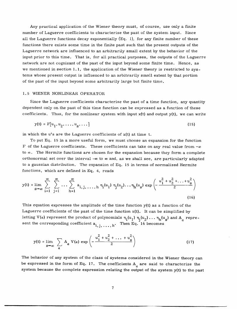
Since the Laguerre coefficients characterize the past of a time function, any quantity

dependent only on. the past of this time function can be expressed as a function of these

coefficients. Thus, for the nonlinear system with input x(t) and output y(t), we can write

y(t) = F[u1 , U 2 . . .Us .] (15)

in which the u's are the Laguerre coefficients of x(t) at time t.

To put Eq. 15 in a more useful form, we must choose an expansion for the function

F of the Laguerre coefficients. These coefficients can take on any real value from -oo

to oo. The Hermite functions are chosen for the expansion because they form a complete

orthonormal set over the interval -oo to oo and, as we shall see, are particularly adapted

to a gaussian distribution. The expansion of Eq. 15 in terms of normalized Hermite

functions, which are defined in Eq. 4, reads

yo 00 0t ) + li + y(t) = lim ' a. ... a . h ¶1i(u1 ) inj(u 2 ).. rlh(Us) exp z 2 s

i=1 j=l h=l1

(16)

This equation expresses the amplitude of the time function y(t) as a function of the

Laguerre coefficients of the past of the time function x(t). It can be simplified by

letting V(a) represent the product of polynomials i(ul) j(u2) ... Ih(us) and A a repre-

sent the corresponding coefficient a h Then Eq. 16 becomes

u + 2 + u + usy(t) = limr A a V(a) exp - ) (17)

a

The behavior of any system of the class of systems considered in the Wiener theory can

be expressed in the form of Eq. 17. The coefficients A are said to characterize thea

system because the complete expression relating the output of the system y(t) to the past

7

2_ ·L- I -I - ---- · ILe- ----- I- __ ----

of its input x(t), for any input time function, is known when the A are known.

We now come to the problem of characterizing a given nonlinear system, that is,

the problem of evaluating the Aa that correspond to a given nonlinear system. The

object is to obtain an expression for the A suitable for experimental evaluation. To

obtain such an expression, Wiener multiplies both sides of Eq. 17 by V(p) and then

makes use of the gaussian distribution of the Laguerre coefficients of a shot-noise

process to obtain Eq. 26 for the A . However, we shall use a different approach in

order to arrive at Eq. 26 that will give us a better physical understanding of the Wiener

method.

In the practical case, we shall always use a finite number of Laguerre coefficients

and Hermite functions. Then the sum on the right side of Eq. 17 does not yield y(t)

exactly but only approximates it. We can regard the finite sum

U+ u 2Aa V(a) exp - (18)

a

as representing the output of a nonlinear system in terms of s Laguerre coefficients

of its input and a finite number of Hermite functions. We want to choose the A so that

this sum best approximates the output y(t) of the given system with respect to some

error criterion when both systems have the same input. Since, according to section 1.1,

the most general time function is shot noise, we shall let it be the common input. We

define

2TV lim -A exp a V(a exp 2 dtT-oo

(19)

as the error between the outputs of the two systems. The justification of the choice of

this weighted mean square error is that it leads to convenient independent expressions

for the Aa, as we shall see. We now minimize with respect to the A . In particular,

for the coefficient Ap, we have

T (2 U2+' u(3 e1 Tu

lim 2T Z V(P) y(t)- A V(a) exp dt (20)T--oo La 2

For the error to be a minimum with respect to Ap, we must set Eq. 20 to zero. This

gives

lim T T y(t) V() dt = lim 2T P V(pd) V() exp ( dt

T-~oc ."-T T~-oo 2T J..T LA ep-/

(21)

8

__ __

We have seen (sec. 1.4) that the Laguerre coefficients of the past of a shot-noise

process are statistically independent, normalized, gaussian variables. Thus the

joint distribution of the Laguerre coefficients is

(2w)S/ exp + u + usP(u 1 .... u s ) = 2-s/ exp ) (22)

Our knowledge of this distribution is helpful in evaluating the integral on the right

side of Eq. 21. Taking advantage of the ergodic theorem, we can replace the time

average of the right side of Eq. 21 by the corresponding ensemble average, with the

result:

T

lim T-oc T

y(t) V(P) dt =

00

... scIUl + ... + \

V() Aa V(a) exp - Z

a

X P(u ... S) du1... du

After using Eq. 22 in Eq. 23 and interchanging the order of integration and

we obtain

summation,

V(a) V(f) exp (-u+ + u) du ... dus(Zr) s / 2 y(t) V(3) = E Aa a°a

(24)

in which the bar above y(t) V(p) indicates the time average of this quantity. Since

V(a) and V(^) are products of Hermite polynomials of the Laguerre coefficients, we

can separate Eq. 24 into a product of integrals each of which involves only one Laguerre

coefficient, as in the following equation:

(2s) s / 2 y(t) V(P)

o0

ZA 2 00oo

1.-u ..*i(Ul) *i, (U1) e du 1 ...

2

h(Us) -lh,(Us) e S du s

In this equation the unprimed subscript indices belong to those Hermite polynomials

that make up V(a), while the primed indices belong to those Hermite polynomials that

make up V(p). If we recall the orthogonality property of the Hermite functions (Eq. 5),

it is clear that unless all the primed indices i', j', . . ., h' in Eq. 25 are equal to the

corresponding unprimed indices i, j, ... , h, in other words, unless equals a, at

least one of the integrals will be zero. By the same token, if = a, then all the inte-

grals have the value unity. Hence Eq. 25 reduces to

9

(23)

(25)

I _ _I _ � �1 �1_1 II_1ILI____III_�__-· _I-�_- IIII I _ _ III I II ··__I I I

00~

(2r)s/2 y(t) V(p) = Ap (6)

which provides the basis for the experimental determination of the characterizing

coefficients A . The reason for the choice of Hermite functions to expand the rightaside of Eq. 15 now becomes apparent. The joint gaussian probability density of the

Laguerre coefficients of the shot-noise input (Eq. 22) supplies the necessary exponen-

tial weighting factor in Eq. 23, thus enabling us to take advantage of the orthogonality

of the Hermite functions in evaluating the coefficients A .

This approach to the Wiener theory clearly points out that, for any given number

of Laguerre coefficients and Hermite functions, this theory determines that system

whose output best approximates (in the weighted mean-square sense of Eq. 19) the

output of the given system for shot-noise input of both systems. As the number of

Laguerre coefficients and Hermite functions is increased, the output (for shot-noise

input) of any system of the Wiener class of systems can be approximated with vanishing

error. And, from the discussion of section 1.1, if two systems have the same response

to shot noise, then they have the same response to any common input and can be con-

sidered equivalent.

1.6 EXPERIMENTAL APPARATUS FOR CHARACTERIZING AND

SYNTHESIZING NONLINEAR SYSTEMS

Equation 26 provides the basis for the experimental determination of the charac-

terizing coefficients A . The apparatus for the determination of the coefficients A

is shown in Fig. 3. The output of a shot-noise generator is fed simultaneously into the

given nonlinear system and into the Laguerre network. The output of the given

nonlinear system is y(t). The outputs of the Laguerre network are fed into a device

involving multipliers and adders. This device generates products of Hermite poly-

nomials (the V's) whose arguments are the Laguerre coefficients. Each output of this

Hermite polynomial generator, when multiplied by y(t) and averaged, yields, by Eq. 26,

one of the characterizing coefficients of the given nonlinear system.

Having described the method for determining the characterizing coefficients of a

nonlinear system, we now turn our attention to the Wiener method of synthesis of non-

linear systems from their characterizing coefficients. The general representation of

Fig. 3. Block diagram of the circuitry for the characterization of nonlinear systems.

10

Fig. 4. Block diagram of the circuitry for the synthesisof nonlinear systems.

a nonlinear system is given by Eq. 17, which is the guide for the synthesis problem.

This equation tells us that, for each a, we must generate V(a) and multiply it by Aa

and exp [-(u + ... + u)/2 . Then each product must be added to give the system out-a 1 Js

put y(t). In practice, the number of multipliers is reduced if we first form the sum of

the products AaV(a) and then multiply by the exponential function.

The exponential function, exp [- (u + ... + )/ can be obtained as the product

of s exponential function generators whose inputs are u through us. Such generators

give an output of exp(-uZ/Z) when the input is u. They are realizable, among other

ways, in the form of a small cathode-ray tube with a special target which generates

the exp(-u2/Z) function.

The block diagram of the apparatus for the synthesis procedure is shown in Fig. 4.

EXAMPLE 1. In order to fix ideas, let us consider a simple example which is

particularly suited to characterization and synthesis by the Wiener method. It should

be emphasized that the Wiener method is an experimental method and that, for the pur-

pose of illustrating mathematically how the method works, only the simplest of examples

can be handled analytically. Let the example be a nonlinear system that contains no

storage elements. Furthermore, let its output-input characteristic (transfer charac-

teristic) be given by the equation

y(t) = exp(-x 2 (t)/Z) (27)

In both the characterization and synthesis procedures that have been described, the

function of the Laguerre network is to introduce dependence of the system output on the

past of its input. The nonlinearity is brought about by the Hermite polynomial generator.

For this simple example, there is no dependence upon the past and thus we can by-pass

the Laguerre network. In the experimental procedure, the fact that this given nonlinear

system has no storage could be determined from the results of a priori tests made on

the system.

We notice that, as a result of by-passing the Laguerre network, the variables u

through us (Fig. 3) are replaced by the single variable x(t), as shown in Fig. 5. Equa-

tion 16 then becomes:

y(t) = ai qi(x) exp(-x2 /2) (28)

i

11

I I _ I_ I�_I _1_ 1�1__�11� 1_ ___ __I_

Fig. 5. Block diagram of the circuitry forof no-storage nonlinear systems.

the characterization

2()

(a)

xt(t)

x(t) FUNCTION y(t= e GENERATOR

xt

e 2

(b)

Fig. 6. (a) Synthesis of the nonlinear characteristic y =accordance with the general procedure of Fig. 4.reduced form of part (a).

exp(-x 2 /2) in(b) Equivalent

and Eq. 26 becomes:

a i = (21)1/2 y(t) 1i(x)

Let us make use of the ergodic theorem to evaluate this time average as an ensemble

average. Using Eq. 27, we can write

o00

a i = (2r)l/2 i~~~~s

ri(x) exp(-x2/2) P(x) dx

But since, in the test circuits (Fig. 5), x(t) is the output of an ideal shot-effect gener-

ator, the probability density of x is

P(x) = (21r)- 1 /2 exp(-x 2 /2) (31)

Thus

12

(29)

(30)

�

2a i= f i(x)e dx (32)

Referring to Eq. 3 and the definition of the Hermite polynomial, we see that

1 () = - 1/4 (33)

With this result, Eq. 32 can be written

a = 1 / 4 hi(x) nl(x) ex dx (34)

As a consequence of the orthogonality of the Hermite functions (Eq. 5), we have

1/41

a i = i 1 (35)

These coefficients serve to characterize the simple nonlinear system of this example.

Now let us synthesize the system from these coefficients. The guide for the syn-

thesis is Eq. 28, which corresponds to Eq. 17 for the more complicated case involving

storage. Since, from Eq. 35, only one coefficient is different from zero, the sum in

Eq. 28 has only one term and can be written

y(t) = a (x) exp(-x2/2) (36)

The synthesis of the system amounts to generating rl 1(x) and exp(-x2/2) and forming

the product indicated in Eq. 36. The formal synthesis of the system, in accordance

with the block diagram of Fig. 4, is shown in Fig. 6a. Since 11 (x) is just a constant,independent of x, the system is seen to be equivalent to that of Fig. 6b. We see that,

for example 1, the synthesized system consists solely of the "function generator," a

component which in the more complicated case will form only a part of the synthesized

system.

1.7 OBSERVATIONS AND COMMENTS

It can be seen from Eq. 16 that if we choose to represent the past of the system

input by s Laguerre coefficients and if, furthermore, we decide to let the Hermite

polynomial indices, i,j,...,h (Eq. 16), range from 1 to n, we have n s coefficients

A to evaluate. Without a doubt this number can become quite large in many cases

of practical interest. However, with the freedom that exists in nonlinear systems we

can hardly expect to apply such a general approach without a great deal of effort. At

present, the large number of multipliers that is required for the generation of the Her-

mite polynomials and their products is the principal deterrent to the practical application

13

�____II� I_ _ _ _ C ____ _ _ _I �

of the Wiener method of characterization and synthesis. It is safe to say that, at

present, the Wiener theory is of greater theoretical than practical interest.

One of the most significant contributions of the Wiener theory is that it shows us

that any nonlinear system, of the broad class of systems considered by this theory,

can be synthesized as a linear network with multiple outputs cascaded with a nonlinear

circuit that has no memory of the past (Fig. 4). The linear network (the Laguerre

network) serves to characterize the past of the input and the nonlinear no-storage

circuit performs a nonlinear operation on the present outputs of the linear network

to yield the system output. Thus, regardless of how the linear and nonlinear operations

occur in any given circuit, the same over-all operation can be achieved by a linear

operation followed by a nonlinear one, as shown in Fig. 4.

Another important contribution of the Wiener theory is the concept of the shot-noise

probe for a nonlinear system. Just as the response of a linear system to an impulse is

sufficient to characterize the system, so Wiener has shown that the response of a non-

linear system to shot noise is sufficient to characterize it.

In the Wiener theory two parameters remain free: the time-scale factor of the

Laguerre functions and the scale factor in the argument of the Hermite functions. For

convenience, both have been taken as unity in the preceding development. We may

choose these as we desire in order to reduce the apparatus that is necessary for per-

forming a given operation. Unfortunately, we have no simple procedure for determining

the optimum values of these scale factors to enable us to do the best job with a given

number of Laguerre coefficients and Hermite functions. We shall see a possible

approach to this problem when we discuss a similar but somewhat simpler problem

that arises in connection with the determination of optimum filters by the theory devel-

oped in the following sections.

Since linear systems form such an important class of systems in engineering, it is

proper that we ask of any nonlinear theory, "How conveniently does this theory handle

linear and nearly linear systems? " Although the Wiener theory includes within its

scope linear as well as nonlinear systems, it is not particularly suited for application

to the former. The reason for this can be seen by observing the form of the general

Wiener system (Fig. 4). We note that the exponential function generator by-passes the

Hermite polynomial generator. In order for the system of Fig. 4 to represent a linear

system, the operation from the output of the Laguerre network to the output of the sys-

tem must be linear. This means that the gain coefficients A must have values that

cause cancellation of the output of the exponential function generator and give the desired

linear operation on the Laguerre coefficients. To achieve this cancellation effect, a

very large number of Hermite functions will generally be required and, even then, we

may have the unfavorable situation of obtaining a desired output that is the small dif-

ference of two large quantities. The nonlinear theory that is developed in the following

sections does not suffer from this difficulty and, as we shall see, can be readily applied

to linear and nearly linear systems, as well as to general nonlinear systems.

14

___

II. THE FILTER PROBLEM

2.1 OBJECTIVES AND ASSUMPTIONS

We have seen how we can synthesize general nonlinear systems from a knowledgeof their characterizing coefficients. We now turn our attention to the problem of deter-

mining optimum nonlinear systems or filters.

We shall deal with time-invariant nonlinear systems that operate on statistically

stationary time functions. The filter problem considered here is one of determiningthat system, of a class of systems, that operates on the past of a given input time func-tion x(t) to yield an output y(t) that best approximates a given desired output z(t) withrespect to some error criterion. Wiener has shown that when the optimum filter ischosen from the class of linear systems, and when the mean-square-error criterionis adopted, this optimum filter is determined by the autocorrelation function of the inputtime function and the crosscorrelation function of the input with the desired output (7).Since these correlation functions determine the optimum mean-square linear filter, thesame linear filter is optimum for all time functions that have these same correlationfunctions in spite of the fact that other statistical parameters of these time functionsmay be very different. It is in the search for better filters that we turn to nonlinearfilters which make use of more statistical data than just first-order correlation

functions.

As Zadeh (8) pointed out, there have been two distinct modes of approach to the

optimum nonlinear filter problem. One approach parallels the approach of Wiener tolinear systems by choosing the form or class of filters and then finding the optimummember of this class by minimizing the mean square error between the desired outputand the actual system output. The other approach formulates an appropriate statisticalcriterion and then determines the optimum filter for this criterion with little or norestrictions upon the form of the filter. Both of these approaches yield equations foroptimum filters in terms of higher-order statistics (higher-order distribution functionsor correlation functions) of the input and desired output. In applying these approaches

we are, in general, faced with two problems. First, we must obtain the necessarystatistical data about the input and desired output and then we must solve the design

equations, which usually are quite complex, for the optimum filter in terms of thesedata. In nonlinear filter problems we find that the amount of statistical data that arerequired in the design of the filter-usually far exceeds the available data and we findit necessary to make certain simplifying assumptions or models of the signal and noiseprocesses in order to calculate the required distributions.

Instead of assuming a statistical knowledge of the filter input and desired output,the approach to the nonlinear filter problem developed in this work assumes that wehave at our disposal an ensemble member of the filter-input time function x(t) and the

corresponding ensemble member of the desired filter output z(t). By recording ormaking direct use of a portion of the given filter-input time function, we obtain the

15

ensemble member of x(t). The ensemble member of z(t) can be determined in different

ways, depending upon the problem. For pure prediction problems z(t) is obtained

directly from x(t) by a time shift. For filter problems involving the separation of sig-

nal from noise at the receiver in a communication link, we can, in the program for the

design of the filter, record a portion of the desired signal z(t) at the transmitter and

the corresponding portion of x(t) at the receiver. For the radar type of problem, in the

program for the design of the filter, z(t) can be generated corresponding to signals

x(t) received from known typical targets.

Since the ensembles of x(t) and z(t) contain all the statistical information concerning

the filter input and desired output, and since we shall make direct use of these time

functions in our filter determination, it is not necessary to make any assumptions about

the distributions of x(t) and z(t). Thus, for example, in the problem of designing a filter

to separate signal from noise, we need make no assumptions about the statistics of the

signal or noise, or about how the two are mixed.

We note that, in most practical cases, our assumption of knowing a portion of x(t)

and z(t) does not restrict us any more than the usual assumptions of knowing the higher-

order probability densities of the input and desired output do; for at present, except in

very simple cases, the only practical way of obtaining these statistics is to measure

them from ensembles of x(t) and z(t) when these ensembles are available. When they

are available, the present approach makes measurements on them that yield optimum

filters directly, instead of first measuring the distributions and then solving design

equations in terms of these measured values.

2. 2 RELATION TO THE CHARACTERIZATION PROBLEM

The Wiener theory of nonlinear system characterization and synthesis provides us

with a physically realizable operator on the past of a time function that includes within

its scope a very large class of nonlinear systems. Consequently, we shall investigate

the possibility of determining the optimum nonlinear filter (for a given task and a par-

ticular error criterion) from the class of systems of the Wiener theory.

Figure 3 shows the experimental procedure for obtaining the characterizing coef-

ficients for a given nonlinear system (the system labeled "Nonlinear System Under

Test"). Notice that the A are completely determined from a knowledge of the response

of the given system to a shot-noise input. In fact, the presence of this system is not

necessary in the experimental procedure of Fig. 3 if we have recordings of an ensemble

member of the shot-noise input x(t) and the corresponding output y(t). By feeding the

recording of x(t) into the Laguerre network and the recording of y(t) into the product-

averaging device, in place of the output of the given system we obtain the A a that cor-

respond to the given system; that is, we obtain the A that correspond to the system

which operates on the shot noise x(t) to yield y(t). This arouses our curiosity con-

cerning the possibility of determining the A for the optimum filter problem directly

from a knowledge of an ensemble member of its input and its desired output time

16

x(t) LAGUERRE U2 HERMITE VCA~ =~POLYNOMIAL

GENERATOR

z(t) DUCT s0 * AVERAGING (21r)

2A = Z (t)V(,)

DEVICE

Fig. 7. Block diagram of experimental apparatus for the determination of anoptimum filter when the given filter input x(t) is shot noise. z(t) isthe desired filter output.

functions without actually having the filter at our disposal. To this end, let us consider

the optimum filter problem and see how it differs from the characterization problem

discussed above.

Unlike the characterization problem, in the determination of an optimum filter we

do not have at our disposal the system labeled "Nonlinear System Under Test" in Fig. 3.

In the filter problem this system would be the optimum filter - exactly what we are

searching for. Consider the following problem. Suppose that we want to find a non-

linear filter whose input is a white gaussian time function x(t) and whose desired output

is the stationary random time function z(t). Suppose also that we have at our disposal

an ensemble member of x(t) and the corresponding ensemble member of z(t). We excite

the Laguerre network of Fig. 3 with x(t) and feed z(t) into the product-averaging device

in place of y(t), as shown in Fig. 7. From the discussion above, it is clear that if the

desired filter, which operates on x(t) to yield z(t), is a member of the class of systems

considered in the Wiener theory, the test procedure of Fig. 7 will yield the A that

correspond to this system. We can then synthesize it in the general form shown in

Fig. 4. However, it will usually happen that the desired system is not even physically

realizable, let alone a member of the Wiener class of nonlinear systems. In this case

the derivation of section 1.5 shows that the procedure indicated in Fig. 7 will yield that

system of the Wiener class (with as many Laguerre coefficients and Hermite functions

as are used in the test apparatus) whose output best approximates z(t) in a weighted

mean-square sense. Thus, for the special case of white gaussian filter input, we can

adapt the Wiener method of characterization to the experimental determination of opti-

mum nonlinear filters.

2.3 NEED FOR A GENERAL ORTHOGONAL REPRESENTATION

When the given filter input is not shot noise we can no longer apply the method

described above to determine the optimum filter. Recall that the orthogonality relations

that led to Eq. 26 for the A depended upon the fact that the Laguerre coefficients were

gaussianly distributed and statistically independent, and this fact, in turn, depended on

the fact that the input of the Laguerre network was shot noise. When x(t) is not shot

noise we no longer obtain independent relations (Eq. 26) for the A and the procedure

17

_ _ _ ._ --- --

for determining them (Fig. 7) is no longer valid. Thus we appreciate the need of an

expression for a nonlinear operator in which the terms in its series representation are

orthogonal in time, irrespective of the nature of the input time function. The develop-

ment and application of such an operator is the subject of the following sections.

III. OPTIMUM NONLINEAR FILTERS

3.1 OBJECTIVES

We shall develop an orthogonal representation for nonlinear systems that enables

the convenient determination of optimum nonlinear filters. The development is best

described if, before proceeding to the general filter, we first examine the class of

no-storage nonlinear filters.

3.2 NO-STORAGE NONLINEAR FILTER

By a no-storage system we mean one whose output, at any instant, is a unique func-

tion of the value of its input at the same instant. We call the input-output characteristic

of this system the transfer characteristic.

Let x(t) and z(t) be the given filter-input and desired filter-output time functions,

respectively. We assume that x(t) and z(t) are bounded, continuous time functions.

This is clearly no restriction in the practical case and it enables us to confine our

attention to approximating desired filter transfer characteristics that are bounded and

continuous. Since x(t) is bounded, there exists an a and b which are such that

a < x(t) b for all t. Now consider a set of n functions j(x) (j = 1. n) over the

interval (a,b). These functions are defined as follows:

w W

1 for xj 2-x < xj + 2-, j ( 1 . n-

W nand x - x b, j = n (37)

J!~ 2 ~~x. =a+wj 0 for all other x J

A plot of the jth function of this set of functions is shown in Fig. 8. [A separate

b-a

i= o

()i

-- ---- --- -- ]0 o . . b a

Fig. 8. Gate function j (x).

18

I

definition is given for n(x) in order to include the point b. In practical application we

simply generate n functions of equal width that cover the interval (a, b). ] Clearly, thisset of functions is normal and orthogonal over the interval (a, b). We shall refer to these

functions as "gate functions." Let us define y as a gate-function expansion of x,

n

y = aj j(X) (38)j=1

It is clear that by taking n sufficiently large y can be made to approximate any single-

valued continuous function of x arbitrarily closely everywhere on the interval (a, b).

When x is a function of time it is convenient to write Eq. 38 as

n

y(t) = aj cj[x(t)] (39)j=l

As a consequence of the nonoverlapping property of the gate functions along the x-axis,

the j[x(t)] will, for any single-valued time function x(t), form an orthogonal set in time,

as well as an orthonormal set in x. Furthermore, this time-domain orthogonality holds

for any bounded weighting function G(t). That is,

jO i k

G(t) j[x(t)] k[x(t)] = G(t) [x(t)] j k (40)[1X) j = k

Relation 39 specifies the form of an equation that defines a no-storage nonlinear

system. The determination of an optimum no-storage filter for a given error criterion

consists of choosing the a in such a manner that, for a given x(t), the error between

y(t) and the desired output z(t) is a minimum. We adopt a weighted mean-square-error

criterion in which G(t) is, as we shall discuss later, a non-negative weighting function

at our disposal. More specifically, we minimize the error

= lim T G(t) 5(t) aj j[x(t)] dt (41)T-oo

with respect to the n-coefficients aj. Differentiating with respect to ak and setting theresult to zero, we obtain

= lim Z T - ZG(t) +k[x(t)] {z(t) - E aj jt = 0 (42)a k T-oo th o a .

where k = (1, ... ,n). If we denote the operation of time-averaging by a bar over the

19

-�--1_-------·1�-·1�.� _�1_.� ·--- �yl I�-_I� I

averaged variable, Eq. 42 can be written as

n

G(t) qk[x(t)] E aj bj[x(t)] = z(t) G(t) qk[x(t)] (43)j=l

If we make use of the time-domain orthogonality of the gate functions in Eq. 40, Eq. 43

reduces to

ak G(t) k[x(t)] = z(t) G(t) ,k[x(t)] (44)

It follows from the definition of the j(x) given in Eq. 37 that [x(t)] = j[x(t)], so that

Eq. 44 is equivalent to the equation

ak G(t) k[x(t)] = z(t) G(t) qk[x(t)] (45)

This equation provides a convenient experimental means of determining the desired

coefficients ak. The experimental procedure for the evaluation of these coefficients is

shown in Fig. 9. An ensemble member of x(t) is fed into a level-selector circuit and

the corresponding ensemble member of z(t) is fed into the product-averaging device.

The output of the level-selector circuit is unity whenever the amplitude of x(t) falls

within the interval of the ktM gate function and zero at all other times. This output is

used to gate the weighting function G(t). The output of the gate circuit is then averaged

and also multiplied by z(t) and averaged to yield the two quantities necessary for deter-

mining ak in Eq. 45.

From a knowledge of the ak we can directly construct a stepwise approximation,

like that of Fig. 10, to the desired optimum transfer characteristic (see Eq. 38). The

synthesis of the filter can be carried out formally in accordance with Eq. 38 by using

level-selector circuits and an adder, as shown in Fig. 11, or we can synthesize the

optimum characteristic by any of the other available techniques, such as piecewise-

linear approximations or function generators.

In order to become more familiar with the operation and terminology of this method,

let us consider a very simple example. We shall do analytically what, in practice, the

experimental procedure that is indicated in Fig. 9 does for us.

EXAMPLE 2. Suppose we are given an ensemble member of x(t) and the corre-

sponding ensemble member of z(t). Furthermore, suppose that the desired filter output

z(t) is equal to f[x(t)], where f is a continuous real function of x. We desire to verify

the fact that the filter determined by the procedure indicated in Fig. 9 is actually a

stepwise approximation to the transfer characteristic f(x). For simplicity, let us

assume that n has been chosen sufficiently large so that the function f(x) is approxi-

mately constant over the width of the gate functions and let us choose G(t) equal to a

constant so that the conventional mean-square-error criterion will result. For these

conditions, whenever k[x(t)] has a nonzero value, x must lie in the interval of width w

20

WEIGHTINGFUNCTION (t)

GIVEN FILTER (x) GENERATOR iGATE G(t) (x) AVERAGING

CIRCUIT)UT

DESIRED FILTER PRODUCTOUTPUT z (t) AVERAGING z(t)Gt)kx)

CIRCUIT

Fig. 9. Experimental procedure for the determination of the optimum filter coef-ficients for no-storage filters. x(t) and z(t) are corresponding ensemblemembers of the stationary input and desired output time functions.

y

0101

o a

Fig. 10. Example of a stepwise representation of a transfer characteristic overthe interval (a,b). The ak are the optimum filter coefficients evaluated

by the procedure indicated in Fig. 9.

Fig. 11. Example of the formal synthesis of no-storage filtersin accordance with Eq. 38.

t (x)

Y2

yI

a (abY2 b

Fig. 12. A transfer characteristic of a no-storage nonlinear system.

21

I i I i I

__ II _ _L_1______LI_�__III_-·- �---- -I I- ·I_

oL 2!FX- x

I-1*18 c

I

about xk, and z(t) is approximately equal to f(xk). Equation 45 then becomes

ak q4k[x(t)] f(xk) k[x(t)] (46)

from which we obtain the relation

ak f(xk) (47)

for the ak which shows (see Eq. 38) that they determine a filter that is a stepwise

approximation to the desired transfer characteristic f(x). [A closer examination of

example 2 shows that the same results can be obtained for any weighting function G(t).

This is because the desired filter, in this example, is a member of the class of no-

storage filters and, therefore, as n-- oo the error 4" in Eq. 41 can be made zero for

any G(t). ]

In addition to knowing that as n -oo the gate-function expansion (Eq. 38) can approx-

imate any continuous transfer function arbitrarily closely, it is of practical interest to

investigate how the expansion converges for small n as n is increased when the coef-

ficients are so chosen that they minimize the mean square error. This is most easily

done with the aid of an example.

EXAMPLE 3. The transfer characteristic of Fig. 12 is the one that we desire to

approximate. The simplest gate-function expansion is that for which n = 1. The best

mean-square approximation occurs for al = (y1 + y 2 )/2. For n = 2, the best approxi-

mation occurs for a1 = Y1 and a2 = Y2 . This approximation is considerably better than

that for n = 1. Now consider n = 3. The best mean-square approximation is, by inspec-

tion, a1 = Y1 , a 2 = (Y1 + y2 )/2 and a 3 = Y2 . But this is a worse approximation than that

for n = 2! For n = 4, clearly, we must do at least as well as for n =2, since al = a 2 =Y

and a 3 = a 4 = Y2 constitute a possible solution. Again, for this example, the approxi-

mation for n = 5 is inferior to that for n = 2 or n = 4 but better than the n = 3 approx-

imation. A moment's reflection reveals that the reason for this peculiar convergence

is that the function f(x) changes appreciably in an interval that is small compared with

the width of the gate functions and thus the position of the gate functions along the x-

axis is critical. For this example, when n is even, one gate function ends at

x = (a+b)/2 and another begins, thus providing a nice fit to f(x). For n odd, one gate

function straddles the point x = (a+b)/2 and, because of symmetry, it will have a coef-

ficient equal to (y1 + y 2 )/2. As we increase n beyond the point at which the width

(w = (b-a)/n) of the gate functions becomes less than 6, the position of the gate functions

become less and less critical, the oscillatory behavior disappears and the expansion

converges to f(x) everywhere.

From this simple example, we can draw some general conclusions regarding the

convergence of the gate-function expansion to continuous functions. When the desired

function changes appreciably in an interval of x that is comparable to or smaller than

w, it may happen that an increase in n will result in a poorer approximation. However,

22

C

if n is increased by an integral factor, the approximation will always be at least as good

as it was before the increase. Furthermore, if n is taken large enough so that the func-

tion is essentially constant over any interval of width w, then any increase in n will

yield at least as good an approximation as the one before the increase. Thus, in the

practical application of this theory, if we increase n and get an inferior filter we should

not be alarmed. It is merely an indication that the desired filter characteristic has a

large slope over some interval. By further increasing n the desired characteristic will

be obtained.

We have assumed, for the sake of convenience, that each gate function had the same

width w. But this is not a necessary restriction. It is sufficient to choose them so that

they cover the interval (a, b) and do not overlap. Thus, if we have some a priori knowl-

edge about the optimum transfer characteristic, we may be able to save time and work

in determining it by judiciously choosing the widths of the 4j(x). In fact, after evalu-

ating any number m of the ak we are free to alter the widths of the remaining functions

4j(x) (j > m) as we proceed. This flexibility is permissible because, in taking advan-

tage of it, we do not disturb the time-domain orthogonality of the gate functions.

3.3 LINEAR AND NONLINEAR SYSTEMS FROM THE POINT OF VIEW

OF FUNCTION SPACE

In section 1.3 we saw how we can characterize the past of a time function by the

coefficients of a complete set of orthogonal functions such as the Laguerre functions.

Let us now think of a function space which has for its basis the Laguerre functions.

Just as in a vector space a given vector can be represented as a linear combination

of the basis vectors, so in function space a given function (satisfying appropriate reg-

ularity conditions) can be represented as a linear combination of the functions that form

the basis of the space. We can think of the Laguerre coefficients of a function x(t) as

being the scalar components of x(t) along the respective basis vectors. At any instant,

the past of x(t) is represented by the point in function space that corresponds to the tip

of the vector whose scalar components are the Laguerre coefficients of the past of x(t).

We have also found that any function of the past of x(t) can be expressed as a func-

tion of the Laguerre coefficients of this past. In terms of the function space, then, a

function of the past of x(t) can be expressed as a function of position in this space. We

can say that we generate the desired function of the past of x(t) by a transformation that

maps the function space on a line - the line corresponds to the amplitude of the desired

function. This concept provides a powerful tool in the study of linear and nonlinear

systems. To better understand it, let us consider the Wiener theory in the light of

this concept. The output of the general Wiener nonlinear system is expressed (Eq. 17)

as a Hermite-function expansion of the Laguerre coefficients of the past of the input

time function. The Laguerre functions form the basis of the function space of the past

of the input and the Hermite-function expansion maps this space on a line - the ampli-

tude of the system output.

23

_________·1___1_·_1____ ___� 1 11_1 ____

Several important concepts follow immediately from this viewpoint. The first,

which was made evident by the Wiener theory, is that any system (of the broad class

considered in the Wiener theory) can be represented by the cascade of a linear system

followed by a no-memory nonlinear system. The outputs of the linear system charac-

terize the past of the input as a point in function space and the no-memory nonlinear

system maps this space onto a line. Second, we see that in principle (we assume that

the complete set of Laguerre functions is used) the difference between any two systems

is accounted for by a difference in the no-memory part that performs the mapping. For

example, if the mapping is linear (we shall discuss this case in a later section), then

a linear system is represented; if it is not, then a nonlinear system is represented.

Since the difference between two systems is just in this mapping, the problem of deter-

mining an optimum system for a desired performance and given error criterion becomes

one of determining the optimum no-memory system that maps the function space on the

output.

Finally, we see that this function-space point of view provides the key for finding

a general orthogonal expansion for the output of a nonlinear system. For reasons that

will become evident in the next section, we desire to obtain a series expansion for the

output of a nonlinear system in which the terms are mutually orthogonal in time. Fur-

thermore, we require that this orthogonality be independent of the input time function.

This is achieved by choosing a mapping that partitions the function space into nonover-

lapping cells and by letting each term in the series expansion represent the system

output for a particular cell in the function space. Since at any instant the past of the

input is represented by only one point in the function space, only one term in the series

expansion will be nonzero at any instant; thus all the terms are mutually orthogonal in

time. The gate-function expansion for the no-storage filter (Eq. 39) is recognized to

be an application of this approach in the simple case for which the input space is just

a line. We shall apply this approach to the more general case of a finite dimensional

space. (Although the function space of which we have spoken is infinite dimensional,

we shall continue to use the term even when we speak of a finite number of Laguerre

functions.)

3.4 GENERAL NONLINEAR FILTER WITH STORAGE

The class of nonlinear systems now considered is the same as that of the Wiener

theory. Without introducing any physical restriction, we shall, for convenience,

assume that the given filter input x(t) is bounded. As in the Wiener theory, the past

of x(t) is characterized by its Laguerre coefficients. It can be easily shown that these

coefficients are bounded if x(t) is bounded. Recall that the Laguerre coefficients of x(t)

are given by the convolution of x(t) with the Laguerre functions. That is,

un(t) = x (t-T) hn(T) dT (48)/0 ®

24

where hn is defined as in Eq. 1. It follows thatn

lun(t) I x(t-T)l hn(T)I dT (49)

Assume x(t)I ~ M for all t. Then

Iun(t)I M I hn(T)I dT (50)0

But, from Eq. 1, we see that the Laguerre functions are polynomials multiplied by

decaying exponentials; hence they are absolutely integrable. Thus the Laguerre coef-

ficients are bounded if x(t) is bounded.

Now consider the function space formed by s Laguerre coefficients. We divide

the bounded region over which each Laguerre coefficient ranges into n intervals and

define a set of gate functions, as in Eq. 37, for each coefficient. (It is only for on-

venience in notation that we choose the same number of gate functions for each Laguerre

coefficient.) We have seen that if we choose an expansion of these coefficients that par-

titions this function space into nonoverlapping cells and is such that each term in the

expansion represents the system output for one cell in the function space, an orthogonal

expansion is obtained. To this end, consider the expansion

n n n

y(t) a= Z Zi . .. h Qi(Ui) $j(u2) (h(5s) 1)

i=1 j=1 h=l

in which the 4's are the gate functions defined in Eq. 37. Let us examine a typical term

in this expansion. The term

ij ... h i(Ul) j(u) .. h(u) (52)

is nonzero only when the amplitude of u1 is in the interval for which i(ul) is unity and

the amplitude of u2 is in the interval for which %j(u2) is unity, and so on for each

Laguerre coefficient. The collection of these intervals defines a cell in the function

space and thus the term in Eq. 52 is nonzero only when this cell is occupied. Hence

the expansion (Eq. 51) divides the function space into nonoverlapping cells and each

term represents y when the corresponding cell in the function space of the input is

occupied. Thus the terms are mutually orthogonal in time for any x(t). It is clear

that as the width of the gate functions is decreased, by increasing n, the cells become

smaller and y can be made to approximate any continuous function of the u's every-

where with vanishing error.

If (a) represents the function i(u1) j(u 2 ) ... h(us) and A represents the

corresponding coefficient a j h' Eq. 51 takes the simplified form

25

_ ___ ___ _ ___ _ _ �II� �

y(t) = Aa (a) (53)

a

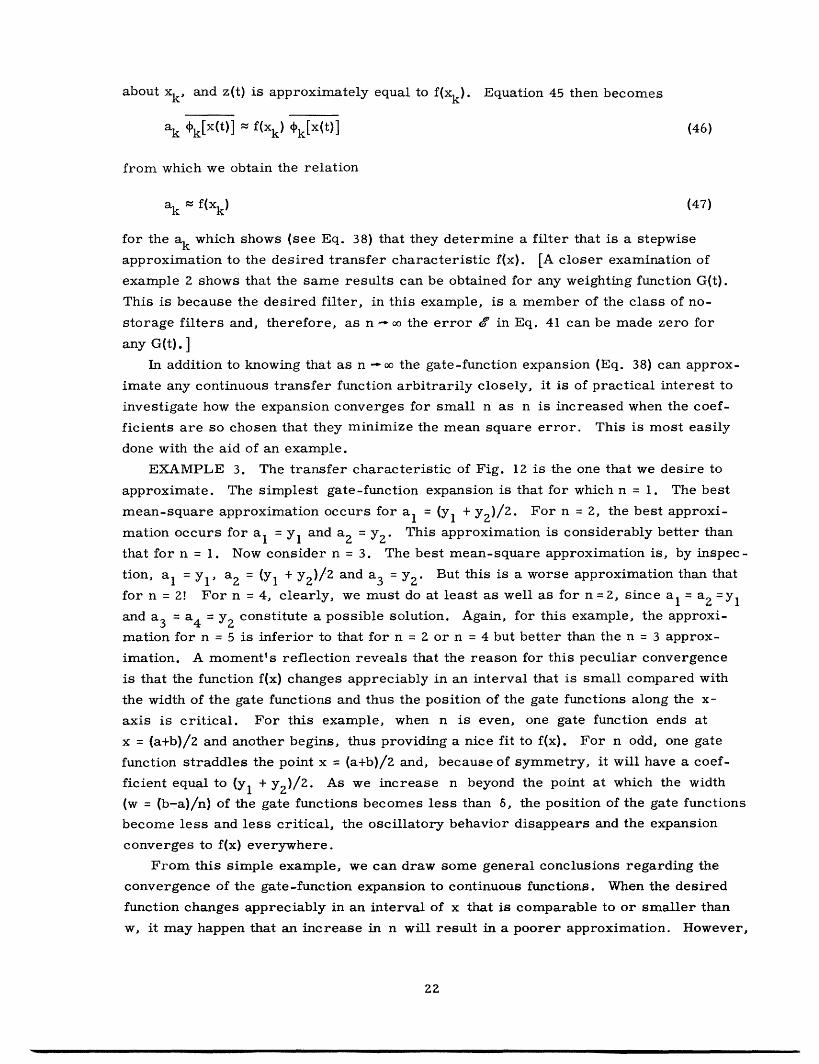
This equation is the desired orthogonal representation for nonlinear systems

involving storage. We now proceed to determine the A for the optimum filter problem.

As in the case of the no-storage filter (Eq. 41), we adopt a weighted mean-square-error

criterion and minimize the error

1=lim zT J G(t) (t)- Aa (a dt (54)

with respect to the coefficients A a. For the coefficient Ap, we have

aa lim 2t - 2G(t) :(P) M- E A (aa dt (55)8A i)

P T-oo

For the error to be a minimum with respect to A D, we set this equation to zero. The

result is

G(t) (p) E Aa (a) = z(t) G(t) ((P) (56)

a

If advantage is taken of the time-domain orthogonality of the i's, this equation reduces

to

Ap G(t) Z2 (p) = z(t) G(t) r(f) (57)

Since the I's are products of gate functions, they can only take on the values zero or

unity; hence Eq. 57 is equivalent to

A G(t) f(D) = z(t) G(t) f(p) (58)

which forms the basis of the experimental procedure for determining the optimum filter

coefficients.

The apparatus for the determination of the optimum filter coefficients is shown in

Fig. 13. An ensemble member of x(t) is fed into the Laguerre network and the cor-

responding ensemble member of z(t) is fed into the product-averaging device. The

outputs of the Laguerre network are fed into a no-memory nonlinear circuit consisting

of level selectors and gate or coincidence circuits. This circuit generates the i's.

Since the I's are either zero or unity, they can be multiplied by G(t) in a simple gate

circuit. The output of this gate circuit is averaged and also multiplied by z(t) and

averaged to yield the two quantities that are necessary to find the optimum coefficients

in accordance with Eq. 58.

26

_t

WEIGHTINGFUNCTION

NETWO (LEVEL SELECTORSG(a)NETWORK CIRCUIT

AVERAGING G(t)()AN G A(t)E CIRCUITS) G M ,)

PRODUCT z~t G(t)0(a)A(t)G(t)0,)rDESIRED FILTER AVERAGING ---OUTPUT z(t)

CIRCUIT

Fig. 13. Experimental procedure for the determination of optimumnonlinear filters involving storage.

xu,~_ _ _--- - OUTPUT

INPUT U2 GENERATOR GAIN At) LAGLUERIRE (LEVEL SELECTORS NETWORK ' ND GTECIRCUITS

Fig. 14. Synthesis of general optimum nonlinear filters in accordance with Eq. 53.

x(t)= FILTER INPUT

V I V t

t)= DESIRED FILTER OUTPUT

I H 1XG(t)= ERROR WEIGHTING TIME FUNCTION

Fig. 15. Example of the use of the error weighting time function.

Fig. 15. Example of the use of the error weighting time function.

27

--�bdba4r

n

�- M ,

Mn2

VV M'A 141o�lh In-. I Arl, 1, Al 1. /,n /--

ZI

IIt

I-

After the optimum coefficients have been determined, the nonlinear system can be

synthesized formally in accordance with Eq. 53, as indicated in Fig. 14. In Fig. 14

we note that the operation from the outputs of the Laguerre network to the system output

y(t) is a no-memory operation. That is, y is an instantaneous function of the Laguerre

coefficients. Once the A's are known, this function is directly specified and any other

method of synthesizing no-storage systems for a prescribed operation can be used.

One such method is described in reference 9.

In the procedure described above for determining and synthesizing optimum nonlinear

filters the use of gate functions in the expansion of Eq. 51 is of central importance. Let

us examine some of the consequences of this:

1. The use of gate functions provides us with a series representation for the output

of the filter in which the time-domain orthogonality of the terms of the series is inde-

pendent of the filter input. This enables us to obtain the optimum filter coefficients

for arbitrary filter inputs without solving simultaneous equations.

2. Since the gate functions are orthogonal with respect to any weighting factor, we

can determine optimum filters for weighted mean-square-error criteria.

3. In most series representations of a function we encounter the difficulty that over

some region of the independent variable small differences of two or more large terms

are necessary to represent the desired function. In the gate-function expansion (Eq. 53)

only one term has a nonzero value at any one instant of time; so this difficulty does not

arise.

4. In general, expansions that represent nonlinear functions involve the use of

multipliers in the experimental circuits. (For example, if a Taylor series or Hermite

function expansion is used.) The use of gate functions replaces the multipliers by

simpler level selectors and coincidence circuits.

3.5 ERROR CRITERION

An error weighting function G(t) appears in the error expressions Eqs. 41 and 54

for the no-storage and the general filter. The choice of this weighting function will,

of course, depend upon the particular problem. It may be chosen as a function of the

past, present, and/or future of x(t) and z(t) and can be generated in the laboratory from

the recorded ensemble members of x(t) and z(t). If G(t) is a constant, then the mean-

square-error criterion results. Other choices for G(t) enable us to design filters for

different error criteria and to introduce a priori information into the filter design. In

this section a few choices of G(t) are discussed. We restrict G(t) to be non-negative,

since the concept of negative error is not meaningful.

One choice of G(t) is illustrated by the following example. Let the signal component'

z(t) of the filter input x(t) consist of amplitude-modulated pulses that occur periodically.

As shown in Fig. 15, x(t) is z(t) corrupted in some way by noise. We assume that we

know when the signal pulses occur. Our object is to determine their amplitude. The

optimum mean-square filter, of a given class of filters, for recovering z(t) from x(t)

28

�

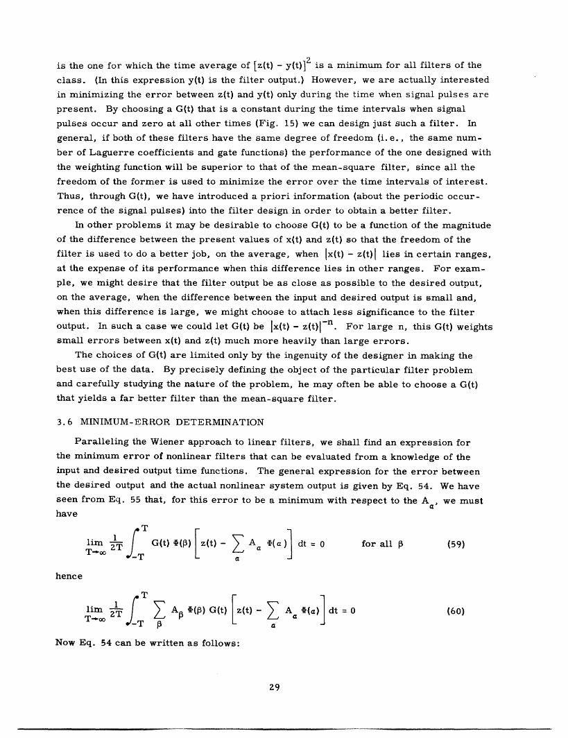
is the one for which the time average of [z(t) - y(t)]2 is a minimum for all filters of the

class. (In this expression y(t) is the filter output.) However, we are actually interested

in minimizing the error between z(t) and y(t) only during the time when signal pulses are

present. By choosing a G(t) that is a constant during the time intervals when signal

pulses occur and zero at all other times (Fig. 15) we can design just such a filter. In

general, if both of these filters have the same degree of freedom (i. e., the same num-

ber of Laguerre coefficients and gate functions) the performance of the one designed with

the weighting function will be superior to that of the mean-square filter, since all the

freedom of the former is used to minimize the error over the time intervals of interest.

Thus, through G(t), we have introduced a priori information (about the periodic occur-

rence of the signal pulses) into the filter design in order to obtain a better filter.

In other problems it may be desirable to choose G(t) to be a function of the magnitude

of the difference between the present values of x(t) and z(t) so that the freedom of the

filter is used to do a better job, on the average, when x(t) - z(t)l lies in certain ranges,

at the expense of its performance when this difference lies in other ranges. For exam-

ple, we might desire that the filter output be as close as possible to the desired output,

on the average, when the difference between the input and desired output is small and,

when this difference is large, we might choose to attach less significance to the filter

output. In such a case we could let G(t) be Ix(t) - z(t)l - n. For large n, this G(t) weights

small errors between x(t) and z(t) much more heavily than large errors.

The choices of G(t) are limited only by the ingenuity of the designer in making the

best use of the data. By precisely defining the object of the particular filter problem

and carefully studying the nature of the problem, he may often be able to choose a G(t)

that yields a far better filter than the mean-square filter.

3.6 MINIMUM-ERROR DETERMINATION

Paralleling the Wiener approach to linear filters, we shall find an expression for

the minimum error of nonlinear filters that can be evaluated from a knowledge of the

input and desired output time functions. The general expression for the error between

the desired output and the actual nonlinear system output is given by Eq. 54. We have

seen from Eq. 55 that, for this error to be a minimum with respect to the A a , we must

have

T

lim T F G(t) (P) z(t)- A (a ) dt = 0 for all B (59)T-oo

hence

T

lim Z AP I(p) G(t) z(t) A ai(a) dt = 0 (60)T-ooZT T a

Now Eq. 54 can be written as follows:

29

- ---- L --- I -- -C --- L---- ---------- "-·-s --

'= G(t) z(t) (t)- A (a)] - Ap (p) G(t) z(t) - a (a3 (61)a Z a

But, from Eq. 60, we see that the term on the right side of Eq. 61 is zero for the

optimum filter. Using this fact and inserting the expression for the optimum filter

coefficients (Eq. 58) in Eq. 61, we obtain the desired expression for the minimum error.

min = (t) G(t) - z(t) G(t) f(a) (62)T e o r G(t) (a)

This equation expresses the error of te optimum system with a given number of

Laguerre coefficients and gate functions in terms of the filter-input and desired output

time functions. If, in Eq. 62, (a) is changed to j(x) and the summation is taken over

j, then we have the minimum-error expression for no-storage filters.

With the addition of a squaring device at the output of the product-averaging circuit

in Fig. 13 the quantities necessary to determine min can be evaluated and Bmin can

thus be found without first constructing the optimum filter. Similar apparatus could

be built to evaluate min automatically upon application of x(t) and z(t). For those

filters that have a sufficiently small number of A (for example, no-storage filters

and simple filters involving one or two Laguerre coefficients) all the terms in the sum

(Eq. 62) could be evaluated simultaneously and added. This would give a rapid way of

finding min' When the number of coefficients becomes very large, then, in order to

save equipment at the expense of time, the terms in the sum could be evaluated sequen-

tially. This apparatus would be useful in deciding a priori the complexity of the non-

linear filter to use for a particular problem. It would also enable us to decide whether

or not it is worth while to construct a complicated nonlinear filter to replace a simple

linear or nonlinear one. Since such apparatus would make use of the same measure-

ments that determine the A , if after measuring its error we decided to build the filter,

we could construct it without further measurements.

3.7 THE STATISTICAL APPROACH

We can shed additional light on the filter theory that was developed in the previous

sections by formulating the same problem on a statistical basis. As before, we shall

characterize the past of the filter input by s Laguerre coefficients u .... , u s and deter-

mine the optimum nonlinear operator that relates these coefficients to the system output

for a weighted mean-square-error criterion.

Consider an ensemble of the Laguerre coefficients ul(t), ... , us(t) and corresponding

ensembles of the system output y(t), the desired output z(t), and the weighting function

G(t). We shall regard ul, ... ,u s , y, z, and G as random variables. We want to find

the y, as a function of the u's, that minimizes the error

30

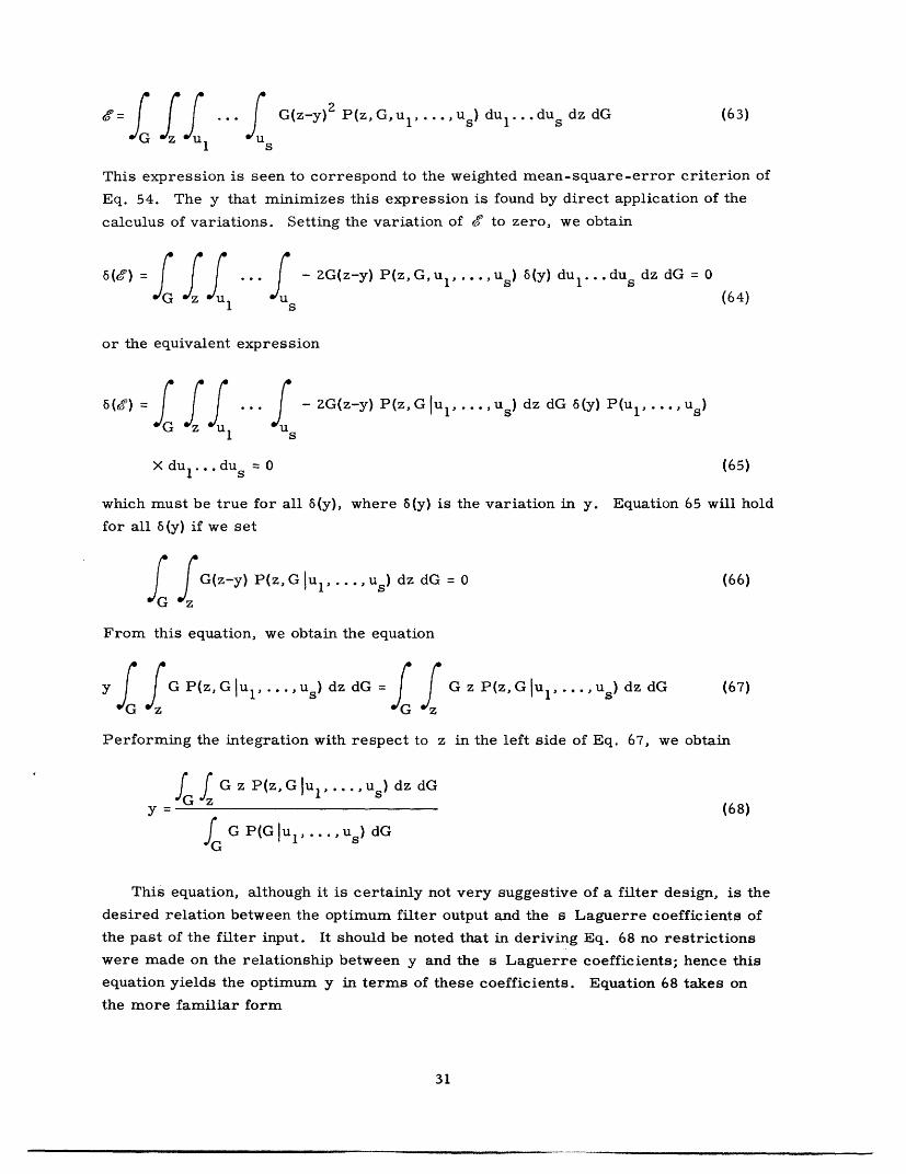
= zu .J ... f G(z-y) 2P(zGul...us) dui...du dz dG (63)1 s

This expression is seen to correspond to the weighted mean-square-error criterion of

Eq. 54. The y that minimizes this expression is found by direct application of the

calculus of variations. Setting the variation of to zero, we obtain

86() =fff * f '-ZG(z-y) P(z,G,ul,... us) (y) du...dus dz dG =

1 Us (64)

or the equivalent expression

6() z = u ,; 4 *-- S -G(z-y) P(z,GIu , ... us) dz dG (y) P(ul, .,.,uS)

s

Xdu1 . . .du s = 0 (65)

which must be true for all 6(y), where 6(y) is the variation in y. Equation 65 will hold

for all 6(y) if we set

f| fzG(z-y) P(z,GIul . U ,s) dz dG = O (66)

From this equation, we obtain the equation

yf fG GP(zGul -u)dz dG =ff; G z P(z G 1,.... u s) dz dG (67)

Performing the integration with respect to z in the left side of Eq. 67, we obtain

I G z P(zGIlul'...Us) dz dG

Y = Z (68)

GG P(G ul ..... us) dG

This equation, although it is certainly not very suggestive of a filter design, is the

desired relation between the optimum filter output and the Laguerre coefficients of

the past of the filter input. It should be noted that in deriving Eq. 68 no restrictions

were made on the relationship between y and the s Laguerre coefficients; hence this

equation yields the optimum y in terms of these coefficients. Equation 68 takes on

the more familiar form

31

_ __ � C_ �� _---11_1 _·---· I _ --- I

= z P(zu 1 ... us )dz (69)

when G is a constant, corresponding to the mean-square-error criterion. In this case

we have the result that the optimum output for a given past of the input is just the con-

ditional mean of the desired output, given this past of the input.

Let us now investigate the relation between the result of the statistical approach

(Eq. 68) and that of the so-called time-domain approach (Eq. 58). We shall express

both of the time averages in Eq. 58 as ensemble averages and then compare the result

with Eq. 68. The average on the left side of Eq. 58 is equal to

G(t) (a) = S .} *.*J G (a) ( ,*..us) P(u I) P(ul ...,us) dG dul...dus

1 2

(70)

For the present, let us assume that the width of the gate functions is so small that the

u's are essentially constant over each cell in the function space. Then Eq. 70 can be

written

G(t) (a) P * ush (,(u I',Au5 ) f GP(GIu 1 . .. ush)dG (71)

thin which the factor multiplying the integral is just the probability that the a cell in

the function space is occupied.

By a similar procedure we obtain for the average on the right side of Eq. 58,

G(t) z(t) (a) P 1 Uh) (ul .Au) i G z PGul, , u dG dz

(72)

Using Eqs. 71 and 72 in Eq. 58, we obtain

fGf (z G Ui .., ush dG dz

(73)

G P(GJul ... ,Ush dG

Recall that A is just the system output when the ath cell in the function space is

occupied. Thus, as the cells become smaller, the system determined by Eq. 58

approaches the optimum system of Eq. 68.

Let us now remove the restriction on the size of the cells. For simplicity in

interpreting the results, we shall let G = 1. For this value of G, the weighted

32

I

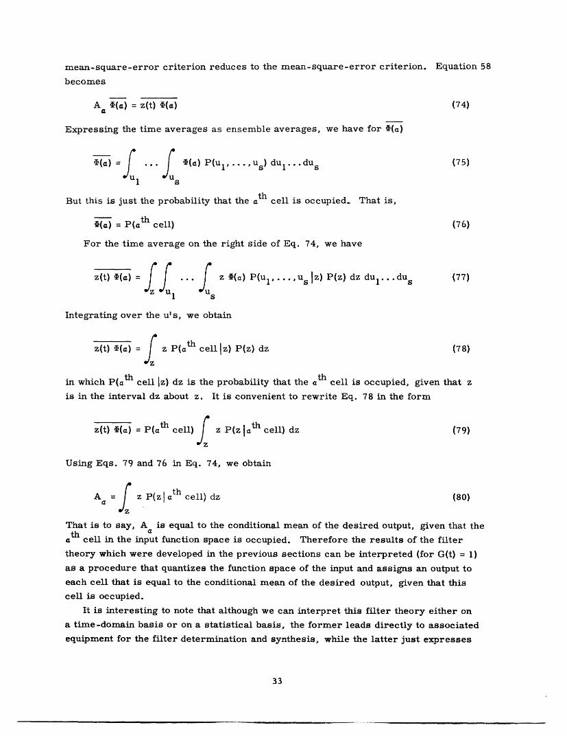
mean-square-error criterion reduces to the mean-square-error criterion. Equation 58

becomes

Aa f(a) = z(t) (a) (74)

Expressing the time averages as ensemble averages, we have for f(a)

~(a) =1 f '(a) P(ul,.,Us) dul...dus (75)

thBut this is just the probability that the at h cell is occupied. That is,f(a) = P(ath cell) (76)

For the time average on the right side of Eq. 74, we have

z(t) (a)=z j u "u z(a) P(ul ... suslz) P(z) dz dul...du , (77

1 s

Integrating over the u's, we obtain

z(t) (a) = f z P(ath celllz) P(z) dz (78)

in which P(ath cell z) dz is the probability that the ath cell is occupied, given that z

is in the interval dz about z. It is convenient to rewrite Eq. 78 in the form

z(t) (a) = P(ath cell) z P(z ath cell) dz (79)

Using Eqs. 79 and 76 in Eq. 74, we obtain

A = z P(z ath cell)dz (80)

That is to say, A is equal to the conditional mean of the desired output, given that theth c n

a cell in the input function space is occupied. Therefore the results of the filter

theory which were developed in the previous sections can be interpreted (for G(t) = 1)

as a procedure that quantizes the function space of the input and assigns an output to

each cell that is equal to the conditional mean of the desired output, given that this

cell is occupied.

It is interesting to note that although we can interpret this filter theory either on

a time-domain basis or on a statistical basis, the former leads directly to associated

equipment for the filter determination and synthesis, while the latter just expresses

33

____ � I^ �I_·_ �_·______ �II�

a mathematical relationship between the quantities involved in the problem. For

example, in the simple case in which G(t) = 1, Eq. 80 might suggest that we evaluate

P(z lath cell) for all cells and for all z and then perform the indicated integration.

However, the time-domain approach shows us directly that the convenient quantities

to measure are those of Eqs. 75 and 79, which look quite formidable from the statis-

tical point of view. Furthermore, when we introduce G(t), the problem appears con-

siderably more complicated from the statistical point of view but, as we have seen

from the time-domain approach, it only involves the addition of a single gate circuit

in the experimental apparatus (Fig. 13).

3.8 OPTIMUM NONLINEAR FILTERS FOR A MAXIMUM PROBABILITY CRITERION

We shall now discuss a method for determining a nonlinear filter whose output is

the most probable value of the desired output, given the past of the input. Such a filter

can be determined with a simple modification of the apparatus (Fig. 13) that was used

to determine optimum filters for a weighted mean-square-error criterion.

As in the case of the weighted mean-square-error criterion, we let the form of the

nonlinear operator be that of Eq. 53. At any instant, the system output is equal to the

coefficient of the term that corresponds to the occupied cell in the function space of the

past of the input. Hence, for the maximum probability criterion, we must choose each

coefficient A to be equal to the most probable value of the desired output, given thatth

the at cell is occupied.

An experimental procedure for determining maximum probability filters is shown

in Fig. 16. The desired output z(t) is fed into a level-selector circuit. If the amplitude

of z(t) is in the amplitude interval corresponding to the level zj, then the output at the

j terminal of the level selector is unity, otherwise it is zero. The outputs of the

level-selector circuit, along with the output of the generator, are fed into gate

circuits. The output of the jth gate circuit is unity when z(t) is in the amplitude interval

GIVEN......o

Fig. 16. Experimental procedure for the determination of optimum filtersfor a maximum probability criterion.

34

about z. and, simultaneously, the ath cell in the function space is occupied. It is zeroJ

at all other times. The time average of this output is the probability of the simultaneous

occurrence of these two events. We shall write this probability as P(zj, ath cell). But

P(zj, ath cell) = P(zj la th cell) P(ath cell) (81)

so that the output of the jth averaging circuit is proportional to P(z j lath cell). If ter-

minal k has the largest output of all the m terminals, then zk is the most probable

value of z(t), given that the ath cell is occupied. [It is, of course, assumed that m

is large enough so that the amplitude interval associated with z is very small compared

with the maximum amplitude of z(t)]. Hence the optimum Aa for the maximum proba-

bility criterion is equal to zk.

For convenience in rapidly determining which output of the averaging circuits is

largest, the outputs can be displayed on an oscilloscope as indicated in Fig. 16. Once

the A's are determined, the filter can be synthesized in the standard form shown in

Fig. 14.

3.9 IMPROVING THE PERFORMANCE OF A GIVEN FILTER

As we increase the complexity of the filter (i.e., we use more Laguerre coefficients

to characterize the past and more gate functions for each coefficient) the number of A

that are necessary to specify the filter grows very rapidly. In particular, if we use s

Laguerre coefficients and n gate functions for each coefficient, we have n s A to eval-a

uate. After evaluating a large number of A , we should like to have some guarantee that

our filter would perform at least as well as, say, a linear filter or a simple nonlinear

filter that can be designed with less effort. Methods of obtaining this guarantee will now

be described.

Let us, first of all, prove the existence of a property of our class of filters which

will be used in one of the methods. We want to show that the class of filters employing

s Laguerre coefficients includes the class of filters that only uses any one of the s

Laguerre coefficients. Since we can always renumber the Laguerre coefficients, it is

sufficient to prove that the s-coefficient class includes the class that uses only the first

Laguerre coefficient u1 . The series representation for the general system of this one

coefficient class is

n

y(t) = ai 4i(Ul ) (82)i=l

We now make use of the fact that the sum of the n gate functions of any one coefficient

is unity, in order to express the series representation (Eq. 82) in the form

35

-- I - -- .__ __ __ -------I - -

Uo

GIVENFILTERINPUT x (t)

Aa G(t)d (a)

DESIREDFILTEROUTPUT

WEIGHTINGFUNCTION

G (t)

_

G (t) 0 (a)

z (t)

Fig. 17. Augmenting the Laguerre coefficients with the outputof a given filter F to determine a filter with a betterperformance than that of F.

r---------------------

INPUT FILTER OUTPUTF - NO-STORAGE

FILTER

L…J~~~~~~~~~~~~~~~~~~~~~~~~~~~~

Fig. 18. The class of filters that consists ofcascaded with a no-storage filter.

a given filter F

Fig. 19. Synthesis of the filter with coefficients determinedin accordance with Fig. 17.

36

) S>(a)

z (t)G(t) (a)

z (t) G (t) (a)

y(t) = ai i(ui) j( 2) +k(U3) * * *h(Us ) (83)i=l j=l k=l h=l

which is recognized to be a special case of the expansion (Eq. 51) for the general

s-coefficient system. In a similar way, it can be shown that the class of filters using

s Laguerre coefficients includes all classes having less than s coefficients. Note that

this property is independent of the nature of the u's; they may be Laguerre coefficients

of the past of x(t) or they may be obtained from x(t) by any linear or nonlinear operation.

We now make use of this property to determine a filter whose performance is equal

or superior, with respect to a weighted mean-square-error criterion, to a given filter

F. F may be linear or nonlinear. We augment the Laguerre coefficients with the out-

put, u, of the given filter F, as shown in Fig. 17. Then, by the property demonstrated

above, the filter whose output is expressible as

n

y(t) = ai i(Uo) (84)i=l

is a member of the class of filters which has s Laguerre coefficients augmented by u0 .

If the number n of gate functions associated with the variable u is sufficiently large,

then, to any degree of approximation, Eq. 84 represents the class of filters shown in

Fig. 18 - the class which consists of F cascaded with a no-storage filter. Since the

transfer characteristic of the no-storage system can be linear, the class of filters

shown in Fig. 18 certainly contains the filter F. Hence the filter that is determined

by the procedure indicated in Fig. 17, for any s, performs at least as well as the given

filter F and, in fact, at least as well as F cascaded with any no-storage filter.

After the A of the desired filter have been determined, as indicated in Fig. 17,

the filter synthesis is accomplished as shown in Fig. 19.

We now turn to another method of determining filters to improve the performance

of given filters. Let the output of the given filter F be uo(t) when its input is x(t).

Our object is to improve (with respect to a weighted mean-square-error criterion) the

performance of F by paralleling it with a filter which will be determined. The A ofa

the desired filter are those that minimize the error

T

:= limr T 1 G(t) (t) - [o(t) + A i(a dt (85)T-oT a

a

This expression is seen to be equivalent to

lim ~ G~T 2

: lir - G(t) z(t)- Uo(t)]- EA *(a) dt (86)

a e

37

_ �� __ ___ s_ 1�_1 __I___I� �I_� ·1

WEIGHTINGFUNCTION

G(t)

Aa G(t){a)l = [z(t)-u,(t)] G(t)0(a)

Fig. 20. Apparatus for the determination of a filter to improve the performanceof F by a parallel connection.

Comparing Eq. 86 with Eq. 54, we see that the optimum A are determined by an

experimental procedure like that indicated in Fig. 13, with z(t) replaced by z(t) - uo(t).

The latter quantity is easily obtained by applying x(t) to the given filter F and subtracting

the output of F from z(t), as shown in Fig. 20. The parallel combination of F and the

filter, determined as we have just described, will always perform at least as well as

F, since that filter which has no transmission from input to output is a member of the

class of filters considered in our theory. In other words, the solution in which all the

A are equal to zero is a possible solution of Eqs. 84 and 85.

The second method described for improving the performance of given filters offers

the advantage of not having gate functions associated with the output time function of the

given filter; therefore, improvements can be made on the performance of F by very

simple systems that involve as few as one Laguerre coefficient and thus have a rela-

tively small number of A to evaluate. The first method does require a gate-function

expansion of the output of the given filter F but it has the advantage of ensuring that

the performance of the resultant filter will always be at least as good as the performance

of F cascaded with any no-storage system. In either method, the resultant over-all

filter approaches the most general filter (of the class considered in this theory) as the

number of Laguerre coefficients and gate functions is increased.

Still another design procedure involves the determination of that filter which, when

cascaded with F (with F as the first member of the combination), yields an over-all

filter with a performance superior to that of F alone. In order to ensure that the

resultant over-all filter performs at least as well as F, we could augment the Laguerre

coefficients of the cascaded filter by a variable u that is equal to the input of the

Laguerre network. While this procedure gives a filter that is at least as good as F,

we have no assurance that as the number of Laguerre coefficients and Hermite functions

is increased the over-all filter will approach the most general filter.

38

s

3.10 MULTIPLE NONLINEAR PREDICTION

The problem of multiple prediction is that of predicting a time series from a knowl-

edge of related time series. An example, cited by Wiener, is the prediction of weather

at one location from a knowledge of the past of the weather at that and other surrounding

locations.

The filter theory developed in the preceding sections is easily extended to the

problem of multiple prediction. Let z(t+a) be the function that we desire to predict and

let xl(t) through xp(t) be the input functions on whose past we operate to form our pre-

diction. The set of functions xl(t) through xp(t) may, indeed, include z(t). We shall

characterize the past of each input by a set of Laguerre coefficients. Let jul ju 2 . . ju s

be the Laguerre coefficients of xj(t). Now let us think of a function space that encom-

passes the past of all p of the input time functions. That is, the basis of this space

is formed by the Laguerre functions associated with each input. A point in this space

then represents the past of all the inputs and thus the multiple prediction problem is

just the problem of mapping this space onto a line (corresponding to the amplitude of the

system output) in a manner that is optimum with respect to some error criterion. But

this is the same problem encountered in the single-input filter problem and we recog-

nize that the only difference between the single- and multiple-input problems is in the

number of dimensions of the function space. The solution of the multiple prediction

problem directly parallels that of the filter problem given in section 3.4.

We let y(t) be a gate-function expansion of the Laguerre coefficients of all the inputs

x 1(t).. . xp(t). The expansion is

il jl h I jp hp p

X ~il(lUl) fj(lUZ) . * * * s.) p(p2U) '" *h (pUs) (87)1 d (I u1 ) dji(Iu2 ) 1 (p h (87)

If we associate an Q(a) with each product of 's in Eq. 87 and let Aa be the corresponding

coefficient a ... h Eq. 87 takes the simplified forml' 'h 1 ... .. ip' p p

y(t) = A. Q(a) (88)a

Just as in the filter problem (sec. 3.4), we adopt a weighted mean-square-error

criterion and minimize the error

of= lim zf G(t) z(t+a)- A (a dt (89)T.~o O ,/_/ (z z ,}a

39

_______IIIY·_I1ICI___ICll__llll___q___l_ �. ..__. _ � 111 1 -I-

-G(t)

) (a)

a) G(t)a (a)

Fig. 21. Experimental procedure for the determinationof the optimum multiple predictor.

y (t)

Fig. 22. Synthesis of the optimum multiple predictor.

TRANSFER NO-STORAGE -NONLINEAR

(t)

Fig. 23. The class of nonlinear systems that has no cross productsof the Laguerre coefficients.

40

INPUT

INPUT

This equation is seen to have the same form as Eq. 54 for the filter problem. The

solution for the optimum A proceeds exactly as in section 3. 4, with the result that

A G(t) Q(a) = z(t+a) G(t) Q(a) (90)

The apparatus for experimentally determining the A according to this equation is

shown in Fig. 21. After the coefficients have been determined, the predictor can be

synthesized in accordance with Eq. 88, as shown in Fig. 22.

IV. LINEAR AND SIMPLE NONLINEAR SYSTEMS

4.1 A TEST FOR THE COEFFICIENTS

Once the coefficients for an optimum filter have been determined, the filter can,

as we have seen, be synthesized formally, as shown in Fig. 14. From the standpoint

of apparatus, much simpler synthesis procedures exist, however, if the filter is linear

or belongs to a particular subclass of nonlinear systems. Hence it is desirable to have

a means of detecting linear and simple nonlinear systems directly from a knowledge of

their characterizing coefficients. We shall develop a simple procedure for testing the

coefficients (A ) that detects such systems and directly yields a convenient synthesis

of them.

The class of simple nonlinear systems that we shall consider is shown in Fig. 23.

It consists of a Laguerre network and no-storage nonlinear two-pole circuits (no-storage

nonlinear systems with one input and one output terminal). Each output of the Laguerre

network is fed into one no-storage two-pole circuit and the outputs of these circuits are

added to form the system output y(t). In this class of systems the nonlinear circuits

introduce no cross talk among the Laguerre coefficients (i. e., no cross products of

Laguerre coefficients are introduced). This class of systems is clearly a subclass of

the general class considered in Section III. When the transfer characteristics of all the

two-pole circuits are straight lines, the system is linear. In particular, it is an sth-

order Laguerre network in which the gain factors associated with the Laguerre network

outputs are equal to the slopes of the respective linear two-pole transfer characteristics.

The synthesis of nonlinear systems belonging to this subclass is relatively simple.

The nonlinear two-pole circuits can be synthesized by piecewise-linear approximations

with the use of diodes and resistors. If the system is linear, the synthesis takes the

form of a Laguerre network whose outputs are properly amplified or attenuated before

being added to form the system output. In this linear case it may be desirable to

measure the transfer function of the optimum system and then use available synthesis

techniques to obtain alternate realizations of this transfer function by using linear

passive circuits.

We now investigate the determination, from the characterizing coefficients A , of

a nonlinear system, if the system belongs to the class shown in Fig. 23. If it does, we

41

_ ���__l_--Y····�·ll--111·1 ·IIII�--·IIU-UYI·LIC--II-�- ~ ~ ~ ~ ~ ~ ~

shall investigate the determination of the transfer characteristics of the nonlinear

two-pole circuits.

From the point of view of function space, the subclass of nonlinear systems shown

in Fig. 23 consists of all those systems for which the system output corresponding to

each cell in function space is equal to the sum of the outputs corresponding to the

coordinates (the Laguerre coefficients) of the cell. That is, since there is no cross

talk, each coordinate contributes to the output an amount that is independent of the other

coordinates and thus the system output corresponding to any cell is the sum of the out-

puts corresponding to the coordinates of the cell. (We speak here of cells rather than

points in function space because we represent our nonlinear system by a gate-function

expansion that quantizes the function space. In this connection we should also realize

that we obtain a stepwise approximation to the two-pole characteristics of Fig. 23

rather than the continuous curves.) Hence Eq. 51, which represents a general gate-

function expansion of the Laguerre coefficients, takes on the form

n n n

y(t) = bil i(ul) + Z b 2 j(U 2 ) +... + Z bhs ?h(Us) (91)i=l j=l h=l

for the subclass of systems of Fig. 23. Each sum in the equation yields the transfer

characteristic of the nonlinear two-pole circuit that is associated with the Laguerre

coefficient indicated in that sum. Compare this expansion with that of Eq. 51.

In the experimental procedure described in Section III for finding optimum filters

(Fig. 13) we determine the A or equivalently the ai h.. of the filter. If and only

if these a's are such that Eq. 51 can be expressed in the form of Eq. 91, the system

can be synthesized in accordance with Eq. 91 in the form shown in Fig. 23. Let us

see how the a's must be related to the b's if these two equations are to be equivalent.

By "equivalent" we mean that the two equations yield the same value for every cell in

function space; hence we must have

ai,j, . . ., =bil + bj2 + . +bhs for all i,j, ... ,h (92)

This relation represents a set of ns simultaneous equations which the a's must satisfy.

We shall now develop a simple way of finding out whether or not, for any given set of

a's, this set of equations is satisfied.

It is convenient to establish an order for the evaluation of the a's (and thus the A ).

It is assumed, henceforth, that these coefficients are evaluated as follows. The first

coefficient we evaluate is that for which i = j = ... = h = 1. The next n - 1 coefficients

are obtained by letting h run from 2 to n while all other indices are held equal to

unity. To obtain the (n+l)th coefficient, we set the index preceding h to 2 and let all

other indices be unity. The following n - 1 coefficients are obtained by again letting h

range from 2 to n. We continue this procedure until the index i has gone through all

its n-values, at which point all the a's will have been evaluated. This order of evaluating

42

the coefficients is best illustrated by a simple example.

EXAMPLE 4. Consider the coefficients (a's) of a nonlinear system that has threeLaguerre coefficients and two gate functions for each coefficient. That is, s = 3 and

n = 2. There are n = 8 coefficients a j k to evaluate. According to the above pro-

cedure, these coefficients are evaluated in the following order:

1. all

Z. a 112

3. a12

4. a21ZZ

5. a2 1 1

6. a 2 1 2

7. a 2 2 1

8. a 2 2 2

A study of the order in this simple example is sufficient to establish the order of

evaluating the a's for any s and n.

Now think of the coefficients ai, j ... ,h' arranged in the order of eval-uation, as components of a vector A, and the corresponding coefficients

bllb 21 b b 22 b. b .... bls b2s... bns, arranged as shown, as com-ponents of a vector B. Then the set of equations represented by Eq. 92 can be written

in matrix form as follows:

A] = [M] B] (93)

where [M] is the matrix that operates on the vector B to give the vector A. Let us

determine the form of the matrix [M]. In order to illustrate the form of this matrixwe shall consider a nonlinear system for which s = n = 3 and for which Eq. 92 is

assumed to hold. From the results of example 4 the form of [M] can be visualized

for any s and n. The equations indicated in Eq. 92 are given, for this example, in

Table I. The b's are written at the top of the columns so that the form of the matrix

[M] is evident. The actual equations are obtained by dropping the b's down beside theunity coefficients. (All the blank spaces in the matrix represent zero matrix coeffi-

cients.) Thus the first equation reads

al 1 = bl 1 + b1 2 + b13 (94)

We see that the matrix [M] is composed entirely of zeros and ones. We also note theregular pattern of the unity coefficients. A study of this pattern will enable the readerto visualize its form for any s and n.

We now state a test for the a's that enables us to determine directly whether or notthe set of equations (Eq. 92) or, equivalently, Eq. 93 is satisfied. The test wasdeveloped from a study of [M] and its validity can be checked (for s = n = 3) by analyzingit in terms of the matrix of Table I.

1. Starting with al, 1, . 1' plot the a's (consecutively in the order in which theyare evaluated) in groups of n at unit intervals along a linear scale. That is, form aset of n(s - l ) graphs, each of which contains n a's plotted at equal intervals along a

43

_______IIII__YILIIIslpl_ ·I��··--·IIII�-_II-___�_·-_ 1_1 ---_

alll

a1 1 2

a1 1 3

aIzIa1 2 1

a1 2 2

a1 2 3

a1 31

a1 32

a1 3 3

a2 1 1

a2z1 2

az1 3

aZZ1

a2 2 2

a2 2 3

a2 3 1

a2 32

a2 3 3

a3 1 1

a3 1 2

a3 1 3

a3 2 1

a3 2 2

a3 2 3

a3 3 1

a3 3 2

a3 3 3

bll

= 1

= 1

= 1

= 1

= 1

= 1

= 1

= I

Table I

b2 1 b3 1 b1 2 b2z b3 2 b1 3 b2 3 b3 3

1 1

1 1

1 1

1 1

1

1

1 1

1

1

1

1

1

1

1

1

1

1

1 I

1

1

1

1

1

line. Call this set of graphs set 1.

2. Take the first "a" of each graph above, starting with al,1 1' and plot these

consecutively in groups of n at unit intervals on a linear scale. Call this set of graphs

set 2.th

3. Repeat the procedure of step 2 until s sets of graphs are obtained. The s set

will consist of only one graph.

From a study of the general form of [M] it can be seen that if, for a given set of a's,

there exists a set of b's that are such that Eq. 93 is satisfied, then all of the graphs of

these a's within each set of graphs will be identical, except for a possible vertical trans-

lation. Furthermore, the converse holds; that is, if all of the graphs of the a's within

44

1

1

1

1

1

each set of graphs are identical, within a vertical translation, then there exists a set

of b's that are such that Eq. 93 is satisfied.

Hence, if there exists a system governed by Eq. 91 that is equivalent to a system

governed by Eq. 51 for a given set of a's, then all the graphs of the a's within each set

of graphs must be the same, except for a possible vertical translation. And, con-

versely, if we apply the above test to the a's of a system and find that all the graphs

within each set are the same, within vertical translation, we know that the system

that has these a's can be synthesized in the form shown in Fig. 23.

4.2 SYNTHESIS PROCEDURE

In this section we assume that the a's have been tested as described above and that

they correspond to a system of the type shown in Fig. 23. We are now concerned with

the synthesis of this system. In particular, we want to find the transfer characteristics

of the no-storage two-pole circuits. One way to do this is to solve Eq. 93 for the b's,

which, by Eq. 91, directly determine the no-storage transfer characteristics. As a

consequence of the special form of [M], this solution is readily accomplished. However,

a simpler method of synthesizing the desired system makes direct use of the graphs that

are drawn when the a's are tested. Referring to the previous section, let us examine,

relative to the a's in Table I, the sets of graphs defined in the test procedure. From

inspection of Table I it is readily seen that all the graphs of set 1 are identical to

(except for a possible vertical translation) the graph that would be obtained if bl 3 , b 2 3,

and b33 were plotted, in this order, at unit intervals on the same linear scale. Simi-

larly, it is seen that the graphs of set 2 are the same (within a vertical translation) as

the graph that would be obtained by plotting b 1 2 , b22, and b3 2. And, finally, the graphs

of set 3 correspond, in a similar manner, to the graph that would be obtained by plotting

bll, b21, and b31. But notice (Eq. 91 for n = s = 3) that bl3, b23, and b33 are just the

heights of the steps in the stepwise approximation to the two-pole characteristic asso-

ciated with u 3 . Similarly, b 1 2 , b 2 2 , and b3 2 determine the transfer characteristic of

the nonlinear two-pole circuit whose input is u2 . And, finally, bl, b2 1 , and b3 1 deter-

mine the two-pole characteristic associated with ul. Hence the graphs that are made

when the a's are tested directly determine the desired two-pole transfer characteristics,

within a vertical translation. In the synthesized nonlinear system (Fig. 23) the vertical

displacement of the two-pole transfer characteristics affects only the dc level of the

output. When this level is of interest it can be re-established by a series battery at

the system output, as will be shown in examples that follow.

Now we can readily generalize to the case of arbitrary s and n. Except for a

vertical translation, the graph of set 1 determines the transfer characteristic of the

two-pole circuit associated with u s . The graph of set 2 determines the transfer charac-

teristic of the two-pole circuit associated with Us 1' and so on, down to the graph of

set s, which determines the transfer characteristic of the two-pole circuit associated

with u 1.

45

_I_ IC___IIYYIII�_II___·1_LI-(-·IIIII--C . ��.�.�.�.---I----� ___ __-·---- -- -

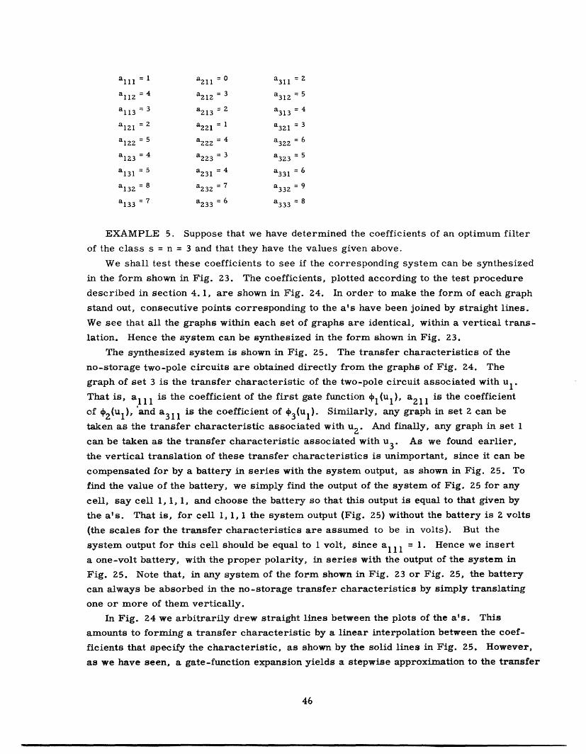
al a21 1 21 1 a3 1 1 2

a1 12 =4 a2 1 2 =3 a3 1 2 = 5

aa21 1 3 3 a2 13 313 4

a1 2 1 =2 a2 2 1 1 a32 1 =3

a1 2 2 = 4 3 2 2 =6

a1 2 3 4 a2 2 3 323=

a1 3 1 5 a231 4 a331 6

a3 8 a =7 a = 913 2 2 3 2 332

a1 3 3 27 a33 6 a333 = 8

EXAMPLE 5. Suppose that we have determined the coefficients of an optimum filter

of the class s = n = 3 and that they have the values given above.

We shall test these coefficients to see if the corresponding system can be synthesized

in the form shown in Fig. 23. The coefficients, plotted according to the test procedure

described in section 4.1, are shown in Fig. 24. In order to make the form of each graph

stand out, consecutive points corresponding to the a's have been joined by straight lines.

We see that all the graphs within each set of graphs are identical, within a vertical trans-

lation. Hence the system can be synthesized in the form shown in Fig. 23.

The synthesized system is shown in Fig. 25. The transfer characteristics of the

no-storage two-pole circuits are obtained directly from the graphs of Fig. 24. The

graph of set 3 is the transfer characteristic of the two-pole circuit associated with ul.

That is, all is the coefficient of the first gate function l1 (ul), a211 is the coefficient

of 2 (ul), 'and a311 is the coefficient of + 3 (U1 ). Similarly, any graph in set 2 can be

taken as the transfer characteristic associated with u Z . And finally, any graph in set 1

can be taken as the transfer characteristic associated with u3. As we found earlier,

the vertical translation of these transfer characteristics is unimportant, since it can be

compensated for by a battery in series with the system output, as shown in Fig. 25. To

find the value of the battery, we simply find the output of the system of Fig. 25 for any

cell, say cell 1, 1, 1, and choose the battery so that this output is equal to that given by

the a's. That is, for cell 1, 1, 1 the system output (Fig. 25) without the battery is 2 volts

(the scales for the transfer characteristics are assumed to be in volts). But the

system output for this cell should be equal to 1 volt, since a111 = 1. Hence we insert

a one-volt battery, with the proper polarity, in series with the output of the system in

Fig. 25. Note that, in any system of the form shown in Fig. 23 or Fig. 25, the battery

can always be absorbed in the no-storage transfer characteristics by simply translating

one or more of them vertically.

In Fig. 24 we arbitrarily drew straight lines between the plots of the a's. This

amounts to forming a transfer characteristic by a linear interpolation between the coef-

ficients that specify the characteristic, as shown by the solid lines in Fig. 25. However,

as we have seen, a gate-function expansion yields a stepwise approximation to the transfer

46

_·

Fig. 24. Graphs of the coefficients in Example 5.

Fig. 25. The nonlinear filter of Example 5.

47

� __ 1_�__1�___� -1_-11111�--·--··-·1�··11111 ·-111_1 1

I0

--

CWU)

"I

I'-w5 i

0 at 311 u

Fig. 26. Graphs of the coefficients in Example 6.

Fig. 27. The filter of Example 6.

48

_j

·I_·_I~JLJK I ~i . a,. *

I

5

I

3

il

I'

U)

-

characteristic in which the height of each step is equal to the corresponding coefficient

in the expansion. This step curve is shown by dotted lines in Fig. 25.

EXAMPLE 6. Again, we consider a filter of the class s = n = 3. Let the coefficients

for this filter be

all a211 = 211 a311 =-1

all =2 a 2 1 2 = 1 a312 0

all3 3 a213 2 a313 = 1

ain 3 a221 2 a321 1121 =3 221 =2 321 =1

a122 4 a222 3 a32 =2

a123 5 a223 4 a323 3

a31 5 a231 =4 a331 =3

a132 6 a232 5 a332 4

a133 =7 a233 =6 a333 =5

These coefficients, plotted according to the test procedure described in section 4. 1,

are shown in Fig. 26. We see that all the graphs within each set of graphs are identical,

within a vertical translation, and, furthermore, we see that they are all linear. Hence

the system can be synthesized as shown in Fig. 27. The transfer characteristics of the

no-storage two-poles are found directly from the graphs of Fig. 26, as discussed in

example 5. The solid lines in the transfer characteristics of Fig. 27 indicate a linear

interpolation between the coefficients that specify these characteristics. Since these

solid-line transfer characteristics are all linear, they can be replaced by amplifiers

whose gains are equal to the slope of the lines.

4.3 APPROXIMATING FILTERS BY LINEAR AND SIMPLE NONLINEAR FILTERS

We have seen that, if the graphs of the characterizing coefficients (the a's) of a

system satisfy certain conditions, the system can be synthesized in the relatively

simple form shown in Fig. 23 and that under certain additional conditions the system

is linear and the synthesis even simpler. In practical problems it is unlikely that the

system coefficients will exactly satisfy these conditions. However, the relative sim-

plicity of the systems of Fig. 23 makes it worth while for us to determine when a more

complicated system can be approximated by one that has this simple form.

The concept of approximating one system by another is meaningful only when we

specify a criterion for the approximation and specify the degree of approximation

relative to this criterion. In this section we consider the approximation of one system

by another from the point of view of two different error criteria.

We first consider the weighted mean-square-error criterion defined by Eq. 54.

Relative to this criterion, we ask how much error is introduced if we change the

49

� __ _�_ __ __�_ _�·�

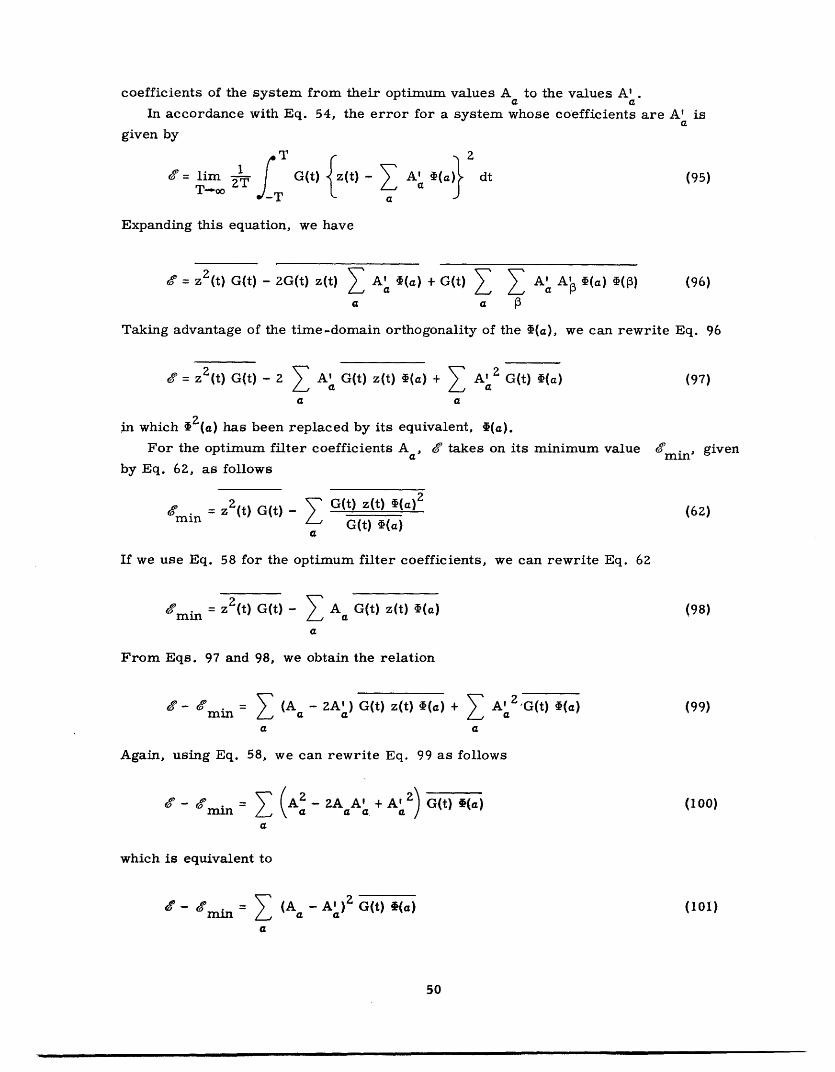
coefficients of the system from their optimum values A to the values A' .a a

In accordance with Eq. 54, the error for a system whose coefficients are A' isa

given by

T- rT f G(t) (t)- A' * (a) dt (95)=lir 2ZT fa (95z(t)T--oo

a

Expanding this equation, we have

g = z 2 (t) G(t) - 2G(t) z(t) Aa' (a) + G(t) A A (a) (P) (96)

a a 13

Taking advantage of the time-domain orthogonality of the (a), we can rewrite Eq. 96

g= z (t) G(t) - 2 A' G(t) z(t) f(a) + Z A' 2 G(t) (a) (97)

a a

in which 2 (a) has been replaced by its equivalent, i(a).

For the optimum filter coefficients A g takes on its minimum value 'min' given

by Eq. 62, as follows

rnin = z 2 (t ) G(t) G(t) z(t) (a)2G(t) (a)a

If we use Eq. 58 for the optimum filter coefficients, we can rewrite Eq. 62

gmin = z 2 (t) G(t) - z Aa G(t) z(t) () (98)a

From Eqs. 97 and 98, we obtain the relation

'- min = (A - 2Aa) G(t) z(t) (a) + 3 A' 2 'G(t) (a) (99)a a

Again, using Eq. 58, we can rewrite Eq. 99 as follows

- min = Z (A - 2A A' + A2) G(t) f(a) (100)a

which is equivalent to

- min = (A -A')Z G(t) i(a) (101)a

50

I

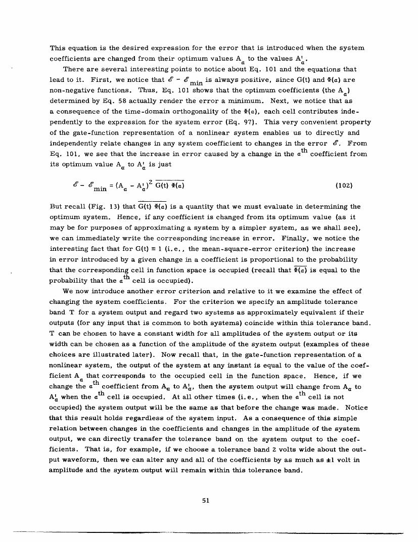
This equation is the desired expression for the error that is introduced when the system

coefficients are changed from their optimum values A to the values A'a aThere are several interesting points to notice about Eq. 101 and the equations that

lead to it. First, we notice that - min is always positive, since G(t) and (a) are

non-negative functions. Thus, Eq. 101 shows that the optimum coefficients (the Aa)

determined by Eq. 58 actually render the error a minimum. Next, we notice that as

a consequence of the time-domain orthogonality of the f(a), each cell contributes inde-

pendently to the expression for the system error (Eq. 97). This very convenient property

of the gate-function representation of a nonlinear system enables us to directly and

independently relate changes in any system coefficient to changes in the error . From

Eq. 101, we see that the increase in error caused by a change in the at h coefficient from

its optimum value Aa to A' is justa a

"- 6 min = (Aa - A )2 G(t) (a) (102)

But recall (Fig. 13) that G(t) (a) is a quantity that we must evaluate in determining the

optimum system. Hence, if any coefficient is changed from its optimum value (as it

may be for purposes of approximating a system by a simpler system, as we shall see),

we can immediately write the corresponding increase in error. Finally, we notice the

interesting fact that for G(t) 1 (i.e., the mean-square-error criterion) the increase

in error introduced by a given change in a coefficient is proportional to the probability

that the corresponding cell in function space is occupied (recall that (a) is equal to the

probability that the ath cell is occupied).

We now introduce another error criterion and relative to it we examine the effect of

changing the system coefficients. For the criterion we specify an amplitude tolerance

band T for a system output and regard two systems as approximately equivalent if their

outputs (for any input that is common to both systems) coincide within this tolerance band.

T can be chosen to have a constant width for all amplitudes of the system output or its

width can be chosen as a function of the amplitude of the system output (examples of these

choices are illustrated later). Now recall that, in the gate-function representation of a

nonlinear system, the output of the system at any instant is equal to the value of the coef-

ficient A that corresponds to the occupied cell in the function space. Hence, if wea th

change the a coefficient from A to Aa, then the system output will change from Aa to

Aa when the at h cell is occupied. At all other times (i. e., when the at h cell is notoccupied) the system output will be the same as that before the change was made. Notice

that this result holds regardless of the system input. As a consequence of this simple

relation between changes in the coefficients and changes in the amplitude of the system

output, we can directly transfer the tolerance band on the system output to the coef-

ficients. That is, for example, if we choose a tolerance band 2 volts wide about the out-

put waveform, then we can alter any and all of the coefficients by as much as 1 volt in

amplitude and the system output will remain within this tolerance band.

51

�--_1___-···11111�··-··I�- 1 --- - I�---L-l�.. -I�--^I

In the optimum filter problem (for the case G(t) - 1) if we alter any coefficient from

its optimum value Aa to Aa, in addition to knowing that the system output will change

from Aa to Aa when the ath cell is occupied, we know the probability of the occur-

rence of this error. This probability is just (a) which was measured in the process

of determining Aa.

In summary, when any filter coefficient is changed from its optimum value Aa to

Al, we can immediately determine the following quantities:

1. The change in the weighted mean square error.

2. The tolerance band relating the optimum and the altered systems.

3. For the case G(t) 1, the probability that the output of the altered system will

differ from that of the original optimum system.

Conversely, if we specify upper limits on any of these quantities, we can find the

permissible variation in the A a. In this respect, it is most convenient to specify a

tolerance band, for, as we have seen, the same tolerance band can be applied to the

system coefficients, thus directly determining their maximum permissible variation.

Furthermore, of the three quantities listed above, the tolerance band is the only one

whose specification determines the permissible range of the A a independently of the

system input. Hence, this criterion is truly characteristic of the system itself. (More

precisely, it is characteristic of the gate-function representation of the system.)

Henceforth, when we speak of two systems as being nearly equivalent it is understood

that this "equivalence" holds with respect to some suitably chosen tolerance band. To

illustrate these concepts we consider an example of a nearly linear system.

EXAMPLE 7. Let the coefficients of an optimum mean-square filter be the same

as those of example 6 with the one difference that a22 = 3. 5 instead of 3. 0. The graphs

of these coefficients are shown in Fig. 28. It is recognized that these graphs do not

satisfy the conditions (sec. 4. 1) for synthesis in the simple form of Fig. 23. However,

let us establish a tolerance band of ±0. 5 volt about the system output and ask if there

is a linear system that is nearly equivalent to this system. In Fig. 28 the dashed lines

in each graph indicate the 0. 5-volt tolerance band. Inspection of this figure shows

immediately that the system is nearly linear with respect to this tolerance band. All

the graphs are linear except one (shown circled) and this one can be made linear, with

the same slope as the other graphs of set 1, without exceeding the tolerance band, as

shown by the dotted line. Hence this system is nearly equivalent to that of example 6

and can thus be approximated by the simple linear system of Fig. 27. Furthermore,

by Eq. 102, the increase in the mean square error, when this optimum system is

approximated by the linear system, is

g - min =(3.5- 3.0)2 (2,2,2) (103)

where (2, 2, 2) is one of the measurements that was made in determining a 2 2 2 . Finally,

we see that the output of the linear system of Fig. 27 will differ from that of the optimum

52

0 1 2 3 UNI

313

- 0 131

a

/Il~

0

/0231

a 221///

a

a //'

0211/,,/'-

Fig. 28. Graphs of the coefficients of a nearly linear system.

VOLTS

IANCE

0321

3 UNITS2

Fig. 29. Example of a 10 per cent tolerance band on a graph of system coefficients.

53

II_ _I_ � _ I _I _ �1_1 _�I_� _^___ �I��I��� -^-----I·X--·IIIIUI II -·II_ �- - - - -

.-

was

I -.iZ

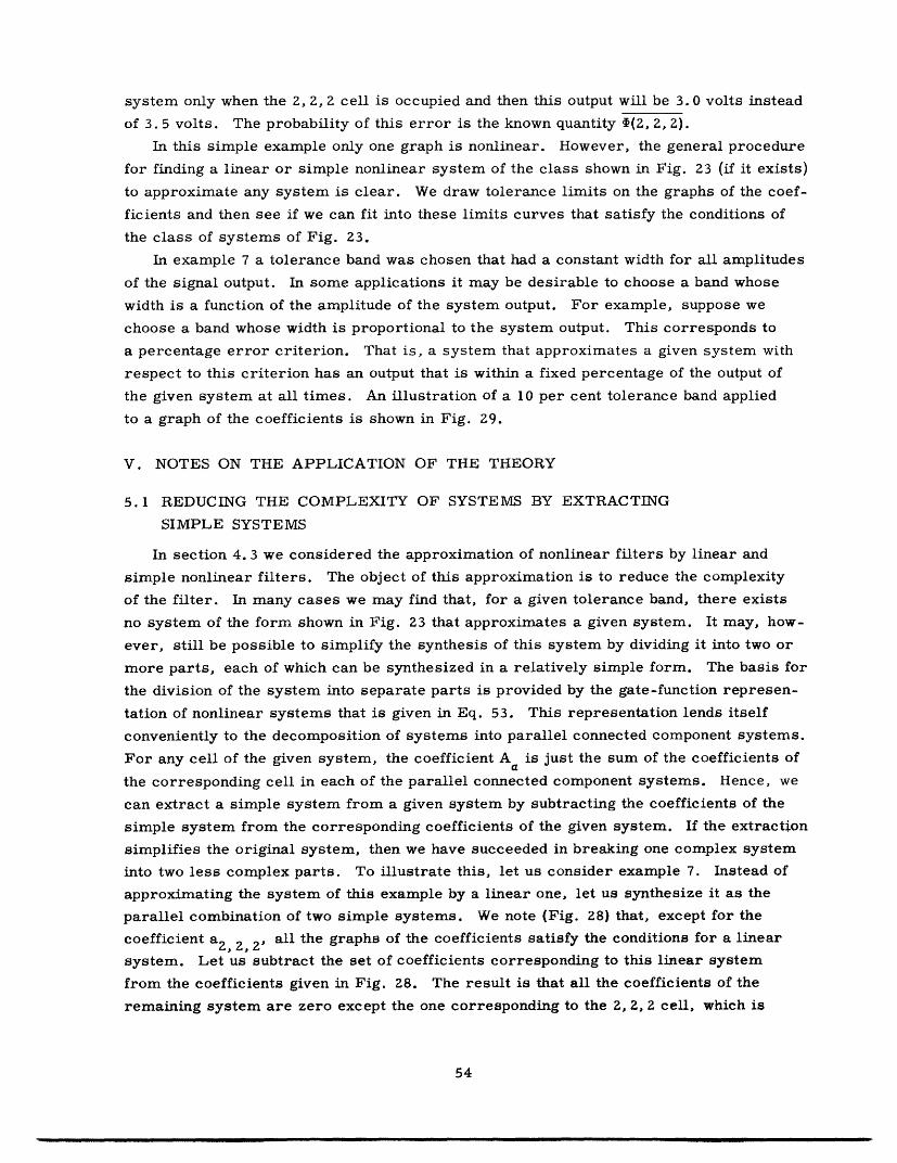
system only when the 2, 2, 2 cell is occupied and then this output will be 3.0 volts instead

of 3.5 volts. The probability of this error is the known quantity (2, 2, 2).

In this simple example only one graph is nonlinear. However, the general procedure

for finding a linear or simple nonlinear system of the class shown in Fig. 23 (if it exists)

to approximate any system is clear. We draw tolerance limits on the graphs of the coef-

ficients and then see if we can fit into these limits curves that satisfy the conditions of

the class of systems of Fig. 23.

In example 7 a tolerance band was chosen that had a constant width for all amplitudes

of the signal output. In some applications it may be desirable to choose a band whose

width is a function of the amplitude of the system output. For example, suppose we

choose a band whose width is proportional to the system output. This corresponds to

a percentage error criterion. That is, a system that approximates a given system with

respect to this criterion has an output that is within a fixed percentage of the output of

the given system at all times. An illustration of a 10 per cent tolerance band applied

to a graph of the coefficients is shown in Fig. 29.

V. NOTES ON THE APPLICATION OF THE THEORY

5.1 REDUCING THE COMPLEXITY OF SYSTEMS BY EXTRACTING

SIMPLE SYSTEMS

In section 4. 3 we considered the approximation of nonlinear filters by linear and

simple nonlinear filters. The object of this approximation is to reduce the complexity

of the filter. In many cases we may find that, for a given tolerance band, there exists

no system of the form shown in Fig. 23 that approximates a given system. It may, how-

ever, still be possible to simplify the synthesis of this system by dividing it into two or

more parts, each of which can be synthesized in a relatively simple form. The basis for

the division of the system into separate parts is provided by the gate-function represen-

tation of nonlinear systems that is given in Eq. 53. This representation lends itself

conveniently to the decomposition of systems into parallel connected component systems.

For any cell of the given system, the coefficient A is just the sum of the coefficients of

the corresponding cell in each of the parallel connected component systems. Hence, we

can extract a simple system from a given system by subtracting the coefficients of the

simple system from the corresponding coefficients of the given system. If the extraction

simplifies the original system, then we have succeeded in breaking one complex system

into two less complex parts. To illustrate this, let us consider example 7. Instead of

approximating the system of this example by a linear one, let us synthesize it as the

parallel combination of two simple systems. We note (Fig. 28) that, except for the

coefficient a 2 , 2, 2' all the graphs of the coefficients satisfy the conditions for a linear

system. Let us subtract the set of coefficients corresponding to this linear system

from the coefficients given in Fig. 28. The result is that all the coefficients of the

remaining system are zero except the one corresponding to the 2, 2, 2 cell, which is

54

0.5. The coefficients of the extracted linear system are those of example 6. Hence,

the nonlinear system of example 7 can be synthesized as the parallel combination of the

linear system of Fig. 27 and a very simple nonlinear system that has only one coefficient,

a, 2 2 = 0.5. This approach of extracting simple systems to reduce the complexity of

a system is effective only when, as in this example, the extraction causes many of the

coefficients of the remaining system to be zero, thereby simplifying its synthesis.

5.2 OPTIMIZATION OF THE LAGUERRE FUNCTION SCALE FACTOR

It has been assumed throughout that the scale factor associated with the argument

of the Laguerre functions is unity. By substituting kx for x in Eq. 1 we obtain the

Laguerre functions that have the scale factor k. But we have no convenient analytical

method for determining the optimum value of k in the filter problem. Recall that the

impulse response at the nth-output terminal of the Laguerre network is h (t) or hn(kt)

with the scale factor k. We see that k effects a time scaling of the impulse response

of the Laguerre network and hence a frequency scaling of the transfer function of this

network. In determining optimum filters by the methods that have been described we

can make use of our knowledge of the frequency band of x(t) to judiciously choose k.

It would be convenient, however, to have a method for obtaining the optimum k rather

than just a good guess for it. An experimental procedure for obtaining the optimum k

will now be described.

Consider the effect of changing the time scale of x(t) and z(t) in the experimental

procedure for determining optimum filters. That is, consider that these time functions

are replaced by x(t/k) and z(t/k). In the laboratory this could be achieved by recording

the ensemble members of x(t) and z(t) and then playing the recording back at a speed of

1/k times the recording speed. First, consider the effect of this time scaling on the

determination of no-storage filters in accordance with Fig. 9. It is clear that, since

the apparatus for determining the filters has no memory, its operation is independent

of the time scaling. That is, the same filter will be determined regardless of the value

of k. Now consider the procedure (Fig. 13) for determining optimum filters involving

memory. We notice that the only portion of the apparatus that involves memory is the

Laguerre network. As a consequence, if we replace x(t) and z(t) by x(t/k) and z(t/k),

we obtain the same filter as if we had used x(t) and z(t) but changed the scale factor

of the Laguerre network from unity to k. Now recall (sec. 3. 6) that apparatus can be

constructed that indicates the minimum error for the optimum filter (of the class of

filters with a given Laguerre network and generator). This apparatus, like that

shown in Fig. 13, consists of no-memory circuits and a Laguerre network. By varying

the speed of the recordings of x(t) and z(t) which are fed into this apparatus and observing

its output (min of Eq. 62) we can directly determine the optimum k. In practice, we

would build the Laguerre network in the minimum error detecting apparatus so that it

would have a scale factor corresponding to our judicious guess of the optimum k. Then

we could vary the speeds of the recordings of x(t) and z(t) in order to explore scale

55

- C 1_. -·1111�-L -1 -- - -�_

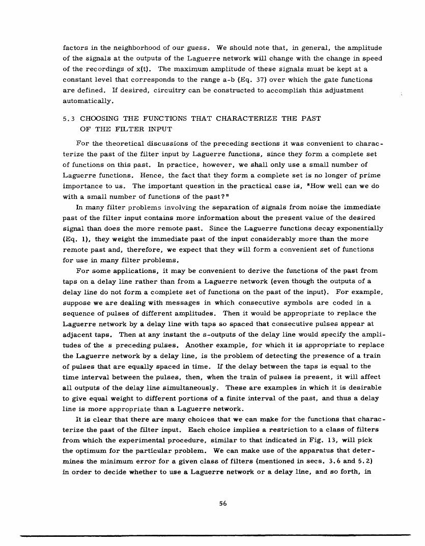
factors in the neighborhood of our guess. We should note that, in general, the amplitude

of the signals at the outputs of the Laguerre network will change with the change in speed

of the recordings of x(t). The maximum amplitude of these signals must be kept at a

constant level that corresponds to the range a-b (Eq. 37) over which the gate functions

are defined. If desired, circuitry can be constructed to accomplish this adjustment

automatically.

5.3 CHOOSING THE FUNCTIONS THAT CHARACTERIZE THE PAST

OF THE FILTER INPUT

For the theoretical discussions of the preceding sections it was convenient to charac-

terize the past of the filter input by Laguerre functions, since they form a complete set

of functions on this past. In practice, however, we shall only use a small number of

Laguerre functions. Hence, the fact that they form a complete set is no longer of prime

importance to us. The important question in the practical case is, "How well can we do

with a small number of functions of the past?"

In many filter problems involving the separation of signals from noise the immediate

past of the filter input contains more information about the present value of the desired

signal than does the more remote past. Since the Laguerre functions decay exponentially

(Eq. 1), they weight the immediate past of the input considerably more than the more

remote past and, therefore, we expect that they will form a convenient set of functions

for use in many filter problems.

For some applications, it may be convenient to derive the functions of the past from

taps on a delay line rather than from a Laguerre network (even though the outputs of a

delay line do not form a complete set of functions on the past of the input). For example,

suppose we are dealing with messages in which consecutive symbols are coded in a

sequence of pulses of different amplitudes. Then it would be appropriate to replace the

Laguerre network by a delay line with taps so spaced that consecutive pulses appear at

adjacent taps. Then at any instant the s-outputs of the delay line would specify the ampli-

tudes of the s preceding pulses. Another example, for which it is appropriate to replace

the Laguerre network by a delay line, is the problem of detecting the presence of a train

of pulses that are equally spaced in time. If the delay between the taps is equal to the

time interval between the pulses, then, when the train of pulses is present, it will affect

all outputs of the delay line simultaneously. These are examples in which it is desirable

to give equal weight to different portions of a finite interval of the past, and thus a delay

line is more appropriate than a Laguerre network.

It is clear that there are many choices that we can make for the functions that charac-

terize the past of the filter input. Each choice implies a restriction to a class of filters

from which the experimental procedure, similar to that indicated in Fig. 13, will pick

the optimum for the particular problem. We can make use of the apparatus that deter-

mines the minimum error for a given class of filters (mentioned in secs. 3.6 and 5.2)

in order to decide whether to use a Laguerre network or a delay line, and so forth, in

56

n

a given problem. We insert the different networks into this apparatus in place of the

Laguerre network and choose the one that yields the smallest error.

5.4 CHOOSING THE NUMBER OF GATE FUNCTIONS

By increasing the number of gate functions that are associated with each Laguerre

coefficient we quantize the function space of the input into smaller cells. While, in

general, this is desirable from the point of view of reducing the filtering error, it leads

to a very large number of coefficients that have to be evaluated. In applying the theory

we should, when possible, make use of any information about the particular filter

problem that will enable us to reduce the number of gate functions. For example, con-

sider the problem of pure (noiseless) prediction of a stationary time function consisting

of equally spaced pulses with amplitudes of zero or unity with a certain probability dis-

tribution. As we found in the previous section, it is appropriate, for a problem of this

kind, to replace the Laguerre network by a delay line. The output from each tap on the

delay line will then take on only the values zero and unity. Hence, we need only two

gate functions for each output of the delay line.

In the previous section we also mentioned that in many filter problems the immediate

past of the input contains more information about the present value of the desired output

than does the more remote past. A study of the Laguerre functions shows that the higher-

order functions weight the remote past more strongly than do the lower-order functions..

Hence, we expect that, for purposes of filtering, it might not be as important to distin-

guish small changes in the amplitude of the higher-order Laguerre coefficients as in the

lower-order ones (or, in the case of delay lines, it might not be as important to distin-

guish small changes in those outputs that represent samples of the more remote past).

Thus we might choose a smaller number of gate functions for the higher-order Laguerre

coefficients than for the lower-order ones.

In summary, the choices of the scale factor, the functions that characterize the past

of the input, and the number of gate functions are all choices that determine the class

of filters from which the procedure, similar to that indicated in Fig. 13, determines

the optimum filter. We should use any information about the particular filter problem

that will enable us to judiciously choose the class of filters so that the number of coef-

ficients is reasonable in the light of the task that the filter is to perform.

Acknowledgment

The author wishes to express his deep appreciation to Professor Y. W. Lee, who

first suggested a study of the Wiener theory of nonlinear system characterization and

supervised the research that resulted from this study. The constructive criticism of

Professor Lee in the research and in the writing of this report led the work to its present

form. The author is also indebted to Professor Norbert Wiener, who has been a source

of inspiration through his explanations and discussions of his theory.

57

_*___II___�___IIIIII�--·I�· Il�·l-Y�IIII11-ll�_ �

References

1. N. Wiener, Mathematical problems of communication theory, Summer SessionLecture Notes, 1953-1954, M.I.T. (unpublished).

2. Y. W. Lee, Synthesis of electric networks by means of the Fourier transformsof Laguerre's functions, J. Math. Phys. 2, 83-113 (June 1932).

3. E. C. Titchmarsh, Introduction to the Theory of Fourier Integrals (Oxford Univer-sity Press, London, 1937), pp. 76-82.

4. N. Wiener, The Fourier Integral and Certain of its Applications (Dover Publications,Inc., New York, 1933).

5. H. E. Singleton, Theory of nonlinear transducers, Technical Report 160, ResearchLaboratory of Electronics, M.I.T., Aug. 12, 1950, pp. 30-32.

6. Y. W. Lee, Statistical theory of communication, Course 6.563 Class Notes, 1952,M. I. T. (unpublished).

7. N. Wiener, Extrapolation, Interpolation, and Smoothing of Stationary Time Series(John Wiley and Sons, Inc., New York, 1949).

8. L. A. Zadeh, Optimum nonlinear filters for the extraction and detection of signals,a paper presented at the IRE National Convention, New York, March 25, 1953.

9. T. E. Stern, Piecewise-linear analysis and synthesis, a paper presented at theSymposium on Nonlinear Circuit Analysis II, Polytechnic Institute of Brooklyn,April 26, 1956.

58