A Theory of Procyclical Bank Herding1

Viral V. Acharya2

London Business School and CEPR

Tanju Yorulmazer3

Bank of England

J.E.L. Classification: G21, G28, G38, E58, D62.

Keywords: Systemic risk, Contagion, Herding,

Procyclicality, Information spillover, Inter-bank correlation

First Draft: September 15, 2002

This Draft: March 1, 2004

1This paper was earlier titled as “Information Contagion and Inter-Bank Correlation in a Theory of Systemic Risk.” We are grateful to Franklin

Allen and Douglas Gale for their encouragement and advice, to Luigi Zingales for suggesting that the channel of information spillovers be examined as

a source of systemic risk, to Sudipto Bhattacharya, Amil Dasgupta, Phillip Hartmann, John Moore, Raghu Sundaram, Anjan Thakor, Andy Winton,

and seminar participants at Bank of Canada, Bank of England, Bank for International Settlements, Center for Economic Policy Research (CEPR)

Conference on “Financial Stability and Monetary Policy,” Corporate Finance Workshop - London School of Economics, Department of Economics

- New York University, Federal Deposit Insurance Corporation (FDIC) Conference on “Finance and Banking: New Perspectives,” Financial Crises

Workshop conducted by Franklin Allen at Stern School of Business - New York University, International Monetary Fund, and London Business

School, for useful comments, and to Nancy Kleinrock for editorial assistance. All errors remain our own.

2Contact: Department of Finance, London Business School, Regent’s Park, London – NW1 4SA, England. Tel: +44 (0)20 7262 5050 Fax: +44

(0)20 7724 3317 e–mail: vacharya@london.edu. Acharya is also a Research Affiliate of the Centre for Economic Policy Research (CEPR).

3Contact: Financial Industry and Regulation Division, Bank of England, Threadneedle Street, London, EC2R 8AH, Tel: +44 (0) 20 7601 3198

Fax: +44 (0) 20 7601 3217 e–mail: Tanju.Yorulmazer@bankofengland.co.uk

A Theory of Procyclical Bank Herding

Abstract

When bank loan returns have a systematic factor, the failure of one bank conveys adverse

information about this systematic factor and increases the cost of borrowing for the surviv-

ing banks relative to the situation of no bank failures. Such information spillover is costly to

profit-maximizing bank owners. Given their limited liability, bank owners herd ex-ante and

undertake correlated investments to increase the likelihood of joint survival. Competitive ef-

fects such as superior margins from lending to different industries and migration of depositors

of a failed bank to the surviving bank mitigate herding incentives. When expected returns

on loans are low (economic booms), the herding incentives dominate, whereas when expected

returns are high (economic downturns), the competitive effects dominate. This gives rise to

a pro-cyclical pattern in the industry-based concentration of aggregate bank lending.

J.E.L. Classification: G21, G28, G38, E58, D62.

Keywords: Systemic risk, Contagion, Herding, Procyclicality, Information spillover, Inter-

bank correlation

1 Introduction

While it is well-known that the levels of bank lending vary in a procyclical manner (Borio,

Furfine and Lowe, 2001, Berger and Udell, 2002, and the references therein), recent empirical

evidence suggests that the concentration of aggregate bank lending also exhibits a procyclical

variation. Mei and Saunders (1997), for example, document that bank lending in the United

States to the real estate sector follows a procyclical or a “trend-chasing” pattern: returns

to investments in the real estate sector are mean-reverting whereas banks appear to lend

more to this sector when its past performance has risen above the trend. In more recent

evidence, Hoggarth and Pain (2002) document that the growth in bank loans to real estate

and construction sectors in the United Kingdom rises disproportionately in the boom period

of the economy: in the period December 1987 to December 1989, lending to these sectors grew

by 55% and 40% respectively, compared to around 25% for other sectors. Complementing this

evidence is the finding of Dell’Ariccia and Garibaldi (2003), which shows that the aggregate

bank credit reallocation (credit reshuffling in excess of net credit level changes) in the United

States is greater in downturns than in booms.

Why does the concentration of bank lending to certain sectors vary procylically even

though the returns to these sectors appear to be countercyclical? In this paper, we provide

an explanation for this phenomenon by building a theory that examines the interaction of

information contagion among banks with the ex-ante incentives of banks to herd. Also crucial

to our theory is the role of competitive benefits to banks from specialization (or differentiation)

such as superior margins in lending and migration of depositors of failed banks to surviving

banks. The trade-off between incentives to herd and to specialize is shown to depend on the

anticipated profitability of corporate sector, and in turn, delivers a procyclical variation in the

concentration of aggregate bank lending. We believe the model also lays down a foundation

for studying different forms of systemic risk in a unified setting.

In our model, there are two periods and two banks with access to risky loans and de-

posits. The returns on each bank’s loans consist of a systematic component, say a common

factor driving loan returns such as an aggregate or an industry cycle, and an idiosyncratic

component. The ex-ante structure of each bank’s loan returns, specifically their exposure to

systematic and idiosyncratic factors, is common knowledge; the ex-post performance of each

bank’s loan returns is also publicly observed. However, the exact realization of systematic

and idiosyncratic components is not observed by the economic agents. Ex-ante, banks choose

whether to lend to similar industries and thereby maintain a high level of inter-bank cor-

relation, or to lend to different industries. If banks lend to similar industries, their lending

margins are eroded relative to the margins they earn upon lending to different industries.

In the benchmark case, depositors of a bank do not receive any information other than

the performance of their own bank. In this case, banks choose the lowest possible level of

1

correlation in order to retain their profit margins. Next, we allow depositors to also receive

information about the performance of the other bank. The failure of each bank conveys

potential bad news about the common factor affecting loan returns. Similarly, the good

performance of each bank is good news about the common factor. Depositors rationally

update priors about the prospects of their bank based on the information received about not

only their bank’s returns but also of other banks. In particular, depositors require a higher

promised rate on their deposits if the other bank has failed compared to the state in which

both banks have survived. This is an information spillover of one bank’s failure on the other

bank’s borrowing costs, and in turn on its profits. Indeed, if the future profitability of loans

is low, the surviving bank cannot pay the borrowing rate when one bank fails though it can

pay this rate when no bank fails. We interpret this as an information contagion.

We argue that in order to minimize the impact of such spillover on profits, banks alter

their ex-ante investment choices. The greater the correlation between the loan returns of

banks, the greater is the likelihood that they will survive together; in turn, the lower is their

expected cost of borrowing in the future and higher are their expected profits. Consequently,

banks herd by lending to similar industries and increase inter-bank correlation (in excess of

the benchmark case where banks pick uncorrelated investments).1 Intuitively, banks prefer

to survive together rather than surviving individually. In the latter case, they face the risk

of information spillover. In contrast, given their limited liability, bank owners view failing

individually and failing together with other banks in a similar light.

As long as the effect of competition on bank margins is not too severe, the above intuition

prevails: banks herd completely, that is, they choose perfectly correlated investments, over a

robust set of parameter values for the future profitability of corporate sector. Incentives to

herd by lending to a common industry are thus stronger if there is a high concentration of

bank lending to that industry, or, if that industry has experienced a positive technology shock

reducing the rate at which returns-to-scale diminish. Such herding can lead to productive

inefficiency as banks bypass profitable projects in other industries of the economy.

However, herding incentives are weakened if the anticipated profitability of corporate

sector is sufficiently high. Intuitively, in the presence of competition, a given increase in the

future profitability of corporate sector leads to a greater increase in bank profits if they face

less competition in lending. This gives banks an incentive to specialize with respect to other

banks in terms of which industries they lend to. If depositors of the failed bank can migrate

to the surviving bank (a form of “flight to quality”), then there is an additional incentive for

banks not to herd.

To summarize, when the expected profitability of future lending business is low (the re-

1Note that this form of ex-ante herding is different from ex-post or sequential herding that arises in typicalinformation-based models of herd behavior. We elaborate on this difference in Section 8.1.

2

gion of business cycle peaks), banks shy away from situations where information spillover is

likely and herd, giving rise to high inter-bank correlation. In contrast, when the expected

profitability of future lending business is high (the region of business cycle troughs), herding

incentives are weakened by prospects of large future profits and the level of inter-bank corre-

lation is reduced. We interpret this phenomenon as procyclicality of bank herding consistent

with the observed procyclicality in concentration of aggregate bank lending. An increase

in the likelihood of economic downturn, again a characteristic of business cycle peaks, also

accentuates herding incentives.

This result on the procyclicality of bank herding incentives is an important and novel

contribution of the paper. While existing theories of bank herding have largely relied on

managerial reputation considerations (see, for example, Rajan 1994), we show that even

profit-maximizing managers (bank owners) may engage in herding. In the managerial herding

literature, relative performance evaluation generates herding behavior: managers can “share

the blame” when they underperform together. In our model, information spillover and limited

liability of banks combine in generating herding behavior: banks can capitalize on reduced

borrowing costs when they have a good performance together. In particular, banks herd even

in the absence of any managerial agency problems.

Section 2 discusses the related literature. Section 3 presents the model. Section 4 analyzes

the benchmark case where there is no information spillover. Section 5 introduces information

spillover, and delivers the results on procyclical herding. Section 6 examines the productive

inefficiency resulting from bank herding. Section 7 considers an extension with more than two

banks and heterogeneity among banks in systematic factor exposures. Section 8 relates our

work to managerial herding, inter-bank linkages, and regulatory issues. Section 9 concludes.

Proofs not contained in the main text are in the Appendix.

2 Related Literature

Several aspects of our model have roots in the documented empirical facts about banking

crises. Below we summarize the literature that is most relevant to this paper.

The empirical studies on bank contagion test whether bad news, such as a bank failure,

the announcement of an unexpected increase in loan-loss reserves, bank seasoned stock issue

announcements, etc., adversely affect the other banks.2 These studies have concentrated on

2If the effect is negative, the empirical literature calls it the “contagion effect.” The overall finding isthat the contagion effect is stronger for highly leveraged firms (banks being typically more levered thanother industries) and is stronger for firms with similar cash flows. If the effect is positive, it is termed the“competitive effect.” The intuition is that demand for the surviving competitors’ products (deposits, in thecase of banks) can increase. Overall, this effect is found to be stronger when the industry is less competitive.

3

various indicators of contagion, such as the intertemporal correlation of bank failures (Hasan

and Dwyer 1994, Schoenmaker 1996), bank debt risk premiums (Carron, 1982, Saunders,

1987, Karafiath, Mynatt, and Smith, 1991, Jayanti and Whyte, 1996), deposit flows (Saun-

ders, 1987, Saunders and Wilson, 1996, Schumacher, 2000), survival times (Calomiris and

Mason, 1997, 2000), and stock price reactions (as discussed below). Most empirical investi-

gations of bank contagion are event studies of bank stock price reactions in response to bad

news concerning other banks. These studies3 generally find significant negative abnormal

returns, regard this as evidence for contagion, and conclude that such reactions are rational

investor choices in response to newly revealed information, as suggested also by Gorton (1988)

and Calomiris and Gorton (1991), rather than purely panic-based contagion, as modeled in

Diamond and Dybvig (1983).

Chari and Jagannathan (1988) and Jacklin and Bhattacharya (1988) model information-

based bank runs wherein a depositor’s decision to run on a bank may lead other depositors

to run, either on the same bank or on others. Our model of information contagion is closer

to the recent models of Chen (1999) and Kodres and Pritsker (2002). Chen (1999) extends

the Diamond-Dybvig model to multiple banks with interim revelation of information about

some banks. With Bayesian-updating depositors, a sufficient number of interim bank failures

results in pessimistic expectations about the general state of the economy, and leads to runs

on the remaining banks. In contrast, in our model the information spillover shows up in

both increased borrowing rates and also in bank failures – an aspect that relates better to

the empirical evidence. Kodres and Pritsker (2002) allow for different channels for financial

markets contagion including the correlated information channel. They show how contagion

can occur between markets due to cross-market rebalancing even in the absence of correlated

information and liquidity shocks. In contrast, contagion in our paper results necessarily from

the correlated information channel. Furthermore, these papers do not model the endogenous

choice of correlation of banks’ investments. On this front, our paper is closest in spirit

to Acharya (2000) who examines the choice of ex-ante inter-bank correlation in response

to financial externalities that arise upon bank failures and in response to “too-many-to-

fail” regulatory guarantees. The channel of information spillover that we examine however

complements the channels examined in Acharya (2000).

Finally, our paper is related to the vast literature on herding. We relegate to Section 8.1

a detailed discussion of this relationship.

3See Aharony and Swary (1983), Waldo (1985), Cornell and Shapiro (1986), Saunders (1986), Swary(1986), Smirlock and Kaufold (1987), Peavy and Hempel (1988), Wall and Peterson (1990), Gay, Timme andYung (1991), Karafiath, Mynatt, and Smith (1991), Madura, Whyte, and McDaniel (1991), Cooperman, Lee,and Wolfe (1992), Rajan (1994), Jayanti and Whyte (1996), Docking, Hirschey, and Jones (1997), Slovin,Sushka, and Polonchek (1992) and (1999), Lang and Stulz (1992).

4

3 Model

There are two banks in the economy, Bank A and Bank B, and three dates, t = 0, 1, 2.

The timeline in Figure 1 details the sequence of events in the economy. There is a single

consumption good at each date. Each bank can borrow competitively from a continuum of

risk-averse depositors of measure 1. Depositors consume their each-period payoff (say, w)

and obtain time-additive utility u(w), with u′(w) > 0, u′′(w) < 0, ∀w > 0, and u(0) = 0.

Depositors have one unit of the consumption good at t = 0 and t = 1. Banks are owned by

financial intermediaries, henceforth referred to as bank owners. Bank owners are risk-neutral

and also consume their each-period payoff.

All agents have access to a storage technology that transforms one unit of the consumption

good at date t to one unit at date t + 1. In each period, that is at date t = 0 and t =

1, depositors choose to keep their good in storage or to invest it in their bank. Deposits

take the form of a simple debt contract with maturity of one period. In particular, the

promised deposit rate is not contingent on realized bank returns. Furthermore, since bank

investment decisions are assumed to be made after deposits are borrowed, the promised

deposit rate cannot be contingent on these investment decisions. Finally, the dispersed nature

of depositors is assumed to lead to a collective-action problem, resulting in a run on a bank

that fails to pay the promised return to its depositors. In other words, the contract is “hard”

and cannot be renegotiated.

Banks choose to invest the borrowed goods in storage or in a risky asset. The risky asset

is to be thought of as a portfolio of loans to firms in the corporate sector. The performance

of a bank’s loan portfolio is determined by the random output of its borrowers at date t + 1 :

either the output is High and there is correspondingly a high return on the bank portfolio,

or the output is Low and there is default on bank loans. In case of default, we assume that

for simplicity there is no repayment on bank loans.

This return on bank investments depends on a systematic component, a common factor

affecting loan returns, and an idiosyncratic component. We refer to the common factor as the

overall state of the economy, which can be Good(G) or Bad(B), recognizing that it represents

more broadly any common component of loan returns (such as a sector-specific or a regional

component) that is not perfectly observable. Given that a proportion of bank loans is in

fact to small- and medium-sized firms, usually unrated by rating agencies, we believe the

assumption that such an unobservable common factor exists is a reasonable one. The state

of the economy persists for both periods of the economy.

The prior probability that the state is Good for the risky asset is p. However, if the overall

state of the economy is good (bad), the return can be low (high) due to the idiosyncratic

component. The probability of a high return on bank investments when the state is good is

5

state\return High Low

Good pq p(1− q)

Bad (1− p)(1− q) (1− p)q

Table 1: Joint probabilities of returns and states for an individual bank.

Bank A\Bank B High Low

High SS SF

Low FS FF

Table 2: Possible outcomes from first period investments.

q ∈ (12

, 1): when the state is good, it is more likely, although not certain, that the return will

be high. The probability that the return is high when the state is bad is (1− q). Therefore,

the probability distributions of returns in different states are symmetric. The resulting joint

probabilities of the states and bank returns are given in Table 1. For simplicity, we assume

that, conditional on the state of the economy, the realizations of returns in the first and second

period are independent. While we allow the promised returns on bank loans to depend upon

t and thus vary over time, for simplicity we do not explicitly index them to the state of the

economy.

We assume that if the return from the first period investment is low for a bank, then there

is a run on the bank, it is liquidated and it cannot operate any further. If the return is high,

then bank owners make the second-period investment. Therefore the possible cases at date

1 are given as follows (Table 2), where S indicates survival and F , failure:

SS : Both banks had the high return, and they operate in the second period.

SF : Bank A had the high return, while Bank B had the low return. Only Bank A operates

in the second period. Bank B depositors invest their second-period goods in storage.

FS : This is the symmetric version of state SF .

FF : Both banks failed. No bank operates in the second period.

3.1 Correlation of Bank Returns

Banks can choose the level of correlation between the returns from their respective investments

by choosing the composition of loans that compose their respective portfolios. We will refer

to this correlation as “inter-bank correlation” and denote it as ρ ∈ [0, 1].4

4In order to focus exclusively on the choice of inter-bank correlation, we abstract from the much-studiedissue of the banks’ choice of the scale of their loan portfolios and their absolute level of risk. This abstractionis common to several papers in this literature including the ones on herding due to managerial reputation

6

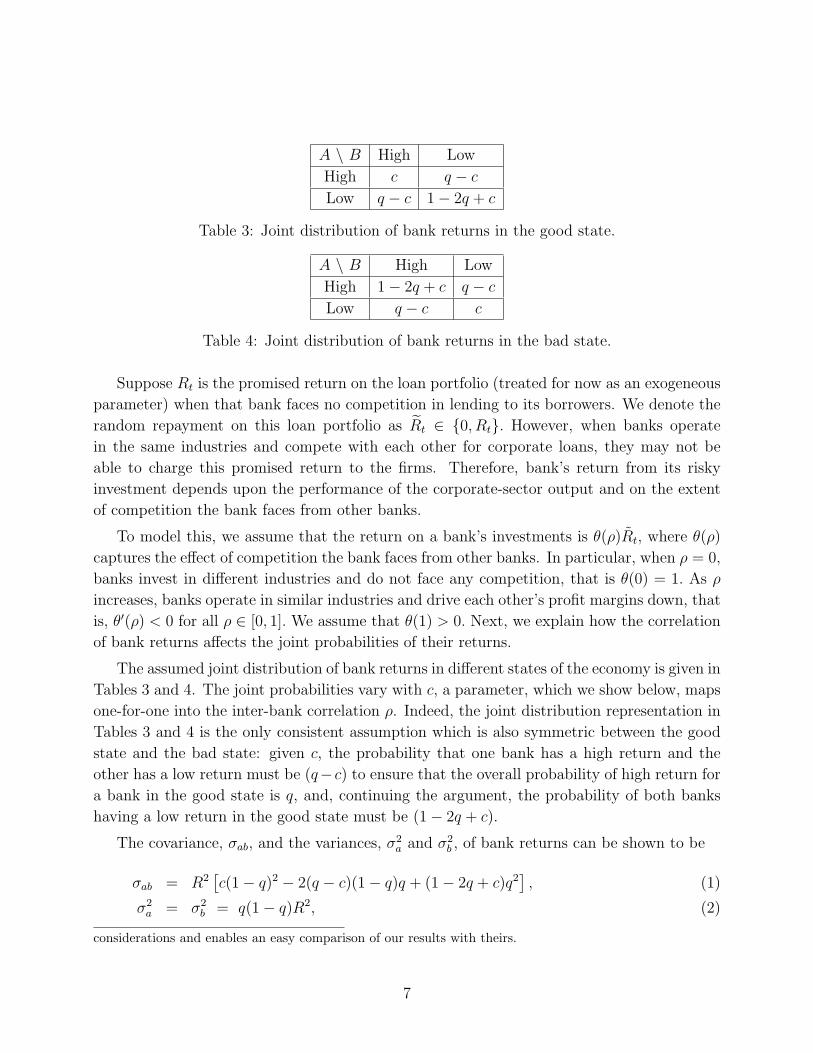
A \ B High Low

High c q − c

Low q − c 1− 2q + c

Table 3: Joint distribution of bank returns in the good state.

A \ B High Low

High 1− 2q + c q − c

Low q − c c

Table 4: Joint distribution of bank returns in the bad state.

Suppose Rt is the promised return on the loan portfolio (treated for now as an exogeneous

parameter) when that bank faces no competition in lending to its borrowers. We denote the

random repayment on this loan portfolio as Rt ∈ {0, Rt}. However, when banks operate

in the same industries and compete with each other for corporate loans, they may not be

able to charge this promised return to the firms. Therefore, bank’s return from its risky

investment depends upon the performance of the corporate-sector output and on the extent

of competition the bank faces from other banks.

To model this, we assume that the return on a bank’s investments is θ(ρ)Rt, where θ(ρ)

captures the effect of competition the bank faces from other banks. In particular, when ρ = 0,

banks invest in different industries and do not face any competition, that is θ(0) = 1. As ρ

increases, banks operate in similar industries and drive each other’s profit margins down, that

is, θ′(ρ) < 0 for all ρ ∈ [0, 1]. We assume that θ(1) > 0. Next, we explain how the correlation

of bank returns affects the joint probabilities of their returns.

The assumed joint distribution of bank returns in different states of the economy is given in

Tables 3 and 4. The joint probabilities vary with c, a parameter, which we show below, maps

one-for-one into the inter-bank correlation ρ. Indeed, the joint distribution representation in

Tables 3 and 4 is the only consistent assumption which is also symmetric between the good

state and the bad state: given c, the probability that one bank has a high return and the

other has a low return must be (q−c) to ensure that the overall probability of high return for

a bank in the good state is q, and, continuing the argument, the probability of both banks

having a low return in the good state must be (1− 2q + c).

The covariance, σab, and the variances, σ2a and σ2

b , of bank returns can be shown to be

σab = R2[c(1− q)2 − 2(q − c)(1− q)q + (1− 2q + c)q2

], (1)

σ2a = σ2

b = q(1− q)R2, (2)

considerations and enables an easy comparison of our results with theirs.

7

where the time subscript has been suppressed. Hence, the correlation of bank returns is

ρ =σab

σaσb

=c(1− q)2 − 2(q − c)(1− q)q + (1− 2q + c)q2

q(1− q)

=c

q(1− q)− q

1− q. (3)

It follows that ∂ρ∂c

= 1q(1−q)

> 0. We assume c ∈ [q2, q] that gives us ρ ∈ [0, 1].

Inter-bank correlation ρ is a joint choice of the banks which could be interpreted as the

outcome of a co-operative game between banks. In our model, this joint choice of inter-bank

correlation is identical to the one that arises from the Nash equilibrium choice of industries

by banks playing a coordination game.5

4 Benchmark Case: No Information Spillover

In the benchmark case, depositors observe only their own bank’s past return. As a result,

there is no information spillover between banks. Also, when a bank fails, its depositors

simply invest in storage in the next period. In particular, depositors do not migrate to the

surviving bank (if any), an assumption which does not affect the analysis in this benchmark

case. Though the benchmark case may not be a perfect representation of the real world, it

helps us isolate the effect of information spillover on banks’ choice of correlation. While the

choice of inter-bank correlation is determined by backwards induction, it is easier for sake of

exposition to first examine the investment problem at date 0.

4.1 First Investment Problem (date 0)

In the first period, both banks are identical. Hence, we consider a representative bank. Since

depositors have access to the storage technology, their individual rationality requires that the

bank offers a promised return r0 that gives depositors their reservation utility u(1), assumed

5For example, suppose that there are two possible industries in which banks can invest, denoted as 1 and2. Bank A (B) can lend to firms A1 and A2 (B1 and B2) in industries 1 and 2, respectively. If in Nashequilibrium banks choose to lend to firms in the same industry, specifically they either lend to A1 and B1,or they lend to A2 and B2, then they are perfectly correlated. However, if they choose different industries,then their returns are less than perfectly correlated, say independent. Allowing for a choice between severalindustries in the coordination game can produce a spectrum of possible inter-bank correlations (withoutaffecting the total risk of each bank’s portfolio). We do not adopt this modeling strategy for most of ourexposition since it sacrifices parsimony. Instead, we directly consider the joint choice of inter-bank correlationby banks. In the welfare analysis (Section 6), we do employ the coordination game formulation with only twoindustries, which by implication gives rise to two possible values for inter-bank correlation.

8

to be 1. Since r0 ≥ 1, it is straightforward to show that it is never optimal for banks to

invest in the safe asset. Given their limited liability, banks maximize their equity “option”

by investing all borrowed goods in the risky asset.6

Thus, depositors are paid the promised return r0 only if the return on bank loans is high.

Because of the limited liability of banks, depositors get nothing when the return on bank

loans is low. The probability of a high return on bank loans, denoted as α0, is

α0 = Pr(G) Pr(R0|G) + Pr(B) Pr(R0|B) = pq + (1− p)(1− q). (4)

The promised return r0 is thus given by α0 u(r0) = 1, or

r0 = u−1(1/α0). (5)

We assume that θ(1)R0 > r0, as otherwise the problem at hand is rendered uninteresting.

The payoff to the bank at date 1 from the first period investment, denoted as π1(ρ), is thus

given by

π1(ρ) =

{θ(ρ)R0 − r0 if R0 = R0

0 if R0 = 0. (6)

The expected payoff to the bank at date 0 from its first-period investment, E(π1(ρ)), is thus

E(π1(ρ)) = α0[θ(ρ)R0 − r0]. (7)

Note that this first-period expected payoff is decreasing in the inter-bank correlation.

4.2 Second Investment Problem (date 1)

Recall our simplifying assumption that realizations of returns in the first and second periods

are independent, conditional on the true state of the economy. However, depositors have

more information at t = 1 than they had at t = 0 to judge the profitability of the risky

asset in which their bank invests. Since there is a systematic component in the probabilities

of returns which lasts for both periods, the bank’s past return is relevant information and

depositors rationally update their beliefs in response to this information. In the benchmark

case, depositors can only observe their own bank’s performance. Thus, their posterior belief

6Formally, suppose the bank invests β units in the safe asset and (1−β) units in the risky asset. Then thepayoff in the next period is β + (1− β)R. In the low state, this payoff equals β which must be lower than r0,the promised amount to depositors, since r0 ≥ 1. Hence, bank owners receive no payoff in this case. In thehigh state, the bank’s payoff is β + (1− β)R. Hence, bank owners receive max[R − r0 − β(R − 1), 0], whichis decreasing in β. Since bank owners are risk-neutral and consume each period’s payoff, they always chooseβ = 0.

9

is the same when both banks survived (SS) and when only their own bank survived (SF ).

When a bank has the low return, it is liquidated, does not operate in the second period and

thus has a total return of 0 in both states FF and FS.

Observing the survival of their own bank in the first period (S), depositors update the

probabilities about the overall state of the economy using Table 1, to obtain

Pr(G|S) =Pr(G and S)

Pr(S|G) Pr(G) + Pr(S|B) Pr(B)=

pq

pq + (1− p)(1− q), and (8)

Pr(B|S) =(1− p)(1− q)

pq + (1− p)(1− q). (9)

Using these, depositors calculate the probability of a high return for their bank in the second

period, denoted as αs1, as

αs1 = Pr

(R1 = R1|S

)= Pr(G|S) Pr(R1 = R1|G) + Pr(B|S) Pr(R1 = R1|B)

=pq

pq + (1− p)(1− q)q +

(1− p)(1− q)

pq + (1− p)(1− q)(1− q)

=pq2 + (1− p)(1− q)2

pq + (1− p)(1− q). (10)

By the individual rationality of depositors, we obtain that

rs1 = u−1(1/αs

1). (11)

Note that αs1 does not depend on the inter-bank correlation ρ.

Given limited liability, the payoff to each bank at date 2 from the second-period invest-

ment, denoted as πs2(ρ), is given by

πs2(ρ) =

θ(ρ)R1 − rs

1 if SS and R1 = R1 and θ(ρ)R1 > rs1

R1 − rs1 if SF and R1 = R1 and R1 > rs

1

0 otherwise.

(12)

Though the depositors cannot condition the interest they demand from their bank on

the other bank’s performance, the promised loan rate the bank can charge to the borrowing

firms depends on whether the other bank operates in the second period or not. If both banks

operate in the second period (SS), then due to competition they can only charge θ(ρ)R1 for

the loans. However, if only one bank operates (SF ), then that bank can charge its borrowers

the rate R1.

Note that if θ(ρ)R1 < rs1, then it is individually rational for depositors not to lend their

goods to banks. Storage is preferred to deposits, since the highest return on loans is insuffi-

cient to compensate depositors for the risk of bank failure.

10

4.3 Choice of Inter-Bank Correlation

The objective of each bank is to choose the level of inter-bank correlation ρ at date 0 that

maximizes

E(π1(ρ)) + E(π2(ρ))

where discounting has been ignored since it does not affect any of the results. We can write

each bank’s problem as

maxρ∈[0,1]

Pr(R0) [θ(ρ)R0 − r0] + Pr(R1, SS) [θ(ρ)R1 − rs1]

+ + Pr(R1, SF ) [R1 − rs1]

+

where x+ = max(x, 0) and

Pr(R1, SF ) = Pr(G) Pr(R1, SF |G) + Pr(B) Pr(R1, SF |B)

= p(q − c)q + (1− p)(q − c)(1− q)

= (q − c) [pq + (1− p)(1− q)] , and (13)

Pr(R1, SS) = Pr(G) Pr(R1, SS|G) + Pr(B) Pr(R1, SS|B)

= pcq + (1− p)(1− 2q + c)(1− q). (14)

We assume below that θ(1)R1 > rs1 whereby θ(ρ)R1 > rs

1 for all ρ, and, in particular,

R1 > rs1. The analysis follows similarly for the case where θ(1)R1 ≤ rs

1. We can rewrite the

bank’s problem as

maxρ∈[0,1]

Pr(R0) [θ(ρ)R0 − r0] + [Pr(R1, SS) θ(ρ)R1 + Pr(R1, SF ) R1]− Pr(R1, S) rs1

where Pr(R1, S) = Pr(R1, SS)+Pr(R1, SF ) = pq2 +(1−p)(1−q)2. This probability does not

depend on c, and in turn, does not depend on ρ. The probability Pr(R0) and the promised

interest rates r0 and rs1 are also independent of the level of correlation ρ. The returns from the

loans, θ(ρ)R0 and θ(ρ)R1, decrease as the level of correlation increases. Finally, note that as ρ

increases, Pr(R1, SS) increases, therefore, [Pr(R1, SS) θ(ρ)R1 + Pr(R1, SF ) R1] decreases as

well. As a result, bank’s expected profits fall as the correlation rises. This is our benchmark

result:

Proposition 1 In the absence of information spillover, banks choose the lowest level of cor-

relation: ρ = 0.

11

5 Case with Information Spillover

In this section, we allow depositors to observe both banks’ past performance. Since bank

returns are subject to the same systematic component, the performance of the other bank

is also valuable for depositors in updating their beliefs about their own bank’s profitability.

This is a more realistic representation of the banking system and allows us to investigate the

role of information spillover on the choice of asset correlation.

Note that the first investment problem is exactly the same as the benchmark case. There-

fore we concentrate on the second investment problem.

5.1 Second Investment Problem (date 1)

Both banks survived (SS): In this case, both banks operate for another period. With

the information of the survival of both banks in the first period, depositors can update the

probabilities about the overall state of the economy using Tables 3 and 4, to obtain

Pr(G|SS) =Pr(G and SS)

Pr(SS|G) Pr(G) + Pr(SS|B) Pr(B)=

pc

pc + (1− p)(1− 2q + c)

=pc

(1− 2q)(1− p) + c, and (15)

Pr(B|SS) =(1− p)(1− 2q + c)

(1− 2q)(1− p) + c. (16)

Using these, depositors can calculate the probability of a high return for their bank in the

second period, denoted as αss1 , as

αss1 = Pr

(R1 = R1|SS

)= Pr(G|SS) Pr(R1 = R1|G) + Pr(B|SS) Pr(R1 = R1|B)

=pc

(1− 2q)(1− p) + cq +

(1− p)(1− 2q + c)

(1− 2q)(1− p) + c(1− q)

=pcq + (1− p)(1− q)(1− 2q + c)

(1− 2q)(1− p) + c. (17)

By the individual rationality of depositors, we obtain that

rss1 = u−1(1/αss

1 ). (18)

Since αss1 depends on c, it is a function of the inter-bank correlation ρ. We denote this

borrowing rate as rss1 (ρ).

12

Thus, the payoff to each bank at date 2 from the second period investment, denoted as

πss2 , is given by

πss2 (ρ) =

{θ(ρ)R1 − rss

1 (ρ) if R1 = R1 and θ(ρ) R1 > rss1 (ρ)

0 otherwise.(19)

Note that if θ(ρ)R1 < rss1 (ρ), then it is individually rational for depositors not to lend their

goods to banks and instead invest in storage.

Only one bank survived (SF or FS): Without loss of generality, we concentrate on the

case SF where Bank A had a high return. From the symmetry of the joint probabilities in

different states and using Tables 3 and 4, we obtain

Pr(G|SF ) = p. (20)

Essentially, the good news about the economy from the performance of bank A is annulled by

the bad news from the failure of bank B. Excepting the possibility that R1 6= R0 in general,

this case is the same as the first-investment problem where the only information was the prior

belief about the overall state of the economy. Therefore,

rsf1 = u−1(1/α0) = r0. (21)

Observe that while the level of inter-bank correlation ρ affects the cost of borrowing in

the joint survival state, it does not affect the cost of borrowing in the individual survival

state. Also note that the surviving bank does not experience any competition and can earn

the return R1 from the corporate sector. Thus, in this case the payoff to the bank at date 2

from the second period investment, denoted πsf2 , is given by

πsf2 =

{R1 − r0 if R1 = R1 and R1 > r0

0 otherwise.(22)

5.2 Information Spillover

We can now characterize the spillover from the failure of a bank on the surviving bank. The

surviving bank’s cost of borrowing is higher relative to the state where both banks survive. It

is also higher relative to the benchmark case where other bank’s information is not available to

depositors. This is a negative spillover of a bank’s failure; or, put another way, the survival

of a bank results in a positive spillover on other surviving banks by lowering the cost of

borrowing. This tends to reduce the profits of banks in states where they survive but their

peers fail. In fact, if the profitability of the surviving bank’s investments (level of promised

13

return on loans R1) is low enough, the increased borrowing cost can render the surviving

bank unviable: depositors “run” on the surviving bank in response to other bank’s failure

since it is better for them to invest in storage than to lend to their bank. The result is an

“information contagion.”7 We use the word “contagion” even though we have only two banks

in our setting since the spillover to the surviving bank is similar in spirit to a contagion

with more than two banks. Furthermore, we examine a setting with more than two banks in

Section 7 where we argue that a similar spillover may arise for an entire group of banks.

Proposition 2 (Information Spillover) ∀ p, q, and ρ ∈ [0, 1],

rss1 (ρ) 6 rss

1 (1) = rs1 < rsf

1 = r0. Furthermore, rss1 (ρ) is increasing in ρ.

Note that the return depositors demand in state SS increases as the correlation in banks’

investments increases (Lemma A.1 in the Appendix). The reason for this is the following:

as correlation increases, the other bank’s high performance when depositors’ own bank has

performed well does not reveal much additional information. In the extreme case where banks

are perfectly correlated, ρ = 1, both banks’ performance will be identical and observing the

other bank’s performance will reveal no additional information: rss1 (1) = rs

1.

In the model, at date 0, there is no information about the overall state of the economy

and state SF reveals no additional information either. However, Proposition 2 suggests that

if a period of good news for the banking sector in general is followed by bad news for a few

banks, then other banks’ profits and values could fall due to an increase in the borrowing costs

(rss1 > rsf

1 ). Much empirical evidence exists to support such rational updating by depositors

and the resulting information spillover on bank values. We focus on a few representative

papers (see also Section 2).

Slovin, Sushka, and Polonchek (1992) examine share-price reactions to the announcements

of seasoned stock issues by commercial banks. They document significant negative effects

(−0.6%) on rival commercial and investment banks. In another study, Slovin, Sushka, and

Polonchek (1999) investigate 62 dividend reductions and 61 regulatory enforcement action

announcements over the period 1975–1992. They find that actions against money center

banks had negative contagion-type externality for other money center banks.

Lang and Stulz (1992) investigate the effect of bankruptcy announcements on the equity

value of the bankrupt firm’s competitors. They find that bankruptcy announcements decrease

7It is plausible that banks increase their lending rates when faced by an increased borrowing cost. However,this would ration the bank’s borrowers with project returns that are lower than the lending rate offered bythe bank. Providing that a bank cannot undo completely the decrease in its profits from increased borrowingrates by increasing its lending rates, this result on information contagion holds. We consider this scenarioreasonable, given the typical diminishing returns to scale faced by banks on lending side. See ample empiricalevidence in the discussion following Proposition 2 that supports the information contagion story.

14

the value of a value-weighted portfolio of competitors by 1%, the effect being stronger for

highly leveraged industries (banks being the primary candidate) and for firms exhibiting

substantial similarities. This they attribute to a contagion effect.

Rajan (1994) examines the effects of an announcement on December 15, 1989, that Bank

of New England was hurt from the poor performance of the real estate sector and that it

would boost its reserves to cover bad loans. He documents significant negative abnormal

returns (−2.4%) for all banks, and that the effect was stronger for banks with headquarters

in New England (−8%). He also documents significant negative abnormal returns for the

real estate firms in general, whereas the negative effect is stronger for real estate firms with

holdings in New England. This suggests that the announcement revealed information about

the real estate sector and more so about the real estate sector in New England, and that this

information was rationally taken into account by investors in their updating process.

Before exploring the consequences of such information contagion for the endogenous choice

of inter-bank correlation at date 0, the following computation of the expected payoff of banks

from their second-period investment is required. The ex-ante expected second-period return

of bank A (and by symmetry, of bank B) is given by

E(π2(ρ)) = Pr(R1, SS) [θ(ρ)R1 − rss1 (ρ)]+ + Pr(R1, SF ) (R1 − rsf

1 )+, (23)

where the expressions for Pr(R1, SF ) and Pr(R1, SS) are given in equations (13) and (14),

respectively. We assume henceforth that θ(1)R1 > rss1 (1), which ensures that banks are

viable in the state SS, ∀ ρ. This follows because rss1 (ρ) is increasing in ρ (Lemma A.1 in the

Appendix) and θ(ρ) is decreasing in ρ.

5.3 Choice of Inter-Bank Correlation

In this section, we show that under some conditions banks choose to be perfectly correlated

at date 0 in response to the anticipated information spillover at date 1 when banks fail. If

banks survive together, they subsidize each other’s borrowing costs. To capitalize on this,

banks prefer to invest in assets correlated with those of other banks, for example, by lending

to similar industries or geographic regions.

The objective of each bank is to choose the level of inter-bank correlation ρ that maximizes

E(π1(ρ)) + E(π2(ρ))

where E(π1(ρ)) equals Pr(R0) [θ(ρ)R0 − r0] and E(π2(ρ)) is given by equation (23).

Suppose that θ(ρ) = 1 − δρ with δ ∈ [0, 1). Note that this specification satisfies the

previous assumptions: θ(0) = 1, θ′(ρ) = −δ < 0 and θ(1) = 1 − δ > 0. Then, we obtain the

following result on ex-ante herding by banks.

15

Proposition 3 (Herding) ∃ δ∗ and maps R∗1(δ) and R∗∗

1 (δ) such that ∀ δ < δ∗, R∗1(δ) ≤

r0 < R∗∗1 (δ), and

(i) ∀ R1 ∈ [R∗1(δ), R

∗∗1 (δ)), banks choose to be perfectly correlated, that is, ρ = 1;

(ii) ∀ R1 ≥ R∗∗1 (δ), banks choose correlation ρ < 1 and this correlation decreases in R1.

Furthermore, R∗∗1 (δ) →∞ as δ → 0, and R∗∗

1 (δ) is decreasing in δ.

That is, if competition amongst banks in lending to a common set of industries does not

erode their lending margins too rapidly, then herding occurs over a robust set of parameter

values for the second-period profitability of these industries.8 In fact, we show in the Appendix

that even when R1 < R∗1(δ), the equilibrium value of ρ diminishes from 1 to 0 as R1 declines,

so that its level still exceeds the equilibrium level in the benchmark case with no information

spillover (ρ = 0).

While the proof of this proposition can be found in the Appendix, we provide an intuitive

explanation of our result based on the special case where δ = 0, that is, θ(ρ) = 1 for all

ρ ∈ [0, 1]: competition does not have any effect on bank loan returns.

First consider the case where θ(ρ) = 1 and R1 ≥ r0. Since there is no competition, E(π1)

is independent of ρ. Thus, banks would choose to be perfectly correlated provided E(π2(ρ))

in equation (23) is increasing in ρ. For the economy studied thus far, this condition holds

always: as we argue below, the expected cost of attracting depositors in the second period is

minimized when banks are perfectly correlated.

We can rewrite expected second-period profits as

E(π2(ρ)) =[pq2 + (1− p)(1− q)2

][R1 − (λ(ρ)rss

1 (ρ) + (1− λ(ρ))r0)] , where (24)

λ(ρ) =pcq + (1− p)(1− q)(1− 2q + c)

pq2 + (1− p)(1− q)2, (25)

and c is positively related to ρ as in equation (3). That is, the expected second-period profits

are the expected return on bank loans minus the expected borrowing cost in the second

period. This expected borrowing cost is a weighted average of the costs of borrowing in

the states SS and SF , that is, rss1 (ρ) and r0, with the respective weights being λ(ρ) and

(1 − λ(ρ)). These weights, up to a constant, are simply the probabilities of being in the

states SS and SF , respectively. Thus, the expression above makes it clear that the level of

inter-bank correlation enters the expected return of a bank through the promised interest

rates and through the probabilities of joint and individual survival states.

8If each bank chooses from one of two possible industries to lend to, then Proposition 3 would imply thatover the range R1 ∈ [R∗

1(δ), R∗∗1 (δ)), banks choose to lend to the same industry, and above the critical value

R∗∗1 (δ), banks start differentiating or specializing by lending to different industries.

16

Bank A \ Bank B High Low

High πss2 > πsf

2 πsf2

Low 0 0

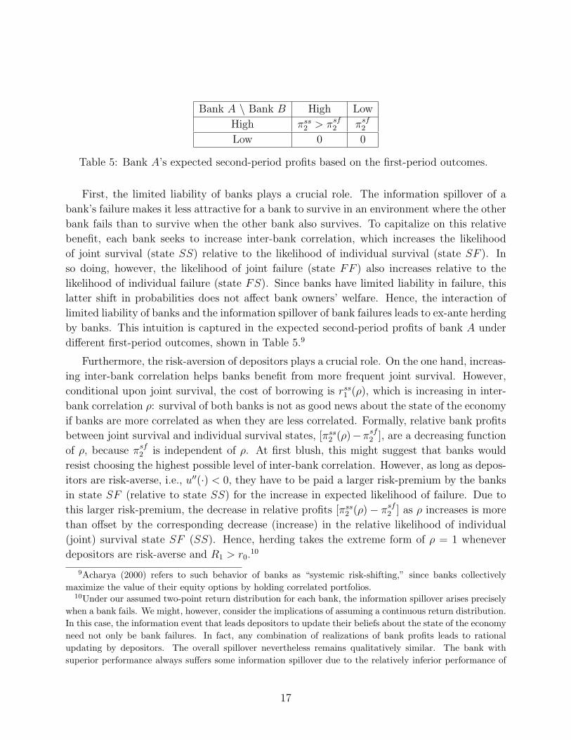
Table 5: Bank A’s expected second-period profits based on the first-period outcomes.

First, the limited liability of banks plays a crucial role. The information spillover of a

bank’s failure makes it less attractive for a bank to survive in an environment where the other

bank fails than to survive when the other bank also survives. To capitalize on this relative

benefit, each bank seeks to increase inter-bank correlation, which increases the likelihood

of joint survival (state SS) relative to the likelihood of individual survival (state SF ). In

so doing, however, the likelihood of joint failure (state FF ) also increases relative to the

likelihood of individual failure (state FS). Since banks have limited liability in failure, this

latter shift in probabilities does not affect bank owners’ welfare. Hence, the interaction of

limited liability of banks and the information spillover of bank failures leads to ex-ante herding

by banks. This intuition is captured in the expected second-period profits of bank A under

different first-period outcomes, shown in Table 5.9

Furthermore, the risk-aversion of depositors plays a crucial role. On the one hand, increas-

ing inter-bank correlation helps banks benefit from more frequent joint survival. However,

conditional upon joint survival, the cost of borrowing is rss1 (ρ), which is increasing in inter-

bank correlation ρ: survival of both banks is not as good news about the state of the economy

if banks are more correlated as when they are less correlated. Formally, relative bank profits

between joint survival and individual survival states, [πss2 (ρ)−πsf

2 ], are a decreasing function

of ρ, because πsf2 is independent of ρ. At first blush, this might suggest that banks would

resist choosing the highest possible level of inter-bank correlation. However, as long as depos-

itors are risk-averse, i.e., u′′(·) < 0, they have to be paid a larger risk-premium by the banks

in state SF (relative to state SS) for the increase in expected likelihood of failure. Due to

this larger risk-premium, the decrease in relative profits [πss2 (ρ)− πsf

2 ] as ρ increases is more

than offset by the corresponding decrease (increase) in the relative likelihood of individual

(joint) survival state SF (SS). Hence, herding takes the extreme form of ρ = 1 whenever

depositors are risk-averse and R1 > r0.10

9Acharya (2000) refers to such behavior of banks as “systemic risk-shifting,” since banks collectivelymaximize the value of their equity options by holding correlated portfolios.

10Under our assumed two-point return distribution for each bank, the information spillover arises preciselywhen a bank fails. We might, however, consider the implications of assuming a continuous return distribution.In this case, the information event that leads depositors to update their beliefs about the state of the economyneed not only be bank failures. In fact, any combination of realizations of bank profits leads to rationalupdating by depositors. The overall spillover nevertheless remains qualitatively similar. The bank withsuperior performance always suffers some information spillover due to the relatively inferior performance of

17

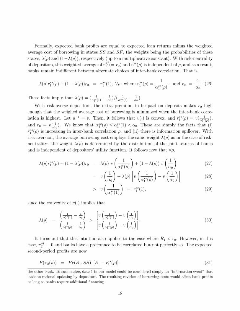
Formally, expected bank profits are equal to expected loan returns minus the weighted

average cost of borrowing in states SS and SF , the weights being the probabilities of these

states, λ(ρ) and (1−λ(ρ)), respectively (up to a multiplicative constant). With risk-neutrality

of depositors, this weighted average of rsf1 (= r0) and rss

1 (ρ) is independent of ρ, and as a result,

banks remain indifferent between alternate choices of inter-bank correlation. That is,

λ(ρ)rss1 (ρ) + (1− λ(ρ))r0 = rss

1 (1), ∀ρ, where rss1 (ρ) =

1

αss1 (ρ)

, and r0 =1

α0

. (26)

These facts imply that λ(ρ) = ( 1αss

1 (1)− 1

α0)/( 1

αss1 (ρ)

− 1α0

).

With risk-averse depositors, the extra premium to be paid on deposits makes r0 high

enough that the weighed average cost of borrowing is minimized when the inter-bank corre-

lation is highest. Let u−1 = v. Then, it follows that v(·) is convex, and rss1 (ρ) = v( 1

αss1 (ρ)

),

and r0 = v( 1α0

). We know that αss1 (ρ) ≤ αss

1 (1) < α0. These are simply the facts that (i)

rss1 (ρ) is increasing in inter-bank correlation ρ, and (ii) there is information spillover. With

risk-aversion, the average borrowing cost employs the same weight λ(ρ) as in the case of risk-

neutrality: the weight λ(ρ) is determined by the distribution of the joint returns of banks

and is independent of depositors’ utility function. It follows now that ∀ρ,

λ(ρ)rss1 (ρ) + (1− λ(ρ))r0 = λ(ρ) v

(1

αss1 (ρ)

)+ (1− λ(ρ)) v

(1

α0

)(27)

= v

(1

α0

)+ λ(ρ)

[v

(1

αss1 (ρ)

)− v

(1

α0

)](28)

> v

(1

αss1 (1)

)= rss

1 (1), (29)

since the convexity of v(·) implies that

λ(ρ) =

(1

αss1 (1)

− 1α0

)(

1αss

1 (ρ)− 1

α0

) >

[v

(1

αss1 (1)

)− v

(1

α0

)][v

(1

αss1 (ρ)

)− v

(1

α0

)] . (30)

It turns out that this intuition also applies to the case where R1 < r0. However, in this

case, πsf2 ≡ 0 and banks have a preference to be correlated but not perfectly so. The expected

second-period profits are now

E(π2(ρ)) = Pr(R1, SS) [R1 − rss1 (ρ)] . (31)

the other bank. To summarize, date 1 in our model could be considered simply an “information event” thatleads to rational updating by depositors. The resulting revision of borrowing costs would affect bank profitsas long as banks require additional financing.

18

On the one hand, by increasing correlation banks increase the probability on SS state relative

to the spillover state SF . However, the cost of borrowing in SS increases too and diminishes

the profits in state SS. Suppose for instance that banks pick ρ such that R1 = rss1 (ρ). This

diminishes profits in state SS to a point where they are zero. If correlation is increased any

further, depositors do not supply funds to banks even in state SS. In anticipation, banks

lower their correlation. Formally, we obtain that for R1 ≤ r0, banks choose a correlation ρ

that is increasing in R1 with ρ = 1 for R1 = r0.

Combining the two cases above, we obtain that there exists R∗1 ≤ r0, a critical level of

second-period promised return R1, such that for all R1 ≥ R∗1, banks choose to be perfectly

correlated. The argument for general case in the proposition with δ > 0 follows along similar

lines once it is recognized that for a given value of R1 (similarly δ), the equilibrium choice of

ρ is a decreasing function of δ (similarly R1). In turn, as long as δ is not too large, banks

choose to be perfectly correlated for all R1 between r0 and a critical threshold R∗∗1 (δ), but

prefer lower levels of inter-bank correlation as R1 rises above this threshold. Intuitively, in the

presence of competition, a given increase in the future profitability of corporate sector leads

to a greater increase in bank profits if they face less competitive margins in lending. This

gives banks an incentive to specialize with respect to other banks in terms of which industries

they lend to. Thus, for a given level of bank competition, banks lend to similar industries

at moderate levels of anticipated profitability of corporate sector, but start differentiating or

specializing if corporate sector prospects improve sufficiently.

In the next section, we show that if depositors of the failed bank choose rationally between

lending to the surviving bank and investing in storage, then herding incentives are further

mitigated when R1 is greater than r0.

5.4 Flight to Quality

Suppose in state SF , the depositors of the failed bank can migrate to the surviving bank.

Clearly, such a migration is individually rational for depositors only if the surviving bank is

viable, that is, if it has profitable opportunities whose returns exceed the promised deposit

rate in some states of the world. We call such migration “flight to quality” since depositors

migrate from a failed bank that had a poor realization of loan returns to a surviving bank

that had better quality of loan performance (and that is also expected to be viable in future).

Empirical evidence supports such migration while also indicating that when information

contagion is sufficiently severe investors flee the banking sector as a whole, taking their

deposits with them.11.

11Saunders and Wilson (1996), for example, examine deposit flows in 163 failed and 229 surviving banksover the Depression era of 1929–1933 in the U.S. They find evidence for flight to quality for years 1929

19

With flight to quality, the surviving bank receives total deposits of two units when it

is the only surviving bank, rather than its previous allocation of one unit. The expected

second-period profits of banks, denoted as E(πFQ2 ), are given as:

E(πFQ2 (ρ)) = E(π2(ρ)) + Pr(R1, SF ) (R1 − r0)

+, (32)

where Pr(R1, SF ) is given by equation (13). The expected profits in the absence of depositor

migration are augmented by the increase in scale of the surviving bank, provided depositors

migrate, that is, if R1 > r0. Thus, when R1 ≤ r0, the equilibrium outcomes with flight to

quality are exactly identical to those under the case analyzed so far.

For R1 > r0, in addition to the competitive effect on margins, there is a disincentive to

herd because of the additional profits in state SF . This can be seen by observing that

∂E(πFQ2 )

∂ρ=

∂E(π2)

∂ρ− (pq + (1− p)(1− q))

dc

dρ(R1 − r0) . (33)

Even in the parameter space where the first term on the right hand side of equation (33) is

positive (as characterized in Proposition 3), the effect of flight to quality through the second

term can weaken the herding incentives.

Proposition 4 (Flight to Quality) Consider δ∗ and the maps R∗1(δ) and R∗∗

1 (δ) as in

Proposition 3. If depositors of a failed bank can migrate to the surviving bank, then ∃ a

map R∗∗∗1 (δ), such that ∀ δ < δ∗, R∗

1(δ) ≤ r0 < R∗∗∗1 (δ) ≤ R∗∗

1 (δ), and

(i) ∀ R1 ∈ [R∗1(δ), R

∗∗∗1 (δ)), banks choose to be perfectly correlated, that is, ρ = 1;

(ii) ∀ R1 ≥ R∗∗∗1 (δ), banks choose correlation ρ < 1 and this correlation decreases in R1.

Furthermore, R∗∗∗1 (δ) →∞ as δ → 0, and R∗∗∗

1 (δ) is decreasing in δ.

We interpret Propositions 3 and 4 as the “procyclicality” of bank herding incentives.

5.5 Procyclicality of Herding

Historical evidence on bank lending and its fluctuations suggests that the level of aggregate

bank lending is pro-cyclical. The present analysis suggests however that even the industry

and 1933: withdrawals from the failed banks during these years were associated with deposit increases insurviving banks. However, for the period 1930–1932, deposits in failed banks as well as surviving banksdecreased, which the authors interpret as evidence for contagion. Importantly, the deposit decrease in thefailed banks exceeded those at the surviving banks, most likely a manifestation of rational updating of beliefsabout bank prospects by informed depositors. In another study, Saunders (1987) studies the effects on theother banks’ deposits due to two announcements regarding an individual bank in April and May 1984. Whilethe first announcement did not have a significant effect, the second one, made by the U.S. Office of theComptroller of the Currency, resulted in a flight to quality.

20

concentration of aggregate bank lending should exhibit a procyclical pattern: lending to

some industry surges in the economy at peaks in the cycle affecting that industry, and a

sharp contraction ensues at troughs of the cycle.

At business cycle peaks, the expected future return on bank investments (R1) is lower, for

example, due to a possible slow-down in the economy. Thus, the expected benefit to banks

in differentiating from other banks is not large. Simply stated, there is not much business for

banks in the forthcoming periods. Such an economic state causes herding incentives to dom-

inate and banks continue to lend to a common industry. This is more likely if bank margins

are unlikely to be affected significantly by competition in lending to a common industry. This

suggests that banking sectors that are highly concentrated should be more prone to herding.

In a similar vein, all else being equal, an industry with a greater concentration of banks is

likely to be the industry banks herd on. Finally, if an industry experiences a technology shock

whereby the demand for bank funds in the industry rises steeply, then banks are more likely

to herd on such an industry: as demand is high, bank margins do not get eroded quickly

upon herding in this industry.

In contrast, at business-cycle troughs, the future profits from bank investments are at-

tractive (higher R1). The consequent expected benefit of survival when other banks fail, for

example, through an increase in the scale of business, mitigate herding and in fact can be

sufficient to overcome the benefits of herding. The result is that banks differentiate at the

troughs, lending to a common industry is retrenched, and greater reallocation of bank credit

across industries takes place. Furthermore, if returns on bank investments indeed exhibit

such cyclical behavior, then aggregate bank lending to a particular industry must show a

“trend-chasing” behavior. Specifically, at business cycle peaks, past returns are high, above

the long-term trend, and conditionally expected to fall, whereas at business cycle troughs,

past returns are low, below the long-term trend, and conditionally expected to rise.

Indeed, Mei and Saunders (1997) demonstrate that investments in real-estate by U.S. fi-

nancial institutions have tended to be greater precisely in those times when the real-estate

sector looked less attractive from an ex-ante standpoint. The ex-ante predictor of real-estate

sector outlook is constructed using the historical returns on traded real-estate investment

trusts (REITs) and exhibits a mean-reverting cyclical pattern. In more recent evidence, Hog-

garth and Pain (2002) document that the growth in bank loans to real estate and construction

sectors in the United Kingdom rose disproportionately in the boom period of the economy:

in the period December 1987 to December 1989, lending to these sectors grew by 55% and

40% respectively, compared to around 25% for other sectors. Finally, the plot of industry

concentration of bank loans in Massachussets in the United States during the period 1986–

1996 (Figure 2) shows an increase in concentration upto 1991 (the trough of the recession),

being driven primarily by lending to the real-estate sector, and a decrease in concentration

afterwards.

21

Interpreting such behavior at the level of an individual bank may suggest a behavioral

inefficiency on part of the loan officers: banks appear to increase their lending to an industry

when its expected returns are falling and reduce their lending when its expected returns are

rising. However, when viewed in the context of the herding incentives of banks, this is ex-

actly the lending behavior one should anticipate from profit-maximizing banks. Behavioral

explanations such as the “institutional memory loss” in Berger and Udell (2002) are poten-

tially consistent with the level of aggregate bank lending being procyclical but it is less clear

that these explanations imply a procyclical variation also in the industry concentration of

aggregate bank lending. We find the evidence of Mei and Saunders (1997) and Hoggarth

and Pain (2002) supportive of our analysis since they examine industry-level lending which

relates more directly to correlated lending and its procyclicality.

Furthermore, if bank lending is driven by herding incentives during economic booms and

by competitive incentives during economic downturns, then there should be greater cancel-

lation of existing credit and its replacement with new credit during downturns than during

booms. Dell’Ariccia and Garibaldi (2003)’s results confirm this. They find that excess credit

reallocation in the United States during the period 1979 to 1999, measured as the sum of gross

credit flows in excess of net changes in the aggregate level of credit, is countercylical: excess

credit reallocation is negatively correlated to the U.S. GDP fluctuations. While such credit

reshuffling may arise simply from banks cutting loans to unsuccessful sectors and reallocating

credit to profitable ones, their evidence shows that the reallocation is most countercyclical

for real-estate lending. Jointly with the evidence of Mei and Saunders (1997), this provides

support for our theory that banks have incentives to herd on a given sector, say real-estate,

during booms and to differentiate by lending to different sectors during downturns.

Unfortunately, comprehensive empirical documentation on asset correlations of banks is

sparse. In a recent study, Nicolo and Kwast (2001) find that the creation of large and

complex banking organizations increases the extent of diversification at the individual bank

level and decreases the individual bank’s risk. However, they document that this leads to

a greater correlation of bank stock returns. Specifically, they find that stock prices of the

biggest 22 U.S. banking organizations tended to increasingly move in lockstep during 1989–

1999. The degree of correlation in stock price movements increased from 0.41 in 1989 to

0.56 during 1996–1999. They suggest on basis of this evidence that “Troubles at a single

bank could easily generate investor perceptions of similar troubles at other big banks.” More

direct documentation of the correlations in loan portfolios of banks is necessary to provide

additional evidence about the extent of herding in a banking sector and its procyclicality.

It is reasonable to expect other parameters of our model to also vary over the business

cycle. For example, at business cycle peaks, the likelihood of being in a bad state of the

economy in future may be higher. Numerical examples, available upon request from the

authors, illustrate that herding is stronger (in terms of the range of values of R1 for which

22

banks choose high inter-bank correlation) when the likelihood of bad state of the economy

is high (p low) and when the systematic risk of loans is high (q high). These results further

strengthen our interpretation of Proposition 4 as procyclicality of herding.

6 Inefficiency of Herding

When banks herd, they may bypass lending to more profitable firms and industries. To

embed the inefficiency that arises from this effect, we consider the choice of bank investments

as being between two uncorrelated industries. If banks choose to lend to the same industry,

then they are perfectly correlated (ρ = 1), and if they lend to different industries, then they

are uncorrelated (ρ = 0).

For simplicity, we assume that both industries are identical and both have the same

expected production technology f(x), where x is the total amount of lending to the industry.

There are diminishing returns to scale so that f ′(x) > 0 but f ′′(x) < 0. Each firm in the

industry is assumed to be infinitesimally small but perfectly correlated to all other firms in

that industry. That is, all firms in an industry are perfectly correlated but differ in expected

returns. Furthermore, all firms in the economy have the same likelihood of success and failure.

In the analysis so far, θ(ρ)Rt represented the return banks could charge on loans to their

borrowers. Consider, for example, the first period (t = 0). Now suppose we can write

θ(0) = 1, α0R0 = γf ′(1), and α0θ(1)R0 = f ′(2) where 1 < γ < f ′(0)f ′(1)

. Note that α0 is

the likelihood of high return on bank loans in the first period. Thus, when banks lend to

the same industry (a total of two units of lending to that industry), competition erodes the

risk-adjusted return they can charge on loans and it is simply the marginal expected rate of

production in the industry (f ′(2)). However, when banks lend to different industries (a total

of one unit of lending to each industry), each bank can earn a greater risk-adjusted return

that lies between f ′(0) and f ′(1).

Given the diminishing returns to scale, f(2) < 2f(1), and the expected output generated

by the corporate sector is maximized when banks invest in different industries. Therefore,

from a production efficiency standpoint, the socially optimal level of inter-bank correlation

is ρ = 0. However, as we have shown, because of the information spillover, banks in general

choose a higher level of correlation. This is socially inefficient: Banks overinvest in some

industries to maximize their private interests, and, in the process, bypass superior projects

in other industries.

23

7 Effect of Heterogeneity and More Than Two Banks

We extend the basic model to derive additional conclusions regarding properties of banks for

which information contagion and herding incentives are likely to be stronger.

Suppose there are three banks in the model, but one of the banks is a “foreign” bank. The

foreign bank also has access to a set of depositors with a unit of consumption good each period.

The foreign bank is affected by a foreign systematic risk factor, whereas the two “domestic”

banks are affected by the same domestic systematic risk factor. One interpretation of this

setting is that the foreign bank is collecting deposits in a country but its nature of business

differs fundamentally from that of domestic banks of that country (for example, retail vs. high

net–worth lending). Another interpretation is that the foreign bank has a greater proportion

of loan portfolio in its own country, whereas domestic banks are localized to just their own

country for both borrowing and lending. That is, the words “foreign” and “domestic” can

be metaphors for some richer heterogeneity amongst banks due to specialization in lending.

For simplicity, we take these interpretations to the extreme and assume that domestic and

foreign banks are affected by essentially different factors. Our results are robust to allowing

for some commonality across factors.

Suppose that the probabilities of the good state and the high return have the same value

ex-ante for all banks, the return realizations are drawn from the same distribution for the two

domestic banks, but they are drawn from an independent distribution for the foreign bank.

Under this structure, the realization of domestic banks’ returns conveys no information about

the foreign systematic risk factor, and vice versa. The information spillover for domestic banks

arises only from each other’s performance. The updating by depositors and the promised

rates are also the same for the two domestic banks and identical to the values derived in the

analysis thus far. For the foreign bank, the situation is similar to the case where there is

no information spillover. Formally, the probability of a high return for the foreign bank in

the second period, given the foreign bank had a high return in the first period, is simply αs1

(equation 10). In turn, the promised return to the foreign bank’s depositors at date 1, is

simply rs1, where from Proposition 2, rs

1 < rsf1 . Therefore, when one of the domestic banks

fails, the foreign bank (if it has survived) can attract depositors by offering a lower promised

rate than the surviving domestic bank.

More generally, upon the failure of some banks, deposits rationally “fly” to banks that

are considered different from the failed banks, and in turn, are deemed relatively safe. Banks

considered to be similar to the failed ones observe a decrease in their deposit base (possibly

even a run). Calling this phenomenon as “flight to quality” is even more appropriate than

before since depositors migrate to a set of banks deemed safer than the banks they had lent to

earlier. To summarize, the benefit from such flight to quality to dissimilar banks accentuates

24

the information spillover (contagion) for similar banks.12

We conclude that information spillover is more likely to arise from the failure of banks

whose portfolio returns are anticipated to be more correlated with the overall state of economy.

Furthermore, the information spillover is likely to be localized, affecting those banks the most

whose portfolio returns are also anticipated to be highly correlated with the overall economy.

By implication, herding amongst banks should be a localized phenomenon as well. Finally,

the lack of relative expertise of “foreign” banks in lending to “domestic” industries should

further weaken their incentives to herd with “domestic” banks.

8 Discussion

8.1 Relationship to Reputational Herding

In the literature on herding (surveyed in Devenow and Welch 1996), herding is often an

outcome of sequential decisions, with the decision of one agent conveying information about

some underlying economic variable to the next set of decision-makers. In Scharfstein and Stein

(1990) model, for example, herding behavior is driven by managerial concerns for reputation

and involves sequential investments. Herding, however, need not always be the outcome of

such an informational cascade. It can also arise from a coordination game. In our paper,

herding is a simultaneous ex-ante decision of banks to coordinate correlated investments. In

this sense, our paper is closest to Rajan (1994) who also models coordination by “short-

termist” bank managers in announcing losses on loan portfolios and adjusting credit policies.

In Rajan’s model, it is privately optimal for managers to fail when other managers fail so

as to “share the blame,” and this gives incentives for correlated announcements of losses. In

contrast, in our model, banks have leverage and given limited liability, it is privately optimal

for bank owners to succeed when other banks succeed: each bank’s success subsidizes the

other banks’ borrowing costs. These two mechanisms are complementary to each other.

Next, we identify some key differences between their implications.

In the reputation-based herding literature, alignment of managerial objective with firm

12Consistent with this, Kaufman’s (1994) survey on systemic risk documented abnormal negative returnsof other banks when a given bank fails, only if the surviving banks also invested in the same product ormarket area. In another piece of supporting evidence, Schumacher (2000) examined the 1995 banking crisisin Argentina triggered by the 1994 Mexican devaluation. Her analysis showed evidence of bank-specificcontagion and flight to quality, rather than a contagion to the whole system. More specifically, after thefailure of some domestic wholesale banks, surviving domestic wholesale banks suffered significant depositlosses. The suspension of retail bank operations increased the withdrawals from surviving small retail banks.But the foreign retail banks, and to some extent large domestic banks, had significant increases in theirdeposits during the crisis.

25

profits acts as a countervailing force to herding behavior. For example, Rajan adds profits

to the objective function of managers and demonstrates this effect over a set of parameters.

This suggests that bank herding should decrease in the extent of managerial (or central

loan officers’) alignment with bank profits, proxied say by their incentive compensation.

In our paper, managers of limited-liability banks maximize bank profits, and yet there is

herding. Aligning managerial objectives with maximization of bank profits may thus not be

sufficient to ameliorate herding behavior. Put even more strongly, maximization of profits

may not be a countervailing force to herding behavior at all. Herding may thus be a robust

economic outcome, even under settings where managerial discretion over timing of charge-

offs is restricted, and more generally, where managerial agency problems are absent. While

we are not aware of a test linking herding behavior to incentive compensation, our theory

in contrast to Rajan’s, would predict that bank herding in fact increases in the extent of

managerial alignment with bank profits.

In both Scharfstein and Stein (1990) and Rajan (1994), a low return on investment in the

bad state is more likely than a high return on investment in the good state: There is only

one way for managers to be correct (more likely in the good state), but several different ways

for them to be incorrect (more likely in the bad state). This is the main factor driving the

herding results in these papers. In contrast, we assume a symmetric distribution: In Table 1,

the conditional probability q does not depend on whether the state is Good or Bad. In spite

of this assumption, an asymmetry arises in the payoffs of bank owners due to the interaction

of limited liability and information spillover. It can be shown that an asymmetric distribution

of outcomes in our model (that is, q in Good state being smaller than q in Bad state) makes

the information spillover more severe and strengthens the herding incentives. These results

are available from authors upon request.

Finally, a relevant factor for the managerial herding theory is the reward to managers for

relative ability, that is, the reward for being successful when others fail. The papers in this

literature typically do not model such relative rewards, but instead argue qualitatively that

they counteract herding incentives. Modeling of relative rewards such as superior lending

margins from specialization and “flight to quality” are novel features of our analysis that give

rise to the procyclical herding pattern.

8.2 Inter-Bank Linkages

Rochet and Tirole (1996), Allen and Gale (2000), and Dasgupta (2000), to cite a few, consider

contagion arising from inter-bank linkages such as inter-bank deposits that provide liquidity

insurance to banks. As such, the precise mechanism through which contagion or spillover

take place do not affect the main thrust of our herding results. However, a series of recent

26

empirical papers13, suggest that the inter-bank linkage channel may not have as much “bite”

as the theoretical literature has assumed so far. These studies estimate the matrix of bilateral

exposures among banks and do not find significant potential for failures resulting from inter-

bank linkages. In addition, Elsinger, Lehar and Summer (2003) show that among the sources

of systemic risk the direct effects from correlated exposures of banks are far more important

than contagion effects. They conclude that “[The] preoccupation with domino effects should

not distract regulators from the most important source of systemic risk: the correlation

structure in the banks’ asset portfolios”. Our paper is an attempt towards understanding the

factors that affect banks’ choice of correlation between their asset portfolios.

8.3 Information Disclosure

The release of bank-specific information can mitigate information contagion, since depositors

would know the realization of systematic and idiosyncratic shocks in causing the bank failures.

Gorton (1985), Gorton and Mullineaux (1987), and Park (1991) discuss how the spreading

of banking panics was prevented by the disclosure of bank-specific information in the 19th

century in the United States. One of the methods used was a selective closure of banks. This

revealed the information that the banks that were let to continue operation were healthy. This

restored confidence and prevented contagion, the spreading of the panic to healthy banks.

Our analysis yields the novel prediction that by reducing the likelihood of contagion, such

information disclosure should also reduce the ex-ante herding incentives of banks and add

further systemic stability to the banking sector.

8.4 Deposit Insurance

Most banking systems have deposit insurance and a requirement that banks pay some in-

surance premia. Full deposit insurance renders deposit rates insensitive to fluctuations in

bank’s health and reduces information spillover of the sort we described. However, the pro-

vision of deposit insurance is only partial in most countries. Furthermore, banks also have

subordinated debt in their capital structures that is typically not insured and is often the

marginal source of funds. Interest rates on both uninsured deposits and subordinated debt

should respond to information pertaining to the bank’s health. Thus, in a world with de-

posit insurance, information spillover would still arise, but its effect on bank profits would

be restricted to the amount of uninsured bank debt. To this extent, deposit insurance only

partially mitigates ex-post information spillover, and in turn, ex-ante herding. Furthermore,

any analysis of deposit insurance must account for an important cost: the lack of incentives

13For example, Sheldon and Maurer (1998) for Switzerland, Furfine (1999) for the United States, Upperand Worms (2000) for Germany, and Wells (2002) for the United Kingdom.

27

for insured depositors to differentiate between sound and unsound banks which reduces the

competitive (flight to quality) benefits to banks.

Herding by banks can also impose excessive costs on the deposit insurer as the likelihood of

joint failures increases. As long as the deposit insurance premia are based only on individual

bank characteristics and not on inter-bank correlations (as is currently the practice), the

premia are unlikely to make banks internalize completely the costs that herding imposes on

the insurer.

9 Conclusion

While most studies of systemic risk and financial fragility are concerned with the ex-post

effects of bank failures, our paper demonstrates that analyzing the ex-ante response of banks

to these effects is important. The extent of herding can be considered the ex-ante aspect

of systemic risk: It affects the likelihood of joint failure of banks, but also affects and is

affected by the extent of information contagion, which can be considered the ex-post aspect

of systemic risk. An important implication of our unified analysis is the pro-cyclical nature

of herding amongst banks, and it conforms well with empirical evidence. Our analysis also

highlights the need for a more complete empirical analysis of the reciprocal causality between

inter-bank correlations and information contagion.

Finally, an important issue for future research appears to be the integration of regulatory

closure policies in frameworks such as ours. Extant empirical evidence suggests that regu-

latory actions taken in response to banking problems vary significantly. In many episodes,

regulatory actions depend on whether the problems arise from idiosyncratic reasons specific

to particular institutions or from potential threats to the whole system (Santomero and Hoff-

man 1999). In addition, Kasa and Spiegel (2003) show that regulators cannot commit to be

tough when the crisis is systemic. This leads to a “too-many-to-fail” guarantee where banks

rationally anticipate a greater likelihood of bail out if they fail together. As demonstrated in

Acharya (2000), this generates a collective moral hazard where banks herd to extract greater

regulatory forbearance. The contribution of regulatory guarantees to the observed levels of

inter-bank correlations requires further theoretical and empirical investigation.

28

A Proofs

While in the text we use ρ as the measure of correlation, for simplicity we use the parameter

c in our proofs, where ρ and c are related by equation (3). Since ∂ρ∂c

> 0, this does not affect

any of our results. Recall that c ∈ [cmin = q2, cmax = q], and correspondingly, ρ ∈ [0, 1].

The following lemmas are employed towards proving the main propositions of the paper.

Lemma A.1 The probability of a high return, given that both banks had high returns from

their first investments, is decreasing in c. Formally,∂αss

1

∂c< 0, ∀ p, q. In turn, the cost of

borrowing is increasing in c, i.e.,∂rss

1

∂c> 0, ∀ p, q.

Proof: From equation (17), we obtain

∂αss1

∂c=

[pq + (1− p)(1− q)] [(1− 2q)(1− p) + c]− [pcq + (1− p)(1− q)(1− 2q + c)]

[(1− 2q)(1− p) + c]2(34)

which is negative, since the numerator equals −p(1 − p)(2q − 1)2, which is always less than

zero. From equation (18) for rss1 and the fact that u′(·) > 0, it follows that

∂rss1

∂c> 0. ♦

Lemma A.2 When banks are perfectly correlated, the probability of a high return, given that

both banks had high returns from their first investments, is greater than the prior probability

of a high return. Formally, αss1 (cmax) > α0, ∀ p, q.

Proof: From equations (4) and (17), the claim reduces to showing that

αss1 (cmax) =

pq2 + (1− p)(1− q)2

pq + (1− p)(1− q)= αs

1 > α0 = pq + (1− p)(1− q). (35)

This holds since pq2 + (1− p)(1− q)2 − [pq + (1− p)(1− q)]2 = p(1− p)(2q − 1)2 > 0. Also

note that αss1 (cmax) = αs

1. Therefore, rss1 (cmax) = rs

1. ♦

These lemmas and the maintained assumption that u′(·) > 0 imply the following result.

Lemma A.3 ∀ p, q, and c, αss1 (c) > α0 and rss

1 (c) < r0.

Proof of Proposition 2: The proposition is a direct consequence of Lemmas A.1–A.3. ♦

Proof of Proposition 3: We need to consider two cases as discussed in Section 5.3. To

perform analysis in the variable c, let θ(c) = 1 − δρ(c). We will first prove the case where

R1 ≥ r0. To start with, assume that θ(c) = 1 for all c, that is, δ = 0.

29

If R1 ≥ r0, then from equation (24), the expected second-period profits are

E(π2(c)) =[pq2 + (1− p)(1− q)2

][R1 − (λ(c)rss

1 (c) + (1− λ(c))r0)]. (36)

We wish to show that

∂E(π2(c))

∂c= −

[pq2 + (1− p)(1− q)2

] [∂λ(c)

∂c(rss

1 (c)− r0) + λ(c)∂rss

1 (c)

∂c

](37)

is greater than zero. Since [pq2 + (1− p)(1− q)2] > 0, the sign of the expression above is

determined by the sign of the expression inside the second set of square brackets on the right

hand side of equation (37). We prove this in steps:

(i) From the expression for λ(c) in equation (25), it follows that

∂λ(c)

∂c=

pq + (1− p)(1− q)

pq2 + (1− p)(1− q)2. (38)

(ii) From equations (17) and (18), it follows that

u(rss1 (c)) =

(1− 2q)(1− p) + c

pcq + (1− p)(1− q)(1− 2q + c). (39)

Taking the partial derivative of both sides with respect to c, we get

u′(·)∂rss1 (c)

∂c=

[pcq + (1− p)(1− q)(1− 2q + c)]− [(1− 2q)(1− p) + c] [pq + (1− p)(1− q)]

[pcq + (1− p)(1− q)(1− 2q + c)]2

=p(1− p)(1− 2q)2

[pcq + (1− p)(1− q)(1− 2q + c)]2. (40)

Therefore, we obtain that

λ(c)∂rss

1 (c)

∂c=

1

u′(rss1 (c))

p(1− p)(1− 2q)2

[pq2 + (1− p)(1− q)2] [pcq + (1− p)(1− q)(1− 2q + c)](41)

(iii) Finally, from equations (4), (17) and (25), we obtain

∂λ(c)

∂c(rss

1 (c)− r0) =pq + (1− p)(1− q)

pq2 + (1− p)(1− q)2

[u−1

(1

αss1

)− u−1

(1

α0

)], (42)

where for simplicity we have suppressed the dependence of αss1 on c. Let v = u−1. Since u(·)

is increasing and concave, v′(·) > 0 and v′′(·) > 0. Thus,[v

(1

αss1

)− v

(1

α0

)]< v′

(1

αss1

) (1

αss1

− 1

α0

). (43)

30

Substituting for α0 and αss1 from equations (4) and (17),

v′(

1

αss1

) (1

αss1

− 1

α0

)=

1

u′(rss1 (c))

[(1− 2q)(1− p) + c

pcq + (1− p)(1− q)(1− 2q + c)− 1

pq + (1− p)(1− q)

]= − 1

u′(rss1 (c))

{p(1− p)(1− 2q)2

[pcq + (1− p)(1− q)(1− 2q + c)] [pq + (1− p)(1− q)]

}.

Therefore,

∂λ(c)

∂c(rss

1 (c)− r0) < − 1

u′(rss1 (c))

1

(pq2 + (1− p)(1− q)2)

[p(1− p)(1− 2q)2

pcq + (1− p)(1− q)(1− 2q + c)

]< −λ(c)

∂rss1 (c)

∂c. (44)

Using steps (i), (ii) and (iii) above, it follows that

∂λ(c)

∂c(rss

1 (c)− r0) + λ(c)∂rss

1 (c)

∂c< 0. (45)

Thus, if R1 ≥ r0 and δ = 0, then E(π2(c)) is increasing in c, and banks pick the highest

possible inter-bank correlation c = cmax, that is ρ = 1.

Now we look at the general case where θ(c) = 1− δρ(c), and δ > 0.

Banks choose the level of correlation to maximize the total expected profits:

maxc∈[q2,q]

Pr(R0) [θ(c)R0 − r0] + Pr(R1, SS) [θ(c)R1 − rss1 (c)] + Pr(R1, SF ) [R1 − rsf

1 ].

Denoting the total expected profits as Π, we can rewrite them as

Pr(R0) [R0 − r0] + Pr(R1, SS) [R1 − rss1 (c)] + Pr(R1, SF ) [R1 − rsf

1 ]︸ ︷︷ ︸Expected profits without competition = Π(δ=0)

+

Pr(R0) [(θ(c)− 1)R0] + Pr(R1, SS) [(θ(c)− 1)R1].

To maximize the expected profits we look at the first-order condition:

∂

∂c[Π(δ = 0)] +

{θ′(c) [Pr(R0)R0 + Pr(R1, SS)R1] +

∂ Pr(R1, SS)

∂c[(θ(c)− 1)R1]

}= 0.

That is, the first-order condition is

∂

∂c[Π(δ = 0)]︸ ︷︷ ︸

>0

− δ∂ρ

∂c

[Pr(R0)R0 + Pr(R1, SS)R1]︸ ︷︷ ︸>0

+∂ Pr(R1, SS)

∂c︸ ︷︷ ︸>0

R1

= 0. (46)

31

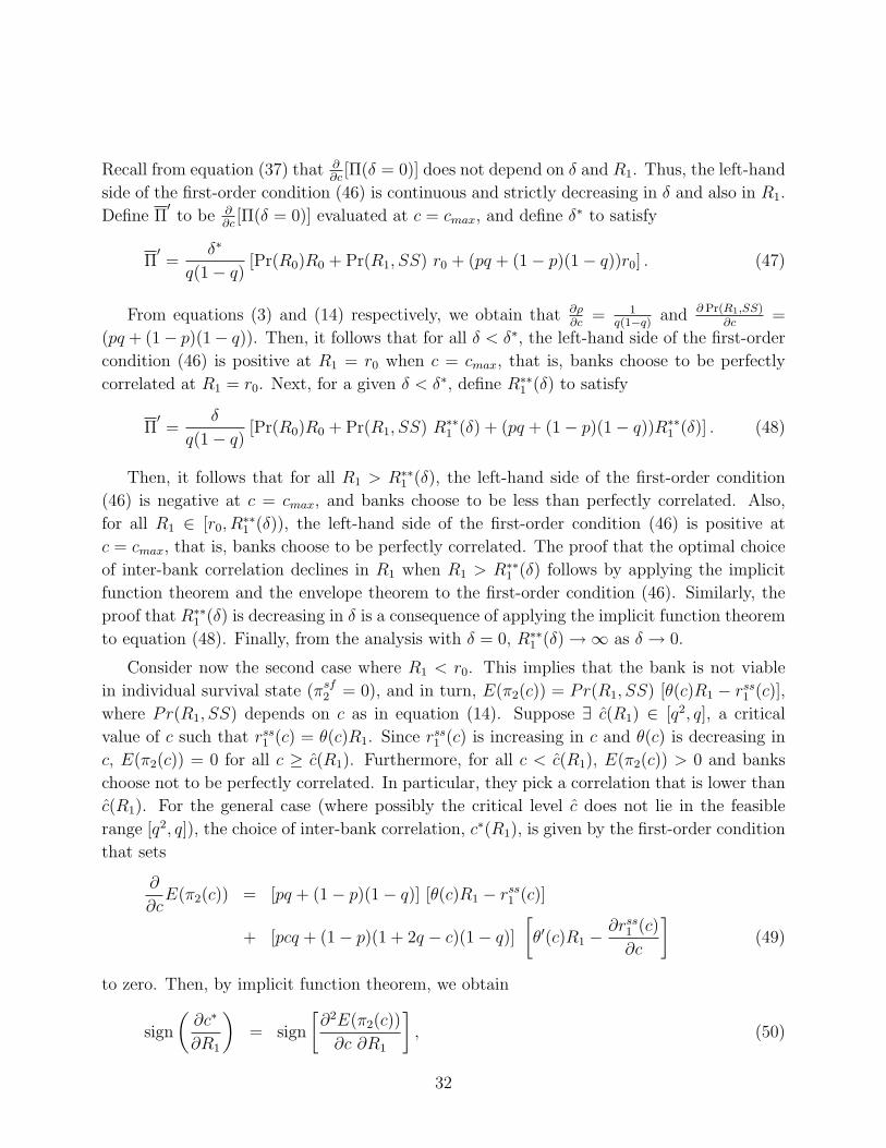
Recall from equation (37) that ∂∂c

[Π(δ = 0)] does not depend on δ and R1. Thus, the left-hand

side of the first-order condition (46) is continuous and strictly decreasing in δ and also in R1.

Define Π′to be ∂

∂c[Π(δ = 0)] evaluated at c = cmax, and define δ∗ to satisfy

Π′=

δ∗

q(1− q)[Pr(R0)R0 + Pr(R1, SS) r0 + (pq + (1− p)(1− q))r0] . (47)

From equations (3) and (14) respectively, we obtain that ∂ρ∂c

= 1q(1−q)

and ∂ Pr(R1,SS)∂c

=

(pq + (1− p)(1− q)). Then, it follows that for all δ < δ∗, the left-hand side of the first-order

condition (46) is positive at R1 = r0 when c = cmax, that is, banks choose to be perfectly

correlated at R1 = r0. Next, for a given δ < δ∗, define R∗∗1 (δ) to satisfy

Π′=

δ

q(1− q)[Pr(R0)R0 + Pr(R1, SS) R∗∗

1 (δ) + (pq + (1− p)(1− q))R∗∗1 (δ)] . (48)

Then, it follows that for all R1 > R∗∗1 (δ), the left-hand side of the first-order condition

(46) is negative at c = cmax, and banks choose to be less than perfectly correlated. Also,

for all R1 ∈ [r0, R∗∗1 (δ)), the left-hand side of the first-order condition (46) is positive at

c = cmax, that is, banks choose to be perfectly correlated. The proof that the optimal choice

of inter-bank correlation declines in R1 when R1 > R∗∗1 (δ) follows by applying the implicit

function theorem and the envelope theorem to the first-order condition (46). Similarly, the

proof that R∗∗1 (δ) is decreasing in δ is a consequence of applying the implicit function theorem

to equation (48). Finally, from the analysis with δ = 0, R∗∗1 (δ) →∞ as δ → 0.

Consider now the second case where R1 < r0. This implies that the bank is not viable

in individual survival state (πsf2 = 0), and in turn, E(π2(c)) = Pr(R1, SS) [θ(c)R1 − rss

1 (c)],

where Pr(R1, SS) depends on c as in equation (14). Suppose ∃ c(R1) ∈ [q2, q], a critical

value of c such that rss1 (c) = θ(c)R1. Since rss

1 (c) is increasing in c and θ(c) is decreasing in

c, E(π2(c)) = 0 for all c ≥ c(R1). Furthermore, for all c < c(R1), E(π2(c)) > 0 and banks

choose not to be perfectly correlated. In particular, they pick a correlation that is lower than

c(R1). For the general case (where possibly the critical level c does not lie in the feasible

range [q2, q]), the choice of inter-bank correlation, c∗(R1), is given by the first-order condition

that sets

∂

∂cE(π2(c)) = [pq + (1− p)(1− q)] [θ(c)R1 − rss

1 (c)]

+ [pcq + (1− p)(1 + 2q − c)(1− q)]

[θ′(c)R1 −

∂rss1 (c)

∂c

](49)

to zero. Then, by implicit function theorem, we obtain

sign

(∂c∗

∂R1

)= sign

[∂2E(π2(c))

∂c ∂R1

], (50)

32

where

∂2E(π2(c))

∂c ∂R1

= [pq + (1− p)(1− q)]θ(c) + [pcq + (1− p)(1 + 2q − c)(1− q)]θ′(c). (51)

It follows now that if θ(c) = 1− δρ(c), so that θ′(c) = − δq(1−q)

, then there is a critical level

of δ below which c∗(R1) is increasing in R1. Since c∗(r0) = cmax whenever δ is sufficiently

small (from the proof for the first case), it follows that it is possible to identify δ∗ and maps

R∗1(δ) ≤ r0 < R∗∗

1 (δ) such that the statement in the proposition holds. ♦

Proof of Proposition 4: For R1 ≤ r0, E(πFQ2 ) is identical to E(π2), and analysis in the

proof of Proposition 3 for this range of R1 applies. For R1 > r0, E(πFQ2 ) and E(π2) diverge

due to the profits in state SF (or FS) from flight-to-quality. Now, the first-order condition

for the choice of inter-bank correlation (from equation 33) is

∂E(πFQ2 )

∂c=

∂E(π2)

∂c− (pq + (1− p)(1− q)) (R1 − r0) . (52)

That is, the first-order condition with flight-to-quality is identical to equation (46), except

that the term [−(pq + (1− p)(1− q))(R1− r0)] must be added to the left-hand side. The rest

of the proof follows closely along the lines of Proposition 3. In particular, R∗∗∗1 (δ) satisfies

Π′

=δ

q(1− q)[Pr(R0)R0 + Pr(R1, SS) R∗∗∗

1 (δ) + (pq + (1− p)(1− q))R∗∗∗1 (δ)]

+ (pq + (1− p)(1− q)) [R∗∗∗1 (δ)− r0] , (53)

so that R∗∗∗1 (δ) < R∗∗

1 (δ). The rest of the details are omitted for sake of brevity. ♦

33

References

[1] Acharya, V. (2000) “A Theory of Systemic Risk and Design of Prudential Bank Regulation,”Working Paper, London Business School.

[2] Aharony, J. and I. Swary (1983) “Contagion Effects of Bank Failures: Evidence from CapitalMarkets,” Journal of Business, 56(3), 305-317.

[3] Allen, F. and D. Gale (2000) “Financial Contagion,” Journal of Political Economy, 108, 1–33.

[4] Berger, A. and G. Udell (2002) “The Institutional Memory Hypothesis and the Procyclicality ofBank Lending Behavior,” Working Paper, Board of Governors of the Federal Reserve System,Washington, DC.

[5] Borio, C., Furfine, C. and P. Lowe (2001) “Procyclicality of the Financial System and FinancialStability: Issues and Policy Options,” Working Paper, Bank for International Settlements.

[6] Calomiris, C. and G. Gorton (1991) “The Origins of Banking Panics: Models, Facts, and BankRegulation,” in R. Glenn Hubbard (ed.), Financial Markets and Financial Crises, University ofChicago Press, 109–173.

[7] Calomiris, C. and J. Mason (1997) “Contagion and Bank Failures During the Great Depression:The June 1932 Chicago Banking Panic,” American Economic Review, 87(5), 863-883.

[8] Calomiris, C. and J. Mason (2000) “Causes of U.S. Bank Distress During the Depression,”NBER Working Paper #7919, Cambridge, MA, USA.

[9] Carron, A. (1982) “Financial Crises: Recent Experience in U.S. and International Markets,”Brookings Papers on Economic Activity, no:2, 395-418.

[10] Chari, V. and R. Jagannathan (1988) “Banking Panics, Information, And Rational Expecta-tions Equilibrium,” Journal of Finance, 43-3, 749-761.

[11] Chen, Y. (1999) “Banking Panics: The Role of the First-Come, First-Served Rule and Infor-mation Externalities,” Journal of Political Economy, 107(5), 946–968.

[12] Cooperman, E., Lee, W. and G. Wolfe (1992) “The 1985 Ohio Thrift Crisis, the FSLIC’sSolvency and Rate Contagion for Retail CDs,” Journal of Finance, 47(3), 919-941.

[13] Cornell, B. and A. Shapiro (1986) “The Reaction of Bank Stock Prices to the InternationalDebt Crisis,” Journal of Banking and Finance, 10, 55-73.

[14] Dasgupta, A. (2000) “Financial Contagion through Capital Connections: A Model of the Originand Spread of Banking Panics,” Working Paper, London School of Economics.

[15] Dell’Ariccia, G. and P. Garibaldi (2003) “Gross Credit Flows,” Working Paper, InternationalMonetary Fund, Washington, D.C.

34

[16] Devenow, A. and I. Welch (1996) “Rational Herding in Financial Economics,” Working Paper,Anderson School of Management, UCLA.

[17] Diamond, D. and P. Dybvig (1983) “Bank Runs, Deposit Insurance, And Liquidity,” Journalof Political Economy, 91-3, 401-419.

[18] Docking, D., Hirschey, M. and E. Jones (1997) “Information and Contagion Effectsof BankLoan-loss Reserve Announcements,” Journal of Financial Economics, 43(2), 219-240.

[19] Elsinger H., A. Lehar and M. Summer (2003) “Risk Assesment of Banking Systems,” mimeo.,University of Vienna.

[20] Furfine, C.H. (1999) “Interbank Exposures: Quantifying the Risk of Contagion,” BIS WorkingPaper, no:70, Basel.

[21] Gay, G., Timme, S. and K. Yung (1991) “Bank Failure and Contagion Effects: Evidence fromHong Kong,” Journal of Financial Services Research, 14(2), 153-165.

[22] Gorton, G. (1985) “Clearinghouses and the Origin of Central Banking in the United States,”The Journal of Economic History, 42, 277–284.

[23] Gorton, G. (1988) “Banking Panics and Business Cycles,” Oxford Economic Papers, 40,751-781.

[24] Gorton, G. and D. Mullineaux (1987) “The Joint Production of Confidence: Endogenous Reg-ulation and Nineteenth Century Commercial-Bank Clearinghouses,” Journal of Money, Credit,and Banking, 19, 457–467.

[25] Hasan, I. and G. Dwyer (1994) “Bank Runs in the Free Banking Period,” Journal of Money,Credit and Banking, 26,271-288.

[26] Hoggarth, G. and D. Pain (2002) “Bank Provisioning: The UK Experience,” Financial StabilityReview, June 2002, 116–127.

[27] Jacklin, C. and S. Bhattacharya (1988) “Distinguishing Panics and Information-based BankRuns: Welfare and Policy Implications,” Journal of Political Economy, 96-3, 569-592.

[28] Jayanti, S. and A. Whyte (1996) “Global Contagion Effects of the Continental Illinois Failure,”Journal of International Financial Markets, Institutions and Money, 6(1),87-99.

[29] Karafiath, I., Mynatt, R. and K. Smith (1991) “The Brazilian Default Announcement and theContagion Effect Hypothesis,” Journal of Banking and Finance, 15, 699-716.

[30] Kasa, K. and M. Spiegel (2003) “The Role of Relative Performance in Bank Closure Decisions,”Federal Reserve Bank of San Francisco, Working Paper: 99-07.

[31] Kaufman, G. (1994) “Bank Contagion: A Review of the Theory and Evidence,” Journal ofFinancial Services Research, 7, 123-150.

35

[32] Kodres, L. and M. Pritsker (2002) ”A Rational Expectations Model of Financial Contagion”,Journal of Finance, 57(2), 769–799.

[33] Lang, L. and R. Stulz (1992) “Contagion and Competitive Intra-Industry Effects of BankruptcyAnnouncements,” Journal of Financial Economics, 32, 45-60.

[34] Madura, J., Whyte, A. and W. McDaniel (1991) “Reaction of British Bank Share Prices toCiticorp’s Announcement of $3 Billion Increase in Loan-loss Reserves,” Journal of Banking andFinance, 15, 151-163.

[35] Mei, J. and A. Saunders (1997) “Have U.S. Financial Institutions’ Real Estate InvestmentsExhibited ‘Trend Chasing’ Behavior,” The Review of Economics and Statistics, 248-258.

[36] Nicolo, G. and M. Kwast (2001) “Systemic Risk and Financial Consolidation: Are They Re-lated?” Board of Governors of the Federal Reserve System, working paper.

[37] Park, S. (1991) “Bank Failure Contagion in Historical Perspective,” Journal of Monetary Eco-nomics, 28, 271-286.

[38] Peavy, J. and G. Hempel (1988) “The Penn Square Bank Failure: Effect on Commercial BankSecurity Returns- A Note,” Journal of Banking and Finance, 12, 141-150.

[39] Rajan, R. (1994) “Why Bank Credit Policies Fluctuate: A Theory and Some Evidence,” Quar-terly Journal of Economics, 109, 399–442.

[40] Rochet, J.-C. and J. Tirole (1996) Interbank Lending and Systemic Risk, Journal of Money,Credit, and Banking, 28, 733–762.

[41] Santomero, A. and P. Hoffman (1999) “Problem Bank Resolution: Evaluating the Options,”Benton E. Gup (ed.), International Banking Crises: Large-Scale Failures, Massive GovernmentInterventions, Quorum Books.

[42] Saunders, A. (1986) “An Examination of the Contagion Effect in the International Loan Mar-ket,” Studies in Banking and Finance, 3, 219-247.

[43] Saunders, A. (1987) “The Interbank Market, Contagion Effects and International FinancialCrises,” in Threats to International Financial Stability, edited by R.Portes and A.K. Swoboda(New York, NY: Cambridge University Press), 196-232.

[44] Saunders, A. and B. Wilson (1996) “Contagious Bank Runs: Evidence from the 1929-1933Period,” Journal of Financial Intermediation, 5, 409-423.

[45] Scharfstein, D. and J. Stein (1990) “Herd Behavior and Investment”, American EconomicReview, 80(3), 465–479.

[46] Schoenmaker, D. (1996), “Contagion Risk in Banking”, L.S.E. Financial Markets Group Dis-cussion Paper, no: 239 (London: London School of Economics, March).

36

[47] Schumacher, L. (2000) “Bank Runs and Currency Run in a System without a Safety Net:Argentina and the ’Tequila’ Shock,” Journal of Monetary Economics, 46, 257-277.

[48] Sheldon, G. and M. Maurer (1998) “Interbank Lending and Systemic Risk: An EmpiricalAnalysis of Switzerland”, Swiss Journal of Economics and Statistics, 134 (4.2), 685-704.

[49] Slovin, M., Sushka, M. and J. Polonchek (1992) “Information Externalities of Seasoned EquityIssues: Difference between Banks and Industrial Firms,” Journal of Financial Economics, 32,87-101.

[50] Slovin, M., Sushka, M. and J. Polonchek (1999) “An Analysis of Contagion and CompetitiveEffects at Commercial Banks,” Journal of Financial Economics, 54, 197-225.

[51] Smirlock, M. and H. Kaufold (1987) “Bank Foreign Lending, Mandatory Disclosure Rules andthe Reaction of Bank Stock Prices to the Mexican Debt Crisis,” Journal of Business, 60(3),347-364.

[52] Swary, I. (1986) “Stock Market Reaction to Regulatory Action in the Continental Illinois Cri-sis,” Journal of Business, 59(3), 451-473.

[53] Upper, C. and A. Worms (2002) “Estimating Bilateral Exposures in the German InterbankMarket: Is There a Danger of Contagion?,” Deutsche Bundesbank Discussion Paper, no: 09/02.

[54] Waldo, D. (1985) “Bank Runs, the Deposit Currency Ratio and the Interest Rate,” Journal ofMonetary Economics, 15, 269-277.

[55] Wall, L. and D. Peterson (1990) “The Effects of Continental Illinois’ Failure on the FinancialPerformance of Other Banks,” Journal of Monetary Economics, 26, 77-99.

[56] Wells, S. (2002) “UK Interbank Exposures: Systemic Risk Implications,” Bank of EnglandFinancial Stability Review, December, London.

[57] Zwiebel, J. (1995) “Corporate Conservatism and Relative Compensation,” Journal of PoliticalEconomy, 103-1, 1-25.

37

Figure 1: Sequence of events.

t = 0 t = 1 t = 2 Nature chooses the overall state of the economy (Good or Bad).

Returns on first-period investments are realized.

Returns on second-period investments are realized.

Banks choose the level of correlation.

Banks with the low return are liquidated Banks with the high return invest again.

Overall state of the economy is realized.

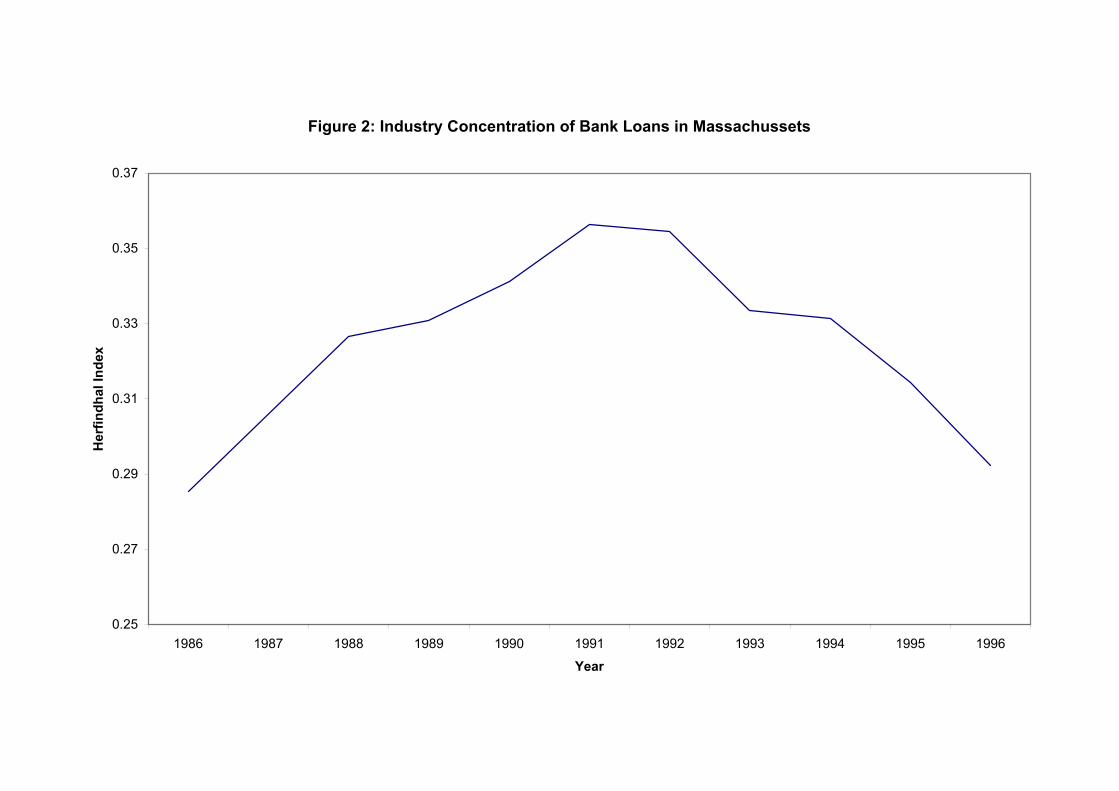
Figure 2: Industry Concentration of Bank Loans in Massachussets

0.25

0.27

0.29

0.31

0.33

0.35

0.37

1986 1987 1988 1989 1990 1991 1992 1993 1994 1995 1996

Year

Her

findh

al In

dex