CE

UeT

DC

olle

ctio

n

A thesis submitted to the Department of Environmental Sciences and Policy of

Central European University in part fulfilment of the

Degree of Master of Science

Investigating potential agricultural-related causes of eutrophication in the Tsimlyansk

Reservoir through GIS and remote sensing

Emily NILSON

May, 2014

Budapest

CE

UeT

DC

olle

ctio

n

ii

Erasmus Mundus Masters Course in

Environmental Sciences, Policy and

Management

MESPOM

This thesis is submitted in fulfillment of the Master of Science degree awarded as a result of successful

completion of the Erasmus Mundus Masters course in Environmental Sciences, Policy and Management

(MESPOM) jointly operated by the University of the Aegean (Greece), Central European University (Hungary),

Lund University (Sweden) and the University of Manchester (United Kingdom).

Supported by the European Commission’s Erasmus Mundus Programme

CE

UeT

DC

olle

ctio

n

iii

Notes on copyright and the ownership of intellectual property rights:

(1) Copyright in text of this thesis rests with the Author. Copies (by any process) either in

full, or of extracts, may be made only in accordance with instructions given by the Author

and lodged in the Central European University Library. Details may be obtained from the

Librarian. This page must form part of any such copies made. Further copies (by any process)

of copies made in accordance with such instructions may not be made without the permission

(in writing) of the Author.

(2) The ownership of any intellectual property rights which may be described in this thesis

is vested in the Central European University, subject to any prior agreement to the contrary,

and may not be made available for use by third parties without the written permission of the

University, which will prescribe the terms and conditions of any such agreement.

(3) For bibliographic and reference purposes this thesis should be referred to as:

Nilson, E. 2014. Investigating potential agricultural-related causes of eutrophication in the

Tsimlyansk Reservoir through GIS and remote sensing. Master of Science thesis, Central

European University, Budapest.

Further information on the conditions under which disclosures and exploitation may take

place is available from the Head of the Department of Environmental Sciences and Policy,

Central European University.

CE

UeT

DC

olle

ctio

n

iv

Author’s declaration

No portion of the work referred to in this thesis has been submitted in support of an

application for another degree or qualification of this or any other university or other institute

of learning.

Emily NILSON

CE

UeT

DC

olle

ctio

n

v

CENTRAL EUROPEAN UNIVERSITY

ABSTRACT OF THESIS submitted by:

Emily NILSON

for the degree of Master of Science and entitled: Investigating potential agricultural-related

causes of eutrophication in the Tsimlyansk Reservoir through GIS and remote sensing.

Month and Year of submission: May, 2014.

Algal blooms can cause disturbances for the many services reliant upon a reliable source of

freshwater, threatening water security. Investigation into the underlying causes of

eutrophication and related algal blooms can be done through the use of ICTs including

remote sensing, GIS, and highly underutilized data portals. Potential agricultural-related

causes of eutrophication in the Tsimlyansk Reservoir in Southern Russia were investigated

with the intention of conducting the preliminary groundwork for future research to be done in

the area. The other primary aims of this research included developing a set of deliverables to

be made available for interested stakeholders and exploring how these ICTs can be used in a

practical application for the region. Eutrophication in the reservoir was investigated through

the development of a detailed land use classification, identification and assessment of algal

blooms through satellite imagery, and exploration into the causal relationship between these

two elements through precipitation. A relationship was found between precipitation and algal

blooms, indicating a potential link between eutrophication and land use in the region around

the reservoir. Further research can build upon this study to conclude on the set of underlying

causes of harmful algal blooms in the reservoir, upon which policies can be based to mitigate

the effects of future occurrences.

Keywords: ICTs, GIS, remote sensing, data portals, land use classification, Tsimlyansk

Reservoir, eutrophication, algal blooms

CE

UeT

DC

olle

ctio

n

vi

Acknowledgements

I would like to express my gratitude to my supervisor Viktor Lagutov for providing

invaluable advice and continued encouragement and support. I give my sincere thanks to

Alexander Prishchepov and to everyone at IAMO for hosting me and providing me with

fundamental knowledge about remote sensing and proper classification techniques. Thank

you to Sergey Stanichny and Ed Bellinger for your valuable help and guidance. And I thank

the MESPOM Consortium for providing me with this opportunity and my fellow batchmates

for making these past two years unforgettable. Thank you, köszönöm, ευχαριστώ, tack.

CE

UeT

DC

olle

ctio

n

vii

Table of Contents

ABSTRACT OF THESIS SUBMITTED BY: .................................................................................... V

ACKNOWLEDGEMENTS ............................................................................................................... VI

TABLE OF CONTENTS ................................................................................................................. VII

LIST OF TABLES .............................................................................................................................. IX

LIST OF FIGURES .............................................................................................................................. X

LIST OF APPENDIX FIGURES....................................................................................................... XI

LIST OF ABBREVIATIONS .......................................................................................................... XII

1. INTRODUCTION ......................................................................................................................... 1

1.1. PROBLEM DEFINITION AND BACKGROUND .............................................................................. 1

1.2. RESEARCH AIM ......................................................................................................................... 3

1.3. RESEARCH QUESTIONS AND OBJECTIVES ................................................................................. 4

1.4. RESEARCH CONSIDERATIONS AND APPROACH ........................................................................ 5

1.4.1. Limitations......................................................................................................................... 5

1.4.2. Methods ............................................................................................................................. 5

1.4.3. Audience ............................................................................................................................ 6

1.4.4. Outline ............................................................................................................................... 6

2. LITERATURE REVIEW ............................................................................................................. 7

2.1. WATER SECURITY: AN INTERNATIONAL CONCERN ................................................................. 7

2.1.1. Freshwater: a Finite Resource .......................................................................................... 7

2.1.2. Water: a Top Policy Agenda Item ..................................................................................... 8

2.1.3. Water Quality: a Prerequisite for Water Security............................................................. 9

2.1.4. Eutrophication ................................................................................................................. 10

2.2. AREA OF STUDY: TSIMLYANSK RESERVOIR ........................................................................... 11

2.2.1. Reservoir Characteristics ................................................................................................ 11

2.2.2. Historical Importance of the Reservoir ........................................................................... 11

2.2.3. The Azov Sea Basin: Economic Importance.................................................................... 13

2.2.4. Importance of Freshwater in the Region ......................................................................... 14

2.2.5. Eutrophication in the Reservoir ...................................................................................... 15

2.2.6. Importance of this Study for the Region .......................................................................... 16

2.3. TECHNOLOGY: REMOTE SENSING .......................................................................................... 16

2.3.1. The Technology ............................................................................................................... 17

2.3.2. Applications for Land Use............................................................................................... 19

2.3.3. Remote Sensing Applications for Water .......................................................................... 20

2.3.4. Applicability of Remote Sensing for the Region .............................................................. 21

2.4. TECHNOLOGY: GEOGRAPHICAL INFORMATION SYSTEMS (GIS) ............................................ 21

2.4.1. GRASS GIS ...................................................................................................................... 21

2.4.2. ArcGIS ............................................................................................................................. 22

2.4.3. Quantum GIS ................................................................................................................... 22

2.5. TECHNOLOGY: DATA PORTALS .............................................................................................. 22

3. METHODOLOGY ...................................................................................................................... 24

3.1. CURRENT LAND USE AND CHANGE (RQ1) ............................................................................. 25

CE

UeT

DC

olle

ctio

n

viii

3.2. EUTROPHICATION IN THE TSIMLYANSK RESERVOIR (RQ2) ................................................... 26

3.3. INVESTIGATING THE RELATIONSHIP (RQ3) ............................................................................ 27

3.4. DELIVERABLES ....................................................................................................................... 28

4. RESULTS AND ANALYSIS ...................................................................................................... 29

4.1. ANALYSIS OF LAND USE AND LAND USE CHANGES (RQ1) ................................................... 29

4.1.1. Land Use Land Cover Classification .............................................................................. 29

4.1.2. Development of a Land Use Thematic Map .................................................................... 45

4.1.3. Determination of Agricultural Land Use Change ........................................................... 46

4.1.4. Summarizing Work Conducted for RQ1 .......................................................................... 49

4.2. ANALYSIS OF EUTROPHIC ALGAL BLOOMS (RQ2) ................................................................. 50

4.2.1. Identification of Eutrophication Events .......................................................................... 50

4.2.2. Determination of the Extent of Identified Algal Blooms ................................................. 52

4.2.3. Summarizing Work Conducted for RQ2 .......................................................................... 56

4.3. FINDING RELATIONSHIPS (RQ3) ............................................................................................. 57

4.3.1. Investigation into Precipitation-Induced Algal Blooms .................................................. 57

4.3.2. Summarizing Work Conducted for RQ3 .......................................................................... 61

5. DISCUSSION ............................................................................................................................... 62

5.1. RESEARCH RESULTS AND LIMITATIONS ................................................................................. 62

5.1.1. Land Use Classification .................................................................................................. 62

5.1.2. Land Use Change ............................................................................................................ 63

5.1.3. Land Use Map ................................................................................................................. 63

5.1.4. Identification of Algal Blooms......................................................................................... 64

5.1.5. Comparing Land Use and Algal Blooms Through Precipitation .................................... 64

5.2. PATHWAYS FOR FURTHER RESEARCH .................................................................................... 65

6. CONCLUSION ............................................................................................................................ 66

REFERENCES .................................................................................................................................... 68

PERSONAL COMMUNICATIONS ................................................................................................. 72

GIS DATA SOURCES ....................................................................................................................... 72

APPENDICES ..................................................................................................................................... 73

CE

UeT

DC

olle

ctio

n

ix

List of Tables Table 1. Research objectives and corresponding tasks and methods. .................................................................. 25

Table 2. Eight Landsat tiles selected for land use cover classification. Data source: (USGS 2014) .................... 31

Table 3. Landsat 5 Thematic Mapper band characteristics. Data source: (USGS 2013). .................................... 32

Table 4. Land use land cover classes for classification. ....................................................................................... 34

Table 5. Number of polygon trainings and pixels developed for the second classification. ................................ 39

Table 6. Points per class sampled in the classification process. ........................................................................... 43

Table 7. Algal bloom extent criteria. ................................................................................................................... 52

Table 8.Satellite-identified algal blooms with a "High" bloom extent. ................................................................ 54

Table 9. Temporal distribution (by month) of identified algal blooms. ............................................................... 55

CE

UeT

DC

olle

ctio

n

x

List of Figures Figure 1. Map of the Tsimlyansk Reservoir in Southern Russia. (Map created by author). ................................ 12

Figure 2. Electromagnetic spectrum. (Created by author based on Chuvieco and Huete 2010). ......................... 17

Figure 3. Flow chart illustrating overall research plan. ....................................................................................... 24

Figure 4. Example of algal bloom in satellite imagery (USGS 2014). ................................................................ 27

Figure 5. Four Landsat tiles selected for land use classification. (USGS 2014). ................................................. 31

Figure 6. Clipping the 80 km buffer zone, developed in ArcMap, from the Landsat tile mosaics. ..................... 33

Figure 7. Buffer zone around the reservoir encompassing parts of Rostov and Volgograd oblasts. (Map created

by author). ................................................................................................................................................... 34

Figure 8. Screenshot taken while developing training polygons using high-resolution images on Google Earth

and ArcMap. ............................................................................................................................................... 35

Figure 9. Comparison of spectral signatures of agricultural land in June versus August(USGS 2014). .............. 36

Figure 10. First (and unsuccessful) MLC output viewed in ArcMap. (Map created by author). ......................... 38

Figure 11. Second (and final) MLC output viewed in ArcMap. (Map created by author). .................................. 39

Figure 12. 600 random points used for classification validation. (Map created by author). ................................ 41

Figure 13. Screenshot taken while conducting random point validation using Google Earth and ArcMap. ....... 42

Figure 14. Screenshot taken of a zoomed in representation of random point validation using Google Earth and

ArcMap. ...................................................................................................................................................... 42

Figure 15. Kappa analysis output: error matrix. .................................................................................................. 44

Figure 16. Cropland as a percentage of total land area, 1995 to 2009. Data source: (ROSSTAT 2010) ............. 46

Figure 17. Grain and forage crops as the predominant crops in the region. Data source: (ROSSTAT 2010) ..... 47

Figure 18. Volgograd grain and forage crop yields (excluding sugar beets) from 1995 to 2009. Data source:

(ROSSTAT 2010) ....................................................................................................................................... 48

Figure 19. Rostov grain and forage crop yields (excluding sugar beets) from 1995 to 2009. Data source:

(ROSSTAT 2010) ....................................................................................................................................... 48

Figure 20. Sugar beet yields for both oblasts from 1995 to 2009. Data Source: (ROSSTAT 2010) ................... 49

Figure 21. Final land use map. (Map created by author). .................................................................................... 50

Figure 22. Screenshot from the NASA Ocean Color Level 3 Browser. Image from: (NASA 2014) .................. 56

Figure 23. Screenshot showing the geographical extent of Giovanni precipitation data. Image from: (NASA

2013a) ......................................................................................................................................................... 58

Figure 24. Precipitation vs. algal blooms for 2003. Data source: (NASA 2013a; USGS 2014) .......................... 59

Figure 25. Precipitation vs. algal blooms for 2000. Data source: (NASA 2013a; USGS 2014) .......................... 59

Figure 26. Precipitation vs. algal blooms for 2001. Data source: (NASA 2013a; USGS 2014) .......................... 60

Figure 27. Precipitation vs. algal blooms for 2012. Data source: (NASA 2013a; USGS 2014) .......................... 60

CE

UeT

DC

olle

ctio

n

xi

List of Appendix Figures Appendix Figure 1. Landsat image catalogue: May to October 2008-2010. Data Source: (USGS 2014) .......... 73

Appendix Figure 2. Screenshots of www.azovcenter.ru showing published Landsat imagery list ..................... 80

Appendix Figure 3. Total cropland (in thousands of hectares) in Rostov and Volgograd oblasts. Data Source:

(ROSSTAT 2010) ....................................................................................................................................... 81

Appendix Figure 4.Algal bloom events seen in Landsat images. Data Source: (USGS 2014) ........................... 82

Appendix Figure 5. Screenshots of www.azovcenter.ru showing published algal bloom images identified

through satellite imagery. ............................................................................................................................ 89

Appendix Figure 6. Determination of algal bloom extent. ................................................................................. 90

Appendix Figure 7. Precipitation vs. algal bloom graphs, 1998-2013. Data Source: (USGS 2014; NASA 2013a)

.................................................................................................................................................................... 92

CE

UeT

DC

olle

ctio

n

xii

List of Abbreviations

ETM+ Landsat 7 Enhanced Thematic Mapper Plus

GIS Geographic Information Systems

IAMO Leibniz Institute of Agricultural Transition Economies

ICT Information and Communication Technologies

MLC Maximum likelihood classification

MODIS Moderate Resolution Imaging Spectroradiometer (satellite sensor)

NASA National Aeronautics and Space Administration

NIR Near infrared (electromagnetic spectrum)

SPOT Satellite Pour l‘Observation de la Terre (satellite)

SWIR Short wave infrared (electromagnetic spectrum)

TM Landsat 5 Thematic Mapper

UN United Nations

UNEP United Nations Environment Programme

USGS United States Geological Survey

CE

UeT

DC

olle

ctio

n

1

1. Introduction

1.1. Problem Definition and Background

Issues regarding water security and water quality have garnered attention on an

international level for many years. The threatened status of freshwater in many areas of the

world is of great concern and has been a key focal point of international, national, and local

policies around the world. Eutrophication remains one of the most pressing issues in the

protection of freshwater ecosystems (Schindler 2006). Extensive episodes of eutrophication,

e.g. in the form of algal blooms, is one of the many parameters that affects water quality.

Algal blooms can produce toxins harmful to human health and can disrupt the ecosystem

services that are dependent on a reliable source of freshwater.

The Tsimlyansk Reservoir in Southern Russia is of great environmental and economic

importance to the region in which it is located. It is relied upon as a source of freshwater in an

area that is densely populated, is used extensively for irrigation of the region‘s agricultural

lands, and is a source of cooling water for a nuclear power plant in the area, among a variety

of other uses (Lagutov and Lagutov 2012). But in recent years, harmful algal blooms have

been reported and associated with a number of environmental and economic concerns. Major

fish kills have occurred in the past few years, including one in 2010 in which approximately

900,000 fish were found dead in the reservoir. Similar instances of fish kills occurred in May

2007 and June and August 2009 (Vesti 2011). In October 2009, a particularly bad algal bloom

occurred, clogging filters at a water treatment plant and leaving about 170 thousand people

without water for 3 days (Nikanorov et al. 2010). These major events were caused by algal

blooms occurring as a result of increased eutrophication in the reservoir. In order to address

this issue to be able to develop policies and practices to mitigate future occurrences of this

CE

UeT

DC

olle

ctio

n

2

kind, research must be conducted to determine the underlying causes of these harmful algal

blooms in the reservoir.

Agricultural runoff containing nitrogen and phosphorus is a well-recognized source of

eutrophication in freshwater systems (Serediak et al. 2014; Ferreira et al. 2011). The

Tsimlyansk Reservoir is in a region of high agricultural importance, deemed the nation‘s

―breadbasket‖ (Lagutov and Lagutov 2012). Because of the developed agriculture in the area,

it is reasonable to assume there is a connection between the agricultural lands and the

eutrophication events in the reservoir, but preliminary research must be conducted to

determine if the agricultural lands in the region are indeed related to these events, which will

set the foundation for how to address the problem on a higher level.

Remote sensing and geographic information systems (GIS) are two types of technologies

among the ever-increasing pool of information and communication technologies (ICTs) that

have proven to be useful to study environmental problems such as this, for both land

(Kuemmerle et al. 2013) and water applications, including investigation into eutrophication of

freshwater ecosystems (Ritchie et al. 2003; Kitsiou and Karydis 2011; Barnes et al. 2014;

Brivio et al. 2001; Farag and El-Gamal 2011). Furthermore, there are numerous large

repositories devoted to data derived from remote sensing technologies (e.g. data portals) that

are available online and that provide free access to tremendous amounts of data. These

resources, the number of which is constantly increasing, are highly underutilized, despite the

wealth of information they contain. This research is using the opportunity to combine remote

sensing and GIS technologies and the vast amount of available data and explore how they be

used to investigate the problem of eutrophication in the area around the Tsimlyansk

Reservoir.

In order to investigate this issue using the aforementioned methods, an important step is

to accurately determine the state of land cover (used interchangeably with ―land use‖ in this

CE

UeT

DC

olle

ctio

n

3

study) in the region at the time these large-scale algal bloom events were taking place (around

2010). Detailed land cover data is a critical part of investigating environmental phenomena

(Heinl et al. 2009). As such, a large portion of this research is aimed at developing detailed

and accurate land cover data for this region, which will serve as a foundation for future

research and analysis. Next, eutrophication in the reservoir is investigated to identify when

and to what extent algal blooms have occurred in recent years. Lastly, the relationship

between land use and eutrophication is investigated through precipitation data, providing an

example of how to use the data that has been gathered to attempt to determine a causal link

between the two elements.

To date, very little work has been done to research this issue and determine the

underlying causes of it, especially with the use of ICTs and data portals. Furthermore, the

deliverables that will be created as a result of this research, which do not yet freely exist, will

be made publicly available to provide useful data to interested stakeholders in the region. Not

only will this research contribute to the limited literature on the topic, especially literature in

the English language in which there is little written currently, but it will set the foundation for

future research to be conducted, which will be able to be used as a scientific basis for

policymaking and decision-making in the future. It will also provide an example of how the

vast amount of data available can be utilized using available technologies in a practical and

useful manner.

1.2. Research Aim

Since there has been little to no work done in this field so far for the region, one of the

main goals of this study is to conduct the preliminary groundwork for future research and to

generate a set of deliverables that can be used and expanded upon for environmental

assessments, environmental monitoring, and policymaking regarding land use around and

water quality of the Tsimlyansk Reservoir in the future. In addition to developing the

CE

UeT

DC

olle

ctio

n

4

foundation for future research and making some data publicly available, another primary goal

of this research is to make use of remote sensing and GIS technologies as well as to utilize

and explore the tremendous amount of data freely available through data portals.

1.3. Research Questions and Objectives

The aforementioned research aims will be pursued through the lens of the following

research questions (RQ) and corresponding objectives (OB):

RQ1: What was the state of land use around the Tsimlyansk Reservoir around the time of

reported harmful algal blooms? Has it changed much over the past 15 years?

OB1: Obtain data indicating land use in the area around the reservoir in 2010.

OB2: Develop a land use thematic map of land use in 2010 that can be used as a basis

for future research in the region.

OB3: Determine how land use in the area around the reservoir has changed in the past

15 years.

RQ2: When and to what extent have algal blooms occurred in the Tsimlyansk Reservoir in the

past 15 years?

OB1: Identify instances of algal blooms in the reservoir.

OB2: Determine the extent of identified blooms and develop a catalogue of available

data that can be used for future research.

RQ3: How can this data be used to investigate the relationship between land use and

eutrophication in the Tsimlyansk Reservoir?

OB1: Investigate the link between land use and eutrophication through precipitation

data and determine if algal blooms occur after large episodes of precipitation.

CE

UeT

DC

olle

ctio

n

5

1.4. Research Considerations and Approach

1.4.1. Limitations

A limitation for this study was that the researcher does not speak Russian and was thus

not able to access a wide variety of information that could have been useful and interesting to

the research. But as this limitation was identified at the beginning of the research period,

efforts were taken to focus on study methods that would not require Russian language skills,

namely remote sensing and GIS. Furthermore, as mentioned above, this limitation provided

the opportunity to utilize some of the ever-increasing amount of data and ICTs to address a

real environmental problem in the region.

Another limitation was the availability of region-specific data (data that cannot be

derived from remote sensing) for the topic and for the study area. As will be discussed in

Section 2 of this study, there is a very limited amount of information regarding water quality

in the reservoir. Furthermore, government statistics on land use and agricultural productivity

are not readily accessible for certain regions within the study area. This limitation was

addressed by focusing on the use of readily available data (e.g. satellite imagery of the region)

and data from trusted sources (e.g. statistics that were able to be obtained from government

databases and GIS datasets from researchers in the region), all of which can be used and

analysed with remote sensing and GIS technologies.

1.4.2. Methods

This study will address the aforementioned research questions through a combination of a

brief literature review, a study visit to learn remote sensing techniques and how to perform

land use classification, the gathering of data from data portals, and the use of remote sensing

and GIS technologies and analysis of statistics.

CE

UeT

DC

olle

ctio

n

6

1.4.3. Audience

As mentioned in Section 1.2, one of the primary aims of this research is to conduct the

preliminary data preparation and analysis on the issue of agricultural-related eutrophication in

the Tsimlyansk Reservoir using remote sensing and GIS. This research is intended for use by

stakeholders in the Azov Sea basin, particularly environmental and water practitioners and

policymakers. Those individuals and organizations could use this research as a basis for

further research and analysis on the causes of eutrophication in the reservoir, which would

serve as a basis for mitigation efforts to combat harmful algal blooms in the future and

preserve the reservoir. Some of the deliverables produced as a result of this research will be

made publicly available on the Azov Basin Center website (http://azovcenter.ru/), a website

devoted to promoting the sustainable development of the region, so they can be of immediate

use to interested stakeholders.

1.4.4. Outline

Section 2 (Literature Review) of this study includes a literature review covering 5 topics:

the importance and relevance of water security in current policy discussion and the role

eutrophication plays; an overview of the study area and the importance of the Tsimlyansk

Reservoir to the region and economy; the suitability of remote sensing for both land and water

applications; and an overview of the GIS software packages and data portals used for

research. Section 3 (Methodology) provides the research design and describes the basic

methodological steps that will be taken to conduct the research, broken down into each

research question. Section 4 (Results and Analysis) discusses the specific steps taken to

conduct the research, what exactly was done, and what results were obtained. Section 5

(Discussion) provides a discussion of the results, limitations, and highlights a number of

pathways for further research. Section 6 (Conclusion) concludes the research by providing an

overview of what work was performed and what was achieved.

CE

UeT

DC

olle

ctio

n

7

2. Literature Review

2.1. Water Security: an International Concern

Water security is an important issue on the international policy agenda and is a focal

point across all levels of government and interests, from global environmental publications to

national and local agreements and legislation. Freshwater is an increasingly finite resource

and there are a number of parameters that threaten the quality of freshwater ecosystems

including eutrophication, which can lead to harmful algal blooms and pose threats to human

health and damage to infrastructure. This section will introduce the concept of water security,

highlight its importance in the current political arena, and discuss how it relates to water

quality.

2.1.1. Freshwater: a Finite Resource

Freshwater ecosystems provide a myriad of services that help sustain human existence.

They include both provisioning services and supporting services, as defined by the

Millennium Ecosystem Assessment (Reid et al. 2005). Freshwater ecosystems provide people

with water for a variety of uses, including drinking, sanitation, industry, and agriculture,

among others. But the existence and availability of freshwater also supports other ecosystem

processes, making life on Earth possible (Reid et al. 2005).

Of all the water available on Earth, freshwater makes up only 2.5%, the majority of

which is inaccessible because it is perennially frozen. Most of the world‘s liquid freshwater is

groundwater. A mere 0.26% makes up the rivers, lakes, and reservoirs around the globe.

Approximately 75% of human water withdrawals (e.g. for drinking, agriculture, industry, and

other uses) come from surface freshwaters in this 0.26% (Carpenter et al. 2011). Human

activities and human-induced climate change are changing freshwater ecosystems and

CE

UeT

DC

olle

ctio

n

8

threatening to cause problems for the world‘s population in the future. Freshwater is an

increasingly finite resource and its importance for sustaining human life and its uneven

distribution in both space and time has made water scarcity a permanent issue on the political

agenda.

2.1.2. Water: a Top Policy Agenda Item

Issues regarding water availability and quality have consistently been a focal point of

both international and national policy in recent years. Having access to water of an acceptable

quality for drinking and sanitation was declared a human right by the United Nations (UN)

General Assembly in 2010 (UN General Assembly 2010).

Water is a recurring theme in a number of global policy documents and reports. The

UN‘s Millennium Development Goals incorporate water access into Target 7.C, part of Goal

7, which aims to ―Ensure Environmental Sustainability‖. The target, aiming to halve the

"proportion of the population without sustainable access to safe drinking water and basic

sanitation‖ by 2015 was met in 2010 (UN 2013). But despite this progress, millions will still

be without safe drinking water by the end of the target‘s time period (UNEP 2012).

In addition, water is a main theme in the United Nations Environment Programme‘s

(UNEP) Global Environmental Outlook 5 report, which was released in 2012. This report

notes the need for improved governance of water resources to combat competing water uses

and overexploitation from various actors (UNEP 2012).

Many international agreements and policy documents have been developed over the past

few decades (e.g. Johannesburg Plan of Implementation, the Dublin Principles, the UN

Millennium Declaration) that deal with water issues from various angles: the importance of

water ecosystems, water‘s impact on human well-being, how to use water the most efficiently,

how to improve and sustain water quality, and how to adequately manage water resources

(UNEP 2012). But there have also been many declarations and pieces of legislation on the

CE

UeT

DC

olle

ctio

n

9

regional and national level, like the European Union‘s (EU) Water Framework Directive (EU

Directive 2000) that have similar goals.

Because of water‘s transboundary nature, the only way to effectively manage the

resource is through cross-border, cross-sectoral and multi-actor coordination. The concept of

Integrated Water Resource Management, based on the Dublin Principles, began to garner

attention after the Earth Summit in 1992. The concept stresses the importance of coordination

and cooperation across all levels (Agarwal et al. 2000).

To conclude, water is a top priority item in the international policy arena. It is reflected

in legislation on all levels of government and is a well-recognized issue of importance.

2.1.3. Water Quality: a Prerequisite for Water Security

―Water quality‖ can be hard to define because it depends on the ultimate use of the

water: water intended for human consumption would inevitably have a different definition

than water intended for agricultural or industrial purposes (Ritchie et al. 2003). An attempt to

define water quality (referred to as ―ecological status‖) is made in Annex V of the EU Water

Framework Directive, which takes into consideration a number of factors in its definition:

biological (e.g. flora and fauna) hydromorphological (e.g. dynamics associated with water

flow), chemical (e.g. presence of pollutants), and other characteristics like thermal conditions,

oxygenation, salinity, acidification, and nutrient conditions (EU Directive 2000).

Water quality is a necessary prerequisite to attaining water security, but similar to ―water

quality‖, developing an accepted definition for ―water security‖ has been difficult (UNEP

2012). For the purposes of this study, the definition of water security will come from the

Ministerial Declaration of The Hague, agreed to in 2000, which was relied upon by the UNEP

Global Environmental Outlook 5 report. The Declaration defines water security as:

―ensuring that freshwater, coastal and related ecosystems are protected and

improved; that sustainable development and political stability are promoted, that

every person has access to enough safe water at an affordable cost to lead a healthy

CE

UeT

DC

olle

ctio

n

10

and productive life and that the vulnerable are protected from the risks of water

related hazards‖ (World Water Council 2000).

Water security is inherently associated with water quality in the aforementioned

definition, as ecosystems need to be protected and improved, which denotes a certain level of

quality, and people need to have access to safe water, indicating an even higher level of

quality necessary.

2.1.4. Eutrophication

While there are many indicators of water quality as discussed earlier in this section (e.g.

hydromorphology, salinity, thermal conditions), eutrophication remains one of the most

pressing issues in the protection of freshwater and marine ecosystems (Schindler 2006).

Eutrophication is a predominantly anthropogenic-caused phenomenon that occurs when

surface waters are enriched with nutrients, mainly nitrogen and phosphorus (Serediak et al.

2014; Ferreira et al. 2011). It is widely accepted that agriculture and urban activity are the two

major causes of eutrophication from non-point sources in aquatic ecosystems. Agricultural

runoff is rich in both nitrogen (N) and phosphorus (P) from fertilizers and pesticides applied

to crops. Runoff from these lands is known to cause problems associated with eutrophic water

conditions, like harmful algal blooms, oxygen depletion, and fish kills, among others

(Carpenter et al. 2011; Carpenter et al. 1998). But the factors involved in the development of

eutrophic algal blooms are inherently complex. Regarding agricultural runoff, there are

numerous factors involved in if, how, and when an algal bloom occurs including, for example,

the presence of limiting nutrients; episodes of precipitation; thermal stratification in the body

of water; the particular species of algae; when, how much, and what type of fertilizer was

applied; among many other components (Bellinger 2014).

The nutrient enrichment of freshwater ecosystems caused by eutrophication diminishes

water quality and threatens its ability to be used for human consumption, agriculture, and

CE

UeT

DC

olle

ctio

n

11

industry. In freshwater ecosystems, eutrophication is often exhibited through blooms of

cyanobacteria (blue-green algae), which can pose a health risk to humans (Carpenter et al.

1998). This research will focus on problems associated with eutrophication in a freshwater

reservoir. While eutrophication is just one aspect of water quality, and quality only part of

water security, it is still important to address because of the economic and environmental

consequences that can, and have been, arising from it in the area of study.

2.2. Area of Study: Tsimlyansk Reservoir

As major eutrophication events have been occurring in recent years and causing

disturbances in the region, this research is focused on eutrophication in the Tsimlyansk

Reservoir. The following section will describe the region in which the reservoir is located and

highlight important economic and environmental characteristics.

2.2.1. Reservoir Characteristics

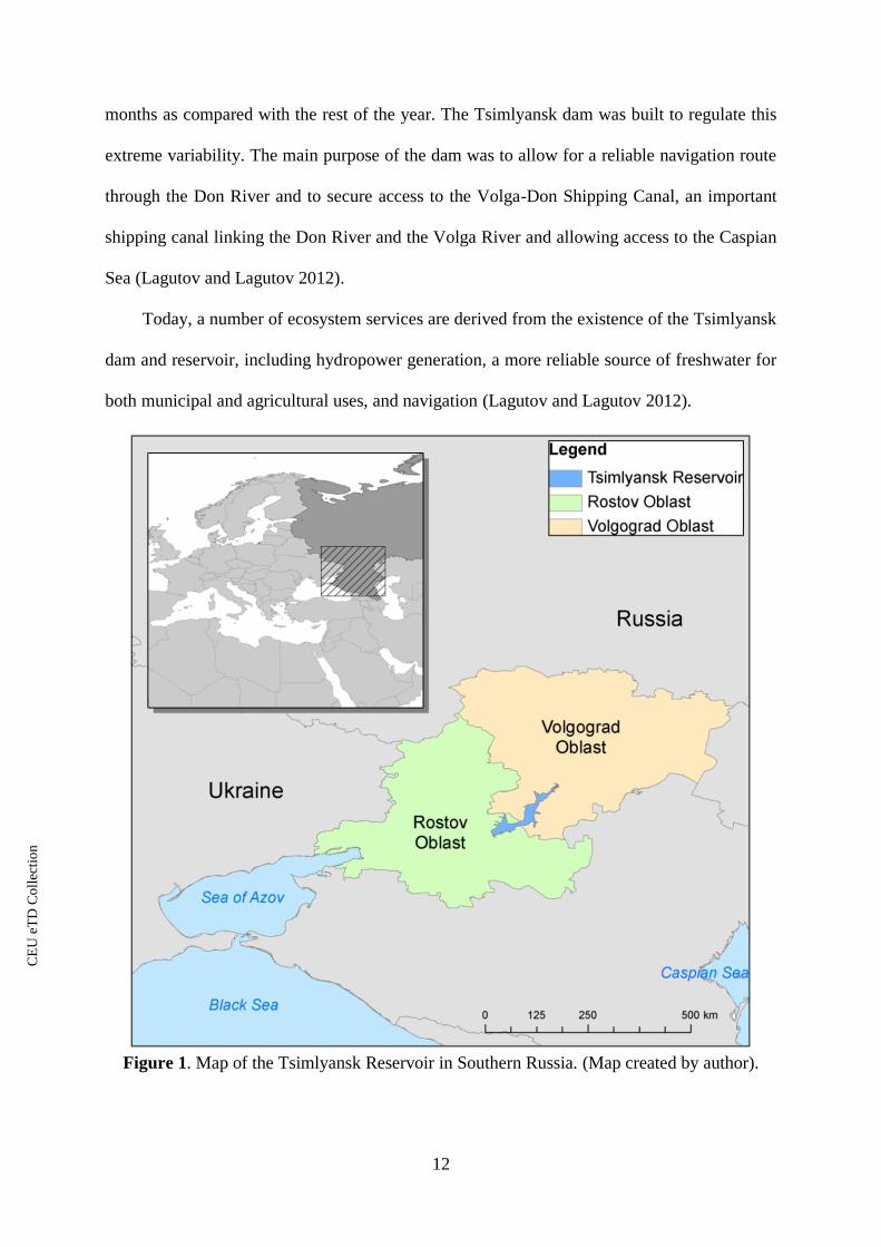
The Tsimlyansk Reservoir is located in Southern Russia, northeast of the Black Sea and

the Azov Sea, as seen in Figure 1. It falls between two regions, called ―oblasts‖, Rostov to

the west and Volgograd to the east. It is the largest freshwater body in the basin of the Azov

Sea (Gilfanova 2012), measuring 260 kilometres in length and having a surface area of 2,702

square kilometres (Novikova et al. 2012). At full capacity, the volume of the reservoir is 23.9

cubic kilometres and it has a maximum depth of 36 meters (Lagutov and Lagutov 2012).

2.2.2. Historical Importance of the Reservoir

The reservoir was formed as a result of the Tsimlyansk dam, which was built as a part of

the ‗Great Construction Projects of Communism‘ and began operation in 1953. The dam was

built to regulate the Don River, the largest river in the Azov Sea basin. The Don River is

characterized by extreme variability in its annual water distribution. About 70% of the total

river flow in the Don is comprised of snowmelt, causing tremendous discharge in the spring

CE

UeT

DC

olle

ctio

n

12

months as compared with the rest of the year. The Tsimlyansk dam was built to regulate this

extreme variability. The main purpose of the dam was to allow for a reliable navigation route

through the Don River and to secure access to the Volga-Don Shipping Canal, an important

shipping canal linking the Don River and the Volga River and allowing access to the Caspian

Sea (Lagutov and Lagutov 2012).

Today, a number of ecosystem services are derived from the existence of the Tsimlyansk

dam and reservoir, including hydropower generation, a more reliable source of freshwater for

both municipal and agricultural uses, and navigation (Lagutov and Lagutov 2012).

Figure 1. Map of the Tsimlyansk Reservoir in Southern Russia. (Map created by author).

CE

UeT

DC

olle

ctio

n

13

2.2.3. The Azov Sea Basin: Economic Importance

The region in which the reservoir is located, the Azov Sea basin, is a notably important

economic region in both Russia and Ukraine. The basin encompasses a high level of

agricultural development, including both cropland and livestock farming. The majority of the

watershed is covered in cultivated lands. The region is known for its fertile soils (called

chernozem) and favourable climate, making it the ―breadbasket‖ of Russia. But the region is

semi-arid and there is low precipitation in the entire basin and even less in the eastern areas,

necessitating high amounts of freshwater abstraction for irrigation (Lagutov and Lagutov

2012). In the lower Don River are, there are approximately 323,000 hectares of irrigated

lands, requiring a volume of about 2 cubic kilometres of water each year (Shavrak et al.

2012), or approximately 8% of the total capacity of the reservoir itself (calculated by author).

As mentioned above, transportation is another important economic factor in the region.

The basin is located in the middle of many important shipping and transportation routes in the

region (Lagutov and Lagutov 2012). The use of the reservoir for shipping and transportation

is increasing: a total of 5,022 ships passed through the reservoir in 2000, which increased to

6,799 ships in 2007 (Shavrak et al. 2012). The increasing traffic cannot be supported by the

existing Volga-Don Shipping Canal and there are two canal construction proposals currently

under discussion (Lagutov and Lagutov 2012).

Additionally, power generation is important in the region. The Tsimlyanskaya

hydropower station generates energy, albeit a relatively small amount compared to other

stations in Southern Russia. The reservoir is also used to provide cooling water to the

Volgodonsk Nuclear Power Plant located there. The basin is densely populated, particularly

along the rivers, and is one of the most densely populated regions in both countries. The Azov

Sea used to be an important fishery, but overexploitation and unsustainable fisheries

management caused the regional fishing industry to collapse, turning what was once touted as

CE

UeT

DC

olle

ctio

n

14

one of the most productive seas in the world to one in which fish stocks are at critical levels

(Lagutov and Lagutov 2012).

The freshwater in this region, particularly that of the Don River and Tsimlyansk

Reservoir, allows all of these things to happen – the agricultural productivity, shipping

transportation, power generation, and supporting a large population with drinking water and

other important services. The region is dependent on the availability of this freshwater.

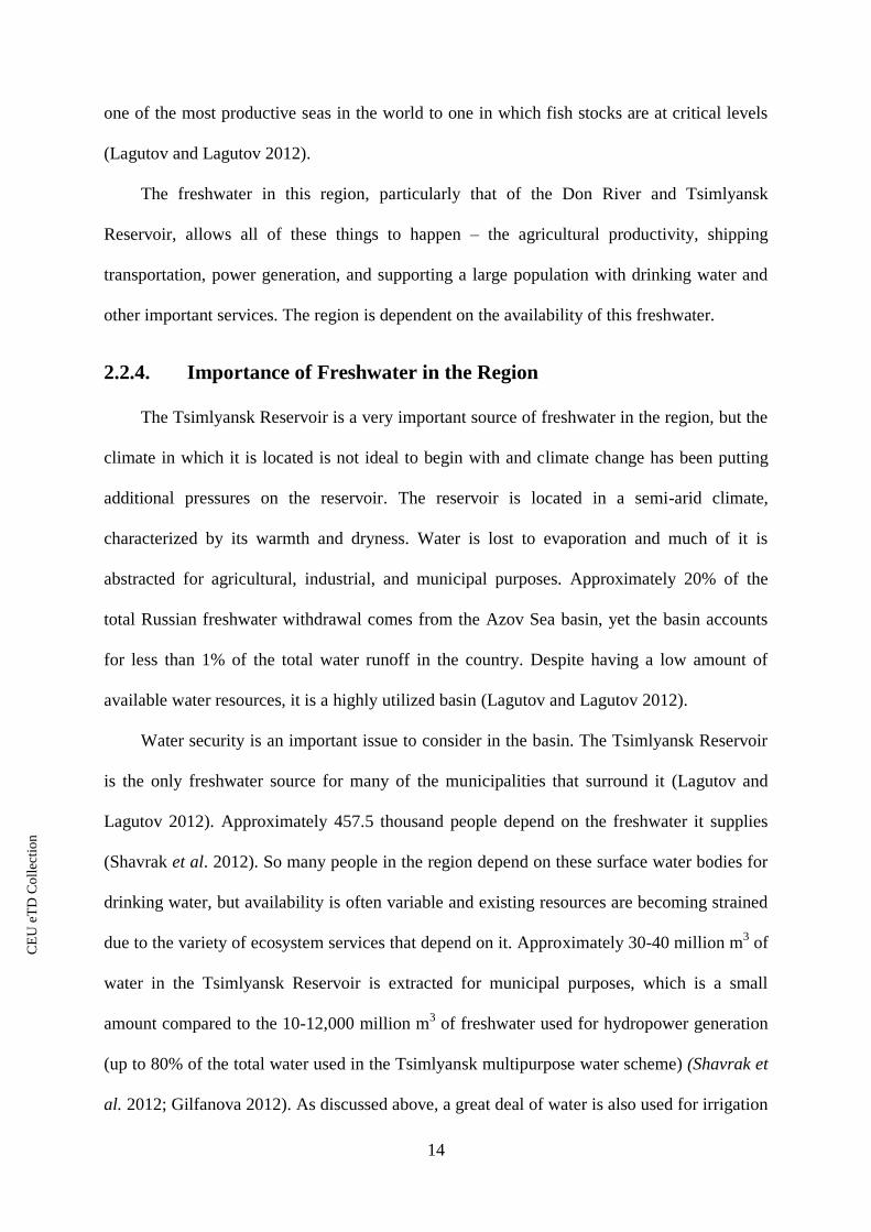
2.2.4. Importance of Freshwater in the Region

The Tsimlyansk Reservoir is a very important source of freshwater in the region, but the

climate in which it is located is not ideal to begin with and climate change has been putting

additional pressures on the reservoir. The reservoir is located in a semi-arid climate,

characterized by its warmth and dryness. Water is lost to evaporation and much of it is

abstracted for agricultural, industrial, and municipal purposes. Approximately 20% of the

total Russian freshwater withdrawal comes from the Azov Sea basin, yet the basin accounts

for less than 1% of the total water runoff in the country. Despite having a low amount of

available water resources, it is a highly utilized basin (Lagutov and Lagutov 2012).

Water security is an important issue to consider in the basin. The Tsimlyansk Reservoir

is the only freshwater source for many of the municipalities that surround it (Lagutov and

Lagutov 2012). Approximately 457.5 thousand people depend on the freshwater it supplies

(Shavrak et al. 2012). So many people in the region depend on these surface water bodies for

drinking water, but availability is often variable and existing resources are becoming strained

due to the variety of ecosystem services that depend on it. Approximately 30-40 million m3 of

water in the Tsimlyansk Reservoir is extracted for municipal purposes, which is a small

amount compared to the 10-12,000 million m3 of freshwater used for hydropower generation

(up to 80% of the total water used in the Tsimlyansk multipurpose water scheme) (Shavrak et

al. 2012; Gilfanova 2012). As discussed above, a great deal of water is also used for irrigation

CE

UeT

DC

olle

ctio

n

15

purposes. Additionally, much water is lost through evaporation due to the semi-arid climate

and the reservoir‘s large surface area (Lagutov and Lagutov 2012). The amount of water

being lost through evaporation is increasing as well. Between 1953-1987, evaporated water

amounted approximately 11% of the water input. From 2000-2009, that amount had increased

to 14%, signifying an increasing trend. This is consistent with increasing air temperatures in

the region, which have increased by 1.7ºC in the last 25 years (Shavrak et al. 2012).

Furthermore, freshwater in the region has been found to contain high levels of pollution.

About 7.6% of samples in the region contained biological contaminants. Approximately

10,000 people in the area drink untreated water from the surface water bodies, often exposing

themselves to these contaminants. There are already public health threats arising in the area

(Lagutov and Lagutov 2012).

In summary, the reservoir is depended upon for many purposes. Recent algal blooms and

associated problems have threatened the services it provides, threatening water security in the

region overall.

2.2.5. Eutrophication in the Reservoir

Eutrophication is an important issue for the Tsimlyansk Reservoir. As defined earlier in

the chapter, when a water body becomes eutrophic, which occurs when it receives excess

nutrients, it often results in the development of blue-green algae, sometimes creating algal

blooms. This can often occur because of agricultural runoff that contains phosphorus- and

nitrogen-based fertilizers and organic matter (Novikova et al. 2012).

The nutrient content, predominantly nitrogen and phosphorus, in the Tsimlyansk

Reservoir is high enough that the water body can be considered ‗hypertrophic‘. But there is

not reliable or consistent water quality or nutrient concentration data for the reservoir. There

was some testing done in the 1980s, some in 1990, and some between 2006-7, but the data is

inconsistent. From the testing that has been done, it was found that nutrient concentrations

CE

UeT

DC

olle

ctio

n

16

exceeded the maximum permissible concentration every year in 38-100% of the samples

(Nikanorov et al. 2012).

There are typically two peaks during the year of blue-green algae in the reservoir as a

result of eutrophication, the first in the spring (Bacillariophyta) and the second in the late

summer (Cyanophyta). The algae are highly productive and a bloom can reach up to 80% of

the reservoir‘s surface area (Nikanorov et al. 2012). As mentioned in Section 1 of this study, a

number of problems resulting from algal blooms have occurred in recent years, including fish

kills (Vesti 2011) and damage to water treatment infrastructure, the latter of which left about

170 thousand of people without water to drink for 3 days during a particularly large algal

bloom in October 2009 (Nikanorov et al. 2010).

Eutrophication is a major problem in the reservoir and there has not been adequate work

done to address the issue in order to mitigate problems from future occurrences.

2.2.6. Importance of this Study for the Region

The Tsimlyansk Reservoir is located in a region characterized for its semi-arid climate

and low precipitation. The reservoir is heavily utilized and is relied upon for a multitude of

services, from providing drinking water to area inhabitants to irrigating the highly developed

agricultural areas in the region. Eutrophication and resulting algal blooms are causing

problems in the region, necessitating the need for research into the underlying causes of the

blooms so mitigation options can be pursued. Remote sensing and GIS are two ICTs that can

be used to learn more about the problem and get closer to finding solutions to address it.

2.3. Technology: Remote Sensing

Remote sensing and subsequent processing and analysis made up a large portion of this

research. This section will describe the technology and how it can be used in land and water

applications.

CE

UeT

DC

olle

ctio

n

17

2.3.1. The Technology

Remote sensing can be defined as the acquisition of information about an object without

being in direct contact with that object (Chuvieco and Huete 2010; Gibson and Power 2000;

Weng 2013). In essence, it is the act of ―sensing‖ and recording information about an object

while being at a distance (e.g. a place that is ―remote‖) from it (Weng 2013).

The human eye can only perceive a small part of the electromagnetic spectrum, which

can be defined as the range of all of the various types of electromagnetic radiation that exist.

The small portion we can perceive is called the visible spectrum and ranges from 0.4 to 0.7

micrometers (μm), as seen in Figure 2, based on Chuvieco and Huete (2010). Through remote

sensing technology, we can expand the portion of the electromagnetic spectrum that we can

perceive beyond this visible region. Different portions of the electromagnetic spectrum have

different uses in remote sensing. For example, the near-infrared (NIR) portion is often used to

study green vegetation, while the short wave infrared (SWIR) portion of the middle infrared

range is often used in soil vegetation studies (Chuvieco and Huete 2010).

Figure 2. Electromagnetic spectrum. (Created by author based on Chuvieco and Huete 2010).

Objects on the Earth‘s surface (as well as different types of land cover) act differently in

the various parts of the electromagnetic spectrum. They have unique ―spectral signatures‖,

which is a term that means the amount of reflectance an object gives off at different parts of

CE

UeT

DC

olle

ctio

n

18

the spectrum. Water, for example, has a completely different spectral signature than green

vegetation because it has different levels of reflectance at various wavelengths in the spectrum

(Chuvieco and Huete 2010). Because of these spectral differences, it is possible to use remote

sensing to detect the type of land cover on the Earth‘s surface based on the land cover‘s

specific spectral signature.

Remote sensing is not a new concept: it has been used since the early 1960s to acquire

information about the Earth from aerial photography (Chuvieco and Huete 2010). But the

term has evolved to cover many more technologies and platforms since then. Images can be

obtained through instruments aboard aircraft or balloons or instruments mounted on space-

borne platforms, like satellites (Weng 2013). And the data these instruments acquire have

become much more sophisticated, spanning a wider range of the electromagnetic spectrum

well beyond the visible part of it.

This study will focus on satellite remote sensing because of the advantages space-based

observations have over other platforms. According to Chuvieco and Huete (2010), some of

these advantages include:

A comprehensive and consistent view of the entire Earth

A variety of space-based instruments that have a wide range of technological

capabilities (e.g. spatial resolution)

The ability to obtain information from the non-visible parts of the electromagnetic

spectrum

The ability to have repeat observations, allowing analysis of dynamic phenomena

Very little delay in transmission, allowing for near real-time observations

There are a number of satellite programs in existence today, developed by nations and

commercial entities around the world. The Landsat program, developed by NASA, is one of

the most notable satellite remote sensing missions, providing over 30 years of consistent,

CE

UeT

DC

olle

ctio

n

19

high-quality data. Other programs include the SPOT Satellite (Systeme Pour l‘Observation de

la Terre), developed collaboratively by France, Belgium, and Sweden; NASA‘s Terra-Aqua

platforms that include a number of sensors, including MODIS (Moderate Resolution Imaging

Spectroradiometer) for both land and oceanic applications; and a number of private

commercial satellites including IKONOS-2, originally developed by a company called Space

Imaging, Inc. (Chuvieco and Huete 2010). These satellites and sensors vary in spatial

resolutions, number of spectral bands, swath coverage size, frequency of repetition, and image

availability.

2.3.2. Applications for Land Use

In this research, RQ1 addresses using remote sensing to determine the current state of

land use. The effectiveness and usefulness of remote sensing to determine and map land use

and land cover is well recognized and documented (Kuemmerle et al. 2006). According to

Kuemmerle et al. (2013), remote sensing is ―arguably the most important technology

available‖ to map the current state and changes of land use and land cover over large expanses

of land. It can also be used to assist in the differentiation of subtle differences in spectral

signatures of land type, e.g. to identify abandoned cropland from actively used cropland

(Schierhorn et al. 2013).

Remote sensing analysis is not constrained by space or time, unlike the use of in

situ measurements or on-site ground-truthing (the act of physically going to a location to

verify what is on the ground) (Prishchepov 2014), and the number of available images is

continually increasing, ever-expanding the period of time that can be studied. Additionally, it

allows for consistent and reliable information across administrative and political borders,

unlike many other methods of data collection.

As mentioned earlier in this section, a number of remote sensing satellites have been

launched by nations around the world for the past few decades. Of these programs, Landsat

CE

UeT

DC

olle

ctio

n

20

has been one of the most successful, providing high-quality satellite images of Earth‘s land

areas for over thirty continuous years, making it the most consistent set of data available

(Chuvieco and Huete 2010). For this reason, this study will use satellite images from NASA‘s

Landsat program to assess land use and land cover change for the area of study.

It is important to note that a malfunction of the Landsat 7 Enhanced Thematic Mapper

Plus (ETM+) satellite in 2003 affected the availability of data for this research. In May 2003,

an important hardware component of the satellite failed, causing blank stripes of missing data

on all of the images taken by the scanner. Because of this, images from only the Landsat 5

mission are usable for the period under study (Chuvieco and Huete 2010). Landsat 8,

originally called the Landsat Data Continuity Mission, was launched in February of 2013 to,

as the name suggests, ensure the continuity of data coming from the Landsat program after the

Landsat 5 satellite was decommissioned in January 2013 (NASA 2013b).The period of study

is fully covered by the Landsat 5 mission and the successful use of remote sensing using the

Landsat 5 Thematic Mapper (TM) images is well documented. Examples from the Nile Delta

(Elhag et al. 2013), Oregon, USA (Oetter et al. 2001), and Yunnan, China (Zhang et al. 2014)

all discuss the successful utilization of Landsat TM images to develop land use and land cover

maps for various purposes.

2.3.3. Remote Sensing Applications for Water

As will be addressed by RQ2, remote sensing has proved to be a useful technology for

use in water applications, including the assessment eutrophication as an indicator of water

quality (Ritchie et al. 2003; Kitsiou and Karydis 2011; Barnes et al. 2014; Brivio et al. 2001;

Farag and El-Gamal 2011). Techniques to assess water quality using remote sensing started

being developed in the early 1970s (Ritchie et al. 2003) and have been used to monitor the

quality of inland water bodies since the 1980s (Brivio et al. 2001). Remote sensing of satellite

imagery can be used to monitor a variety of water quality parameters, including chlorophyll,

CE

UeT

DC

olle

ctio

n

21

an indicator of eutrophication (Ritchie et al. 2003). It can also be used to detect phytoplankton

and cyanobacteria blooms that occur during eutrophic events (Barnes et al. 2014).

Similar to land use applications, remote sensing for water allows for greater spatial and

temporal analysis. In situ measurements provide data for a specific location at a specific time.

But the use of satellite imagery allows for a much broader analysis of an area, both spatially

and temporally (Brivio et al. 2001; Ritchie et al. 2003). This broader perspective, and the

ability to continually monitor as time goes on, is a necessity for the proper management of

water bodies (Ritchie et al. 2003).

In summary, remote sensing is a valuable and effective tool that will be used to study the

relationship between land use and eutrophication in the Tsimlyansk Reservoir.

2.3.4. Applicability of Remote Sensing for the Region

As discussed earlier in this section, there is a lack of representative data on the water

quality of the Tsimlyansk Reservoir due to inconsistencies in collection and inaccessibility

from the necessary organizations (Novikova et al. 2012; Nikanorov et al. 2012). As such, this

region is a good candidate for assessment using remote sensing for both land use and water

quality.

2.4. Technology: Geographical Information Systems (GIS)

In addition to remote sensing, much of the work done on this research was conducted

using GIS technologies. This section provides a basic description of the different software

packages used by the researcher.

2.4.1. GRASS GIS

GRASS GIS (Geographic Resources Analysis Support System) is a free open source

GIS software package (GRASS GIS 2012). GRASS GIS 6.4.2 was used for this research.

GRASS‘ interface is not as user-friendly as other GIS software packages, e.g. Esri‘s ArcGIS

CE

UeT

DC

olle

ctio

n

22

products, and it requires some fundamental knowledge about command line syntax to run

some of the operations and to troubleshoot. The researcher had no prior experience with

GRASS before the study period, but had the opportunity to be taught how to use the software

on a study visit to IAMO (the Leibniz Institute of Agricultural Transition Economies) in order

to see how the software could be utilized to process both vector and raster data and work with

multispectral image data. In addition, tutorials and sections of the GRASS user manual were

used to supplement what was learned at IAMO. For this research, GRASS was used primarily

for land use classification.

2.4.2. ArcGIS

ArcGIS 9.3 is a commercial GIS software package developed by Esri, one of the world‘s

leading geospatial software companies. It is user-friendly and is particularly good for map

development and visualization. The researcher had basic experience with ArcGIS products

and was able to supplement existing knowledge with user manuals and tutorials. ArcMap (one

of the components of the ArcGIS package) was the main tool used for map generation and

visualization.

2.4.3. Quantum GIS

Quantum GIS (or ―QGIS‖) is another type of free open source GIS software that can

perform basic data management operations and visualization. For this study, QGIS 1.8.0

Lisboa was used primarily for troubleshooting purposes and to perform basic functionalities

when transitioning between GRASS and ArcMap.

2.5. Technology: Data Portals

Data portals are massive repositories of data that are made freely available online. In

addition to making a vast amount of data available for download, many data portals provide

visualization tools that can be used without working with the underlying data. The number

CE

UeT

DC

olle

ctio

n

23

and variety of data portals is continually increasing, providing free access to data in countless

categories (e.g. environmental, economic, demographic), often on a global scale. Some of

these data portals include the UNEP Environmental Data Explorer (UNEP 2014), The World

Bank DataBank (The World Bank 2014), and the EU Data Portal (EU 2013).

A number of remote sensing-based data portals have emerged in recent years and new

portals continue to emerge on a regular basis. The Giovanni web portal is a good example of

this. The Giovanni web portal was developed by the Goddard Earth Sciences Data and

Information Services Center of NASA (disc.sci.gsfc.nasa.gov/giovanni) and provides both

visualization and download capabilities for a variety of global remote sensing data, including

daily precipitation, air temperature, and soil evaporation, among a multitude of other

parameters (NASA 2013a). This source of information is highly underutilized and is

considered highly technical, despite its accessibility and simplicity. This research aims to

collect and make use of data from this data portal, providing an example of how the source

can be used in combination with remote sensing and GIS in a practical application.

CE

UeT

DC

olle

ctio

n

24

3. Methodology

In order to conduct the preliminary groundwork to investigate potential agricultural-

related causes of eutrophication in the Tsimlyansk Reservoir, research will be conducted in a

series of steps predicated by the aforementioned research questions. Keeping in mind the

overall research aims, Figure 3 illustrates the research plan and Table 1 details the research

objectives and corresponding tasks and methods that will be used to achieve each one.

Figure 3. Flow chart illustrating the overall research plan to address the 3 research questions.

CE

UeT

DC

olle

ctio

n

25

Research Question Research Objective Individual Task Method

RQ1: What was the

state of land use around

the Tsimlyansk

Reservoir around the

time of reported

harmful algal blooms?

Has it changed much

over the past 15 years?

OB1: Obtain data indicating

land use in the area around the

reservoir in 2010 Obtain satellite imagery of the region

Remote

sensing

OB2: Develop a land use

thematic map of land use in

2010 that can be used as a

basis for future research in the

region

Visit IAMO to learn remote sensing and

land use classification techniques

Perform land use classification

Transform classification output into

thematic map

Study visit,

remote

sensing,

GIS

OB3: Determine how land use

in the area around the

reservoir has changed in the

past 15 years

Obtain and analyse land use statistics for

the period 1995-2010

Obtain and analyse crop yield statistics for

the period 1995-2010

Analyse

statistics

RQ2: When and to what

extent have algal

blooms occurred in the

Tsimlyansk Reservoir in

the past 15 years?

OB1: Identify instances of

algal blooms in the reservoir Obtain satellite imagery of the reservoir in

which algal bloom activity is apparent

Remote

sensing

OB2: Determine the extent of

identified blooms and develop

a catalogue of available data

that can be used for future

research

Develop a qualitative scale to assess the

extent of the algal bloom, based on

concentration and size

Scrutinize images to determine extent of

algal blooms

Remote

sensing

RQ3: How can this data

be used to investigate

the relationship between

land use and

eutrophication in the

Tsimlyansk Reservoir?

OB1: Investigate the link

between land use and

eutrophication through

precipitation data and

determine if algal blooms

occur after large episodes of

precipitation

Obtain precipitation data for the region for

the period the past 15 years

Compare identified eutrophication

episodes with precipitation data to

determine if a relationship exists

Remote

sensing,

analyse

statistics

Table 1. Research objectives and corresponding tasks and methods.

3.1. Current Land Use and Change (RQ1)

As referred to in Section 2, researchers at IAMO have worked extensively with remote

sensing of land cover and land use. In order to address the first research question, the

researcher conducted a weeklong study trip to IAMO in Halle, Germany, during which remote

sensing techniques and proper land use classification procedures were learned and practiced

(Prishchepov 2014). Based on what was learned at IAMO, remote sensing and land use

classification will be applied to the study area.

To address the first objective, satellite imagery of the region surrounding the Tsimlyansk

Reservoir will be obtained for the year 2010. This imagery will be used to perform a land use

classification and will provide the basis for the development of a land use thematic map of the

region.

CE

UeT

DC

olle

ctio

n

26

After sufficient satellite imagery is obtained, a land use classification will be performed

to address the second research objective. Classification is often one of the goals of processing

and interpreting remote sensing data (Chuvieco and Huete 2010). To perform the

classification, a number of steps will be taken, based on Chuvieco and Huete (2010). These

steps are 1) training, 2) classification assignment, 3) accuracy assessment, and 4) repeat

iterations, if necessary. The training stage will comprise of essentially ―teaching‖ the

classification software what types of land cover appear on the map and where through the

creation of a number of polygons in each land cover class. These ―trainings‖ will be run

through GIS software and will result in a land use classification containing the predetermined

land use class categories, based on the spectral signature of the pixels used in the training

development. The next step will be to validate the classification output to ensure that the

classification is of a reasonable accuracy. If this accuracy assessment step yields results that

are not satisfactory, the trainings will be improved and the process will be repeated until the

desired accuracy is achieved. The result will be transformed into a completed thematic map of

the study area showing the existing state of land use and land cover, addressing the second

objective. From this point, the total percentage of agricultural land within the region will be

calculated, based on the land use classification output.

The third objective addresses land use change. Statistics regarding the extent of

agricultural lands in the region and how this has changed over time will be obtained. If it is

found that agricultural lands have greatly increased in recent years, this could be a factor of

recent algal blooms in the region. But if agricultural land area has remained relatively

constant, this would likely mean other factors are involved.

3.2. Eutrophication in the Tsimlyansk Reservoir (RQ2)

The next step will be to determine what has been happening regarding eutrophication in

the reservoir in the past 15 years. To do this, the first objective will aim to identify instances

CE

UeT

DC

olle

ctio

n

27

of algal blooms in the reservoir. This will be done by browsing through satellite imagery to

identify algal bloom events, which are easily seen via satellite, as seen in Figure 4. The result

of this search will be a list of dates in which an algal bloom of some extent was present in the

reservoir, which will fulfil the first objective.

Figure 4. Example of algal bloom in satellite imagery. (USGS 2014).

To address the second objective, the next step will be to scrutinize the collected images to

determine the extent of the algal bloom in the reservoir. A basic scale will be developed (e.g.

Low-Medium-High) to evaluate the bloom‘s extent in each image.

3.3. Investigating the Relationship (RQ3)

After both land use change and eutrophication events (used interchangeably with ―algal

blooms‖) have been determined and identified, the next step will be to investigate an example

of how this data can be used in various applications to attempt to determine a causal link

between the two components

There are numerous factors involved in the development of algal blooms (Bellinger

2014). In order to provide an example of how to investigate the relationship between land use

and algal blooms, one of these factors (precipitation) will be singled out and explored. The

objective for this third research question aims at investigating the link between land use and

CE

UeT

DC

olle

ctio

n

28

eutrophication through precipitation data. Precipitation events can stimulate the movement of

agricultural runoff, comprising of nitrogen and phosphorus from fertilizers, into water bodies

(Reichwaldt and Ghadouani 2012; Chorus and Mur 1999; Spatharis et al. 2007; Heisler et al.

2008; Glandon et al. 1981). Thus, the objective will be aimed at investigating this

phenomenon by looking at precipitation for the period of study and seeing if satellite-

identified algal blooms tend to occur after large events of precipitation. This will be achieved

by obtaining precipitation data for the region and graphing it against identified these major

eutrophication events to ascertain the relationship, if any, between the two components.

3.4. Deliverables

As discussed in Section 1, one of the primary aims of this research is to develop a

foundation upon which further research in the region can be based upon. In order to do this, a

number of deliverables will be developed through these steps that will be standalone results

from the study and will be able to be used for further research. Some of these will be

published online and be made freely available to the public. The deliverables that will be

developed will include:

Detailed land use map of the study area, resulting from land use classification

List of all available Landsat imagery available for May to October 2008-2012

(+/-2 years of the intended study year) with satellite and cloud cover information

Visual catalogue of eutrophic algal blooms identified through satellite imagery

List of eutrophic algal blooms with determined extent

CE

UeT

DC

olle

ctio

n

29

4. Results and Analysis

This section provides the specific steps taken to answer the research question, as well as

discuss the results obtained. Like the Methodology chapter in Section 3, each main section

addresses one of the research questions.

4.1. Analysis of Land Use and Land Use Changes (RQ1)

The first research questions (RQ1) aim at determining both the state of land use around

the time of documented harmful algal bloom instances by performing land use classification

and investigating how, if at all, land use, particularly the amount of agricultural lands, has

changed over time. Another main goal of this first section is to develop a land use thematic

map of the region, which can be used as a foundation for future research.

4.1.1. Land Use Land Cover Classification

The first steps in addressing RQ1 are to obtain satellite imagery and perform a land use

classification to develop a land use land cover map to determine the extent to which

agricultural lands cover the area of study. This technique was learned at IAMO, practiced, and

then performed for the study area (Prishchepov 2014). The appropriateness of using this

technique to determining land use is discussed in Section 3. But before classification could be

done, a number of steps had to be taken to prepare the data.

Selection of Landsat Tiles

Based on information derived from the literature review on remote sensing in Section 2,

the Landsat program has produced the most consistent set of high-quality satellite imagery for

the past few decades. As such, the Landsat database was used to obtain satellite imagery

footprints of the area surrounding the Tsimlyansk Reservoir. Landsat images were obtained

from the U.S. Geological Survey database (glovis.usgs.gov). Images were selected based on

CE

UeT

DC

olle

ctio

n

30

the 1) time of year, 2) satellite, and 3) cloud cover. Since the main type of land use in the

region is cropland, the important dates for analysis fall within the agricultural season (May to

October) and as such, images from only this time period were considered for selection. As

discussed in Section 2, the Landsat-7 satellite was damaged in 2003, rendering images from it

unusable. Because of this, only images from the Landsat-5 program (Thematic Mapper)

considered. And finally, only those images with little or no cloud cover were selected, as

clouds can interfere with the proper classification of satellite imagery.

Four tiles were selected, as seen in Figure 5, that adequately covered the reservoir and

surrounding area for two dates, one at the beginning of the growing season (June-July) and

one towards the end of the growing season (August), as shown in Table 2. While it would be

ideal to have the four tiles on the exact same date, this was not possible due to 1) existence of

and download capabilities of the data, because the tiles are in two different satellite scanner

paths and thus do not have the same date availability and 2) quality of data, because many

images were obscured by clouds. Appendix Figure 1 shows a catalogue of all Landsat tiles

from 2008-2012 (+/- 2 years of the study period) to show the limited availability of suitable

images for remote sensing analysis. This list was made available online on the Azov Center

website at http://azovcenter.ru/tsimlyansk-landsat, which can be seen in Appendix Figure 2.

Regarding cloud cover, as seen in Table 2, tile 172/027 for 08/15 has a cloud cover of 7%,

which is higher than was aimed for. But the clouds were mostly far away from the reservoir

and would mostly be cropped out by the buffer zone, which was applied in the next step. As

such, this tile was deemed adequate for use in the classification process.

CE

UeT

DC

olle

ctio

n

31

Tile 173/026

Tile 172/026

Tile 173/027

Tile 172/027

Figure 5. Four Landsat tiles selected for land use classification. (USGS 2014).

Date 1 Date 2

Path/Row Date

(2010)

Cloud

Cover Satellite Path/Row

Date

(2010)

Cloud

Cover Satellite

173/027 06/19 0% LT5 173/027 08/22 0% LT5

173/026 06/19 1% LT5 173/026 08/22 0% LT5

172/026 07/14 0% LT5 172/026 08/15 0% LT5

172/027 06/12 1% LT5 172/027 08/15 7% LT5

Table 2. Eight Landsat tiles selected for land use cover classification. Data source: (USGS

2014)

CE

UeT

DC

olle

ctio

n

32

Preparation of Landsat Tiles

The Landsat 5 Thematic Mapper tiles, each of which is 170 km x 185 km in size,

contain 7 spectral bands, as detailed in Table 3.

Band Wavelength Resolution

Band 1 Visible (0.45 – 0.52 μm) 30 m

Band 2 Visible (0.52 – 0.60 μm) 30 m

Band 3 Visible (0.63 – 0.69 μm) 30 m

Band 4 Near-Infrared (0.76 – 0.90 μm) 30 m

Band 5 Near-Infrared (1.55 – 1.75 μm) 30 m

Band 6 Thermal (10.40 – 12.50 μm) 120 m

Band 7 Mid-Infrared (2.08 – 2.35 μm) 30 m

Table 3. Landsat 5 Thematic Mapper band characteristics. Data source: (USGS 2013).

As can be seen in Table 3, the Thermal infrared band (Band 6) is the only one with a

resolution of 120 m, far less accurate than the 30 m resolution of the other bands. For this

reason, Band 6 was not included, and only Bands 1-5 and 7 were used in classification and

analysis. This practice can be seen in a number of land use classification studies (Heinl et al.

2009; Abd El-Kawy et al. 2011). The band-layering combination used for analysis was 4-5-3,

a common band combination for Landsat imagery known as one of the ―false colour‖

combinations, which combines two near-infrared and one visible band.

The Landsat tiles, and all later GIS files were projected in the WGS_84 UTM Zone38N

geographic coordinate system, which was the automatic coordinate system of the majority of

the tiles. This projection was used for all GIS files, except when exporting files to Google

Earth, in which files had to be re-projected into WGS_84 to be compatible with the software.

In order to perform the classification, the four tiles were merged into two different

mosaics, one for each date (Date 1 and Date 2, the sets seen in Table 2). QGIS was used to

merge the tiles into one image, complete with all 6 bands being used in the classification. The

next step was to clip out the desired area around the reservoir.

CE

UeT

DC

olle

ctio

n

33

Phosphorus from agricultural runoff, one of the main nutrients associated with eutrophic

algal blooms, can travel up to 50 miles (approximately 80 kilometres) from an agricultural

field to a water body. Nitrogen‘s potential travel distance, the other main nutrient that causes

algal blooms, is much harder to estimate because it is very mobile and easily changes form

(American Farmland Trust 2013). Based on the approximation of phosphorus travel potential

(and the difficulty of attributing a numeric approximation to nitrogen travel), a buffer zone of

80 km was chosen to surround reservoir. This buffer zone was developed using the ArcMap

buffer tool and was used to clip the Landsat mosaics using QGIS to be used in the

classification, as seen in Figure 6. Because of the importance of obtained detailed land data to

study environmental phenomena (Heinl et al. 2009), the entire area around the reservoir is of

interest. The buffer zone around the reservoir encompasses two oblasts, Rostov and

Volgograd, as seen in Figure 7.

Clip Buffer Zone from

Landsat Mosaics

Figure 6. Clipping the 80 km buffer zone, developed in ArcMap, from the Landsat tile

mosaics.

CE

UeT

DC

olle

ctio

n

34

Figure 7. Buffer zone around the reservoir encompassing parts of Rostov and Volgograd

oblasts. (Map created by author).

Training

As discussed in Section 3, the first step in the classification process is training. Five

predominant land use land cover classes were determined, based on assessment of satellite

imagery and discussions with academics whose research includes agricultural land and land

use changes in this region (Prishchepov 2014). These five classes are found in Table 4.

# Class Additional Description

1 Agriculture Cropland

2 Forests Forested areas

Trees

3 Grasslands Sparse shrublands

Fallow fields

4 Other Impervious surfaces

Barren land

Urban areas

5 Water Water bodies

Table 4. Land use land cover classes for classification.

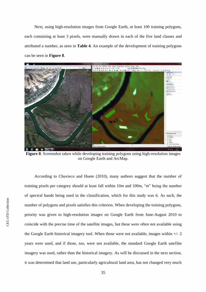
CE

UeT

DC

olle

ctio

n

35

Next, using high-resolution images from Google Earth, at least 100 training polygons,

each containing at least 3 pixels, were manually drawn in each of the five land classes and

attributed a number, as seen in Table 4. An example of the development of training polygons

can be seen in Figure 8.

Figure 8. Screenshot taken while developing training polygons using high-resolution images

on Google Earth and ArcMap.

According to Chuvieco and Huete (2010), many authors suggest that the number of

training pixels per category should at least fall within 10m and 100m, ―m‖ being the number

of spectral bands being used in the classification, which for this study was 6. As such, the

number of polygons and pixels satisfies this criterion. When developing the training polygons,

priority was given to high-resolution images on Google Earth from June-August 2010 to

coincide with the precise time of the satellite images, but these were often not available using

the Google Earth historical imagery tool. When those were not available, images within +/- 2

years were used, and if those, too, were not available, the standard Google Earth satellite

imagery was used, rather than the historical imagery. As will be discussed in the next section,

it was determined that land use, particularly agricultural land area, has not changed very much

CE

UeT

DC

olle

ctio

n

36

over time. As such, using satellite images that are not from the exact time period under study

was deemed adequate. While the trainings were predominantly based on the Google Earth

satellite images, it was helpful to compare the two different Landsat tile dates in ArcMap to

determine the accurate identification of certain classes, e.g. agriculture. For agricultural fields

that are in use, the spectral signature is different in June than it is in August, when, for

example, fields are covered in crops and then later harvested, as seen in Figure 9. The ability

to see these dynamics on the Landsat tiles aided in the proper identification of existing

agricultural lands, versus fallow fields.

Date 1 Date 2

Figure 9. Comparison of spectral signatures of agricultural land in June versus August.

(USGS 2014).

Classification

There are a number of classification algorithms, both traditional and advanced, for land

use land cover classification (Lu and Weng 2007). These algorithms vary in complexity,

accuracy, and computational time and fall into two categories 1) supervised and 2)

unsupervised. Supervised classification assumes some existing knowledge of the study area,

which the user can utilize to determine the most appropriate land use classes. Unsupervised

classification implies no previous knowledge of the area and instead relies on the

classification algorithm to determine clusters of homogenous spectral characteristics, which

the user will categorize and define later (Chuvieco and Huete 2010). While supervised

CE

UeT

DC

olle

ctio

n

37

classification is often preferred for land use classification (Heinl et al. 2009), both types have

been found to be successful when used either alone or in combination (Rozenstein and

Karnieli 2011). The most widely used and well-known supervised algorithm (Chuvieco and

Huete 2010; Otukei and Blaschke 2010), is called the maximum likelihood classification

(MLC) and is what will be utilized in this study. Maximum likelihood is one of the traditional

classification algorithms that is based on statistical probabilities and that relies upon an

assumption of normally distributed data, which remote sensing data often satisfies (Chuvieco

and Huete 2010).

GRASS GIS was used to perform the classification, but in order to do so, the data had to

be prepared in a certain way. The Landsat mosaics were imported into GRASS and grouped

together into one file using the GRASS command [i.group]. The resulting file contained 12

layers (2 mosaics, 6 bands each). The training files (5 in total, one for each class) were

merged together into one file that noted the numeric value of their land use class, as noted in

Table 4, and then imported into GRASS and converted from vector file type to the required

raster file format. Next the command [i.gensig] was run to develop what GRASS calls

―signatures‖ (their term for ―trainings‖). The MLC was then run using GRASS [i.maxlik]

with the following inputs: 1) Group: combined Landsat mosaics, 2) Subgroup: combined

Landsat mosaics, 3) Sigfile: the signatures that had been developed with the training files, 4)

Class: the name of the output file, which will contain the results of the MLC. The

classification took approximately one hour, which produced a file that could be exported to

raster format and then imported into ArcMap for viewing. The classification output, seen in

Figure 10, exhibited an obvious delineation between the two right-hand and two left-hand

tiles, a result of the tiles being from different dates and not generating ample training

polygons in these two tiles to highlight the variation in spectral signatures among the tiles and

dates for each of the five classes.

CE

UeT

DC

olle

ctio

n

38

Figure 10. First (and unsuccessful) MLC output viewed in ArcMap. (Map created by author).

As discussed in the previous section, the last step in the classification process typically

includes repeat iterations to improve the classification and resulting accuracy, which is done

after the validation and accuracy assessment have been completed, which had not yet been

done for this research. But since the problem was fairly obvious, it was decided to return to

the training development without performing these other two steps first, knowing that the

accuracy would be quite low. More polygons were developed, primarily in the left-hand two

tiles, for each of the five classes. The total number of polygons and pixels for this second (and

final) attempt can be found in Table 5. As illustrated in the table, the number of pixels per

class is above and beyond the aforementioned requirement of at least 10m to 100m.

CE

UeT

DC

olle

ctio

n

39

# Class Polygons Pixels

1 Agriculture 215 149,110

2 Forests 129 2,150

3 Grasslands 206 5,482

4 Other 139 1,452

5 Water 183 98,655

Table 5. Number of polygon trainings and pixels developed for the second classification.

After these additional trainings were developed, the MLC was run again using the

aforementioned process in GRASS GIS. The classification output from the second attempt

can be seen in Figure 11.

Figure 11. Second (and final) MLC output viewed in ArcMap. (Map created by author).

CE

UeT

DC

olle

ctio

n

40

Unlike the first output, the second MLC output didn‘t exhibit the sharp delineation

between tiles. There is a slight line (in grey, part of the ―other‖ category) visible due to the

mosaicking process and the rough edges on the Landsat tiles, but it did not end up impacting

the integrity of the classification accuracy, which is discussed in the next section.

Accuracy Assessment

Due to the inherent complexity of classification, it is recommended that an accuracy

assessment be performed in order to evaluate the accuracy of the classification output to a

higher and more reliable degree than mere visual assessment (Congalton 1991). Accuracy

assessment encompasses sampling, validation, and development of accuracy statistics.

Sampling

The two most common types of sampling methods for land use classification accuracy

assessment are simple random sampling and stratified random sampling. Stratified random

sampling ensures that a minimum number of samples are chosen from each ―strata‖ or, in this

case, land use classes. Since there are some classes representing small areas (e.g. the ―other‖

category that includes barren land and impervious surfaces), this method was chosen so these

categories would not be underrepresented as they would likely be with simple random

sampling (Congalton 1991). According to Congalton (1991), for large areas of land

encompassing more than one million acres (approximately 4,000 km2), which is true of the

study area, at least 75 or 100 samples should be chosen per land use class. The number of

samples for each land use class can be altered if there are classes of particular interest or

importance to the classification objectives (Congalton 1991). In accordance with Congalton

(1991), a total of 200 samples were generated for the agriculture class, which is of particular

interest to the classification because it will be tied to agricultural statistics and thus should be

ensured that the classification is done with a higher rate of accuracy. A total of 400 samples

CE

UeT

DC

olle

ctio

n

41

were generated for the four non-agriculture classes, totalling 600 points overall, yielding at

least 100 points per class.

The samples were developed by generating random points using GRASS GIS command

[r.mask]. The ―mask‖ function was used to select only the agriculture class, for which 200

points were allocated, and then used again to select non-agricultural classes, for which 400

points were allocated. These points were exported in vector file format and imported into

ArcMap and then converted into KML file format to be used concurrently in Google Earth.

Figure 12 shows the random points that were generated, blue for the agriculture class, yellow

for the non-agricultural classes.

Figure 12. 600 random points used for classification validation. (Map created by author).

CE

UeT

DC

olle

ctio

n

42

Validation

The next step included scrutinizing each individual sample (random point) using high-

resolution images on Google Earth and the Landsat satellite images in ArcMap to determine

which land use land cover class it belonged to. See Figure 13 and Figure 14 for a visual

representation of this process.

Figure 13. Screenshot taken while conducting random point validation using Google Earth

and ArcMap.

Figure 14. Screenshot taken of a zoomed in representation of random point validation using

Google Earth and ArcMap.

CE

UeT

DC

olle

ctio

n

43

For each individual point, the actual land cover class was documented (using the

numerical categories in Table 4) in the attribute table of the random points GIS shapefile.

Points that were either too close to borders to ascertain what the proper land class was were

given the value 999. Those that were obscured by minor cloud cover were given 444. Points

that appeared close together were measured to ensure they were at least 500 m apart so as not

to have samples that were too close to each other. The total number of points per class that

were sampled is found in Table 6. The validated sample files were merged together with

QGIS, excluding the points identified as ‗444‘ or ‗999‘, for a total of 532 sample points, still

greater than the recommended 100 points per class.

Category Class or Description Number

1 Agriculture 189

2 Forests 25

3 Grasslands 250

4 Other 11

5 Water 57

444 Obscured by clouds 5

999 Border, cannot confidently determine 63

Table 6. Points per class sampled in the classification process.

Assessment

To determine accuracy statistics for the land use land cover classification, a Kappa

Analysis was performed using GRASS GIS command [r.kappa]. This analysis provides

overall accuracy statistics, an error matrix, and the Kappa statistic. The use of an error matrix

is the most common way to represent accuracy statistics resulting from classification

(Congalton 1991; Foody 2002). The output from the accuracy assessment including all of

these parameters is shown in Figure 15. The desired overall accuracy for land use land cover

classification is at least 85% (Thomlinson et al. 1999).

CE

UeT

DC

olle

ctio

n

44

Class 1

(Agriculture)

Class 2

(Forested)

Class 3

(Grasslands)

Class 4

(Other)

Class 5

(Water) Total

Class 1 178 0 6 0 0 184

Class 2 0 25 1 0 0 26

Class 3 10 0 241 0 0 251

Class 4 1 0 2 11 2 16

Class 5 0 0 0 0 55 55

Total 189 25 250 11 57 532

Commission Omission Estimated Kappa

Class 1 (Agriculture) 3.26% 5.82% 0.95

Class 2 (Forested) 3.85% - 0.96

Class 3 (Grasslands) 3.98% 3.60% 0.92

Class 4 (Other) 31.25% - 0.68

Class 5 (Water) - 3.51 1.00

Figure 15. Kappa analysis output: error matrix.

The error matrix in Figure 15 shows the classification output in rows and validated

points in columns. The bolded numbers going diagonally show the number of points the

classifier classified correctly for each class. As an example, in the first row, the classifier

correctly classified 178 points in the agriculture class, but it also classified 6 points as

agriculture that were actually in the grasslands class. These data are summarized in the

commission (errors of inclusion) and omission statistics (errors of exclusion) in Figure 15

(Congalton 1991). For Class 1 (Agriculture), the commission error is 6 / 184 = 3.26%. There

were 6 points that were incorrectly included in the agricultural class, but that were actually

grasslands. And the omission error for Class 1 is 11 / 189 = 5.82%. There were 10 points the

classifier thought were grasslands and 1 point the classifier thought was in the ―other‖ class

that were actually agriculture, so these points were incorrectly excluded. The commission

error for Class 4 (Other) is higher than the others, but this class represents a very small

portion of the study area and did not greatly impact the overall accuracy for the classification.

The overall accuracy was 95.86%, calculated by the total correct observations (510)

divided by the total observations (532). The Kappa statistic was 0.94, also indicating the

suitability of the classification. The Kappa statistic is a well-known and utilized parameter in

CE

UeT

DC

olle

ctio

n

45

accuracy assessment of land use classification (Otukei and Blaschke 2010; Heinl et al. 2009;

Abd El-Kawy et al. 2011; Rozenstein and Karnieli 2011). It takes into consideration pixels

that have been properly classified due to random chance rather than proper classification

(Chuvieco and Huete 2010; Foody 2002) and is a metric of the accuracy and suitability of the

classification output. A value of 1 is perfect, so the obtained value of 0.94 is very good.

Result of Classification

Because the desired level of accuracy was exceeded for the classification, no repeat

iterations were deemed necessary. To calculate proportional land use class statistics, raster

statistics were calculated using the ―Build Raster Attribute Table‖ tool in ArcMap. Within the

study area, the classification found the following proportions for each land class: 57.0%

Agriculture, 3.1% Forested, 31.3% Grasslands, 2.8% Other, and 5.7% Water. The next step

was to transform the classification output into a thematic land use map, which is described in

the next subsection.

4.1.2. Development of a Land Use Thematic Map

Since the land use classification accuracy was found to be adequate, this information

was used to generate a final thematic map showing land use in the study area using ArcGIS.

The map was originally created using the 80 km buffer zone around the entire reservoir. If the

map were to be used in actual runoff modelling, a modified buffer zone can easily be applied,

as was done as an example in the final map. When used in runoff modelling, there is a low

likelihood that runoff from below the reservoir would make its way up to it. This does remain

a possibility, due to the constant back-and-forth movement of water at the base of the

reservoir from transportation and shipping, but its effects are not likely significant. As such, a

modified buffer zone was applied to the final map, which can be seen in Figure 21.

CE

UeT

DC

olle

ctio

n

46

4.1.3. Determination of Agricultural Land Use Change

The last step in addressing RQ1 is to examine how land use has changed in the region in

recent years. Since the land use of interest is agricultural land (cropland), statistics were

obtained from the Russian Federal Service of State Statistics providing the total area of

croplands from 1995 to 2009 (statistics from 2010 were not available) in the Rostov and

Volgograd oblasts, which can be seen in Appendix Figure 3 (ROSSTAT 2010).This data was

compared to the total land area of each region (National Census 2014) to determine the

percentage of agricultural lands within each oblast for the period, as seen in Figure 16.

Figure 16. Cropland as a percentage of total land area, 1995 to 2009. Data source:

(ROSSTAT 2010)

As seen in Figure 16, the proportion of cropland in both Rostov and Volgograd oblasts

has stayed relatively constant since 1995. It must be noted that these statistics are at the oblast

level, and are thus representing a larger area than the area under study (80 km around the

reservoir). But because there has not been much change overall and because the land use

classification determined agricultural lands constituted approximately 57.0% of the total study

area, this data is assumed to be representative of the study area.

CE

UeT

DC

olle

ctio

n

47

Another indication of the use of agricultural lands is through crop yield data. Crop yield

statistics were obtained for a number of area crops, also from the Russian Federal Service of

State Statistics, at the oblast level, for the period between 1995 to 2009 (ROSSTAT 2010).

During this time, grain and forage crops have made up a substantial amount (ranging from 70-

80%) of the sown area in these two regions, as seen in Figure 17. Because of the dominance

of grain and forage crops in the area, yields from these crops were investigated.

Figure 17. Grain and forage crops as the predominant crops in the region. Data source:

(ROSSTAT 2010)

Crop yield data was obtained at the oblast level for 9 grain and forage crops: annual

grass hay, barley, grain, oats, perennial grass hay, spring wheat, winter wheat, and sugar

beets. Crop yields for the first 8 crop types are shown in Figure 18 for Volgograd and Figure

19 for Rostov. Sugar beets were graphed separately in Figure 20 because the yield is

measured in quintals per hectare, which is a value of mass. Sugar beets have a higher mass

than other grain and forage crops, e.g. winter wheat, and are more easily viewed with a

different vertical axis.

While there is apparent fluctuation of the crop yields for the period and an overall

increase in a few of the crops‘ yields (e.g. grain and winter wheat), some of the crop yields

CE

UeT

DC

olle

ctio

n

48

remained relatively constant for the period. Crop yields can fluctuate on a yearly basis based

on the climatic and meteorological conditions, as well as on the application of and timing of

fertilizers. In order to make a conclusion on the crop yields and their potential effect on

agricultural land use, more information, e.g. fertilizer application statistics, would need to be

obtained for the entire region, which was not available at the time of research.

Figure 18. Volgograd grain and forage crop yields (excluding sugar beets) from 1995 to

2009. Data source: (ROSSTAT 2010)

Figure 19. Rostov grain and forage crop yields (excluding sugar beets) from 1995 to 2009.

Data source: (ROSSTAT 2010)

CE

UeT

DC

olle

ctio

n

49

Figure 20. Sugar beet yields for both oblasts from 1995 to 2009. Data source: (ROSSTAT

2010)

4.1.4. Summarizing Work Conducted for RQ1

The aforementioned work and analysis has answered the first research question and has

produced a valuable deliverable, which can be used for future research. A land use

classification was performed for the study area, finding 57.0% of the region to be comprised

of agricultural lands. A thematic land use map has been developed (Figure 21), which

provides a basis for future land use studies and can be used as a base for future studies of land

use change in the region. It was also determined that the proportion of agricultural lands has

not changed much over the period of study.

CE

UeT

DC

olle

ctio

n

50

Figure 21. Final land use map. (Map created by author).

4.2. Analysis of Eutrophic Algal Blooms (RQ2)

The second research question aims at determining when algal bloom events have

occurred and to what extent they have occurred in the past 15 years. Another goal is to

develop a list and a visual catalogue of all eutrophic algal blooms that have been identified

through satellite imagery and publish these findings online.

4.2.1. Identification of Eutrophication Events

The first step in answering the second research question is to identify instances of algal

blooms in the reservoir. As discussed before, because of the quality and consistency of the

CE

UeT

DC

olle

ctio

n

51

Landsat program, the U.S. Geological Survey database will again be used to obtain satellite

imagery. As was noted in Section 3, algal blooms are easy to identify on satellite images and

thus this method of browsing the available satellite images in the Landsat database was

deemed sufficient. Three of the four tiles, Path/Row 173/027, 173/026, and 172/027 as seen in

Figure 5, were used for this part of the research, as tile 172/026 covered a only small portion

of the reservoir in comparison to the other three. More than one tile was used because tiles

often have images from different dates, so using more than one tile increases the number of

dates available for analysis.

Each individual satellite image for the three tiles from May to October between 1990

and 2013 was studied on the USGS database website (www.glovis.usgs.gov) at 240 m

resolution to identify algal blooms. Since the goal of this research is to determine agricultural-

related causes, other months in the year that fell outside of the agricultural season were

excluded. Each image that demonstrated an algal bloom event (large or small) was

downloaded and recorded. This catalogue of images and their corresponding dates can be

found in Appendix Figure 4 and has been published online at the Azov Center website at

http://azovcenter.ru/tsimlyansk-algal, as can be seen in Appendix Figure 5.

Unlike the land use classification application of the Landsat tiles, factors like cloud

cover, satellite type, and quality were not of concern for this part of the study, as the tiles were

not used in software applications, only for visual examination. If eutrophication could easily

be identified through clouds obscuring the image, the tile was still used. Tiles from the

Landsat 7 mission (post 2003 scanner malfunction) were also included, as eutrophic algal

blooms were still easily identifiable beyond the missing scan lines.

The availability and ability to download Landsat images was also mentioned in Section

3. This, too, was not a concern for this part of the research. The land use classification

required a special specific file type, called the ―Level 1 Product‖, which contains all 7 spectral

CE

UeT

DC

olle

ctio

n

52

bands. These comprehensive files are often not available for download. But for every image

that can be seen on the USGS database, a simple preview image can be downloaded, called

the ―LandsatLook ‗Natural Color‘ Image‖. These images were sufficient for the algal bloom

existence and extent analysis. A total of 82 images showing algal blooms were collected.

Images from the same date but on different tiles were not repeated and the tile exhibiting the

larger extent of the bloom was selected.

4.2.2. Determination of the Extent of Identified Algal Blooms

Next, each image was scrutinized to determine the extent of the algal bloom in the

reservoir. For each image, the bloom concentration was deemed ―Minor‖, ―Moderate‖, or

―Extensive‖ based on the appearance of the bloom. The size of the algal bloom in the

reservoir was deemed ―Small‖, ―Medium‖, or ―Large‖. After determining these two

qualitative parameters, the extent was determined to be ―Low‖, ―Medium‖ or ―High‖, based

on the criteria in Table 7, with a corresponding numerical level, which will be used in the

next section.

Determined Extent Bloom Concentration Bloom Size

High (Level 3) Extensive Large

Medium (Level 2) Moderate Medium or Large

Low (Level 1) Small Small or Medium

Table 7. Algal bloom extent criteria.

While this process could have been done in a more quantifiable way, e.g. drawing a

polygon around the area of the reservoir in ArcGIS and calculating the area or proportion to

the reservoir, the size of the bloom is only one factor. Concentration is another major factor.

Having a scale based purely on size would not be representative of the actual state of the

bloom, as a large bloom with low concentration could show to be of a higher extent than a

medium-sized bloom with a very high concentration. As such, these factors were taken into

consideration when making a qualitative assessment of the extent of the bloom.

CE

UeT

DC

olle

ctio

n

53

A total of 17 dates were determined to have a ―High‖ (Level 3) algal bloom extent.

These 17 images can be seen below in Table 8. A ―Low‖ (Level 1) algal bloom was identified

on 42 dates, and ―Medium‖ (Level 2) was identified on 23 dates. The full table of all

identified algal blooms is at Appendix Figure 4, which was also published online at http://

http://azovcenter.ru/tsimlyansk-algal.

#3, 172/027, 9 Sept. 1990 #5, 172/027, 11 October 1990 #6, 173/027 18 August 1991

#7, 173/027, 19 Sept. 1991

#18, 173/027, 19 Sept. 1997

#29, 173/027, 20 Sept. 2003

#30, 172/027, 15 October 2003

#33, 172/027, 7 Sept. 2004

#34, 173/027, 14 Sept. 2004

CE

UeT

DC

olle

ctio

n

54

#40, 172/027, 13 Sept. 2006

#42, 172/027, 7 October 2006

#49, 172/027, 2 Sept. 2008

#54, 173/027, 19 August 2009

#56, 172/027, 29 Sept. 2009

#69, 173/027, 12 Sept. 2012

#74, 173/027, 27 June 2013

#81, 173/027, 1 October 2013

Table 8.Satellite-identified algal blooms with a "High" bloom extent.

The temporal distribution of identified algal blooms from the satellite images is found

by month in Table 9. Based on the blooms identified through the satellite images, most algal

blooms occur within August and September. This is consistent with literature, discussed in

Section 2, which says that a large bloom often occurs in late summer. In Section 1 of this

study, a number of environmental events (e.g. fish kills) were mentioned resulting from algal

CE

UeT

DC

olle

ctio

n

55

blooms in recent years (2007-2001). As has been shown through this research, these algal

blooms are not a recent phenomenon. They have been occurring on an almost yearly basis

(from what can be ascertained through the available satellite images) in varying degrees since

at least 1990.

Month Number of

Images

Percent of

Total

June 4 4.9%

July 14 17.1%

August 22 26.8%

September 26 31.7%

October 16 19.5%

Table 9. Temporal distribution (by month) of identified algal blooms.

After these blooms were identified, other data sources were explored for identifying

additional algal bloom events, including NASA‘s Ocean Color portal

(oceancolor.gsfc.nasa.gov). Using the Level 3 Browser, every date in which a ―High‖ algal

bloom occurred was searched for using the Aqua MODIS Chlorophyll concentration option to

see if the two sources would match, which would mean that this source could be used as

another tool to identify additional algal blooms. But only 2 of the 17 dates (7 September 2004

and 29 September 2009) showed any sign of chlorophyll, presumably because the very coarse

resolution, as seen in Figure 22. The Tsimlyansk Reservoir can be seen in the middle of the

image between the Black Sea and Caspian Sea and a very small amount of red can be

identified within the reservoir indicating a high concentration of chlorophyll-a, an indicator of

cyanobacteria (Tebbs, Remedios, and Harper 2013), which is noted as one of the main types

of algae associated with algal blooms in the reservoir in Section 2. Due to the apparent

superiority of using the Landsat database to identify algal blooms because of the better

resolution, this source was not used to search for other algal bloom events. No other data

source provided adequate identification of blooms and as such, the data obtained from the

Landsat database were relied upon for study.

CE

UeT

DC

olle

ctio

n

56

Figure 22. Screenshot from the NASA Ocean Color Level 3 Browser. Image from: (NASA

2014)

4.2.3. Summarizing Work Conducted for RQ2

The second research question (RQ2) was fulfilled by the aforementioned research. A total

of 82 algal bloom events were identified through the use of satellite imagery, including 17

events whose extent was deemed ―High‖ (Level 3). From the information gathered, it is clear

that algal blooms of varying degrees have been occurring on an almost yearly basis since

1990 and are not a recent phenomenon.

Pursuant to the research question, a catalogue of all the algal bloom events found in the

USGS database was developed, including an assessment of the extent of the bloom. The

catalogue of images and their corresponding dates can be found in Appendix Figure 4 and

the list of algal bloom events with the determination of the bloom extent can be found in

Appendix Figure 6. The next step, which appears in the following section, will be to see if

there is a relationship between land use and these eutrophication events.

CE

UeT

DC

olle

ctio

n

57

4.3. Finding Relationships (RQ3)

Now that the first two research questions relating to land use and algal bloom events have

been addressed and concrete deliverables have been developed, the next step is to explore an

example how this data can be used to begin to understand the relationship between land use

and eutrophication in the reservoir. The two components will be investigated through the use

of precipitation data, one of the factors involved in the development of algal blooms, to see if

a relationship can be identified.

4.3.1. Investigation into Precipitation-Induced Algal Blooms

The objective aims to investigate the relationship between land use and algal blooms

through precipitation. Precipitation events can stimulate the movement of agricultural runoff,

including nitrogen- and phosphorus-based fertilizers, into water bodies (Reichwaldt and

Ghadouani 2012; Chorus and Mur 1999; Spatharis et al. 2007; Heisler et al. 2008; Glandon et

al. 1981).

To investigate this in the Tsimlyansk Reservoir, precipitation data for the region

surrounding the reservoir was obtained from the Giovanni web portal, which was discussed in

Section 2. The Meteorological Portal, TRMM Online Visualization and Analysis System

(TOVAS) was used to obtain daily rainfall estimates for the area: West 41.438, North 49.975,

South 46.375, and East 44.306, ensuring full enclosure of the reservoir and buffer zone, as

seen in Figure 23.

CE

UeT

DC

olle

ctio

n

58

Figure 23. Screenshot showing the geographical extent of Giovanni precipitation data. Image

from: (NASA 2013a)

Daily rainfall data was obtained for every year available on the Giovanni portal (1998 to

2013, slightly different than the time frame for land use and eutrophication research, but still

covering a 15 year period) for the period of May to October, to match the time period for the

identification of algal blooms. Using Microsoft Excel, a graph of precipitation for the period

was generated for each year. The algal bloom event data developed in the previous section

was added to each precipitation graph on a second vertical axis. As with the scale that had

been developed, ―High‖ instances are indicated by a 3, ―Medium‖ by a 2, and ―Low‖ by a 1.

While the specific vertical placement of the algal bloom events on the graph is arbitrary, it

clearly identifies when the satellite-identified bloom occurred and of what magnitude it was.

For certain years, there appears to be a clear relationship between precipitation and algal

bloom events, as seen in Figure 24. In 2003, the three largest rainfall events occurred on 11

August (15.586 mm), 4 September (12.959 mm), and 11 October (19.007 mm). Similarly, one

medium and two large algal blooms were identified through the satellite images, each

occurring a shortly after each rainfall event on 28 August, 20 September, and 15 October,

respectively, indicating a relationship.

CE

UeT

DC

olle

ctio

n

59

Figure 24. Precipitation vs. algal blooms for 2003. Data source: (NASA 2013a; USGS 2014)

A number of other years show similar patterns, e.g. 2000 and 2001 seen in Figure 25

and Figure 26, respectively. Two algal blooms were identified in 2000, both occurring shortly

after episodes of rain occurring a multiple days within a short period of time. The three algal

blooms that were identified in 2001 all occurred amidst periods of rain as well.

Figure 25. Precipitation vs. algal blooms for 2000. Data source: (NASA 2013a; USGS 2014)

CE

UeT

DC

olle

ctio

n

60

Figure 26. Precipitation vs. algal blooms for 2001. Data source: (NASA 2013a; USGS 2014)

There does appear to be a relationship between precipitation and algal blooms based on

these images, but in other years studied, the relationship wasn‘t as clear. An example of this is

in 2012, when a number of algal bloom events occurred, some of them deemed ―High‖ and

―Medium‖, yet precipitation remained relatively low over the time period. This graphs is seen

in Figure 27. All of the graphs used for analysis, from 1998 to 2013 can be found in

Appendix Figure 7.

Figure 27. Precipitation vs. algal blooms for 2012. Data source: (NASA 2013a; USGS 2014)

CE

UeT

DC

olle

ctio

n

61

4.3.2. Summarizing Work Conducted for RQ3

The aforementioned work and analysis has addressed the objective of RQ3. An example

of how the developed land use and eutrophication data can be utilized was investigated.

Through the lens of precipitation, it was determined that there is a potential relationship

between the two components, although more work can be done to further investigate each

event and identify more events to solidify the presumed relationship between the two.

But the applicability of the developed land use and eutrophication data is clear. Using

these two remote sensing- and GIS-derived components, other variables (e.g. precipitation

data) can be added to study potential causal relationships between these two elements.

CE

UeT

DC

olle

ctio

n

62

5. Discussion

5.1. Research Results and Limitations

A primary aim of this study was to conduct the preliminary groundwork for future

research and to generate a set of deliverables that can be used and expanded upon in the

future. In addition, another main goal was to make use of remote sensing and GIS

technologies as well as to explore and utilize the vast amount of data available through data

portals. These overall aims were pursued through the lens of three research questions, targeted

at investigating potential agricultural-related causes of eutrophication in the Tsimlyansk

Reservoir. The following section will discuss the results of the work conducted for each of

these research questions as well as their limitations.

5.1.1. Land Use Classification

Regarding the first research question, the land use classification that was performed was

determined to have an overall accuracy of 95.86%, deeming it a suitably accurate

representation of land cover in the area surrounding the reservoir in 2010. The land use map

resulting from this process can be used as a foundation for further research in both land and

water applications, similar to how it was used in this study to investigate the relationship

between land use and eutrophication through precipitation.

While the desired classification accuracy was achieved (and exceeded), there are some

factors to take into consideration when relying upon digitally classified data. Although the use

of digital classification of remote sensing images to develop land use thematic maps is very

common, there are a number of constraints and limitations associated with it. The most

notable limitation is due to the inherent subjectivity involved throughout the entire process: 1)

interpreting both high-resolution images and Landsat satellite imagery, 2) developing the

CE

UeT

DC

olle

ctio

n

63

training areas, 3) validating the random sampling points, and 4) interpreting the accuracy

statistics. Human subjectivity and human error play a role in this process, which inevitably

impact the true accuracy of the classification output and resulting thematic map. To overcome

this, additional sources of information are often used in land classification studies, including

actual ground-truth data acquisition, which is physically visiting the study area to ascertain

the proper land class at specific points. But this, too, involves some degree of subjectivity on

the part of the individual conducting the ground-truthing (Prishchepov 2014). Because of

feasibility issues, physical ground-truthing was not conducted for this study and classification

instead relied upon the interpretation of high-resolution images and Landsat satellite images

as reference data. Taking this into consideration, the land use classification developed still

provides a sound basis for future research in the area.

5.1.2. Land Use Change

The statistics obtained to determine how agricultural land has changed over the past 15

years were at the oblast level. These statistics represent an area larger than the buffer zone for

which the land use classification was developed, based on the approximate potential travel

distance of phosphorus in agricultural runoff. Obtaining statistics for the particular rayons (the

next smallest administrative level) that fall within the buffer zone would yield more accurate

results regarding the actual changes in agricultural land in the immediate vicinity around the

reservoir. But since the results showed that the proportion of agricultural land has remained

relatively stable over the time period studied, these results were assumed to be representative

of the smaller area.

5.1.3. Land Use Map

The final map developed in Section 4.1 (Figure 21) used a modified buffer zone for the

purposes of taking into consideration the low likelihood of runoff from below the reservoir

CE

UeT

DC

olle

ctio

n

64

travelling upwards to the reservoir. Depending on the intended use of the classified land use

map (e.g. for uses in modelling), other approaches could be taken to modify this buffer zone,

e.g. based on a drainage basin for the reservoir or based on a digital elevation model of the

area.

5.1.4. Identification of Algal Blooms

A total of 82 algal blooms were identified through Landsat satellite imagery from 1990-

2013. Having identified these bloom occurrences, additional work could be done to examine

each individual event to attempt to identify the underlying cause or set of factors.

While the identification of algal blooms through satellite imagery was achieved, the

images (and corresponding dates) identified do not represent all of the algal blooms that

occurred in the time period, due to the limited temporal availability of Landsat imagery. Only

blooms that occurred on 1) dates for which images were taken and 2) images in which an

algal bloom could still be identified through atmospheric interference were identified. Years

in which there were an absence of images does not necessarily indicate an absence of bloom

activity. To address this, more remote sensing data sources could be investigated to find

additional dates showing algal blooms. Additionally, other sources of information, like

additional news articles, could be investigated to make the sample more representative of

actuality. But this aside, the identified algal blooms do present a viable set of information that

can be used as a basis for further research.

5.1.5. Comparing Land Use and Algal Blooms Through Precipitation

A relationship between precipitation and algal blooms was indeed identified and is very

evident in a few of the years under study (e.g. 2000, 2001, and 2003). But as the set of

satellite imagery used to identify these blooms is not representative of all the algal blooms

CE

UeT

DC

olle

ctio

n

65

that have occurred during the study period, more information would have to be obtained to

conclude on a causal link between the two.

5.2. Pathways for Further Research

The work done for this research has set a foundation for future research to be able to be

conducted in the region around the reservoir. More factors can be investigated and combined

with the existing findings to strengthen the existence of potential causal relationships (e.g.

between precipitation and algal blooms, as was explored through this research) and to identify

new relationships. Future research could include 1) investigating the role air temperature

plays in the development of algal blooms; 2) obtaining data on the specific time, amount, and

composition of fertilizer applications (ideally on a field-by-field basis); 3) combining both of

these factors with the developed precipitation data to see what combination of factors causes

blooms to occur (e.g. a few days of hot temperatures around the time of a fertilizer

application, followed by a large precipitation event). Combining these and other

environmental factors with the results obtained through this research could lead to further

discoveries about the underlying causes of algal blooms and get closer to finding ways to

mitigate the effects of future occurrences. In addition, further research could involve finding

new sources of satellite imagery to identify additional algal blooms or finding and applying

new ICTs.

Overall, the research conducted for this study provides a fundamental basis for future

work to be done in the region and provides an example of how data portals, remote sensing

and GIS can be used to apply to environmental issues. There are a number of pathways for

future research that would involve combining new factors with the results already obtained to

gain further understanding of the underlying causes of eutrophication in the Tsimlyansk

Reservoir and get closer to identifying ways to mitigate the effects of harmful algal blooms,

thereby addressing one of the facets of water security in the region.

CE

UeT

DC

olle

ctio

n

66

6. Conclusion

The overall goals of this research were to conduct the preliminary groundwork and

develop deliverables (e.g. catalogue of algal blooms) for future research in the region; make

use of the immense amount of data that is currently underutilized; and provide an example of

how remote sensing and GIS technologies can be applied in a practical and useful manner.

These general goals were addressed through the use of three research questions aimed at

investigating potential agricultural-related causes of eutrophication in the Tsimlyansk

Reservoir, an issue that has been causing problems and threatening water security in the

region in recent years:

RQ1: What was the state of land use around the Tsimlyansk Reservoir around the time

of reported harmful algal blooms? Has it changed much over the past 15 years?

RQ2: When and to what extent have algal blooms occurred in the Tsimlyansk Reservoir

in the past 15 years?

RQ3: How can this data be used to investigate the relationship between land use and

eutrophication in the Tsimlyansk Reservoir?

To address the first research question, a land use classification was performed using

remote sensing and GIS data and technologies, which yielded a detailed functional land use

map of the study area in 2010. The map that was developed can be used as a basis for future

research in the region and can easily be modified based on its intended function. It was

determined that the proportion of agricultural land use in the region has remained relatively

stable over the past 15 years, therefore pointing to other more complex factors as potential

sources of eutrophication in the reservoir.

The second research question was answered by obtaining and evaluating satellite imagery

exhibiting algal blooms in the reservoir. A catalogue of this information was developed and

made publicly available at http://azovcenter.ru/tsimlyansk-algal for interested stakeholders.

CE

UeT

DC

olle

ctio

n

67

As identified through satellite imagery, algal blooms of varying extents (low, medium, and

high) have occurred on an almost yearly basis since 1990 and are not a new phenomenon.

The third research question aimed to provide an example of how the data obtained and

developed through the use of data portals and remote sensing and GIS technologies can be

used to identify relationships between the two components. Land use and eutrophication were

investigated through the lens of precipitation, ultimately discovering a relationship between

the two. More work can be done to gather more information about each algal bloom identified

and to identify a larger sample to solidify the presumed relationship between the two

elements.

The three research questions were answered and the goal of developing the fundamental

groundwork for future research was achieved. Furthermore, data has been obtained and made

accessible to be a valuable and time-saving resource for interested stakeholders wanting to

continue research of land use and eutrophication in the region. These deliverables are already

accessible and can be found at www.azovcenter.ru/tsimlyansk-algal and

www.azovcenter.ru/tsimlyansk-landsat. And lastly, this research set out to make use of the

continually expanding set of available ICTs and vast amount of data freely available through

data portals and apply these to a practical environmental problem. This aim was achieved by

sorting through and collecting data from remote sensing data portals and utilizing this data in

conjunction with multiple remote sensing and GIS techniques in a novel way.

CE

UeT

DC

olle

ctio

n

68

References

Abd El-Kawy, O. R., Rød, J. K., Ismail, H. A., and Suliman, A. S. 2011. Land use and aand

cover change detection in the Western Nile Delta of Egypt using remote sensing data.

Applied Geography 31 (2): 483–94.

Agarwal, A., delos Angeles, M. S., Bhatia, R., Chéret, I., Davila-Poblete, S., Falkenmark, M.,

Vilarreal, F. G., Jønch-Clausen, T., Kadi, M. A., Kindler, J., Rees, J., Roberts, P.,

Rogers, P., Solanes, M., Wright, A. 2000. Integrated Water Resources Management:

Global Water Partnership Technical Advisory Committee. Stockholm: Global Water

Partnership.

American Farmland Trust. 2013. Controlling nutrient runoff on farms.

Barnes, B. B., Hu, C., Holekamp, K. L., Blonski, S., Spiering, B. A., Palandro, D. and

Lapointe, B. 2014. Use of Landsat data to track historical water quality changes in

Florida Keys marine environments. Remote Sensing of Environment 140 (January):

485–96.

Brivio, P. A., Giardino, C. and Zilioli, E. 2001. Determination of chlorophyll concentration

changes in Lake Garda using an image-based radiative transfer code for Landsat TM

images. International Journal of Remote Sensing 22 (2): 487–502.

Carpenter, S. R., Caraco, N. F., Correll, D. L., Howarth, R. W., Sharpley, A. N., and Smith,

V. H. 1998. Nonpoint pollution of surface waters with phosphorus and nitrogen.

Ecological Applications 8 (3): 559–68.

Carpenter, S. R., Stanley, E. H., and Zanden, M. J. V. 2011. State of the world‘s freshwater

ecosystems: physical, chemical, and biological changes.‖ Annual Review of

Environment and Resources 36: 75–99.

Chorus, I, and Mur, L. 1999. Preventive measures. In Toxic Cyanobacteria in Water: A Guide

to Their Public Health Consequences, Monitoring and Management, ed. I. Chorus and

E. Bartram. E & FN Spon.

Chuvieco, E., and Huete, A. 2010. Fundamentals of satellite remote sensing. Boca Raton, FL,

USA: CRC Press.

Congalton, R. G. 1991. A review of assessing the accuracy of classifications of remotely

sensed data. Remote Sensing of Environment 37 (1): 35–46.

Elhag, M, Psilovikos, A., and Sakellariou-Makrantonaki, M. 2013. Land use changes and its

impacts on water resources in Nile Delta region using remote sensing techniques.

Environment, Development and Sustainability 15 (5): 1189–1204.

European Union (EU) Directive. 2000. Directive 2000/60/EC of the European Parliament and

of the Council of 23 October 2000 Establishing a Framework for Community Action

in the Field of Water Policy. Accessed April 26. URL: http://eur-lex.europa.eu/legal-

content/EN/TXT/ ?uri=CELEX:32000L0060.

European Union (EU). 2013. ―European Union Open Data Portal.‖ Accessed May 24. URL:

http://open-data.europa.eu/en/data/.

Farag, H., and El-Gamal, A. 2011. Assessment of the eutrophic status of Lake Burullus.

International Journal of Environmental Science and Engineering (IJESE) 2: 61–74.

CE

UeT

DC

olle

ctio

n

69

Ferreira, J. G., Andersen, J. H., Borja, A., Bricker, S. B., Camp, J., Cardoso da Silva, M,

Garcés, E., Heiskanen, A-S., Humborg, C., Ignatiades, L., Lancelot, C., Menesguen,

A., Tett, P., Hoepffner, N., Claussen, U. 2011. Overview of eutrophication indicators

to assess environmental status within the European Marine Strategy Framework

Directive. Estuarine, Coastal and Shelf Science 93 (2): 117–31.

Foody, G. M. 2002. Status of land cover classification accuracy assessment. Remote Sensing

of Environment 80 (1): 185–201.

Gibson, P. J., and Power, C. H. 2000. Introductory Remote Sensing: Principles and Concepts.

London; New York: Routledge.

Gilfanova, I. 2012. Application of SWAT modelling for assessment of ecosystem goods and

services in the Azov Sea basin. Master of Science thesis, Central European University,

Budapest.

Glandon, R. P., Payne, F. C., McNabb, C. D., and Batterson, T. R. 1981. A comparison of

rain-related phosphorus and nitrogen loading from urban, wetland, and agricultural

sources. Water Research 15 (7): 881–87.

GRASS GIS. 2012. "General Overview." GRASS GIS: The World‘s Leading Free GIS

Software. Accessed May 20. URL: http://grass.osgeo.org/documentation/general-

overview/.

Heinl, M., Walde, J., Tappeiner, G., and Tappeiner, U. 2009. Classifiers vs. input variables—

the drivers in image classification for land cover mapping. International Journal of

Applied Earth Observation and Geoinformation 11 (6): 423–30.

Heisler, J., Glibert, P. M., Burkholder, J. M., Anderson, D. M., Cochlan, W., Dennison, W.

C., Dortch, Q., Gobler, C. J., Heil, C. A., Humphries, E., Lewitus, A., Magnien, R.,

Marshall, H. G., Sellner, K., Stockwell, D. A., Stoecker, D. K., Suddleson, M. 2008.

Eutrophication and harmful algal blooms: a scientific consensus. Harmful Algae 8 (1).

HABs and Eutrophication: 3–13.

Kitsiou, D., and Karydis, M. 2011. Coastal marine eutrophication assessment: a review on

data analysis. Environment International 37 (4): 778–801.

Kuemmerle, T., Erb, K., Meyfroidt, P., Müller, D., Verburg, P. H., Estel, S., Haberl, H.,

Hostert, P., Jepsen, M. R., Kastner, T., Levers, C., Lindner, M., Plutzar, C., Verkerk,

P. J., van der Zanden, E. H., Reenberg, A. 2013. Challenges and opportunities in

mapping land use intensity globally. Current Opinion in Environmental Sustainability

5 (5). Human Settlements and Industrial Systems: 484–93.

Kuemmerle, T., Radeloff, V. C., Perzanowski, K., and Hostert, P. 2006. Cross-border

comparison of land cover and landscape pattern in Eastern Europe using a hybrid

classification technique. Remote Sensing of Environment 103 (4): 449–64.

Lagutov, V., and Lagutov, V. 2012. The Azov ecosystem: resources and threats. In

Environmental Security in Watersheds: The Sea of Azov, ed. V. Lagutov, 3–62. NATO

Science for Peace and Security Series C: Environmental Security. Springer

Netherlands.

Lu, D., and Weng, Q. 2007. A survey of image classification methods and techniques for

improving classification performance. International Journal of Remote Sensing 28 (5):

823–70.

CE

UeT

DC

olle

ctio

n

70

NASA. 2013a. ―Giovanni - Interactive Visualization and Analysis.‖ Goddard Earth Sciences

Data and Information Services Center. Accessed May 12. URL: http://disc.sci.

gsfc.nasa.gov/giovanni.

———. 2013b. ―Landsat 8 Launch.‖ NASA. Accessed May 20. URL: http://www.nasa.

gov/mission_pages/landsat/launch/index.html#.U3thfliSzxY.

———. 2014. ―OceanColor Web.‖ Accessed May 22. URL: http://oceancolor.gsfc.nasa.gov/.

National Census. 2002. ―Территория, числорайонов, населѐнныхпунктов и

сельскихадминистрацийпосубъектамРоссийскойФедерации [Territory, number of

districts, inhabited localities, and rural administration by federal subjects of the

Russian Federation]. ВСЕРОССИЙСКАЯ ПЕРЕПИСЬ НАСЕЛЕНИЯ 2002 ГОДА

(National Census 2002). Accessed May 16. URL: http://www.perepis2002.ru/

ct/doc/1_TOM _01_03.xls.

Nikanorov, A. M., Khoruzhaya, T. A., and Martysheva, N. A. 2012. Present-day

characteristics and trends of long-term changes in ecological and toxicological

conditions of the Tsimlyansk Reservoir. Russian Meteorology and Hydrology 37 (4):

269–75.

Nikanorov, A. M., Khoruzhaya, T. A., Minina, L. I., and Martysheva, N. A. 2010. Опасность

«цветения» Цимлянского Водохранилища [Danger of ‗bloom‘ Tsimlyansk

Reservoir]. URL: http://zhurnal.ape.relarn.ru/articles/2010/012.pdf.

Novikova, N. M., Kalioujnaia, I. Y., Kalioujnaia, N. S., Sokhina, E. N., and Zubov, I. A.

2012. Identification and mapping of environmental conflicts for the Tsimlyansk water

reservoir. Arid Ecosystems 2 (3): 156–64.

Oetter, D. R., Cohen, W. B., Berterretche, M., Maiersperger, T. K., and Kennedy, R. E. 2001.

Land cover mapping in an agricultural setting using multiseasonal Thematic Mapper

data. Remote Sensing of Environment 76 (2): 139–55.

Otukei, J. R., and Blaschke, T. 2010. Land cover change assessment using decision trees,

support vector machines and maximum likelihood classification algorithms.

International Journal of Applied Earth Observation and Geoinformation 12,

Supplement 1 (February). Supplement Issue on ―Remote Sensing for Africa – A

Special Collection from the African Association for Remote Sensing of the

Environment (AARSE)‖: S27–S31.

Reichwaldt, E. S., and Ghadouani, A. 2012. Effects of rainfall patterns on toxic

cyanobacterial blooms in a changing climate: between simplistic scenarios and

complex dynamics. Water Research 46 (2012): 1372–93.

Reid, W. V., Mooney, H. A., Cropper, A., Capistrano, D., Carpenter, S. R., Chopra, K.,

Dasgupta, P., Dietz, T., Duraiappah, A. K., Hassan, R., Kasperson, R., Leemans, R.,

May, R. M., McMichael, T. (A.J.), Pingali, P., Samper, C., Scholes, R., Watson, R. T.,

Zakri, A. H., Shidong, Z., Ash, N. J., Bennett, E., Kumar, P., Lee, M. J., Raudsepp-

Hearne, C., Simons, H., Thonell, J., Zurek, M. B. 2005. Ecosystems and Human Well-

Being: General Synthesis: A Report of the Millennium Ecosystem Assessment.

Washington, DC: Island Press.

Ritchie, J. C., Zimba, P. V., and Everitt, J. H. 2003. Remote sensing technologies to assess

water quality. Photogrammetric Engineering & Remote Sensing 69 (6): 695–704.

ROSSTAT. 2010. ―Regions of Russia. Socio-economic Indicators.‖ Russian Federal Service

of State Statistics, Moscow, Russia. Accessed May 18. URL: http://www.gks.ru.

CE

UeT

DC

olle

ctio

n

71

Rozenstein, O., and Karnieli, A. 2011. Comparison of methods for land-use classification

incorporating remote sensing and GIS inputs. Applied Geography 31 (2): 533–44.

Schierhorn, F., Müller, D., Beringer, T., Prishchepov, A. V., Kuemmerle, T., and Balmann, A.

2013. Post-Soviet cropland abandonment and carbon sequestration in European

Russia, Ukraine, and Belarus. Global Biogeochemical Cycles 27 (4): 1175–85.

Schindler, D. W. 2006. Recent advances in the understanding and management of

eutrophication. Limnology and Oceanography 51 (1, Part 2): 356–63.

Serediak, N. A., Prepas, E. E. and Putz, G. J. 2014. 11.8 - eutrophication of freshwater

systems. In Treatise on Geochemistry (Second Edition), ed. H. D. Holland and K. K.

Turekian, 305–23. Oxford: Elsevier.

Shavrak, E., Fesenko, L., Generalenko, and Ilyashenko, N. 2012. Multipurpose water scheme

assessment of the Tsimlyansk Reservoir. In Environmental Security in Watersheds:

The Sea of Azov, ed. V. Lagutov, 107–14. NATO Science for Peace and Security

Series C: Environmental Security. Springer Netherlands.

Spatharis, S., Danielidis, D. B., and Tsirtsis, G. 2007. Recurrent pseudo-nitzschia calliantha

(Bacillariophyceae) and alexandrium insuetum (Dinophyceae) winter blooms induced

by agricultural runoff. Harmful Algae 6 (6): 811–22.

Tebbs, E. J., Remedios, J. J., and Harper, D. M. 2013. Remote sensing of chlorophyll-a as a

measure of cyanobacterial biomass in Lake Bogoria, a hypertrophic, saline–alkaline,

flamingo lake, Using Landsat ETM +. Remote Sensing of Environment 135 (August):

92–106.

The World Bank.2014. ―World DataBank.‖ Accessed May 24. URL: http://databank.

worldbank.org/data/home.aspx.

Thomlinson, J. R., Bolstad, P. V., and Cohen, W. B. 1999. Coordinating methodologies for

scaling landcover classifications from site-specific to global: steps toward validating

global map products. Remote Sensing of Environment 70 (1): 16–28.

United Nations (UN). 2013. The Millennium Development Goals Report 2013. United

Nations.

United Nations (UN) General Assembly. 2010. The Human Right to Water and Sanitation:

Resolution Adopted by the General Assembly on 28 July 2010.

United Nations Environmental Programme (UNEP). 2012. Global Environment Outlook GEO

5: Environment for the Future We Want. Nairobi, Kenya: United Nations

Environment Program.

———. 2014. ―UNEP Environmental Data Explorer.‖ Accessed May 24. URL: http://

geodata.grid.unep.ch/.

United States Geological Survey (USGS). 2013. ―Landsat 5 History.‖ Accessed May 13.

URL: http://landsat.usgs.gov/ about_landsat5.php.

———. 2014. ―USGS Global Visualization Viewer.‖ Accessed May 16. URL: http://glovis.

usgs.gov/.

Vesti. 2011. Ситуацию с массовой гибелью рыбы в Цимлянском водохранилище

проверила прокуратура [Situation with mass death of fish in the reservoir

Tsimlyanskii checked prosecutors]. Вести [Vesti], Accessed May 15. URL:

http://www.vesti.ru/doc.html?id=433156.

CE

UeT

DC

olle

ctio

n

72

Weng, Q. 2013. Introduction to remote sensing systems, data, and applications. In Remote

Sensing of Natural Resources, ed. G. Wang and Q. Weng, 3–23. Taylor & Francis

Series in Remote Sensing Applications. Boca Raton, FL, USA: CRC Press.

World Water Council. 2000. Ministerial Declaration of The Hague on Water Security in the

21st Century. Accessed April 26. URL: http://www.worldwatercouncil.org/

fileadmin/world_water_council/documents/world_water_forum_2/The_Hague_Declar

ation.pdf.

Zhang, J., Pham, T, Kalacska, M., and Turner, S. 2014. Using Landsat Thematic Mapper

records to map land cover change and the impacts of reforestation rrogrammes in the

borderlands of Southeast Yunnan, China: 1990–2010. International Journal of

Applied Earth Observation and Geoinformation 31 (September): 25–36.

Personal Communications

Prishchepov, Alexander. Research Associate, Leibniz Institute of Agricultural Development

(IAMO). Study visit. Halle, Germany. 14 April 2014.

Bellinger, Edward. Professor (retired), University of Manchester. Email communication. 23

May 2014.

GIS Data Sources

GIS-Lab. http://gis-lab.info/ [accessed 14 April 2014]

Global Administrative Areas.http://www.gadm.org/ [accessed 15 March 2014]

Natural Earth. http://www.naturalearthdata.com/ [accessed 19 May 2014]

CE

UeT

DC

olle

ctio

n

73

Appendices

Appendix Figure 1. Landsat image catalogue: May to October 2008-2010. Data Source:

(USGS 2014)

*Selected for land use classification

Note: cloud cover of ―0%/no‖ means the database incorrectly indicated 0% cloud cover

Path/Row Year Month Date Cloud Satellite

Landsat Tile 173/027

173/027 2008 5 4 14% LE7+L1T

173/027 2008 5 20 52% LE7+L1T

173/027 2008 6 5 18% LE7+L1T

173/027 2008 6 21 14% LE7+L1T

173/027 2008 7 7 71% LE7+L1T

173/027 2008 7 23 1% LE7+L1T

173/027 2008 8 8 0% LE7+L1T

173/027 2008 8 24 0% LE7+L1T

173/027 2008 9 9 0% LE7+L1T

173/027 2008 10 27 0% LE7+L1T

173/027 2009 5 7 34% LE7+L1T

173/027 2009 5 23 5% LE7+L1T

173/027 2009 6 8 0% LE7+L1T

173/027 2009 6 16 11% LT5

173/027 2009 6 24 0% LE7+L1T

173/027 2009 7 2 0% LT5

173/027 2009 7 18 43% LT5

173/027 2009 7 26 1% LE7+L1T

173/027 2009 8 3 2% LT5

173/027 2009 8 19 11% LT5

173/027 2009 8 27 23% LE7+L1T

173/027 2009 9 4 80% LT5

173/027 2009 9 20 58% LT5

173/027 2010 5 26 74% LE7+L1T

173/027 2010 6 11 0% LE7+L1T

173/027* 2010 6 19 0% LT5

173/027 2010 7 5 7% LT5

173/027 2010 7 13 29% LE7+L1T

173/027 2010 7 21 36% LT5

173/027 2010 7 29 0% LE7+L1T

173/027 2010 8 6 0% LT5

173/027* 2010 8 22 0% LT5

173/027 2010 8 30 0% LE7+L1T

173/027 2010 9 7 40% LT5

CE

UeT

DC

olle

ctio

n

74

Path/Row Year Month Date Cloud Satellite

173/027 2010 9 23 10% LT5

173/027 2011 6 6 1% LT5

173/027 2011 6 14 56% LE7+L1T

173/027 2011 6 22 22% LT5

173/027 2011 6 30 57% LE7+L1T

173/027 2011 7 8 37% LT5

173/027 2011 7 16 9% LE7+L1T

173/027 2011 7 24 39% LT5

173/027 2011 8 1 9% LE7+L1T

173/027 2011 8 9 0% LT5

173/027 2011 8 17 6% LE7+L1T

173/027 2011 8 25 45% LT5

173/027 2011 9 2 6% LE7+L1T

173/027 2011 9 10 23% LT5

173/027 2011 9 18 0% LE7+L1T

173/027 2011 9 26 28% LT5

173/027 2011 10 4 81% LE7+L1G

173/027 2012 5 15 69% LE7+L1T

173/027 2012 5 31 53% LE7+L1T

173/027 2012 6 16 93% LE7+L1T

173/027 2012 7 2 54% LE7+L1T

173/027 2012 7 10 -1% LM5

173/027 2012 7 18 5% LE7+L1T

173/027 2012 7 26 -1% LM5

173/027 2012 8 3 0%/no LE7+L1T

173/027 2012 8 11 -1% LM5

173/027 2012 8 19 27% LE7+L1G

173/027 2012 8 27 -1% LM5

173/027 2012 9 4 0% LE7+L1T

173/027 2012 9 12 -1% LM5

173/027 2012 9 20 1 LE7+L1T

173/027 2012 10 6 28% LE7+L1T

173/027 2012 10 22 33% LE7+L1T

173/027 2012 10 30 0%/no LM5

Landsat Tile 173/026

173/026 2008 5 4 0% LE7+L1T

173/026 2008 5 20 44% LE7+L1T

173/026 2008 6 5 55% LE7+L1T

173/026 2008 6 21 68% LE7+L1T

173/026 2008 7 7 91% LE7+L1T

173/026 2008 7 23 2% LE7+L1T

173/026 2008 8 8 12% LE7+L1T

173/026 2008 8 24 0% LE7+L1T

173/026 2008 9 9 0% LE7+L1T

CE

UeT

DC

olle

ctio

n

75

Path/Row Year Month Date Cloud Satellite

173/026 2008 10 27 0% LE7+L1T

173/026 2009 5 7 39% LE7+L1T

173/026 2009 5 23 10% LE7+L1T

173/026 2009 6 8 0% LE7+L1T

173/026 2009 6 16 16% LT5

173/026 2009 6 24 17% LE7+L1T

173/026 2009 7 2 0% LT5

173/026 2009 7 18 55% LT5

173/026 2009 7 26 0% LE7+L1T

173/026 2009 8 3 35% LT5

173/026 2009 8 11 36% LE7+L1T

173/026 2009 8 19 16% LT5

173/026 2009 8 27 28% LE7+L1T

173/026 2009 9 4 77% LT5

173/026 2009 9 20 9% LT5

173/026 2009 10 14 4% LE7-SLC

173/026 2010 5 10 13% LE7+L1T

173/026 2010 5 26 70% LE7+L1T

173/026 2010 6 3 15% LT5

173/026 2010 6 11 0% LE7+L1T

173/026* 2010 6 19 1% LT5

173/026 2010 7 5 66% LT5

173/026 2010 7 13 68% LE7+L1T

173/026 2010 7 21 32% LT5

173/026 2010 7 29 0% LE7+L1T

173/026 2010 8 6 0% LT5

173/026* 2010 8 22 0% LT5

173/026 2010 8 30 2% LE7+L1T

173/026 2010 9 7 0%/no LT5

173/026 2010 9 23 15% LT5

173/026 2011 5 29 0% LE7+L1T

173/026 2011 6 6 1% LT5

173/026 2011 6 14 88% LE7+L1T

173/026 2011 6 30 69% LE7+L1T

173/026 2011 7 8 3% LT5

173/026 2011 7 16 8% LE7+L1T

173/026 2011 7 24 4% LT5

173/026 2011 8 1 23% LE7+L1T

173/026 2011 8 9 0% LT5

173/026 2011 8 17 8% LE7+L1T

173/026 2011 8 25 0% LT5

173/026 2011 9 2 19% LE7+L1T

173/026 2011 9 10 33% LT5

173/026 2011 9 18 15% LE7+L1T

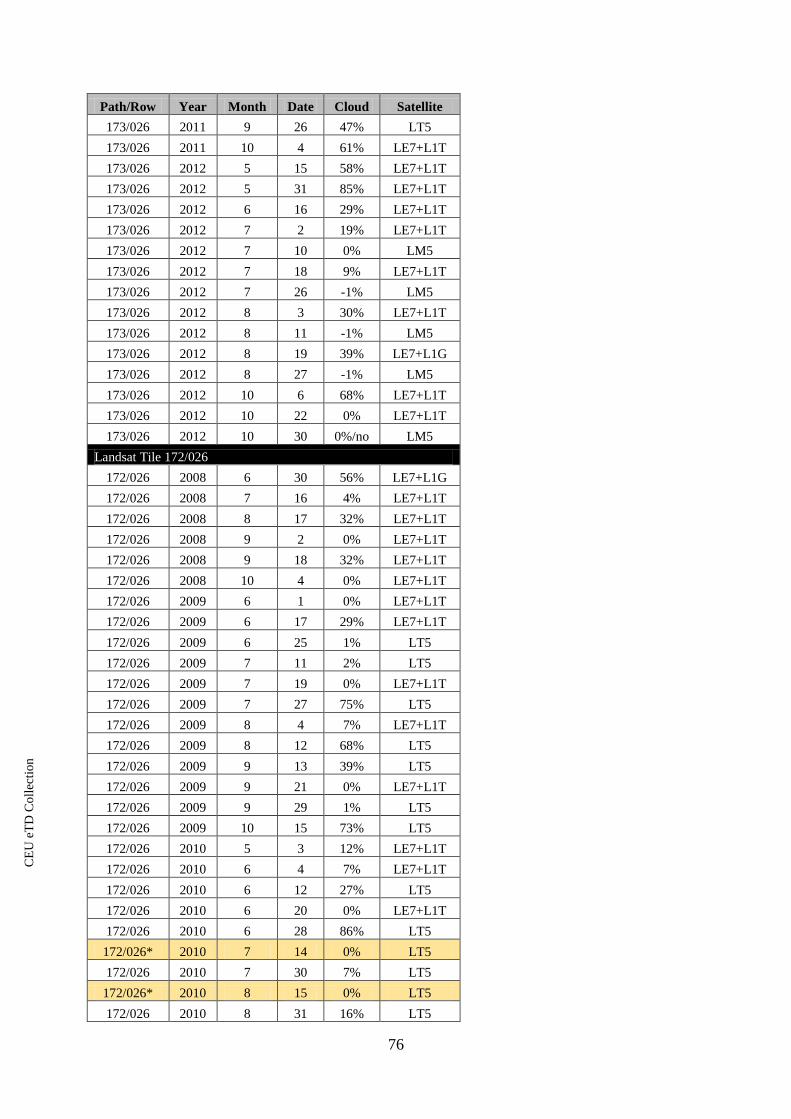
CE

UeT

DC

olle

ctio

n

76

Path/Row Year Month Date Cloud Satellite

173/026 2011 9 26 47% LT5

173/026 2011 10 4 61% LE7+L1T

173/026 2012 5 15 58% LE7+L1T

173/026 2012 5 31 85% LE7+L1T

173/026 2012 6 16 29% LE7+L1T

173/026 2012 7 2 19% LE7+L1T

173/026 2012 7 10 0% LM5

173/026 2012 7 18 9% LE7+L1T

173/026 2012 7 26 -1% LM5

173/026 2012 8 3 30% LE7+L1T

173/026 2012 8 11 -1% LM5

173/026 2012 8 19 39% LE7+L1G

173/026 2012 8 27 -1% LM5

173/026 2012 10 6 68% LE7+L1T

173/026 2012 10 22 0% LE7+L1T

173/026 2012 10 30 0%/no LM5

Landsat Tile 172/026

172/026 2008 6 30 56% LE7+L1G

172/026 2008 7 16 4% LE7+L1T

172/026 2008 8 17 32% LE7+L1T

172/026 2008 9 2 0% LE7+L1T

172/026 2008 9 18 32% LE7+L1T

172/026 2008 10 4 0% LE7+L1T

172/026 2009 6 1 0% LE7+L1T

172/026 2009 6 17 29% LE7+L1T

172/026 2009 6 25 1% LT5

172/026 2009 7 11 2% LT5

172/026 2009 7 19 0% LE7+L1T

172/026 2009 7 27 75% LT5

172/026 2009 8 4 7% LE7+L1T

172/026 2009 8 12 68% LT5

172/026 2009 9 13 39% LT5

172/026 2009 9 21 0% LE7+L1T

172/026 2009 9 29 1% LT5

172/026 2009 10 15 73% LT5

172/026 2010 5 3 12% LE7+L1T

172/026 2010 6 4 7% LE7+L1T

172/026 2010 6 12 27% LT5

172/026 2010 6 20 0% LE7+L1T

172/026 2010 6 28 86% LT5

172/026* 2010 7 14 0% LT5

172/026 2010 7 30 7% LT5

172/026* 2010 8 15 0% LT5

172/026 2010 8 31 16% LT5

CE

UeT

DC

olle

ctio

n

77

Path/Row Year Month Date Cloud Satellite

172/026 2010 9 16 13% LT5

172/026 2010 10 26 3% LE7+L1T

172/026 2011 6 7 30% LE7+L1T

172/026 2011 6 15 27% LT5

172/026 2011 7 1 90% LT5

172/026 2011 7 9 13% LE7+L1T

172/026 2011 7 17 11% LT5

172/026 2011 7 25 28% LE7+L1T

172/026 2011 8 2 0% LT5

172/026 2011 8 10 0% LE7+L1T

172/026 2011 8 18 21% LT5

172/026 2011 8 26 0% LE7+L1T

172/026 2011 9 3 13% LT5

172/026 2011 9 11 32% LE7+L1T

172/026 2011 9 19 13% LT5

172/026 2011 9 27 79% LE7+L1T

172/026 2011 10 29 98% LE7+L1G

172/026 2012 5 8 60% LE7+L1T

172/026 2012 5 24 85% LE7+L1T

172/026 2012 6 9 4% LE7+L1T

172/026 2012 6 25 59% LE7+L1T

172/026 2012 7 11 88% LE7+L1G

172/026 2012 7 27 2% LE7+L1T

172/026 2012 8 4 -1% LM5

172/026 2012 8 12 34% LE7+L1T

172/026 2012 8 20 -1% LM5

172/026 2012 8 28 0% LE7+L1T

172/026 2012 9 5 -1% LM5

172/026 2012 9 13 0% LE7+L1T

172/026 2012 9 21 -1% LM5

172/026 2012 9 29 2% LE7+L1T

172/026 2012 10 15 75% LE7+L1T

172/026 2012 10 23 -1% LM5

172/026 2012 10 31 32% LE7+L1T

Landsat Tile 172/027

172/027 2008 6 14 55% LE7+L1T

172/027 2008 6 30 39% LE7+L1T

172/027 2008 7 16 4% LE7+L1T

172/027 2008 8 17 90% LE7+L1T

172/027 2008 9 2 2% LE7+L1T

172/027 2008 9 18 6% LE7+L1T

172/027 2008 10 4 17% LE7+L1T

172/027 2009 5 16 40% LE7+L1T

172/027 2009 6 1 0% LE7+L1T

CE

UeT

DC

olle

ctio

n

78

Path/Row Year Month Date Cloud Satellite

172/027 2009 6 25 0% LT5

172/027 2009 7 3 1% LE7+L1T

172/027 2009 7 11 8% LT5

172/027 2009 7 19 30% LE7+L1T

172/027 2009 7 27 48% LT5

172/027 2009 8 4 2% LE7+L1T

172/027 2009 8 12 99% LT5

172/027 2009 9 13 7% LT5

172/027 2009 9 21 9% LE7+L1T

172/027 2009 9 29 43% LT5

172/027 2009 10 23 52% LE7-SLC

172/027 2010 5 3 45% LE7+L1T

172/027 2010 6 4 3% LE7+L1T

172/027* 2010 6 12 1% LT5

172/027 2010 6 20 0%no LE7+L1T

172/027 2010 6 28 31% LT5

172/027 2010 7 14 31% LT5

172/027 2010 7 30 0% LT5

172/027 2010 8 7 0% LE7+L1T

172/027* 2010 8 15 7% LT5

172/027 2010 8 23 0% LE7+L1T

172/027 2010 8 31 11% LT5

172/027 2010 9 16 63% LT5

172/027 2010 10 26 1% LE7+L1T

172/027 2011 6 7 31% LE7+L1T

172/027 2011 6 15 35% LT5

172/027 2011 6 23 34% LE7+L1T

172/027 2011 7 1 35% LT5

172/027 2011 7 9 5% LE7+L1T

172/027 2011 7 17 14% LT5

172/027 2011 7 25 80% LE7+L1T

172/027 2011 8 2 1% LT5

172/027 2011 8 10 0% LE7+L1T

172/027 2011 8 18 43% LT5

172/027 2011 8 26 0% LE7+L1T

172/027 2011 9 11 62% LE7-L1G

172/027 2011 9 19 0% LT5

172/027 2011 9 27 18% LE7+L1T

172/027 2011 10 29 100% LE7+L1G

172/027 2012 5 8 79% LE7+L1T

172/027 2012 5 24 99% LE7-L1G

172/027 2012 6 9 16% LE7+L1T

172/027 2012 6 25 16% LE7+L1T

172/027 2012 7 11 92% LE7-L1G

CE

UeT

DC

olle

ctio

n

79

Path/Row Year Month Date Cloud Satellite

172/027 2012 7 27 0% LE7+L1T

172/027 2012 8 4 -1% LM5

172/027 2012 8 12 35% LE7+L1T

172/027 2012 8 20 -1% LM5

172/027 2012 8 28 3% LE7+L1T

172/027 2012 9 5 -1% LM5

172/027 2012 9 13 0% LE7+L1T

172/027 2012 9 21 -1% LM5

172/027 2012 9 29 0% LE7+L1T

172/027 2012 10 15 53% LE7+L1T

172/027 2012 10 23 1% LM5

172/027 2012 10 31 1% LE7+L1T

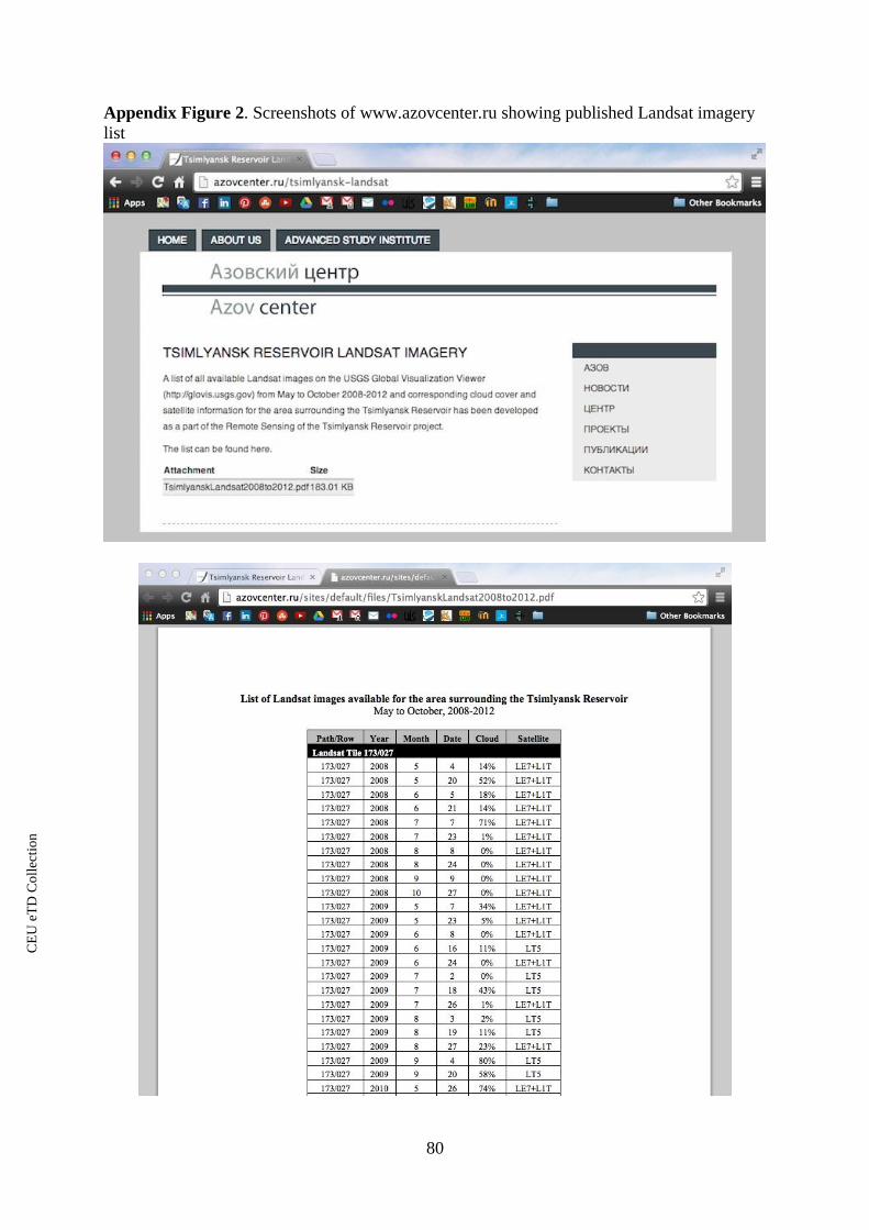
CE

UeT

DC

olle

ctio

n

80

Appendix Figure 2. Screenshots of www.azovcenter.ru showing published Landsat imagery

list

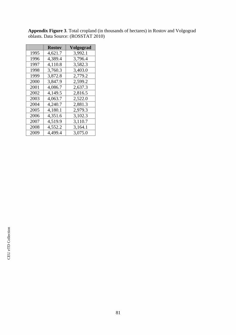
CE

UeT

DC

olle

ctio

n

81

Appendix Figure 3. Total cropland (in thousands of hectares) in Rostov and Volgograd

oblasts. Data Source: (ROSSTAT 2010)

Rostov Volgograd

1995 4,621.7 3,992.1

1996 4,389.4 3,796.4

1997 4,110.8 3,582.3

1998 3,760.3 3,403.0

1999 3,872.8 2,779.2

2000 3,847.9 2,599.2

2001 4,086.7 2,637.3

2002 4,149.5 2,816.5

2003 4,063.7 2,522.0

2004 4,240.7 2,881.3

2005 4,180.1 2,979.3

2006 4,351.6 3,102.3

2007 4,519.9 3,110.7

2008 4,552.2 3,164.1

2009 4,499.4 3,075.0

CE

UeT

DC

olle

ctio

n

82

Appendix Figure 4. Algal bloom events seen in Landsat images. Data Source: (USGS 2014)

#1, 173/026, 14 July 1990, L1 #2, 173/026, 15 August 1990, L1 #3, 172/027, 9 Sept. 1990, L3

#4, 172/027, 25 Sept. 1990, L2

#5, 172/027, 11 October 1990, L3

#6, 173/027, 18 August 1991, L3

#7, 173/027, 19 Sept. 1991, L3

#8, 173/027, 5 October 1991, L1

#9, 173/027, 21 October 1991, L1

#10, 173/027, 6 July 1993, L1

#11, 173/027, 24 Sept. 1993, L2

#12, 173/027, 10 October 1993, L2

CE

UeT

DC

olle

ctio

n

83

#13, 173/026, 26 August 1994, L1

#14, 173/026, 27 Sept. 1994, L2

#15, 172/027, 22 October 1994, L2

#16, 173/027, 29 August 1995, L2

#17, 173/027, 14 July 1996, L2

#18, 173/027, 19 Sept. 1997, L3

#19, 173/026, 20 July 1998, L2

#20, 172/027, 30 August 1998, L2

#21, 172/027, 15 Sept. 1998, L1

#22, 173/026, 3 October 1999, L2

#23, 173/027, 18 August 2000, L2

#24, 172/027, 14 October 2000, L1

CE

UeT

DC

olle

ctio

n

84

#25, 173/027, 6 Sept. 2001, L1

#26, 172/027, 1 October 2001, L1

#27, 173/027, 8 October 2001, L1

#28, 172/027, 28 August 2003, L2

#29, 173/027, 20 Sept. 2003, L3

#30, 172/027, 15 October 2003, L3

#31, 172/027, 5 July 2004, L2

#32, 173/027, 29 August 2004, L1

#33, 172/027, 7 Sept. 2004, L3

#34, 173/027, 14 Sept. 2004, L3

#35, 173/027, 17 Sept. 2005, L1

#36, 173/026, 16 June 2006, L2

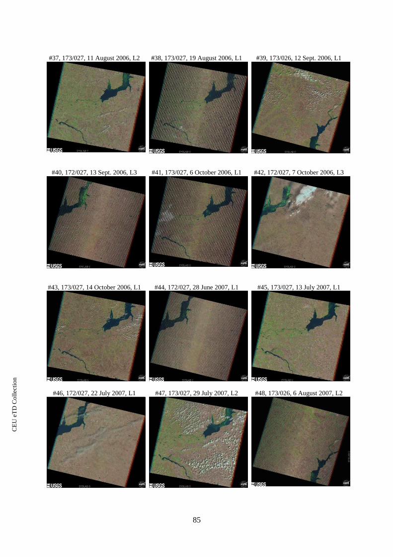
CE

UeT

DC

olle

ctio

n

85

#37, 173/027, 11 August 2006, L2

#38, 173/027, 19 August 2006, L1

#39, 173/026, 12 Sept. 2006, L1

#40, 172/027, 13 Sept. 2006, L3

#41, 173/027, 6 October 2006, L1

#42, 172/027, 7 October 2006, L3

#43, 173/027, 14 October 2006, L1

#44, 172/027, 28 June 2007, L1

#45, 173/027, 13 July 2007, L1

#46, 172/027, 22 July 2007, L1

#47, 173/027, 29 July 2007, L2

#48, 173/026, 6 August 2007, L2

CE

UeT

DC

olle

ctio

n

86

#49, 172/027, 2 Sept. 2008, L3

#50, 173/027, 9 Sept. 2008, L1

#51, 173/027, 24 June 2009, L1

#52, 173/026, 26 July 2009, L1

#53, 173/027, 3 August 2009, L1

#54, 173/027, 19 August 2009, L3

#55, 173/027, 13 Sept. 2009, L1

#56, 172/027, 29 Sept. 2009, L3

#57, 172/027, 30 July 2010, L1

#58, 172/027, 17 July 2011, L1

#59, 173/026, 24 July 2011, L1

#60, 173/027, 17 August 2011, L1

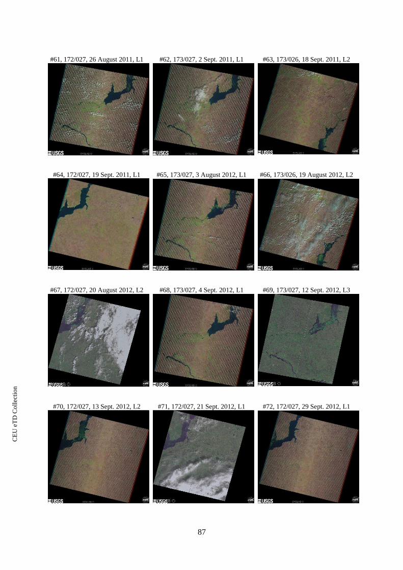
CE

UeT

DC

olle

ctio

n

87

#61, 172/027, 26 August 2011, L1

#62, 173/027, 2 Sept. 2011, L1

#63, 173/026, 18 Sept. 2011, L2

#64, 172/027, 19 Sept. 2011, L1

#65, 173/027, 3 August 2012, L1

#66, 173/026, 19 August 2012, L2

#67, 172/027, 20 August 2012, L2

#68, 173/027, 4 Sept. 2012, L1

#69, 173/027, 12 Sept. 2012, L3

#70, 172/027, 13 Sept. 2012, L2

#71, 172/027, 21 Sept. 2012, L1

#72, 172/027, 29 Sept. 2012, L1

CE

UeT

DC

olle

ctio

n

88

#73, 173/027, 22 October 2012, L2 #74, 173/027, 27 June 2013, L3 #75, 172/027, 6 July 2013, L1

#76, 173/026, 13 July 2013, L1

#77, 173/027, 6 August 2013, L1

#78, 172/027, 7 August 2013, L1

#79, 173/027, 14 August 2013, L1

#80, 172/027, 23 August 2013, L1

#81, 173/027, 1 October 2013, L3

#82, 172/027, 10 October 2013, L2

CE

UeT

DC

olle

ctio

n

89

Appendix Figure 5. Screenshots of www.azovcenter.ru showing published algal bloom

images identified through satellite imagery.

CE

UeT

DC

olle

ctio

n

90

Appendix Figure 6. Determination of algal bloom extent.

# Tile Date Month Satellite Bloom Level Amount of Reservoir Level

1 173_026 14-Jul-90 July LT5 Minor Small section 1

2 173_026 15-Aug-90 August LT5 Minor Small section 1

3 172_027 9-Sep-90 September LT5 Extensive Large section 3

4 172_027 25-Sep-90 September LT5 Moderate Large section 2

5 172_027 11-Oct-90 October LT5 Extensive Large section 3

6 173_027 18-Aug-91 August LT5 Extensive Large section 3

7 173_027 19-Sep-91 September LT5 Extensive Large section 3

8 173_027 5-Oct-91 October LT5 Minor Small section 1

9 173_027 21-Oct-91 October LT5 Minor Medium section 1

10 173_026 6-Jul-93 July LT5 Minor Small section 1

11 173_027 24-Sep-93 September LT5 Moderate Large section 2

12 173_027 10-Oct-93 October LT5 Moderate Medium section 2

13 173_026 26-Aug-94 August LT5 Minor Small section 1

14 173_026 27-Sep-94 September LT5 Moderate Medium section 2

15 172_027 22-Oct-94 October LT5 Moderate Medium section 2

16 173_027 29-Aug-95 August LT5 Moderate Large section 2

17 173_027 14-Jul-96 July LT5 Moderate Medium section 2

18 173_027 19-Sep-97 September LT5 Extensive Large section 3

19 173_026 20-Jul-98 July LT5 Moderate Large section 2

20 172_027 30-Aug-98 August LT5 Moderate Medium section 2

21 172_027 15-Sep-98 September LT5 Minor Small section 1

22 173_026 3-Oct-99 October LE7 Moderate Medium section 2

23 173_027 18-Aug-00 August LE7 Moderate Large section 2

24 172_027 14-Oct-00 October LE7 Minor Small section 1

25 173_027 6-Sep-01 September LE7 Minor Medium section 1

26 172_027 1-Oct-01 October LE7 Minor Small section 1

27 173_027 8-Oct-01 October LE7 Minor Small section 1

28 172_027 28-Aug-03 August LT5 Moderate Large section 2

29 173_027 20-Sep-03 September LT5 Extensive Large section 3

30 172_027 15-Oct-03 October LT5 Extensive Large section 3

31 172_027 5-Jul-04 July LE7 Moderate Medium section 2

32 173_027 29-Aug-04 August LE7 Minor Medium section 1

33 172_027 7-Sep-04 September LE7 Extensive Large section 3

34 173_027 14-Sep-04 September LE7 Extensive Large section 3

35 173_027 17-Sep-05 September LE7 Minor Medium section 1

36 173_026 16-Jun-06 June LE7 Moderate Medium section 2

37 173_027 11-Aug-06 August LT5 Moderate Medium section 2

38 173_027 19-Aug-06 August LE7 Minor Small section 1

39 173_026 12-Sep-06 September LT5 Minor Small section 1

40 172_027 13-Sep-06 September LE7 Extensive Large section 3

41 173_027 6-Oct-06 October LE7 Minor Small section 1

42 172_027 7-Oct-06 October LT5 Extensive Large section 3

43 173_027 14-Oct-06 October LT5 Minor Small section 1

44 172_027 28-Jun-07 June LE7 Minor Medium section 1

45 173_027 13-Jul-07 July LT5 Minor Small section 1

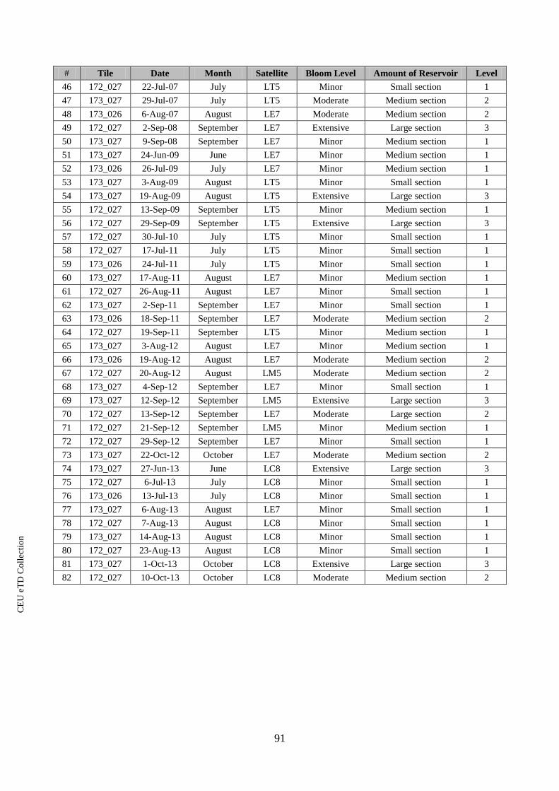
CE

UeT

DC

olle

ctio

n

91

# Tile Date Month Satellite Bloom Level Amount of Reservoir Level

46 172_027 22-Jul-07 July LT5 Minor Small section 1

47 173_027 29-Jul-07 July LT5 Moderate Medium section 2

48 173_026 6-Aug-07 August LE7 Moderate Medium section 2

49 172_027 2-Sep-08 September LE7 Extensive Large section 3

50 173_027 9-Sep-08 September LE7 Minor Medium section 1

51 173_027 24-Jun-09 June LE7 Minor Medium section 1

52 173_026 26-Jul-09 July LE7 Minor Medium section 1

53 173_027 3-Aug-09 August LT5 Minor Small section 1

54 173_027 19-Aug-09 August LT5 Extensive Large section 3

55 172_027 13-Sep-09 September LT5 Minor Medium section 1

56 172_027 29-Sep-09 September LT5 Extensive Large section 3

57 172_027 30-Jul-10 July LT5 Minor Small section 1

58 172_027 17-Jul-11 July LT5 Minor Small section 1

59 173_026 24-Jul-11 July LT5 Minor Small section 1

60 173_027 17-Aug-11 August LE7 Minor Medium section 1

61 172_027 26-Aug-11 August LE7 Minor Small section 1

62 173_027 2-Sep-11 September LE7 Minor Small section 1

63 173_026 18-Sep-11 September LE7 Moderate Medium section 2

64 172_027 19-Sep-11 September LT5 Minor Medium section 1

65 173_027 3-Aug-12 August LE7 Minor Medium section 1

66 173_026 19-Aug-12 August LE7 Moderate Medium section 2

67 172_027 20-Aug-12 August LM5 Moderate Medium section 2

68 173_027 4-Sep-12 September LE7 Minor Small section 1

69 173_027 12-Sep-12 September LM5 Extensive Large section 3

70 172_027 13-Sep-12 September LE7 Moderate Large section 2

71 172_027 21-Sep-12 September LM5 Minor Medium section 1

72 172_027 29-Sep-12 September LE7 Minor Small section 1

73 173_027 22-Oct-12 October LE7 Moderate Medium section 2

74 173_027 27-Jun-13 June LC8 Extensive Large section 3

75 172_027 6-Jul-13 July LC8 Minor Small section 1

76 173_026 13-Jul-13 July LC8 Minor Small section 1

77 173_027 6-Aug-13 August LE7 Minor Small section 1

78 172_027 7-Aug-13 August LC8 Minor Small section 1

79 173_027 14-Aug-13 August LC8 Minor Small section 1

80 172_027 23-Aug-13 August LC8 Minor Small section 1

81 173_027 1-Oct-13 October LC8 Extensive Large section 3

82 172_027 10-Oct-13 October LC8 Moderate Medium section 2

CE

UeT

DC

olle

ctio

n

92

Appendix Figure 7. Precipitation vs. algal bloom graphs, 1998-2013. Data Source: (USGS

2014; NASA 2013a)

CE

UeT

DC

olle

ctio

n

93

Note: there were

no algal blooms

identified in 2002.

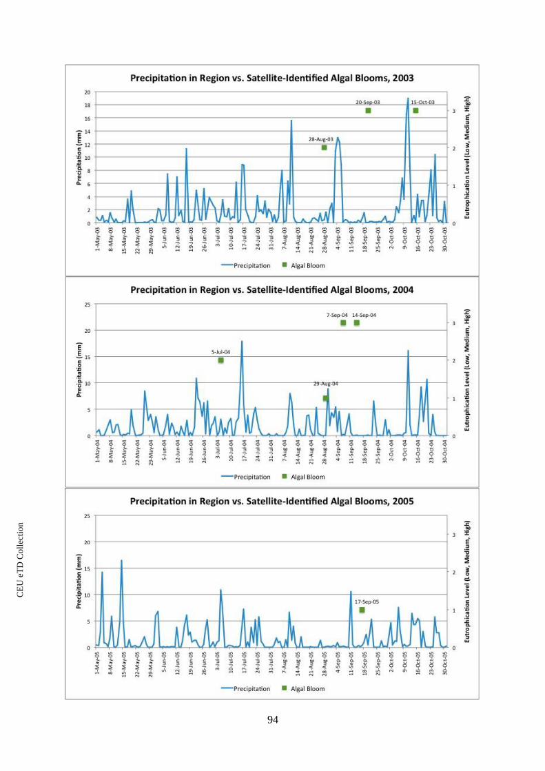
CE

UeT

DC

olle

ctio

n

94

CE

UeT

DC

olle

ctio

n

95

CE

UeT

DC

olle

ctio

n

96

CE

UeT

DC

olle

ctio

n

97