a tool for optimized layout of °at cable harnesses for...
TRANSCRIPT

Master’s thesis
A tool for optimized layout of flat cableharnesses for future on-board cabling
systems in cars.
by Tobias Marciszko
LITH-IDA-EX–04/027–SE
2004-04-16

Master’s thesis
A tool for optimized layout of flat cableharnesses for future on-board cabling
systems in cars.
by Tobias Marciszko
LiTH-IDA-EX–04/027–SE
Supervisor: Tobias RaithelResearch and Technology, REM/EHat DaimlerChrysler AG
Examiner: Assoc. Prof. Dr. Christoph KesslerDepartment of Computer and InformationScienceat Linkopings universitet

Avdelning, InstitutionDivision, Department
DatumDate
Sprak
Language
2 Svenska/Swedish
2 Engelska/English
2
RapporttypReport category
2 Licentiatavhandling
2 Examensarbete
2 C-uppsats
2 D-uppsats
2 Ovrig rapport
2
URL for elektronisk version
ISBN
ISRN
Serietitel och serienummerTitle of series, numbering
ISSN
Titel
Title
ForfattareAuthor
SammanfattningAbstract
NyckelordKeywords
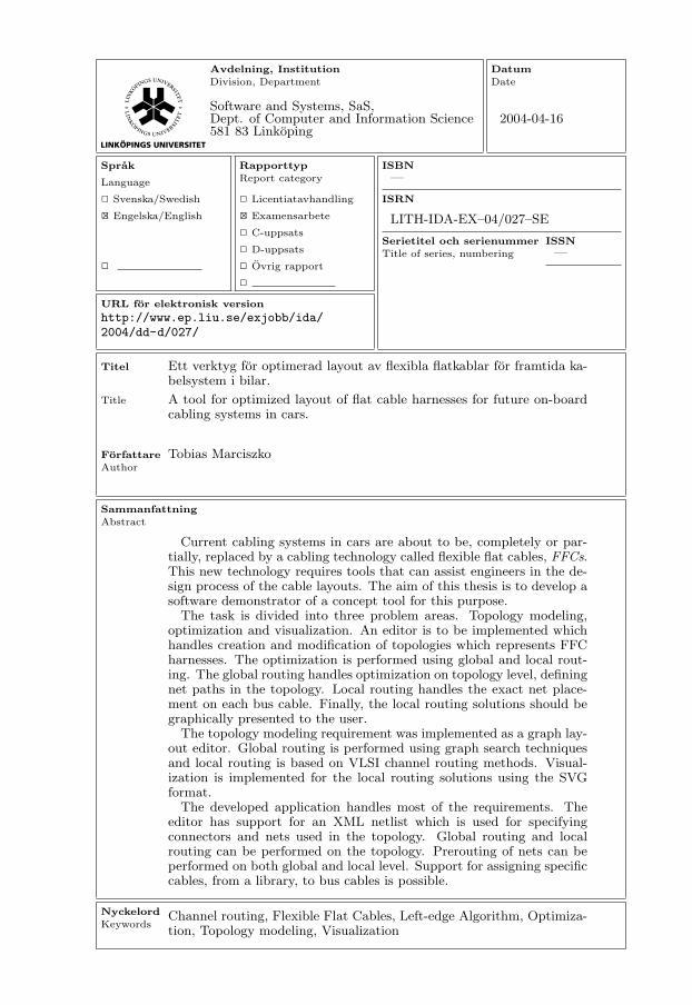
Current cabling systems in cars are about to be, completely or par-tially, replaced by a cabling technology called flexible flat cables, FFCs.This new technology requires tools that can assist engineers in the de-sign process of the cable layouts. The aim of this thesis is to develop asoftware demonstrator of a concept tool for this purpose.
The task is divided into three problem areas. Topology modeling,optimization and visualization. An editor is to be implemented whichhandles creation and modification of topologies which represents FFCharnesses. The optimization is performed using global and local rout-ing. The global routing handles optimization on topology level, definingnet paths in the topology. Local routing handles the exact net place-ment on each bus cable. Finally, the local routing solutions should begraphically presented to the user.
The topology modeling requirement was implemented as a graph lay-out editor. Global routing is performed using graph search techniquesand local routing is based on VLSI channel routing methods. Visual-ization is implemented for the local routing solutions using the SVGformat.
The developed application handles most of the requirements. Theeditor has support for an XML netlist which is used for specifyingconnectors and nets used in the topology. Global routing and localrouting can be performed on the topology. Prerouting of nets can beperformed on both global and local level. Support for assigning specificcables, from a library, to bus cables is possible.
Software and Systems, SaS,Dept. of Computer and Information Science581 83 Linkoping
2004-04-16
—
LITH-IDA-EX–04/027–SE
—
http://www.ep.liu.se/exjobb/ida/2004/dd-d/027/
2004-04-16
A tool for optimized layout of flat cable harnesses for future on-boardcabling systems in cars.
Ett verktyg for optimerad layout av flexibla flatkablar for framtida ka-belsystem i bilar.
Tobias Marciszko
××
Channel routing, Flexible Flat Cables, Left-edge Algorithm, Optimiza-tion, Topology modeling, Visualization


Abstract
Current cabling systems in cars are about to be, completely or partially,replaced by a cabling technology called flexible flat cables, FFCs. Thisnew technology requires tools that can assist engineers in the designprocess of the cable layouts. The aim of this thesis is to develop asoftware demonstrator of a concept tool for this purpose.
The task is divided into three problem areas. Topology modeling,optimization and visualization. An editor is to be implemented whichhandles creation and modification of topologies which represents FFCharnesses. The optimization is performed using global and local rout-ing. The global routing handles optimization on topology level, definingnet paths in the topology. Local routing handles the exact net place-ment on each bus cable. Finally, the local routing solutions should begraphically presented to the user.
The topology modeling requirement was implemented as a graphlayout editor. Global routing is performed using graph search tech-niques and local routing is based on VLSI channel routing methods.Visualization is implemented for the local routing solutions using theSVG format.
The developed application handles most of the requirements. Theeditor has support for an XML netlist which is used for specifyingconnectors and nets used in the topology. Global routing and localrouting can be performed on the topology. Prerouting of nets can beperformed on both global and local level. Support for assigning specificcables, from a library, to bus cables is possible.
Keywords: Channel routing, Flexible Flat Cables, Left-edge Algo-rithm, Optimization, Topology modeling, Visualization
v

vi
Acknowledgements
I would like to thank everyone that has contributed to this thesis; Pro-fessor Evangeline Young Fung Yu at The Chinese University of HongKong and assistant professor Hai Zhou at Northwestern University inEvanston, USA, for letting me use parts of their lecture material. Iwould like to thank everyone that I got to know, Swedes and Germans,during my stay in Esslingen. Especially the people in Team Thelen andall you guys from the REM/EP department. You know who you are!I would also like to thank my supervisor, Tobias Raithel, for all thesupport and help throughout my stay. Finally, I would like to thankmy examiner, Christoph Kessler and my two opponents, Johan Wigertand Benoit Daviaud for the comments and help in finalizing the report.
This thesis could not have been realized without the support frommy friends, my girlfriend and my family.
Linkoping, April 2004Tobias Marciszko
vii

viii
Contents
Abstract v
Acknowledgements vii
1 Introduction 11.1 Background and aim . . . . . . . . . . . . . . . . . . . . 1
1.1.1 Flexible flat cables . . . . . . . . . . . . . . . . . 11.2 Problem definition . . . . . . . . . . . . . . . . . . . . . 41.3 Previous work . . . . . . . . . . . . . . . . . . . . . . . . 41.4 Thesis outline . . . . . . . . . . . . . . . . . . . . . . . . 5
2 Theory 72.1 Channel routing . . . . . . . . . . . . . . . . . . . . . . 7
2.1.1 Introduction and terminology . . . . . . . . . . . 72.1.2 Constraint graphs . . . . . . . . . . . . . . . . . 82.1.3 Left-edge algorithm . . . . . . . . . . . . . . . . 102.1.4 Constrained left-edge algorithm . . . . . . . . . . 102.1.5 Dogleg algorithm . . . . . . . . . . . . . . . . . . 112.1.6 Other algorithms . . . . . . . . . . . . . . . . . . 12
2.2 Graph searching . . . . . . . . . . . . . . . . . . . . . . 152.2.1 Definition . . . . . . . . . . . . . . . . . . . . . . 152.2.2 Depth-first search . . . . . . . . . . . . . . . . . 152.2.3 Breadth-first search . . . . . . . . . . . . . . . . 162.2.4 Least-cost path . . . . . . . . . . . . . . . . . . . 16
3 Requirements 193.1 Introduction . . . . . . . . . . . . . . . . . . . . . . . . . 193.2 Domain model . . . . . . . . . . . . . . . . . . . . . . . 193.3 Topology modeling . . . . . . . . . . . . . . . . . . . . . 20
3.3.1 Topology modeling use cases . . . . . . . . . . . 213.4 Optimization . . . . . . . . . . . . . . . . . . . . . . . . 22
3.4.1 Global routing . . . . . . . . . . . . . . . . . . . 223.4.2 Local routing . . . . . . . . . . . . . . . . . . . . 23
ix

x CONTENTS
3.5 Visualization . . . . . . . . . . . . . . . . . . . . . . . . 24
4 Implementation 274.1 Previous work . . . . . . . . . . . . . . . . . . . . . . . . 274.2 Topology modeling . . . . . . . . . . . . . . . . . . . . . 27
4.2.1 Introduction . . . . . . . . . . . . . . . . . . . . 284.2.2 Functionality . . . . . . . . . . . . . . . . . . . . 294.2.3 Framework limitations . . . . . . . . . . . . . . . 304.2.4 Attributes . . . . . . . . . . . . . . . . . . . . . . 30
4.3 Global routing . . . . . . . . . . . . . . . . . . . . . . . 314.3.1 Introduction . . . . . . . . . . . . . . . . . . . . 324.3.2 Cost functions . . . . . . . . . . . . . . . . . . . 324.3.3 Global routing algorithm . . . . . . . . . . . . . 344.3.4 Virtual connectors . . . . . . . . . . . . . . . . . 354.3.5 Global prerouting . . . . . . . . . . . . . . . . . 35
4.4 Local routing . . . . . . . . . . . . . . . . . . . . . . . . 374.4.1 Channel routing . . . . . . . . . . . . . . . . . . 374.4.2 Topology parsing and validation . . . . . . . . . 384.4.3 Local prerouting . . . . . . . . . . . . . . . . . . 404.4.4 Cable type selection . . . . . . . . . . . . . . . . 41
4.5 Via placement . . . . . . . . . . . . . . . . . . . . . . . . 424.6 Visualization . . . . . . . . . . . . . . . . . . . . . . . . 454.7 Application examples . . . . . . . . . . . . . . . . . . . . 474.8 Class overview . . . . . . . . . . . . . . . . . . . . . . . 47
5 Summary 535.1 Future work . . . . . . . . . . . . . . . . . . . . . . . . . 54
Bibliography 55
A Glossary 59
B Netlist example 63
C Cable library example 65
List of Figures
1.1 Comparison of a round cable and a FFC harness. . . . . 21.2 FFC connection matrices. . . . . . . . . . . . . . . . . . 31.3 Different types of FFCs with and without connectors. . 41.4 A complete FFC car cockpit harness. . . . . . . . . . . . 5
2.1 Channel routing terminology. Modified from Young FungYu [20]. . . . . . . . . . . . . . . . . . . . . . . . . . . . 8
2.2 A channel and its corresponding horizontal constraintgraph (HCG). Zhou [22]. . . . . . . . . . . . . . . . . . . 9
2.3 A channel and its corresponding vertical constraint graph(VCG). Zhou [22]. . . . . . . . . . . . . . . . . . . . . . 10
2.4 Example of the left-edge algorihtm. Young Fung Yu [20]. 112.5 Suboptimal solution from the constrained left-edge algo-
rithm. Kernighan et al. [10]. . . . . . . . . . . . . . . . . 132.6 A channel with a cyclic constraint and its corresponding
VCG. Young Fung Yu [20]. . . . . . . . . . . . . . . . . 132.7 Reducing channel width using doglegs. Matuszewski [13]. 14
3.1 FFC harness and channel routing domains. . . . . . . . 203.2 Example of a FFC-topology with connection matrices,
buses and connectors. Modified from Raithel [17]. . . . . 213.3 Use cases for topology modeling. . . . . . . . . . . . . . 223.4 Use cases for modification of the topology. . . . . . . . . 233.5 Global routing finding a net path in the topology. . . . . 243.6 Visualization example. Raithel [16]. . . . . . . . . . . . 25
4.1 Representation of real world elements in the topology. . 284.2 Screenshot of the implemented editor with a modeled
FFC harness. . . . . . . . . . . . . . . . . . . . . . . . . 294.3 Model-View-Controller (MVC). Alder [2]. . . . . . . . . 314.4 Topology graph with edge costs. . . . . . . . . . . . . . 334.5 Topology graph in the original representation. . . . . . . 334.6 Graph after conversion, showing edge costs. . . . . . . . 34
xi

xii LIST OF FIGURES
4.7 Prerouting input for each net. . . . . . . . . . . . . . . . 364.8 The channel routing representation of a bus cable and a
solution with the left-edge algorithm. . . . . . . . . . . . 384.9 Invalid buses, not detected by the topology validation. . 404.10 Possibility to assign an FFC cable to a bus. Here with
the cable library from Appendix C. . . . . . . . . . . . . 414.11 Connection matrices with incorrect via placement. . . . 434.12 Connection matrices with correct via placement. . . . . 444.13 A routing solution using the SVG format. . . . . . . . . 454.14 The generated HTML document for easy access to solu-
tions and reports. . . . . . . . . . . . . . . . . . . . . . . 464.15 Modeled topology of the cockpit in Figure 1.4. . . . . . 484.16 Excerpt from the local routing solution of the cockpit in
Figure 1.4. . . . . . . . . . . . . . . . . . . . . . . . . . . 494.17 Overview of the local routing solution of the cockpit in
Figure 1.4. . . . . . . . . . . . . . . . . . . . . . . . . . . 504.18 Overview of the main classes in the application. . . . . . 51

Chapter 1
Introduction
This thesis has been carried out at the DaimlerChrysler departmentREM/EH, Electronics Hardware, in Esslingen am Neckar, Germany.LATEX has been used to create this document.
1.1 Background and aim
Current cabling systems in cars are about to be, completely or partially,replaced by newer technology. Flexible flat cables, FFCs, is one ofthe new technologies which is getting ready for being introduced intoserial production. This new technology requires tools that can assistengineers in the design process of the cable layouts. Therefore, the aimof this thesis is to develop a software demonstrator of a concept toolfor modeling and optimization of flexible flat cable layouts.
1.1.1 Flexible flat cables
A flexible flat cable, FFC, is a cable made out of PVC or polyurethanematerial with copper wires laid out horizontally. An FFC harness is aset of FFCs connected together allowing signals to reach connectors oneach cable. According to Adams et al. [1], the development of flexibleflat cables has reached a point where they are applicable in vehicles.The advantages of the new cabling system are reduction of volumeand weight. Furthermore, cost can be reduced through automation ofproduction of the harness and of the mounting at the car assemblyline. In this thesis, the terms FFC, flexible flat cable and flat cable areused interchangeably. To start this introduction we present the FFCcompared to the common cabling system, the round wires. In Figure 1.1we can see the differences, and similarities, between the round wire andits corresponding FFC harness.
1

2 Chapter 1. Introduction
Figure 1.1: Comparison of a round cable and a FFC harness.
The most significant difference between the FFC and the roundwires is that the FFC wires are not bundled together. Instead, all wiresare laid out horizontally with an isolation material in between and onthe top and bottom. This means that the FFC can have any numberof wires, although the current maximum is 32 wires with a spacing of2,54 mm, Adams et al. [1]. The wires, which is made out of copper, canhave different width and thereby different cross section area in whichthe resistance of the wires can be influenced. The maximum width ofa wire is 19 mm which gives a cross section area of 4 mm2. This meansthat the ampacity rating of the wire is 50 A, see Adams et al. [1], i.e.50 A can be transmitted without overloading the wire.
The design of the FFC makes it possible to connect cables to eachother. A set of connected cables is called a harness. The connectionareas are called connection matrices which can be seen in Figure 1.2.In this figure, two cables are connected to a third cable which meansthere are two connection matrices. In each of the matrices there arewelding points which connect the desired wires together.

1.1. Background and aim 3
Figure 1.2: FFC connection matrices.
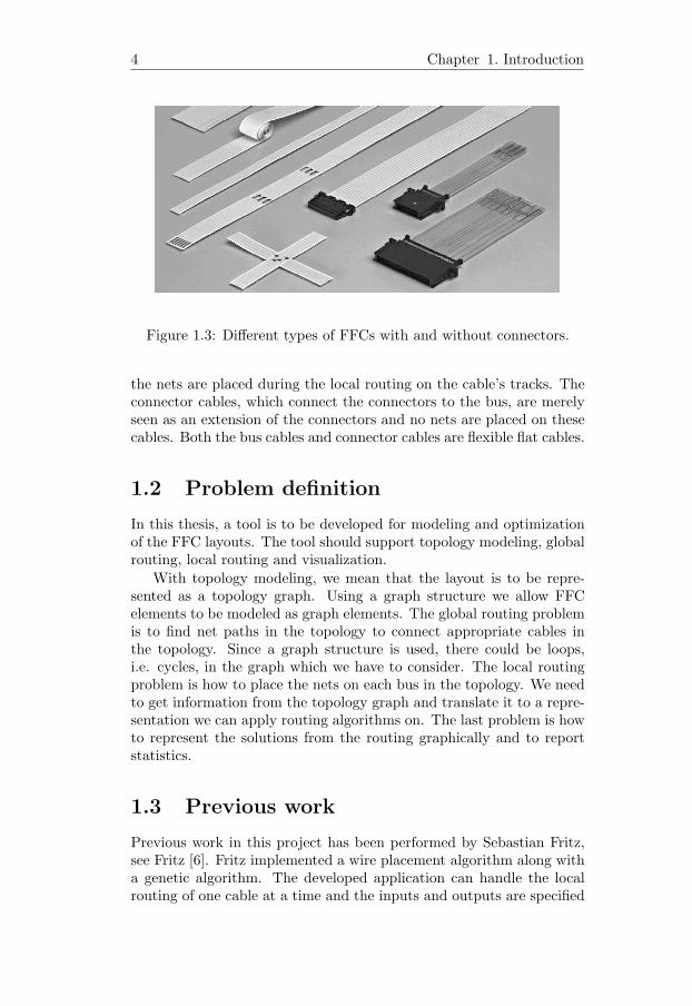
Tracks are the rows in the cable which carry the wires. One trackcan consist of one wire, or several wires with the use of punched-outholes. By connecting several cables to each other, we can form netsof wires making it possible to have multiple connectors using the samesignal. Net is the term for the connected tracks, on one or more cables,that carry the same signal. The connectors in the FFC harness allowto externally access the tracks of a cable at a cable endpoint. Theyconsist of a number of pins. Each pin has a defined width which definesthe minimum track width required to carry the signal. The pins alsohave a net number. This net number defines which of the pins, fromseveral connectors in the harness, that should be connected to formnets. Typical FFC connectors along with a variety of different FFCcables can be seen in Figure 1.3. In this figure we also notice the use ofpunched-out holes in one of the cables. This method of splitting wiresmakes the cable usage more efficient since one track can carry morethan one net.
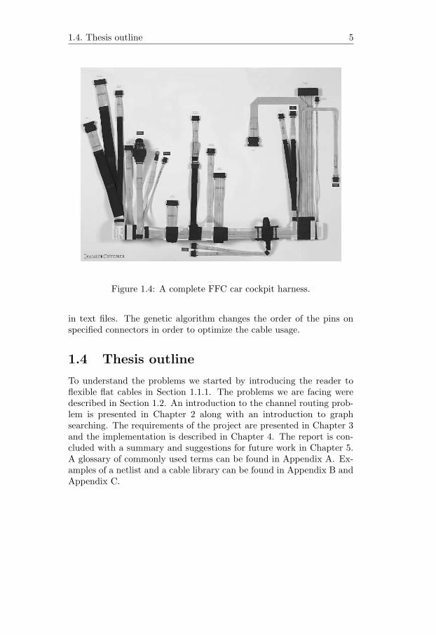
To end the introduction of flexible flat cables, we present an exam-ple of how a complete FFC harness could look like. In Figure 1.4 wesee a harness for a car cockpit, complete with connectors and isolationmaterial on the connection matrices to cover the welding points. To-gether with this picture, we introduce the terms bus cable, or bus, andconnector cables. The bus cable in this picture is the bottom-most ca-ble. As we will see, in Section 2.1 and Chapter 3, it is in the bus cable
4 Chapter 1. Introduction
Figure 1.3: Different types of FFCs with and without connectors.
the nets are placed during the local routing on the cable’s tracks. Theconnector cables, which connect the connectors to the bus, are merelyseen as an extension of the connectors and no nets are placed on thesecables. Both the bus cables and connector cables are flexible flat cables.
1.2 Problem definition
In this thesis, a tool is to be developed for modeling and optimizationof the FFC layouts. The tool should support topology modeling, globalrouting, local routing and visualization.
With topology modeling, we mean that the layout is to be repre-sented as a topology graph. Using a graph structure we allow FFCelements to be modeled as graph elements. The global routing problemis to find net paths in the topology to connect appropriate cables inthe topology. Since a graph structure is used, there could be loops,i.e. cycles, in the graph which we have to consider. The local routingproblem is how to place the nets on each bus in the topology. We needto get information from the topology graph and translate it to a repre-sentation we can apply routing algorithms on. The last problem is howto represent the solutions from the routing graphically and to reportstatistics.
1.3 Previous work
Previous work in this project has been performed by Sebastian Fritz,see Fritz [6]. Fritz implemented a wire placement algorithm along witha genetic algorithm. The developed application can handle the localrouting of one cable at a time and the inputs and outputs are specified
1.4. Thesis outline 5
Figure 1.4: A complete FFC car cockpit harness.
in text files. The genetic algorithm changes the order of the pins onspecified connectors in order to optimize the cable usage.
1.4 Thesis outline
To understand the problems we started by introducing the reader toflexible flat cables in Section 1.1.1. The problems we are facing weredescribed in Section 1.2. An introduction to the channel routing prob-lem is presented in Chapter 2 along with an introduction to graphsearching. The requirements of the project are presented in Chapter 3and the implementation is described in Chapter 4. The report is con-cluded with a summary and suggestions for future work in Chapter 5.A glossary of commonly used terms can be found in Appendix A. Ex-amples of a netlist and a cable library can be found in Appendix B andAppendix C.

6 Chapter 1. Introduction

Chapter 2
Theory
This chapter introduces the reader to the VLSI channel routing problemin which we can find relevant foundations and formalizations for theproblems in this project. Also, a brief introduction to graph searchingis presented.
2.1 Channel routing
This section describes the fundamentals of channel routing. An intro-duction is given along with routing terminology. We then discuss theconstraint graphs that characterize the channel routing problem. Thesection is concluded by describing commonly used algorithms alongwith other alternative algorithms.
2.1.1 Introduction and terminology
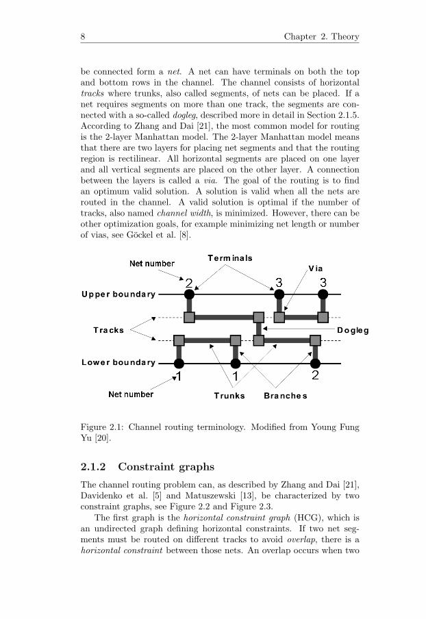
The channel routing problem (CRP) is a special type of detailed routingmainly used in VLSI design, see Zhang and Dai [21] and Gockel et al. [8].In channel routing, two rows of terminals exist on the top and on thebottom of a channel, see Figure 2.1. Each terminal holds a number,the net number. All the terminals with the same net number should beconnected inside the channel. The area inside the channel is called therouting region, or routing area.
The channel routing problem can be described by specifying twolists of n net numbers, one for the top of the channel and one for thebottom of the channel, Smith [18]. The net numbers’ positions in thelist also gives the horizontal position in the channel. If there is a ter-minal with net number 0, the terminal is vacant, i.e. the terminal shallnot be connected, see also Figure 2.2. The main task of the routingis to connect terminals inside the channel. All terminals that should
7
8 Chapter 2. Theory
be connected form a net. A net can have terminals on both the topand bottom rows in the channel. The channel consists of horizontaltracks where trunks, also called segments, of nets can be placed. If anet requires segments on more than one track, the segments are con-nected with a so-called dogleg, described more in detail in Section 2.1.5.According to Zhang and Dai [21], the most common model for routingis the 2-layer Manhattan model. The 2-layer Manhattan model meansthat there are two layers for placing net segments and that the routingregion is rectilinear. All horizontal segments are placed on one layerand all vertical segments are placed on the other layer. A connectionbetween the layers is called a via. The goal of the routing is to findan optimum valid solution. A solution is valid when all the nets arerouted in the channel. A valid solution is optimal if the number oftracks, also named channel width, is minimized. However, there can beother optimization goals, for example minimizing net length or numberof vias, see Gockel et al. [8].
Figure 2.1: Channel routing terminology. Modified from Young FungYu [20].
2.1.2 Constraint graphs
The channel routing problem can, as described by Zhang and Dai [21],Davidenko et al. [5] and Matuszewski [13], be characterized by twoconstraint graphs, see Figure 2.2 and Figure 2.3.
The first graph is the horizontal constraint graph (HCG), which isan undirected graph defining horizontal constraints. If two net seg-ments must be routed on different tracks to avoid overlap, there is ahorizontal constraint between those nets. An overlap occurs when two
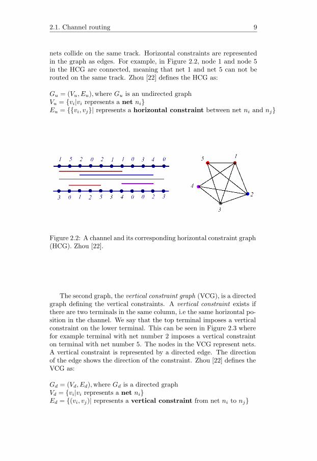
2.1. Channel routing 9
nets collide on the same track. Horizontal constraints are representedin the graph as edges. For example, in Figure 2.2, node 1 and node 5in the HCG are connected, meaning that net 1 and net 5 can not berouted on the same track. Zhou [22] defines the HCG as:
Gu = (Vu, Eu), where Gu is an undirected graphVu = {vi|vi represents a net ni}Eu = {{vi, vj}| represents a horizontal constraint between net ni and nj}
Figure 2.2: A channel and its corresponding horizontal constraint graph(HCG). Zhou [22].
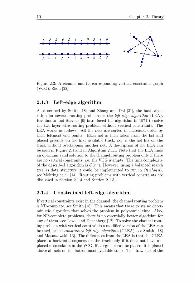
The second graph, the vertical constraint graph (VCG), is a directedgraph defining the vertical constraints. A vertical constraint exists ifthere are two terminals in the same column, i.e the same horizontal po-sition in the channel. We say that the top terminal imposes a verticalconstraint on the lower terminal. This can be seen in Figure 2.3 wherefor example terminal with net number 2 imposes a vertical constrainton terminal with net number 5. The nodes in the VCG represent nets.A vertical constraint is represented by a directed edge. The directionof the edge shows the direction of the constraint. Zhou [22] defines theVCG as:
Gd = (Vd, Ed), where Gd is a directed graphVd = {vi|vi represents a net ni}Ed = {(vi, vj)| represents a vertical constraint from net ni to nj}
10 Chapter 2. Theory
Figure 2.3: A channel and its corresponding vertical constraint graph(VCG). Zhou [22].
2.1.3 Left-edge algorithm
As described by Smith [18] and Zhang and Dai [21], the basis algo-rithm for several routing problems is the left-edge algorithm (LEA).Hashimoto and Stevens [9] introduced the algorithm in 1971 to solvethe two layer wire routing problem without vertical constraints. TheLEA works as follows. All the nets are sorted in increased order bytheir leftmost end points. Each net is then taken from the list andplaced greedily on the first available track, i.e. if the net fits on thetrack without overlapping another net. A description of the LEA canbe seen in Figure 2.4 and in Algorithm 2.1.1. Note that the LEA findsan optimum valid solution to the channel routing problem only if thereare no vertical constraints, i.e. the VCG is empty. The time complexityof the described algorithm is O(n2). However, using a balanced searchtree as data structure it could be implemented to run in O(n log n),see Mohring et al. [14]. Routing problems with vertical constraints arediscussed in Section 2.1.4 and Section 2.1.5.
2.1.4 Constrained left-edge algorithm
If vertical constraints exist in the channel, the channel routing problemis NP-complete, see Smith [18]. This means that there exists no deter-ministic algorithm that solves the problem in polynomial time. Also,for NP-complete problems, there is no essentially better algorithm forany of them, see Lewis and Denenberg [12]. To solve the channel rout-ing problem with vertical constraints a modified version of the LEA canbe used, called constrained left-edge algorithm (CLEA), see Smith [18]and Matuszewski [13]. The differences from the LEA is that the CLEAplaces a horizontal segment on the track only if it does not have un-placed descendants in the VCG. If a segment can be placed, it is placedabove all nets on the bottommost available track. The drawback of the

2.1. Channel routing 11
Figure 2.4: Example of the left-edge algorihtm. Young Fung Yu [20].
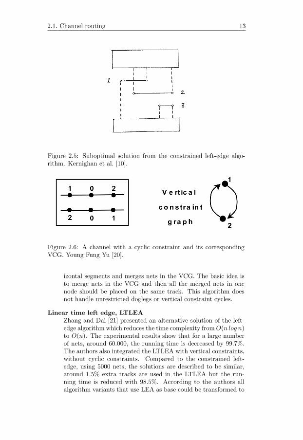
CLEA is that it does not handle cyclic constraints (vertical constraintcycles) which means that there is a cycle in the VCG, see Figure 2.6.One solution to the problem is the dogleg algorithm by Deutsch [4]which is discussed in Section 2.1.5. Although, when taking the verticalconstraints into account, it is not guaranteed that the algorithm findsan optimum solution (minimum number of tracks), see Kernighan etal. [10]. For example, in Figure 2.5, the solution is not an optimumsolution since it is trivial to see that there is an optimum solution withonly two tracks.
2.1.5 Dogleg algorithm
The dogleg algorithm by Deutsch [4], see also Persky et al. [15], is analgorithm based on the constrained left-edge algorithm to solve therouting problem with vertical constraints, including cyclic constraints.The dogleg algorithm allows net segments to be placed on not onlyone track. This means that each net is divided into 2-terminal sub-nets which can be placed on different tracks. The dogleg algorithmuses a range parameter to control the behavior of the algorithm, seeDeutsch [4]. This parameter represents the minimum number of con-secutive subnets that must be assigned to the current track. A higherrange parameter means less doglegs. However, this range parameter canbe disabled meaning no doglegs are allowed and the algorithm behaveslike the constrained left-edge algorithm. Another introduced parameter
12 Chapter 2. Theory
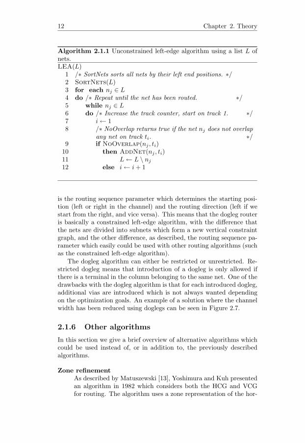
Algorithm 2.1.1 Unconstrained left-edge algorithm using a list L ofnets.LEA(L)
1 /∗ SortNets sorts all nets by their left end positions. ∗/2 SortNets(L)3 for each nj ∈ L4 do /∗ Repeat until the net has been routed. ∗/5 while nj ∈ L6 do /∗ Increase the track counter, start on track 1. ∗/7 i ← 18 /∗ NoOverlap returns true if the net nj does not overlap
any net on track ti. ∗/9 if NoOverlap(nj , ti)
10 then AddNet(nj , ti)11 L ← L \ nj
12 else i ← i + 1
is the routing sequence parameter which determines the starting posi-tion (left or right in the channel) and the routing direction (left if westart from the right, and vice versa). This means that the dogleg routeris basically a constrained left-edge algorithm, with the difference thatthe nets are divided into subnets which form a new vertical constraintgraph, and the other difference, as described, the routing sequence pa-rameter which easily could be used with other routing algorithms (suchas the constrained left-edge algorithm).
The dogleg algorithm can either be restricted or unrestricted. Re-stricted dogleg means that introduction of a dogleg is only allowed ifthere is a terminal in the column belonging to the same net. One of thedrawbacks with the dogleg algorithm is that for each introduced dogleg,additional vias are introduced which is not always wanted dependingon the optimization goals. An example of a solution where the channelwidth has been reduced using doglegs can be seen in Figure 2.7.
2.1.6 Other algorithms
In this section we give a brief overview of alternative algorithms whichcould be used instead of, or in addition to, the previously describedalgorithms.
Zone refinementAs described by Matuszewski [13], Yoshimura and Kuh presentedan algorithm in 1982 which considers both the HCG and VCGfor routing. The algorithm uses a zone representation of the hor-
2.1. Channel routing 13
Figure 2.5: Suboptimal solution from the constrained left-edge algo-rithm. Kernighan et al. [10].
Figure 2.6: A channel with a cyclic constraint and its correspondingVCG. Young Fung Yu [20].
izontal segments and merges nets in the VCG. The basic idea isto merge nets in the VCG and then all the merged nets in onenode should be placed on the same track. This algorithm doesnot handle unrestricted doglegs or vertical constraint cycles.
Linear time left edge, LTLEAZhang and Dai [21] presented an alternative solution of the left-edge algorithm which reduces the time complexity from O(n log n)to O(n). The experimental results show that for a large numberof nets, around 60.000, the running time is decreased by 99.7%.The authors also integrated the LTLEA with vertical constraints,without cyclic constraints. Compared to the constrained left-edge, using 5000 nets, the solutions are described to be similar,around 1.5% extra tracks are used in the LTLEA but the run-ning time is reduced with 98.5%. According to the authors allalgorithm variants that use LEA as base could be transformed to

14 Chapter 2. Theory
Figure 2.7: Reducing channel width using doglegs. Matuszewski [13].
LTLEA based algorithms.
Genetic algorithmsThere are many different variations of genetic algorithms (GA),that can be applied to the channel routing problem. A GA isan iterative procedure, a global evolutionary search technique,known to be efficient in the solution of NP-complete problems,see Davidenko et al. [5]. The GA processes a group of individu-als, which are a subset of possible solutions. The search criterionis called the fitness function, with which the GA estimates thequality of each individual. The GA applies different genetic op-erators on the population, such as crossover or mutation, with adefined probability to produce new individuals. In each iteration,new offspring is generated with the genetic operators. The pop-ulation size is kept constant by removing the least fit individualsaccording to the fitness function.
Gockel et al. [8] presented in 1996 a hybrid genetic algorithm forthe channel routing problem. It is called hybrid because a GAis combined with domain specific knowledge. This means thatthe initialization is made with a heuristic called ”random router”.The genetic operators used are cut, crossover and two mutationoperators that use a special technique called rip-up and reroute.Davidenko et al. [5] also presented a GA in 1996, but for thespecific case of restrictive channel routing, i.e. doglegs are notallowed. This algorithm uses information about horizontal andvertical constraints in the encoding of the individuals to earlyprevent illegal solutions. This leads to lower complexity and thesearch space is reduced. The experimental results show a maxi-mum deviation from optimum of 0.9% when using 66 nets. Theauthors conclude their report with a statement that the algorithmshows that domain specific knowledge greatly can improve GA

2.2. Graph searching 15
perfomance. This is also shown in the earlier described algorithmby Gockel et al. [8].
2.2 Graph searching
This section gives a brief introduction to graph searching and the Di-jkstra least-cost algorithm, which we will use in the implementation inChapter 4.
2.2.1 Definition
We start the definition of graph searching by defining a graph. A graphis a mathematical abstraction which is useful in problem solving. Agraph consists of a set of vertices, or nodes, and a set of edges. An edgeis a connection between two vertices. A graph can either be directedor undirected. In a directed graph, the edges are ordered pairs andconnect a source vertex to a target vertex. In the undirected graph,which we only will be considering further on, the edges are unorderedpairs. Describing an edge as {vi, vj}, a connection between vertex vi
and vj , is equal to {vj , vi}. Edges in a graph can also be associatedwith a weight, e.g. a length or a cost attribute. By introducing weightsto edges in a graph, the graph is called a weighted graph.
Graph searching is described by Lewis and Denenberg [12] as givena graph G and vertices v and w; the procedure of finding a path fromvertex v to w by recursively traversing edges to examine the verticesthat can be reached from v. We stop if we reach vertex w or if allvertices reachable from v has been examined. This procedure is calledgraph searching. The difference from searching the graph G and simplyiterating over all the vertices is that only a subset of all vertices arevisited. With this definition we continue describing some basic searchtechniques.
2.2.2 Depth-first search
The depth-first search technique, DFS, explores each vertex completelyas it is encountered, as described by Lewis and Denenberg [12]. Thismeans that if we start at v, first v is visited. Its first neighbor, v1,is encountered and visited. Then the first neighbor of v1 is explored,and so on. This procedure is called depth-first since it moves deeperafter every visit, and ”retreats” only if the vertex has no unexploredneighbors.
16 Chapter 2. Theory
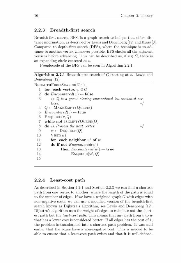
2.2.3 Breadth-first search
Breadth-first search, BFS, is a graph search technique that offers dis-tance information, as described by Lewis and Denenberg [12] and Biggs [3].Compared to depth first search (DFS), where the technique is to ad-vance to another vertex whenever possible, BFS checks all the adjacentvertices before advancing. This can be described as, if v ∈ G, there isan expanding circle centered at v.
Pseudocode of the BFS can be seen in Algorithm 2.2.1.
Algorithm 2.2.1 Breadth-first search of G starting at v. Lewis andDenenberg [12].BreadthFirstSearch(G, v)
1 for each vertex w ∈ G2 do Encountered(w) ← false3 /∗ Q is a queue storing encountered but unvisited ver-
tices. ∗/4 Q ← MakeEmptyQueue()5 Encountered(v) ← true6 Enqueue(v, Q)7 while not IsEmptyQueue(Q)8 do /∗ Process the next vertex. ∗/9 w ← Dequeue(Q)
10 Visit(w)11 for each neighbor w′ of w12 do if not Encountered(w′)13 then Encountered(w′) ← true14 Enqueue(w′, Q)15
2.2.4 Least-cost path
As described in Section 2.2.1 and Section 2.2.3 we can find a shortestpath from one vertex to another, where the length of the path is equalto the number of edges. If we have a weighted graph G with edges withnon-negative costs, we can use a modified version of the breadth-firstsearch known as Dijkstra’s algorithm, see Lewis and Denenberg [12].Dijkstra’s algorithm uses the weight of edges to calculate not the short-est path but the least-cost path. This means that any path from v to wthat has a lower cost is considered better. If all edges has the cost of 1,the problem is transformed into a shortest path problem. It was saidearlier that the edges have a non-negative cost. This is needed to beable to ensure that a least-cost path exists and that it is well-defined.

2.2. Graph searching 17
Pseudocode of the Dijkstra algorithm can be seen in Algorithm 2.2.2.The algorithm is a single source algorithm which finds the shortestpaths from vertex s ∈ G to all other vertices in G. This algorithmcan be modified to find the least-cost path between two vertices in thegraph just by setting a break condition if the desired vertex has beenfound.
Algorithm 2.2.2 Dijkstra’s algorithm for finding the distance betweena given source vertex s and all other vertices in the graph G. Lewisand Denenberg [12].DijkstraLeastCostPaths(G, s)
1 U ← MakeEmptySet()2 for each vertex v ∈ G3 do Distance(v) ←∞4 Insert(v, U)5 Distance(s) ← 06 while not IsEmpty(U)7 do v ← ExtractMin(U)8 Delete(v, U)9 for each neighbor w of v
10 do if Member(w, U)11 then totDist ← Distance(v) + Cost(v, w)12 Distance(w) ← min(Distance(w), totDist)13

18 Chapter 2. Theory
Chapter 3
Requirements
This chapter outlines the requirements for the project. The require-ments can be divided into three sections; topology modeling, optimiza-tion, and visualization.
3.1 Introduction
The main goal of this project is to develop a software demonstrator ofa concept tool to show the capabilities of methods to solve problemsin the layout process of FFC harnesses. To do so, we are required toinclude three major parts in the implementation. First, we need todefine the layout in an abstract unfolded view, a topology. Second,we need to route the nets to minimize the number of tracks and tomaximize cable usage. Third, the result from the routing should bepresented using a graphical representation.
3.2 Domain model
A domain model in Figure 3.1 shows the FFC harness and the channelrouting domains. As we can see, the FFC harness consists of both buscables, connector cables and connection matrices. The bus cable is thecable in which the nets are placed during routing, whereas the connectorcable is the cable that connects the connector to the bus cable. Eachbus can have multiple connection matrices which connect the bus toother buses or to connectors via connector cables. Each connector hasa set of pins in which the net numbers and width are defined. In theright part of Figure 3.1 we see the channel routing domain. A channelconsists of a set of terminals which form nets. The nets are placed onthe channel’s tracks. These are the two domains that we need to takeinto account during the implementation. As we will see in Chapter 4,
19
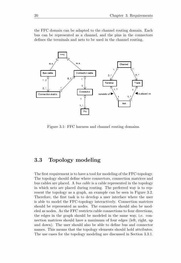
20 Chapter 3. Requirements
the FFC domain can be adapted to the channel routing domain. Eachbus can be represented as a channel, and the pins in the connectorsdefines the terminals and nets to be used in the channel routing.
Figure 3.1: FFC harness and channel routing domains.
3.3 Topology modeling
The first requirement is to have a tool for modeling of the FFC-topology.The topology should define where connectors, connection matrices andbus cables are placed. A bus cable is a cable represented in the topologyin which nets are placed during routing. The preferred way is to rep-resent the topology as a graph, an example can be seen in Figure 3.2.Therefore, the first task is to develop a user interface where the useris able to model the FFC-topology interactively. Connection matricesshould be represented as nodes. The connectors should also be mod-eled as nodes. As the FFC restricts cable connections to four directions,the edges in the graph should be modeled in the same way, i.e. con-nection matrices should have a maximum of four edges (left, right, upand down). The user should also be able to define bus and connectornames. This means that the topology elements should hold attributes.The use cases for the topology modeling are discussed in Section 3.3.1.

3.3. Topology modeling 21
Cm2
Cc2
Bus 1
C1
C2 C3
C4
Bus 1 Bus 1
Bus 2
Bus 2
Cm1 Cm3 Cm4
Cm5
Cm6
Cc1
Cc4
Cc3
C Connector
Cm Connection matrix
Cc Connector cable
Figure 3.2: Example of a FFC-topology with connection matrices, busesand connectors. Modified from Raithel [17].
3.3.1 Topology modeling use cases
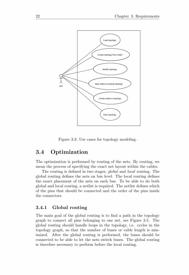
From the requirements specification by Raithel [16], use cases are de-veloped for the topology modeling. As seen in Figure 3.3, basic editorfunctionality is wanted. The user should be able to load, modify andsave the topology. More application specific requirements are the usecases that involve a netlist. A netlist is an input file which containsinformation about the connectors and the nets. The information in thenetlist defines the pins in each connector, the pin widths, and the netnumbers of the pins. It should be possible to create or modify topologyelements, in this case connectors, using the netlist. The use case tocreate a netlist from an existing topology is a secondary requirementwhich is only to be implemented if the basic requirements are fulfilled.
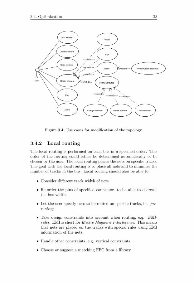
Figure 3.4 shows use cases for the topology modification. These aremainly standard editor requirements which should be implemented toguarantee basic functionality.
22 Chapter 3. Requirements
user
Modify topology
Create topology from netlist
Map netlist to existing topology
Create netlist in topology
Load topology
Save topology
Figure 3.3: Use cases for topology modeling.
3.4 Optimization
The optimization is performed by routing of the nets. By routing, wemean the process of specifying the exact net layout within the cables.
The routing is defined in two stages, global and local routing. Theglobal routing defines the nets on bus level. The local routing definesthe exact placement of the nets on each bus. To be able to do bothglobal and local routing, a netlist is required. The netlist defines whichof the pins that should be connected and the order of the pins insidethe connectors.
3.4.1 Global routing
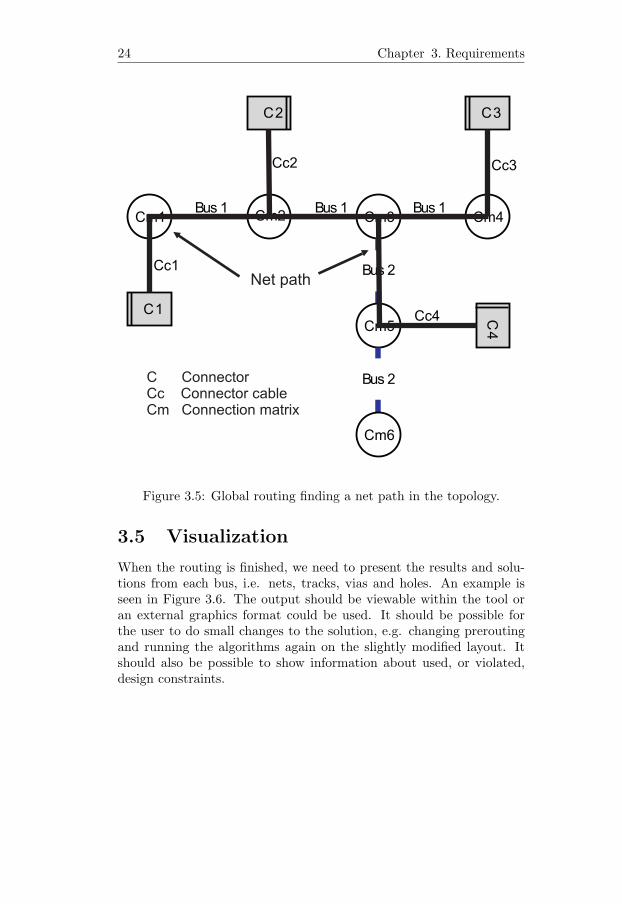
The main goal of the global routing is to find a path in the topologygraph to connect all pins belonging to one net, see Figure 3.5. Theglobal routing should handle loops in the topology, i.e. cycles in thetopology graph, so that the number of buses or cable length is min-imized. After the global routing is performed, the buses should beconnected to be able to let the nets switch buses. The global routingis therefore necessary to perform before the local routing.
3.4. Optimization 23
user
Add element
Delete element
Modify element
Rotate
Flip
Move
Modify attributes
Pan
Zoom Add attributeDelete attributeChange attribute
Copy element
Move multiple elements
<<extend>>
<<extend>>
<<extend>>
<<extend>>
<<extend>><<extend>><<extend>>
<<extend>>
Figure 3.4: Use cases for modification of the topology.
3.4.2 Local routing
The local routing is performed on each bus in a specified order. Thisorder of the routing could either be determined automatically or bechosen by the user. The local routing places the nets on specific tracks.The goal with the local routing is to place all nets and to minimize thenumber of tracks in the bus. Local routing should also be able to:
• Consider different track width of nets.
• Re-order the pins of specified connectors to be able to decreasethe bus width.
• Let the user specify nets to be routed on specific tracks, i.e. pre-routing.
• Take design constraints into account when routing, e.g. EMI-rules. EMI is short for Electro Magnetic Interference. This meansthat nets are placed on the tracks with special rules using EMIinformation of the nets.
• Handle other constraints, e.g. vertical constraints.
• Choose or suggest a matching FFC from a library.
24 Chapter 3. Requirements
Cm2
Cc2
Bus 1
C1
C2 C3C
4
Bus 1 Bus 1
Bus 2
Bus 2
Cm1 Cm3 Cm4
Cm5
Cm6
Cc1
Cc4
Cc3
C Connector
Cm Connection matrixCc Connector cable
Net path
Figure 3.5: Global routing finding a net path in the topology.
3.5 Visualization
When the routing is finished, we need to present the results and solu-tions from each bus, i.e. nets, tracks, vias and holes. An example isseen in Figure 3.6. The output should be viewable within the tool oran external graphics format could be used. It should be possible forthe user to do small changes to the solution, e.g. changing preroutingand running the algorithms again on the slightly modified layout. Itshould also be possible to show information about used, or violated,design constraints.

3.5. Visualization 25
Figure 3.6: Visualization example. Raithel [16].

26 Chapter 3. Requirements

Chapter 4
Implementation
This chapter describes how the three requirement parts were imple-mented. Topology modeling is described in Section 4.2. The opti-mization is split into global routing in Section 4.3 and local routing inSection 4.4. The connection between the global and local routing isdescribed in Section 4.5. The visualization is described in Section 4.6.The chapter is concluded with an overview class diagram of the imple-mentation in Section 4.8.
4.1 Previous work
The previous application, described in Section 1.3, was ported to Javafrom its current implementation in C++. By doing this, we have aJava implementation of the left-edge algorithm which could be usedand extended if necessary. The genetic algorithm which was used tooptimize the pin order was not ported because of new requirements.The limitation of this application is that it can only handle local routingon one bus at a time. The inputs, the top and bottom terminals, aredefined in text files and the output is also stored in text files along witha SVG, see Appendix A, solution.
4.2 Topology modeling
This section describes the implementation and functionality of the topol-ogy modeling. The limitations and the use of attributes are describedin Section 4.2.3 and Section 4.2.4 respectively.
27

28 Chapter 4. Implementation
4.2.1 Introduction
Prior to any implementation, research was conducted to be able to finda suitable framework for graph modeling and visualization. The choicefell on the Java toolkit JGraph, see Alder [2], since it is a very well doc-umented and widely used framework. There has been several, commer-cial and non-commercial, applications developed using this framework.The most important motivation why this framework was chosen wasbecause it was free and open-source. Since the framework is writtenusing Java, Java was used to build the application.
The topology modeling requirement has been implemented as agraph layout editor using the JGraph framework. Real world elementsare represented by graph elements, see Figure 4.1. Connection matricesand connectors are represented as nodes, and bus cable segments andconnector cables are represented as edges in the graph. Connector ori-entations are recognized by a black stripe which indicates the positionof pin number one inside the connector. Using these graph elements,we can model FFC harnesses in the editor. A screenshot of the editoralong with a modeled harness can be seen in Figure 4.2. In this picturewe see the major sections of the application layout. We have menusand a toolbar at the top providing functionality, described more in Sec-tion 4.2.2. To the right is the graph editor area in which the topologyis modeled using the elements described in Figure 4.1. To the left isthe netlist view in which connector names are displayed after a XMLnetlist has been imported.
Figure 4.1: Representation of real world elements in the topology.

4.2. Topology modeling 29
Figure 4.2: Screenshot of the implemented editor with a modeled FFCharness.
4.2.2 Functionality
This section gives a description of the functionality within the editorand explanations of how they were implemented. The functionality ispresented in each of the use cases for the topology modeling.
Load and save topologyThe Java XMLEncoder and XMLDecoder class has been used toallow saving and loading of topologies in the editor. Since theXML classes only read and write Java Bean properties, imagesare not supported. Additional code has been written to allowimages in the graph, in our case the connector images.
Create topology from netlistIf a netlist is imported, connector names are displayed in a listto allow creation of connector elements in the layout. The con-nector names in the list are drag-and-drop enabled which meansthat the names can be dragged into the layout to create connectorelements. The netlist is defined in a custom XML format whichcontains information about connectors, pins, and nets. The XMLformat for the netlist was chosen because it provides a structured
30 Chapter 4. Implementation
way of storing information, and we can easily use Java XML de-coder and encoder classes to read the files. The XML netlistformat is just one example how a real netlist could look like. Ifother formats are used for the netlist, the classes that handle thenetlist loading can easily be replaced. An example of a netlist isseen in Appendix B.
Map netlist to existing topologyExisting connector elements in the topology can be modified bydropping a connector name from the list on top of them.
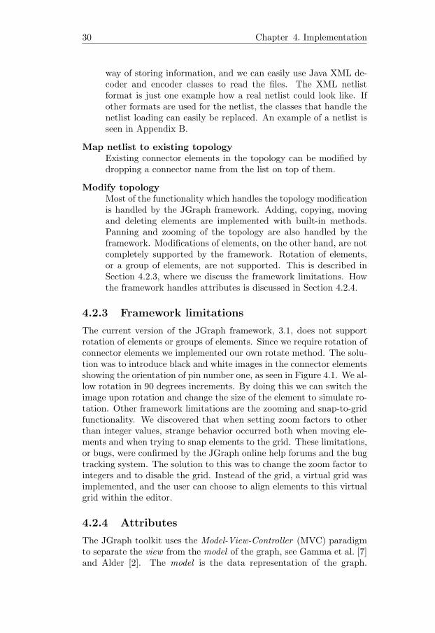
Modify topologyMost of the functionality which handles the topology modificationis handled by the JGraph framework. Adding, copying, movingand deleting elements are implemented with built-in methods.Panning and zooming of the topology are also handled by theframework. Modifications of elements, on the other hand, are notcompletely supported by the framework. Rotation of elements,or a group of elements, are not supported. This is described inSection 4.2.3, where we discuss the framework limitations. Howthe framework handles attributes is discussed in Section 4.2.4.
4.2.3 Framework limitations
The current version of the JGraph framework, 3.1, does not supportrotation of elements or groups of elements. Since we require rotation ofconnector elements we implemented our own rotate method. The solu-tion was to introduce black and white images in the connector elementsshowing the orientation of pin number one, as seen in Figure 4.1. We al-low rotation in 90 degrees increments. By doing this we can switch theimage upon rotation and change the size of the element to simulate ro-tation. Other framework limitations are the zooming and snap-to-gridfunctionality. We discovered that when setting zoom factors to otherthan integer values, strange behavior occurred both when moving ele-ments and when trying to snap elements to the grid. These limitations,or bugs, were confirmed by the JGraph online help forums and the bugtracking system. The solution to this was to change the zoom factor tointegers and to disable the grid. Instead of the grid, a virtual grid wasimplemented, and the user can choose to align elements to this virtualgrid within the editor.
4.2.4 Attributes
The JGraph toolkit uses the Model-View-Controller (MVC) paradigmto separate the view from the model of the graph, see Gamma et al. [7]and Alder [2]. The model is the data representation of the graph.

4.3. Global routing 31
The model holds only connectivity information, also known as graphstructure, and not geometric information. If the model changes, allviews connected to the model get an opportunity to update themselves.This allows to attach multiple views, with different representations, toone model, see Figure 4.3.
Figure 4.3: Model-View-Controller (MVC). Alder [2].
We have introduced custom attributes to the elements in the topol-ogy, in the model. We have type attributes which are set upon in-sertion. The type attribute determines if the element is a connectionmatrix, connector, bus or connection line. We also have attributes onthe connector elements to determine the orientation. The connectorsand the buses have name attributes which can be modified by the userand length attributes on buses and connection lines. The use cases forthe topology modification in Figure 3.4 describes adding and deletingattributes. This is not implemented. The attributes in the editor cannot be removed and new custom attributes can not be added. How-ever, this behavior could be implemented in the future just as we haveimplemented the previously described attributes.
4.3 Global routing
This section describes the global routing problem and how it was solved.
32 Chapter 4. Implementation
4.3.1 Introduction
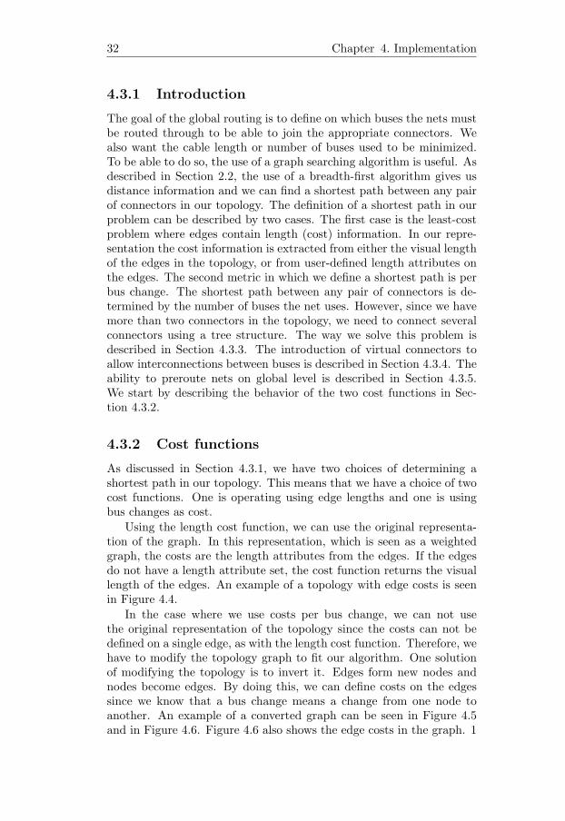
The goal of the global routing is to define on which buses the nets mustbe routed through to be able to join the appropriate connectors. Wealso want the cable length or number of buses used to be minimized.To be able to do so, the use of a graph searching algorithm is useful. Asdescribed in Section 2.2, the use of a breadth-first algorithm gives usdistance information and we can find a shortest path between any pairof connectors in our topology. The definition of a shortest path in ourproblem can be described by two cases. The first case is the least-costproblem where edges contain length (cost) information. In our repre-sentation the cost information is extracted from either the visual lengthof the edges in the topology, or from user-defined length attributes onthe edges. The second metric in which we define a shortest path is perbus change. The shortest path between any pair of connectors is de-termined by the number of buses the net uses. However, since we havemore than two connectors in the topology, we need to connect severalconnectors using a tree structure. The way we solve this problem isdescribed in Section 4.3.3. The introduction of virtual connectors toallow interconnections between buses is described in Section 4.3.4. Theability to preroute nets on global level is described in Section 4.3.5.We start by describing the behavior of the two cost functions in Sec-tion 4.3.2.
4.3.2 Cost functions
As discussed in Section 4.3.1, we have two choices of determining ashortest path in our topology. This means that we have a choice of twocost functions. One is operating using edge lengths and one is usingbus changes as cost.
Using the length cost function, we can use the original representa-tion of the graph. In this representation, which is seen as a weightedgraph, the costs are the length attributes from the edges. If the edgesdo not have a length attribute set, the cost function returns the visuallength of the edges. An example of a topology with edge costs is seenin Figure 4.4.
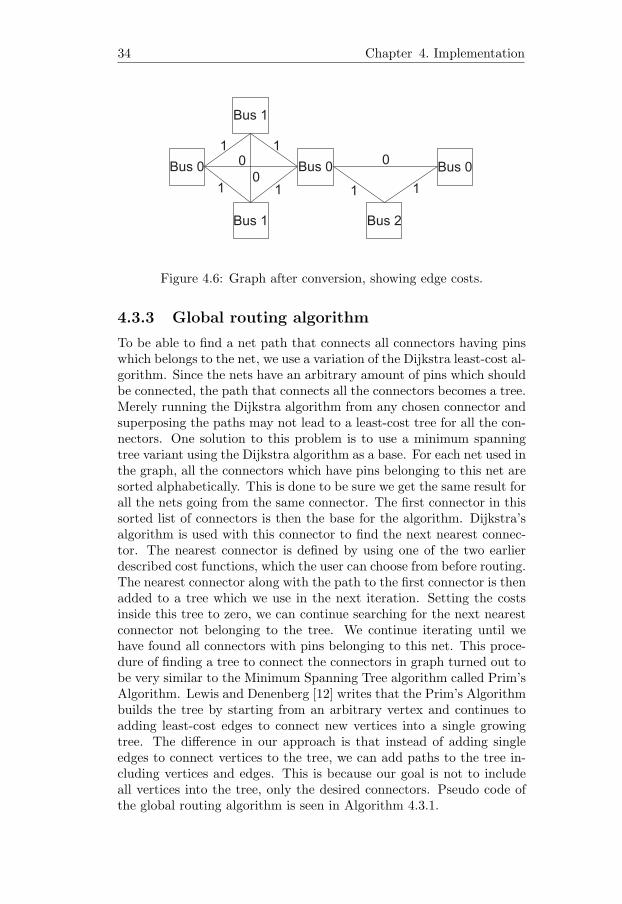
In the case where we use costs per bus change, we can not usethe original representation of the topology since the costs can not bedefined on a single edge, as with the length cost function. Therefore, wehave to modify the topology graph to fit our algorithm. One solutionof modifying the topology is to invert it. Edges form new nodes andnodes become edges. By doing this, we can define costs on the edgessince we know that a bus change means a change from one node toanother. An example of a converted graph can be seen in Figure 4.5and in Figure 4.6. Figure 4.6 also shows the edge costs in the graph. 1

4.3. Global routing 33
Figure 4.4: Topology graph with edge costs.
for bus change, and 0 for edges on the same bus. After the inversion,we can apply the algorithm in Algorithm 4.3.1 in the same manner aswith the length cost function.
Figure 4.5: Topology graph in the original representation.
34 Chapter 4. Implementation
Figure 4.6: Graph after conversion, showing edge costs.
4.3.3 Global routing algorithm
To be able to find a net path that connects all connectors having pinswhich belongs to the net, we use a variation of the Dijkstra least-cost al-gorithm. Since the nets have an arbitrary amount of pins which shouldbe connected, the path that connects all the connectors becomes a tree.Merely running the Dijkstra algorithm from any chosen connector andsuperposing the paths may not lead to a least-cost tree for all the con-nectors. One solution to this problem is to use a minimum spanningtree variant using the Dijkstra algorithm as a base. For each net used inthe graph, all the connectors which have pins belonging to this net aresorted alphabetically. This is done to be sure we get the same result forall the nets going from the same connector. The first connector in thissorted list of connectors is then the base for the algorithm. Dijkstra’salgorithm is used with this connector to find the next nearest connec-tor. The nearest connector is defined by using one of the two earlierdescribed cost functions, which the user can choose from before routing.The nearest connector along with the path to the first connector is thenadded to a tree which we use in the next iteration. Setting the costsinside this tree to zero, we can continue searching for the next nearestconnector not belonging to the tree. We continue iterating until wehave found all connectors with pins belonging to this net. This proce-dure of finding a tree to connect the connectors in graph turned out tobe very similar to the Minimum Spanning Tree algorithm called Prim’sAlgorithm. Lewis and Denenberg [12] writes that the Prim’s Algorithmbuilds the tree by starting from an arbitrary vertex and continues toadding least-cost edges to connect new vertices into a single growingtree. The difference in our approach is that instead of adding singleedges to connect vertices to the tree, we can add paths to the tree in-cluding vertices and edges. This is because our goal is not to includeall vertices into the tree, only the desired connectors. Pseudo code ofthe global routing algorithm is seen in Algorithm 4.3.1.

4.3. Global routing 35
Algorithm 4.3.1 The global routing algorithm. L is a list of all thenets used in the topology graph G.Global routing algorithm(G,L)
1 for each ni ∈ L2 do T ← ∅3 SortConnectors(ni)4 for each cj ∈ ni
5 do /∗ FindNearestConnector uses the Dijkstra algorithm tofind the path to the next nearest connector. ∗/
6 path ← FindNearestConnector()7 /∗ Add the path to the tree and update the costs. ∗/8 AddPath(T, path)9 UpdateCosts(T )
4.3.4 Virtual connectors
The goal with the global routing was to make sure that connectors withpins that belong to the same net are connected. We use the informationgathered in the global routing phase and introduce virtual connectors.During the global routing phase, the virtual connectors are created onthe buses that have nets that change buses. The creation works asfollows. In the global routing algorithm, after the path to the nextnearest bus or connector has been found, the path is traversed to seeif any bus changes occur. If we notice a bus change, we know that weshould add a virtual connector or a pin to an already existing virtualconnector. The virtual connector name is based on the two buses thatit connects. If we are going from bus 1 to bus 2, the virtual connectoris named BUS1-BUS2. This name is later used by the topology parsingand the left-edge algorithm which was described in Section 4.4.2.
The pin we add has the same net number as the net we are runningthe algorithm on. To determine the width of the virtual connector’spin, we add the largest pin width of all this net’s pins. This is made tomake sure that we do not use a smaller width than allowed.
The use and behavior of the virtual connectors are described furtherin Section 4.5.
4.3.5 Global prerouting
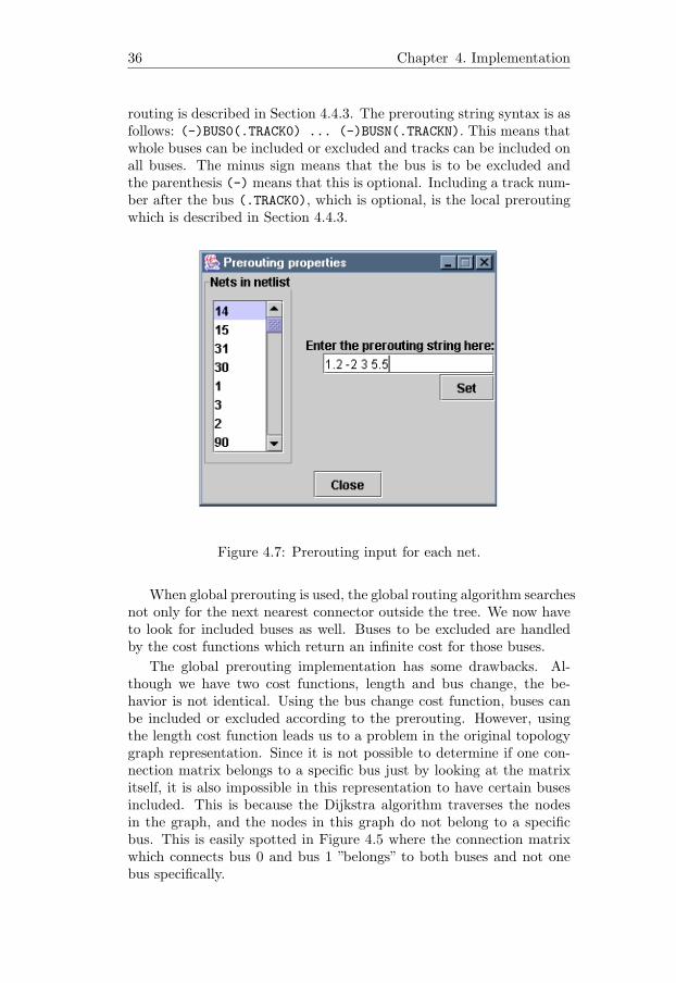
Global prerouting has been implemented to let the user define a netpath on bus level. This means that the user can include and excludebuses for each net. The prerouting is made via a prerouting stringwhich the user can enter for each net, see Figure 4.7. This preroutingstring defines prerouting on both global and local level. The local pre-
36 Chapter 4. Implementation
routing is described in Section 4.4.3. The prerouting string syntax is asfollows: (-)BUS0(.TRACK0) ... (-)BUSN(.TRACKN). This means thatwhole buses can be included or excluded and tracks can be included onall buses. The minus sign means that the bus is to be excluded andthe parenthesis (-) means that this is optional. Including a track num-ber after the bus (.TRACK0), which is optional, is the local preroutingwhich is described in Section 4.4.3.
Figure 4.7: Prerouting input for each net.
When global prerouting is used, the global routing algorithm searchesnot only for the next nearest connector outside the tree. We now haveto look for included buses as well. Buses to be excluded are handledby the cost functions which return an infinite cost for those buses.
The global prerouting implementation has some drawbacks. Al-though we have two cost functions, length and bus change, the be-havior is not identical. Using the bus change cost function, buses canbe included or excluded according to the prerouting. However, usingthe length cost function leads us to a problem in the original topologygraph representation. Since it is not possible to determine if one con-nection matrix belongs to a specific bus just by looking at the matrixitself, it is also impossible in this representation to have certain busesincluded. This is because the Dijkstra algorithm traverses the nodesin the graph, and the nodes in this graph do not belong to a specificbus. This is easily spotted in Figure 4.5 where the connection matrixwhich connects bus 0 and bus 1 ”belongs” to both buses and not onebus specifically.

4.4. Local routing 37
4.4 Local routing
In this section the local routing is explained and how concepts fromthe VLSI channel routing can be adapted to our problem. We describehow the topology is validated and translated into a representation thatcan be used by the local routing. We also describe local prerouting andcable type selection which affects the local routing behavior.
4.4.1 Channel routing
As we have described in Chapter 2, the VLSI channel routing problembasically consists of two rows of terminals. There is one row at the topand one row at the bottom of the channel. The terminals with samenumbers are connected inside the channel on the tracks and form nets.In our topology representation, each bus cable becomes a channel. Theconnectors on the bus, or other buses that are connected via virtual con-nectors, consist of pins with net numbers which becomes the terminalswhich should be connected. The pins and their net numbers are definedin the netlist which is loaded within the editor. A netlist example canbe seen in Appendix B. The basic approach to the channel routingproblem is to solve it with the left-edge algorithm, also described inChapter 2. This algorithm is also the base of our operations.
In Figure 4.8, we can see a bus cable to the left with four connectorsand their pins. The net numbers of the pins are displayed at the topand bottom. The channel routing representation of the bus is shown tothe right and a solution using the left-edge algorithm is shown to thebottom right. The solution determines the placement of the vias in thebus and if there should be any holes in the cable in the case nets sharethe same track.

38 Chapter 4. Implementation
Figure 4.8: The channel routing representation of a bus cable and asolution with the left-edge algorithm.
The original left-edge algorithm does not handle different trackwidths. In VLSI design, the tracks in the channel have no specifiedwidth. In our problem, all pins can have different width and thereforethe tracks shall match the widths of the nets. The width is determinedby the width attribute of the pins in the netlist. The left-edge algo-rithm has been modified to assign widths to the tracks using this pinattribute. There has been additional modifications to the left-edge al-gorithm, as prerouting and cable type selection. These modificationsare described more in detail in Section 4.4.3 and Section 4.4.4.
To be able to use our modeled topology, we need to translate thetopology to a representation that can be handled by the left-edge algo-rithm. We continue by describing the methods of parsing the topologyand how we validate it.
4.4.2 Topology parsing and validation
The topology needs to be parsed and validated before we can do anylocal routing. The topology is represented as a tree in the model andwe can traverse the tree to find the information we need. What we needto find out, for each bus, is which connectors and buses are connectedto it, and the position and orientation of the connectors. With helpfrom the orientation attribute of the connectors, we can read this fromthe elements in the topology. In general, the procedure of getting in-formation from one bus works as follows. First, we need to find a startor end node of this bus to determine the start position of the parsing.This is done by searching elements in the graph until we find a bus line

4.4. Local routing 39
which belongs to this bus. The nodes, the connection matrices, on thisedge are parsed and if one of the nodes only has one edge connectedwhich belongs to this bus, this is a start or end node. By knowing thestart node for our parsing, we can also check the direction of the bus,horizontal or vertical. This is done by looking at the connection port onthe node element. The connection port is the area on the node elementwhere the edge is connected in the topology. We can now parse eachnode on the bus by traversing the topology graph and look for connec-tors or other buses. The connector names are added to the bus objectwhich is used by the left edge algorithm to get the top and bottom pinrows for the routing.
If we find a connected bus, we should add the name of the virtualconnector which is top-BUS1-BUS2 or bottom-BUS1-BUS2. BUS1 isthe current bus and BUS2 is the connected bus and top or bottomdetermines if the virtual connector is added to the top or at the bottomof the bus cable. The usage of top and bottom virtual connectors isto gain control of the via placement in the connection matrices, seeSection 4.5.
During the parsing, we also validate the graph to make sure thetopology is valid. We have introduced constraints on the topology toavoid situations which make it invalid and unroutable. These con-straints are introduced due to either real design and manufacturingconstraints, or because the cases are not handled in the implementa-tion of the algorithms. The constraints which make the topology graphinvalid are:
Bus constraintsBuses are not allowed to change direction. A bus must be ei-ther horizontal or vertical. All buses must have their own uniqueidentifier to be able to parse the topology correctly.
Connection constraintsA connection matrix must hold a maximum of one connector.This is to avoid vertical constraints and to avoid differences inthe pin count on the top and bottom arrays. A connection matrixis only allowed to have one bus and connector, or two buses andno connector. This is to make sure the connector is connected onone bus only.
Connector constraintsConnectors must not be modeled at the end of a bus. Connectorsmust be either on the top or bottom. Connector orientation mustbe aligned with the bus to determine the correct position of pinnumber one. This means that a connector must run in parallelwith the bus. The correct connector port must be used when
40 Chapter 4. Implementation
connected to a bus. E.g. if a connector is modeled at the top ofthe bus, the bottom port of the connector must be used.
If the topology is invalidated during the parsing, the user is givenan error message describing the errors in the topology and the globaland local routing is aborted.
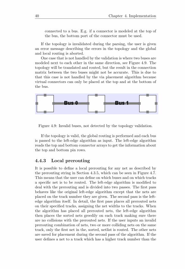
One case that is not handled by the validation is where two buses aremodeled next to each other in the same direction, see Figure 4.9. Thetopology will be translated and routed, but the result in the connectionmatrix between the two buses might not be accurate. This is due tothat this case is not handled by the via placement algorithm becausevirtual connectors can only be placed at the top and at the bottom ofthe bus.
Figure 4.9: Invalid buses, not detected by the topology validation.
If the topology is valid, the global routing is performed and each busis passed to the left-edge algorithm as input. The left-edge algorithmreads the top and bottom connector arrays to get the information aboutthe top and bottom pin rows.
4.4.3 Local prerouting
It is possible to define a local prerouting for any net as described bythe prerouting string in Section 4.3.5, which can be seen in Figure 4.7.This means that the user can define on which buses and on which tracksa specific net is to be routed. The left-edge algorithm is modified todeal with the prerouting and is divided into two passes. The first passbehaves like the original left-edge algorithm except that the nets areplaced on the track number they are given. The second pass is the left-edge algorithm itself. In detail, the first pass places all prerouted netson their specified tracks, assigning the net widths to the tracks. Whenthe algorithm has placed all prerouted nets, the left-edge algorithmthen places the sorted nets greedily on each track making sure thereare no collisions with the prerouted nets. If the user inputs an invalidprerouting combination of nets, two or more colliding nets on the sametrack, only the first net in the, sorted, netlist is routed. The other netsare saved for placement during the second pass of the algorithm. If theuser defines a net to a track which has a higher track number than the

4.4. Local routing 41
optimal channel width, extra tracks with zero width are introduced tomake sure that the net is routed on the user specified track.
Using local prerouting to exclude nets from tracks is no requirementand is not implemented.
4.4.4 Cable type selection
The user is given the possibility to assign a specific cable to each busin the topology, see Figure 4.10.
Figure 4.10: Possibility to assign an FFC cable to a bus. Here with thecable library from Appendix C.
The cables are defined in an XML file,very similar to the netlist spec-ification. An example of a cable library can be seen in Appendix C. Thecable library defines the amount of tracks in the cable, and the widthsfor each track. The ability to specify cable types to buses introducesnew constraints to the left-edge algorithm. If a net can not be routedon the specified cable we must violate one of the constraints. The tracknumber constraint or the track width constraint must be overridden.It is decided that if a cable type is specified, the track widths in thecable shall stay intact. This is because that if a net is routed on atrack with smaller width than the net itself, this will most likely leadto an overload/overheat in the cable. Instead, we can violate the tracknumber constraint to introduce new tracks to make sure that the netis routed properly.
The new constraints with the track widths also imply that we can

42 Chapter 4. Implementation
not use the standard greedy placing algorithm. We also do not know ifwe are guaranteed an optimum solution as with the standard left-edgealgorithm. The new modifications to the algorithm are as follows. Weinitialize all tracks with their new width according to the specificationof the cable. If we have local prerouting, the cable information is used tospecify the widths, and we have to check if the widths of the preroutednets match the widths of the tracks. If the prerouted net does not fit onthe specified tracks, it is saved until the second pass of the algorithm.During the second pass, we can not place the nets greedily on the tracksas before since we have the width attribute to take into account. Forevery net, the smallest track, where the net fits, is located. If the netdoes not fit on any other, smaller, track, the net is routed on the currenttrack.
If nets can not fit within the specified cable, additional tracks haveto be added to make sure the nets are routed. The constraints thatare violated are displayed for each bus in the report files, described inSection 4.6.
4.5 Via placement
As we have mentioned earlier in Section 4.3.4 the introduction of vir-tual connectors makes it possible for nets to use more than one bus.During the implementation phase, we used the virtual connectors as asolution to the problem, but did not think of the via configuration thatappeared in the connection matrices between the buses. The pins inthe virtual connectors are added in the order the nets are routed butthis order was never changed. What was discovered was that the viaconfigurations in the connection matrices between the buses did notmatch. This means that we only had information about the nets, butnot the via placements. This problem is seen in Figure 4.11 where thefirst version of the introduced virtual connectors is seen. Two buses,BUS0 and BUS1, are connected using a virtual connector named 1-0.The connection matrix displayed on both buses is supposed to have thesame via placement on both buses, since it is the same matrix. As wesee in the connection matrix, the via placement does not match. Alsonotice that all virtual connectors are equally configured and have thesame name (1-0).
To deal with the via placement problem the behavior of the virtualconnectors was improved. First, top and bottom virtual connectorswere introduced, as described in Section 4.4.2. The use of top andbottom virtual connectors makes it possible to gain control over thebehavior of the pin order inside the connectors. Changing order of thepins affects both the via placement and the routability. If we changethe pin order of connectors, the layout might not be routable. On a

4.5. Via placement 43
Figure 4.11: Connection matrices with incorrect via placement.
bus, virtual connectors could be placed so that we introduce verticalconstraints, i.e. opposing pins/terminals in the same row. Since theleft-edge algorithm does not take this into account, the solution mightnot be feasible. However, the vertical constraints are reported alongwith the other violated constraints in the report files.
If we look at Figure 4.11 again, the nets 1, 2 and 3 are used onboth buses. These three nets are the nets that should be used insidethe connection matrix with help from the virtual connectors. There aretwo problems; The via placement is incorrect and net number 2 seemsto be going both left and right according to the connection matrix inBUS1. What we do to solve the via placement problem is to updatethe virtual connectors pin order after each bus has been routed and tolook at the direction of the routed nets. To be able to have a correctpin order on the connectors on BUS1, we need to look at the order ofnets on the tracks they are routed on, i.e. BUS0 the first bus. However,the direction of the nets on BUS0 influences the pin configuration inthe connectors. This is where the use of the top and bottom distinctioncomes in. The nets going left are added to the top virtual connectoron BUS1 and the nets going right are added to the bottom virtualconnector. Since one connector is having 3 nets, the other 2, a new pinwith net number 0 is inserted on one connector. Net number 0 means

44 Chapter 4. Implementation
that no net is connected. This introduction is made to make sure thepin count on both connectors match and to make sure the pins areplaced on the correct position in the connector.
Now, there are two, correctly, configured virtual connectors forBUS1 which match BUS0. This bus can now be routed. The prob-lem is now that the pin order on the virtual connector on BUS0 mightnot be consistent with the new net order on BUS1. We have to re-configure the virtual connector, using the same technique as above, tomatch the net order on BUS1, and reroute BUS0. The pin order on thevirtual connectors, and the net order on the tracks on the buses shouldnow match.
Still, the via placements inside the connection matrix are not guar-anteed to be valid. Since the bus is rerouted, the solution might change,i.e. if the net order on the tracks changes. If the solution changes, thevia placement becomes incorrect. To prevent this, we can use the earlierdescribed prerouting to ”lock” the solution after routing. This meansthat when the bus is routed the second time, we are using the sametracks for the nets as in the first solution. A valid solution, with theuse of top and bottom connectors, is displayed in Figure 4.12.
Figure 4.12: Connection matrices with correct via placement.
4.6. Visualization 45
4.6 Visualization
The visualization is realized with the Scalable Vector Graphics, SVG,format, see Appendix A. This format has been used in the tool withhelp from the Batik library for Java, see Appendix A. The Batik li-brary provides methods for creating and manipulating SVG output.The SVG format also makes it possible for easy enhancement and in-teractivity in the produced output. The output could be integrated intothe application, or as in this project, integrated in an HTML document.
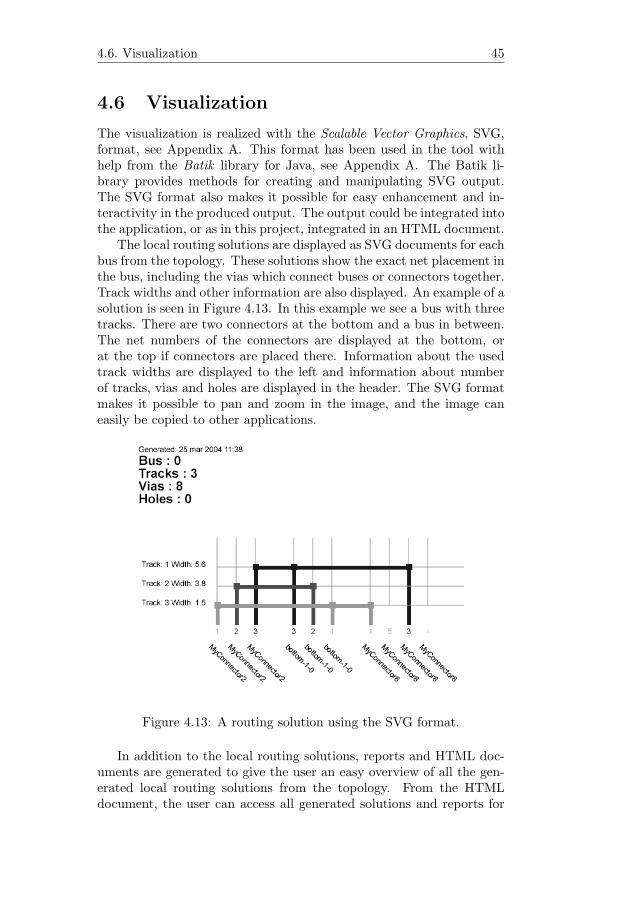
The local routing solutions are displayed as SVG documents for eachbus from the topology. These solutions show the exact net placement inthe bus, including the vias which connect buses or connectors together.Track widths and other information are also displayed. An example of asolution is seen in Figure 4.13. In this example we see a bus with threetracks. There are two connectors at the bottom and a bus in between.The net numbers of the connectors are displayed at the bottom, orat the top if connectors are placed there. Information about the usedtrack widths are displayed to the left and information about numberof tracks, vias and holes are displayed in the header. The SVG formatmakes it possible to pan and zoom in the image, and the image caneasily be copied to other applications.
Figure 4.13: A routing solution using the SVG format.
In addition to the local routing solutions, reports and HTML doc-uments are generated to give the user an easy overview of all the gen-erated local routing solutions from the topology. From the HTMLdocument, the user can access all generated solutions and reports for
46 Chapter 4. Implementation
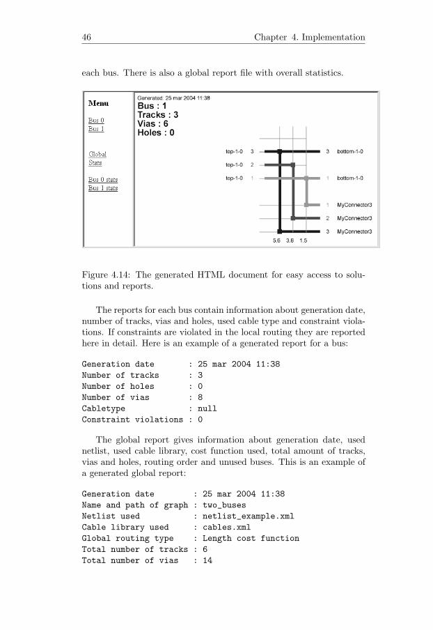
each bus. There is also a global report file with overall statistics.
Figure 4.14: The generated HTML document for easy access to solu-tions and reports.
The reports for each bus contain information about generation date,number of tracks, vias and holes, used cable type and constraint viola-tions. If constraints are violated in the local routing they are reportedhere in detail. Here is an example of a generated report for a bus:
Generation date : 25 mar 2004 11:38Number of tracks : 3Number of holes : 0Number of vias : 8Cabletype : nullConstraint violations : 0
The global report gives information about generation date, usednetlist, used cable library, cost function used, total amount of tracks,vias and holes, routing order and unused buses. This is an example ofa generated global report:
Generation date : 25 mar 2004 11:38Name and path of graph : two_busesNetlist used : netlist_example.xmlCable library used : cables.xmlGlobal routing type : Length cost functionTotal number of tracks : 6Total number of vias : 14
4.7. Application examples 47
Total number of holes : 0Total number of buses : 2Bus routing order : 0 1Buses not used :
4.7 Application examples
To show the capabilities of the tool, the cockpit example from Figure 1.4has been modeled with the tool. The topology consists of one bus andconnectors connected to it on one side. An XML netlist was producedaccording to real connector specifications from the cockpit harness. Thenetlist was imported to the application and together with the topology,a local routing solution was produced.
On the following pages are examples from the application presented.The cockpit example from Figure 1.4 is modeled and shown in Fig-ure 4.15. An excerpt from the local routing solution of this example isseen in Figure 4.16 and an overview of the whole local routing solutionin Figure 4.17.
4.8 Class overview
To conclude this chapter, a class diagram in Figure 4.18 presents themajor classes and the most important relations. Minor GUI classesand action classes are left out for readability reasons. This class di-agram is intended to give an overview of the application design. Asseen, the editor is the main class which creates handlers upon creation.The different handlers takes care of e.g. the loading and saving ofgraphs, netlist and cablelist import and solution output. When loadinga netlist, connector, net and pin instances are created which are usedin the routing by the Lea class. The GraphHandler class handles theparsing of the editor layout, the global routing and upon routing thisclass creates a bus with connectors which the Lea class can access.
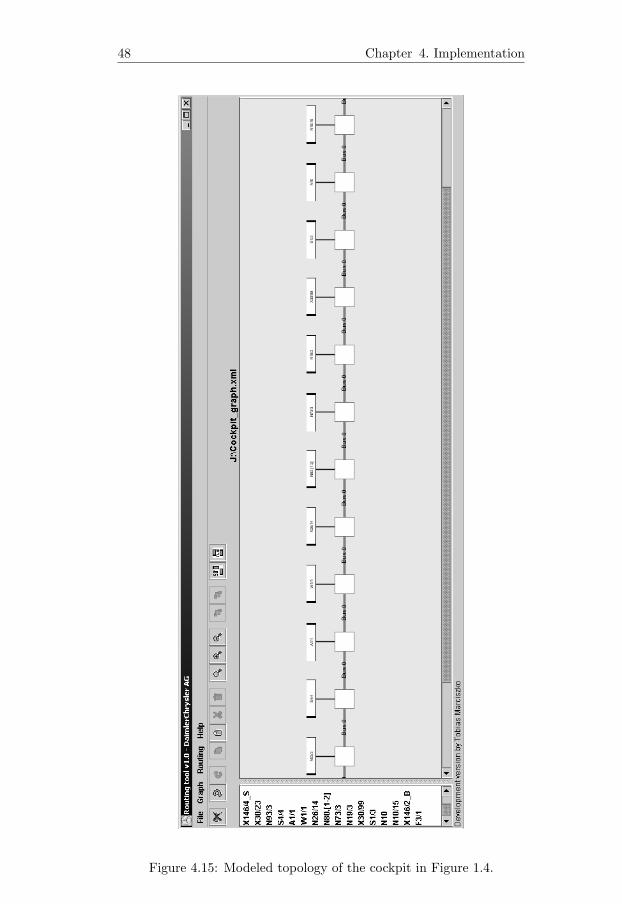
48 Chapter 4. Implementation
Figure 4.15: Modeled topology of the cockpit in Figure 1.4.

4.8. Class overview 49
Figure 4.16: Excerpt from the local routing solution of the cockpit inFigure 1.4.
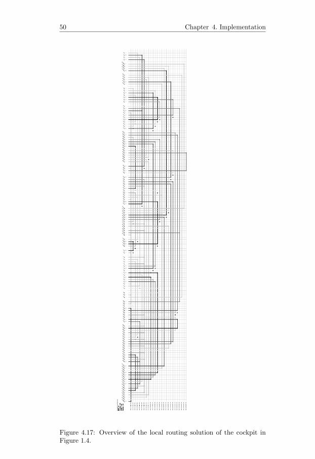
50 Chapter 4. Implementation
Figure 4.17: Overview of the local routing solution of the cockpit inFigure 1.4.

4.8. Class overview 51
Figure 4.18: Overview of the main classes in the application.

52 Chapter 4. Implementation

Chapter 5
Summary
A software demonstrator of a concept tool for layout and optimizationof flat cable layouts has been developed. The tool has been written us-ing Java along with the JGraph and Batik frameworks. The Java imple-mentation facilitates the use of the application on several platforms andthe application can easily be extended using the chosen frameworks.
According to the requirements, the tool handles topology modelingof FFC layouts using graph elements to represent real world elements.The graph elements in the editor can be added and modified. Importinga netlist to the application makes it possible to insert connectors usingdrag and drop. Existing connectors can also be modified using dragand drop. Graph layouts can be saved and loaded in the application.The extra requirement to create a netlist from the topology was notprioritized and not implemented.
The topology modeling handles the basic aspects of FFC layouting.However, constraints have been introduced in the layout to prevent theuser from modeling unsupported topologies. These constraints can beremoved to fit future requirements and to extend the current featuresof the tool. The most significant constraint is that connectors in thetopology are not allowed to be modeled on the same connection matrix.This is to avoid vertical constraints which is not supported by theimplemented routing algorithms.
Optimization of the layout has been divided into two stages as sug-gested by the requirements. The developed global routing algorithmuses an implementation and extension of the Dijkstra algorithm to buildtrees of connectors in the topology. To be able to connect the busestogether using connection matrices, we introduced a concept called vir-tual connectors to make sure the nets can be routed over more than onebus. These virtual connectors are used by the local routing. The globalrouting uses two types of cost functions, length or bus change, to deter-mine a least-cost path in the topology. To be able to gain control of the
53

54 Chapter 5. Summary
behavior of the global routing, global prerouting has been introduced.The global prerouting allows the user to influence the path of the net.However, since the two cost functions use two different representationsof the topology, the user is not able to include buses using the lengthcost function. Using the bus change cost function allows both inclusionand exclusion of buses to the prerouting.
The local routing is based on the left-edge algorithm taken from theVLSI channel routing. The algorithm is extended to take track widthsinto account to be able to match the net widths to the tracks in thebus. The left-edge algorithm implementation from Fritz [6] was usedand ported to Java. Further enhancements to the left-edge algorithmand local routing is the local prerouting and cable type selection. Thelocal prerouting grants the user the possibility to specify tracks forthe nets. The cable type selection defines the number of tracks andtrack widths of a bus. The left-edge algorithm was modified to handleprerouting and cable type selection together.
A method to configure the connection matrices was needed andalso developed. The proposed idea to use virtual connectors makesit possible to gain control over via placement inside the connectionmatrices. This method arranges the virtual connectors’ pin order tomatch the net order on the previously routed bus and gives feasiblesolutions. However, the method could produce vertical constraints insome hard cases. Using prerouting on both global and local level givesthe user more control over the behavior to avoid vertical constraints.
The visualization of the result is implemented with HTML docu-ments and local routing solutions in the SVG format. The local rout-ing solutions are collected in the HTML document which provides anoverview along with report files for each routed bus and overall statis-tics.
The application demonstrates the basic concepts of the design andoptimization of the flexible flat cable layouts. Most of the requirementssuggested by Raithel [16] has been implemented and the applicationshows that the methods developed here can be further enhanced tocompletely meet the set requirements and to meet future requirements.However, with this application, it is possible to model a complete har-ness from scratch. Together with a netlist, which defines the connectorsand their pins, the modeled topology can be automatically routed andthe local routing solution is graphically presented to the user.
5.1 Future work
To fully meet the requirements of this concept tool, some algorithmenhancement needs to be done. Instead of using a GA to reduce theamount of tracks, as proposed by Fritz [6], a simpler algorithm could

5.1. Future work 55
be used. This algorithm could read the direction of the nets after a bushas been routed and then change the pin order of the connectors. Thistechnique would be similar to the technique described in this thesiswhen the pin configuration of the virtual connectors is changed.
Further, one suggested design constraint in the requirements is theEMI-rules constraint. This constraint means that a pair of nets, ora domain of nets, must or must not run directly in parallel in thebus. Looking into the theory of reducing cross-coupling/crosstalk, givessuggestions for solutions. The articles written by Kim et al. [11] andYim et al. [19] are interesting reading in this field.
The visualization part of the requirements suggest that the usershould be able to do changes directly in the solution. The choice ofthe SVG format makes it possible to enhance the output to includeinteractivity with the user. The SVG output could also be extended tovisually reflect the track and net widths.
It could be useful to add more support for netlists, such as importinga netlist in Excel format or similar. Also, support for importing andexporting the topologies from and to external applications could beimplemented.
Finally, the algorithms, especially the local routing, could be furtherenhanced to deal with additional constraints such as vertical constraintsor other design constraints. The theory presented in this thesis couldbe further evaluated and other algorithms could be incorporated intothe tool. The topology editor itself could also be enhanced to meetusability and future layout requirements.
Bibliography
[1] W. Adams, J. Huber, W. Senske, U. Thelen. Innovative vehiclewiring using FFCe. Electronic Systems for Vehicles, VDI BerichteNr. 1789, pp. 879–889, VDI Verlag GmbH, 2003.
[2] G. Alder. Design and Implementation of the JGraph Swing Com-ponent. JGraph documentation, http://www.jgraph.com, 2003.
[3] N. L. Biggs. Discrete mathematics, revised edition. Oxford sciencepublications, 1989.
[4] D. N. Deutsch. A ”dogleg” channel router. Proc. 13th Design Au-tomation Conference, pp. 425–433, 1976.
[5] V. N. Davidenko, V. M. Kureichik, V. V. Miagkikh. Genetic algo-rithm for restrictive channel routing problem. Proc. 7th Interna-tional Conference on Genetic Algorithms, 1997.
[6] S. Fritz. Entwicklung eines AutoRouters fur Folienleitungssatze.Berufsakademie Stuttgart, praxis report, 2002.
[7] E. Gamma, R. Helm, R. Johnson, J. Vlissides. Design Patterns:Elements of Reusable Object-Oriented Software. Addison-WesleyProfessional Computing Series. Addison-Wesley, 1995.
[8] N. Gockel, G. Pudelko, R. Dreschler, Bernd Becker. A hybrid ge-netic algorithm for the channel routing problem. IEEE Interna-tional Symposium on Circuits and Systems, pp. IV:675–IV:678,1996.
[9] A. Hashimoto, J. Stevens. Wire Routing by Optimizing ChannelAssignment Within Large Apertures. Proc. 8th Design AutomationWorkshop, pp. 155–169, 1971.
[10] B. W. Kernighan, D. G. Schweikert, G. Persky. An optimumchannel-routing algorithm for polycell layouts of integrated circuits.Proc. 10th Design Automation Conference, pp. 50–59, 1973.
56

BIBLIOGRAPHY 57
[11] K-W. Kim, U. Narayanan, S-M. Kang. Domino logic synthesisminimizing crosstalk. Proc. 37th Design Automation Conference,pp. 280–285, 2000.
[12] H. R. Lewis, L. Denenberg. Data structures and their algorithms.Harper-Collins Publishers, 1991.
[13] C. Matuszewski. Datenstrukturen und Basisverdrahtungsstrategienfur das Erlernen von Routingverfahren durch genetische Algorith-men. Master’s thesis, Martin-Luther-University Halle-Wittenberg,1999.
[14] R. H. Mohring, D. Wagner, F. Wagner. VLSI Network Design, ASurvey. Technische Universitat Berlin, 1992.
[15] G. Persky, D.N. Deutsch, D.G. Schweikert. LTX - a system forthe directed automatic design of LSI circuits. Proc. 13th DesignAutomation Conference, pp. 399–407, 1976.
[16] T. Raithel. Routing tool requirements. DaimlerChrysler AG, inter-nal document, 2003.
[17] T. Raithel. Routing fur FFC Leitungssatze. DaimlerChrysler AG,internal document, 2003.
[18] M. J. S. Smith. Application-Specific Integrated Circuits. Addison-Wesley, 1997.
[19] J-S. Yim, C-M. Kyung. Reducing cross-coupling among intercon-nect wires in deep-submicron datapath design. Proc. 36th DesignAutomation Conference, pp. 485–490, 1999.
[20] E. Young Fung Yu. Lecture notes for CEG5270 CAD for DigitalSystems. http://appsrv.cse.cuhk.edu.hk/~ceg5270. The Chi-nese University of Hong Kong, 2003.
[21] S. Zhang, W. Dai. Linear Time Left Edge Algorithm. Proc. Inter-national Conference on Chip Design Automation, 2000.
[22] H. Zhou. Lecture notes for ECE 357 Introduction to VLSI CAD.http://www.ece.northwestern.edu/~haizhou/ece357/. North-western University, USA, 2003.

58 BIBLIOGRAPHY
Appendix A
Glossary
AmpacityCurrent-carrying capacity, expressed in Ampere, of a conductoror cable under stated thermal conditions.
BatikA Java based toolkit for applications and applets to provide SVGsupport, see SVG and http://xml.apache.org/batik.
BusA FFC cable in the topology. When routing, each bus is equal toa channel in VLSI terms.
ChannelThe area between the top and bottom terminals in which nets arerouted in channel routing. See also Track.
Channel routingTerm in VLSI design which refers to the process of defining netplacement and to minimize the channel width.
Connection matrixThe area in which two connected cables overlap. Inside this areathere are defined welding points (vias) to connect the appropriatewires within the cables.
ConnectorA connector consists of a row of pins with defined net numbersand widths.
EMIElectro Magnetic Interference. Electromagnetic disturbance, in-tentionally or unintentionally induced by emissions or responses,
59
60 Chapter A. Glossary
which interrupts or degrades performance in electric/electronicequipment.
FFCFlexible Flat Cable. A flat cable made of PVC or polyurethaneisolation material containing copper wires.
HarnessFFC term. A set of connected flexible flat cables. For example acomplete car cockpit or roof cabling system.
JGraphAn open-source Java Swing component for graph modeling andvisualization.
NetChannel routing term. All pins, or terminals, which should beconnected have the same net number and form a net.
PinA part of a connector. Wires are connected to the connector’spins. See also Terminal.
PreroutingThe ability to pre-define a net path either globally on bus levelor locally on a specific track.
SVGScalable Vector Graphics. A language for specifying two-dimensionalgraphics in XML format. Allows the graphics to be e.g. embeddedin documents on the web. See http://www.w3.org/Graphics/SVG.
TerminalChannel routing term. A connection point in the channel whichshould be connected to other terminals with the same net number.See also Pin.
TrackChannel routing term. One row in the channel in which the netscan be placed on. A channel can consist of an arbitrary amountof tracks.
ViaChannel routing term. The point where a net switches layer, anddirection. In FFC terms, this is a welding point, see Connectionmatrix.

61
VLSIVery Large Scale Integration. Refers to microchips with a highnumber of components (hundreds of thousands), or the processof placing the components on the chip.
XMLExtensible Markup Language. A language used, in this project,for storing structured information.

62 Chapter A. Glossary
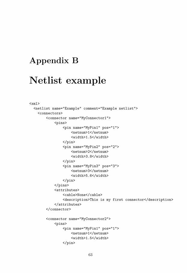
Appendix B
Netlist example
<xml><netlist name="Example" comment="Example netlist"><connectors>
<connector name="MyConnector1"><pins>
<pin name="MyPin1" pos="1"><netnum>1</netnum><width>1.5</width>
</pin><pin name="MyPin2" pos="2">
<netnum>2</netnum><width>3.8</width>
</pin><pin name="MyPin3" pos="3">
<netnum>3</netnum><width>5.6</width>
</pin></pins><attributes>
<cable>None</cable><description>This is my first connector</description>
</attributes></connector>
<connector name="MyConnector2"><pins>
<pin name="MyPin1" pos="1"><netnum>1</netnum><width>1.5</width>
</pin>
63

64 Chapter B. Netlist example
<pin name="MyPin2" pos="2"><netnum>2</netnum><width>3.8</width>
</pin><pin name="MyPin3" pos="3">
<netnum>3</netnum><width>5.6</width>
</pin></pins><attributes>
<cable>None</cable><description>This is my second connector</description>
</attributes></connector>
</connectors>
<nets><net name="MyNet1" num="1"></net><net name="MyNet2" num="2"></net><net name="MyNet3" num="3"></net>
</nets>
</netlist></xml>
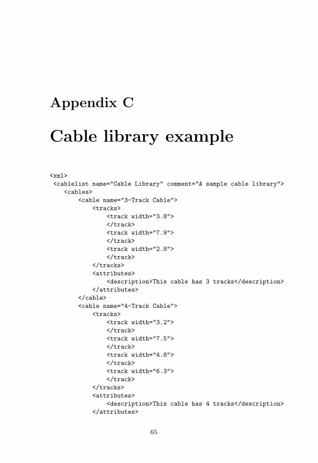
Appendix C
Cable library example
<xml><cablelist name="Cable Library" comment="A sample cable library">
<cables><cable name="3-Track Cable">
<tracks><track width="3.8"></track><track width="7.9"></track><track width="2.8"></track>
</tracks><attributes>
<description>This cable has 3 tracks</description></attributes>
</cable><cable name="4-Track Cable">
<tracks><track width="3.2"></track><track width="7.5"></track><track width="4.8"></track><track width="6.3"></track>
</tracks><attributes>
<description>This cable has 4 tracks</description></attributes>
65

</cable><cable name="5-Track Cable">
<tracks><track width="3.0"></track><track width="8.2"></track><track width="4.3"></track><track width="2.2"></track><track width="5.9"></track>
</tracks><attributes>
<description>This cable has 5 tracks</description></attributes>
</cable></cables>
</cablelist></xml>
Copyright
Svenska
Detta dokument halls tillgangligt pa Internet - eller dess framtida ersatt-are - under en langre tid fran publiceringsdatum under forutsattningatt inga extra-ordinara omstandigheter uppstar.
Tillgang till dokumentet innebar tillstand for var och en att lasa,ladda ner, skriva ut enstaka kopior for enskilt bruk och att anvanda detoforandrat for ickekommersiell forskning och for undervisning. Over-foring av upphovsratten vid en senare tidpunkt kan inte upphava dettatillstand. All annan anvandning av dokumentet kraver upphovsman-nens medgivande. For att garantera aktheten, sakerheten och tillgang-ligheten finns det losningar av teknisk och administrativ art.
Upphovsmannens ideella ratt innefattar ratt att bli namnd som up-phovsman i den omfattning som god sed kraver vid anvandning avdokumentet pa ovan beskrivna satt samt skydd mot att dokumentetandras eller presenteras i sadan form eller i sadant sammanhang somar krankande for upphovsmannens litterara eller konstnarliga anseendeeller egenart. For ytterligare information om Linkoping UniversityElectronic Press se forlagets hemsida http://www.ep.liu.se/
English
The publishers will keep this document online on the Internet - or itspossible replacement - for a considerable time from the date of publi-cation barring exceptional circumstances.
The online availability of the document implies a permanent per-mission for anyone to read, to download, to print out single copies foryour own use and to use it unchanged for any non-commercial researchand educational purpose. Subsequent transfers of copyright cannot re-voke this permission. All other uses of the document are conditionalon the consent of the copyright owner. The publisher has taken tech-nical and administrative measures to assure authenticity, security andaccessibility.
According to intellectual property law the author has the right to bementioned when his/her work is accessed as described above and to beprotected against infringement. For additional information about theLinkoping University Electronic Press and its procedures for publica-tion and for assurance of document integrity, please refer to its WWWhome page: http://www.ep.liu.se/
c© Tobias MarciszkoLinkoping, 18th May 2004
67