a tool for preliminary design of rockets - técnico lisboa · a tool for preliminary design of...

A Tool for Preliminary Design of Rockets

Diogo Marques Gaspar

Thesis to obtain the Master of Science Degree in

Aerospace Engineering

Supervisor : Professor Paulo Jorge Soares Gil

Examination Committee

Chairperson: Professor Fernando José Parracho LauSupervisor: Professor Paulo Jorge Soares GilMembers of the Committee: Professor João Manuel Gonçalves de Sousa Oliveira

July 2014

Dedicated to my Mother

iii

Acknowledgments

To my supervisor Professor Paulo Gil for the opportunity to work on this interesting subject and for all his

support and patience.

To my family, in particular to my parents and brothers for all the support and affection since ever.

To my friends: from IST for all the companionship in all this years and from Coimbra for the fellowship

since I remember.

To my teammates for all the victories and good moments.

v

Resumo

A unica forma que a humanidade ate agora conseguiu encontrar para explorar o espaco e atraves do

uso de rockets, vulgarmente conhecidos como foguetoes, responsaveis por transportar cargas da Terra

para o Espaco.

O principal objectivo no design de rockets e diminuir o peso na descolagem e maximizar o payload

ratio i.e. aumentar a capacidade de carga util ao seu alcance. A latitude e o local de lancamento,

a orbita desejada, as caracterısticas de propulsao e estruturais sao constrangimentos ao projecto do

foguetao.

As trajectorias dos foguetoes estao permanentemente a ser optimizadas, devido a necessidade de

aumento da carga util transportada e reducao do combustıvel consumido. E um processo utilizado nas

fases iniciais do design de uma missao, que afecta partes cruciais do planeamento, desde a concepcao

do veıculo ate aos seus objectivos globais.

O principal objectivo deste trabalho e encontrar o design mais adequado de um foguetao, para uma

orbita e carga especıficas, considerando a melhor trajectoria que pode ser utilizada. Foi desenvolvido

um programa que permite o estudo de diferentes configuracoes e a variacao dos parametros de design,

calculando para cada configuracao e conjunto de parametros as diferentes massas e dimensoes do

foguetao, para depois iterativamente com a trajectoria conseguir maximizar o payload ratio, minimizando

o peso na descolagem. Para validar o codigo foram feitas comparacoes com os resultados obtidos para

os lancadores Vega e Proton K/DM3. Por ultimo, e feita uma optimizacao do lancador Ariane 5 atraves

da variacao da sua configuracao e de parametros de design.

Palavras-chave: Multi-Estagios Rockets, Gravity Turn, Optimizacao de Trajectoria, Optimizacao

de Rockets, Maximizar o Payload Ratio.

vii

Abstract

The only way mankind can explore space is with the use of space launch vehicles, commonly known as

rockets, which carry payloads from Earth into Space.

The main goal in the rocket design is to reduce the gross lift-off weight (GLOW) and increase the

payload ratio, giving them the capacity of having the maximum amount of payload or its range. Launch

latitude, launch site, final kick-off location for payload, propulsion characteristics and, or, its own struc-

tural characteristics are all limitations in the launch vehicle’s design.

The trajectories of launch vehicles are permanently being optimized, due to the demand of increased

payload and reduced propellant requirements. Optimization of a trajectory is a process used in early

stages of the mission design, it affects crucial parts of mission planning, ranging from vehicle design to

even overall mission objectives.

The main objective of this study is to find the best design of a rocket for a specific orbit and payload

mass, considering the best trajectory that can be used. A tool was developed allowing the study of

different configurations and the variation of design parameters, calculating for each configuration and

parameters the different masses and dimensions that characterize a rocket, and then iteratively with the

trajectory will achieve the minimum GLOW and obtain the maximum payload ratio. In order to validate

the code comparisons with Vega and Proton K/DM3 launchers were made. At last an optimization of the

Ariane 5 launcher is made by varying its configuration and some design parameters.

Keywords: Multistage Rockets, Gravity Turn, Trajectory optimization, Rocket optimization, Max-

imize Payload Ratio.

ix

Contents

Acknowledgments . . . . . . . . . . . . . . . . . . . . . . . . . . . . . . . . . . . . . . . . . . . v

Resumo . . . . . . . . . . . . . . . . . . . . . . . . . . . . . . . . . . . . . . . . . . . . . . . . . vii

Abstract . . . . . . . . . . . . . . . . . . . . . . . . . . . . . . . . . . . . . . . . . . . . . . . . . ix

List of Tables . . . . . . . . . . . . . . . . . . . . . . . . . . . . . . . . . . . . . . . . . . . . . . xv

List of Figures . . . . . . . . . . . . . . . . . . . . . . . . . . . . . . . . . . . . . . . . . . . . . xviii

Nomenclature . . . . . . . . . . . . . . . . . . . . . . . . . . . . . . . . . . . . . . . . . . . . . . xx

Glossary . . . . . . . . . . . . . . . . . . . . . . . . . . . . . . . . . . . . . . . . . . . . . . . . xxi

1 Introduction 1

1.1 Goal of this work . . . . . . . . . . . . . . . . . . . . . . . . . . . . . . . . . . . . . . . . . 1

1.2 History of Rockets . . . . . . . . . . . . . . . . . . . . . . . . . . . . . . . . . . . . . . . . 1

1.3 Challenges in the design of a Rocket . . . . . . . . . . . . . . . . . . . . . . . . . . . . . . 3

1.4 Work overview . . . . . . . . . . . . . . . . . . . . . . . . . . . . . . . . . . . . . . . . . . 5

2 Rockets 7

2.1 Introduction to Rockets . . . . . . . . . . . . . . . . . . . . . . . . . . . . . . . . . . . . . . 7

2.2 Delta-V calculations . . . . . . . . . . . . . . . . . . . . . . . . . . . . . . . . . . . . . . . 7

2.3 Configuration . . . . . . . . . . . . . . . . . . . . . . . . . . . . . . . . . . . . . . . . . . . 8

2.3.1 Multi Stage . . . . . . . . . . . . . . . . . . . . . . . . . . . . . . . . . . . . . . . . 8

2.3.2 Boosters . . . . . . . . . . . . . . . . . . . . . . . . . . . . . . . . . . . . . . . . . 10

2.4 Structure . . . . . . . . . . . . . . . . . . . . . . . . . . . . . . . . . . . . . . . . . . . . . 11

2.4.1 Lower Stages . . . . . . . . . . . . . . . . . . . . . . . . . . . . . . . . . . . . . . . 11

2.4.2 Upper Stages . . . . . . . . . . . . . . . . . . . . . . . . . . . . . . . . . . . . . . . 11

2.4.3 Fairing . . . . . . . . . . . . . . . . . . . . . . . . . . . . . . . . . . . . . . . . . . . 12

2.4.4 Other components . . . . . . . . . . . . . . . . . . . . . . . . . . . . . . . . . . . . 13

2.5 Propulsion . . . . . . . . . . . . . . . . . . . . . . . . . . . . . . . . . . . . . . . . . . . . . 13

2.5.1 Solid Propellants . . . . . . . . . . . . . . . . . . . . . . . . . . . . . . . . . . . . . 14

2.5.2 Liquid Propellants . . . . . . . . . . . . . . . . . . . . . . . . . . . . . . . . . . . . 15

2.5.3 Hybrid Propellants . . . . . . . . . . . . . . . . . . . . . . . . . . . . . . . . . . . . 16

3 Ascent Rocket Trajectories 19

3.1 Trajectories . . . . . . . . . . . . . . . . . . . . . . . . . . . . . . . . . . . . . . . . . . . . 19

xi

3.1.1 Ascent Phase . . . . . . . . . . . . . . . . . . . . . . . . . . . . . . . . . . . . . . . 19

3.1.2 Gravity Turn . . . . . . . . . . . . . . . . . . . . . . . . . . . . . . . . . . . . . . . . 20

3.1.3 Free-flight phase . . . . . . . . . . . . . . . . . . . . . . . . . . . . . . . . . . . . . 21

3.1.4 Coast Phases . . . . . . . . . . . . . . . . . . . . . . . . . . . . . . . . . . . . . . . 24

3.1.5 Drag Model . . . . . . . . . . . . . . . . . . . . . . . . . . . . . . . . . . . . . . . . 25

3.1.6 Atmospheric Model . . . . . . . . . . . . . . . . . . . . . . . . . . . . . . . . . . . 26

3.1.7 Gravitational Model . . . . . . . . . . . . . . . . . . . . . . . . . . . . . . . . . . . 27

4 Rocket Knowledge Database 29

4.1 DB construction development . . . . . . . . . . . . . . . . . . . . . . . . . . . . . . . . . . 29

4.1.1 Small . . . . . . . . . . . . . . . . . . . . . . . . . . . . . . . . . . . . . . . . . . . 29

4.1.2 Medium . . . . . . . . . . . . . . . . . . . . . . . . . . . . . . . . . . . . . . . . . . 29

4.1.3 Heavy . . . . . . . . . . . . . . . . . . . . . . . . . . . . . . . . . . . . . . . . . . . 30

4.2 Information gathered . . . . . . . . . . . . . . . . . . . . . . . . . . . . . . . . . . . . . . . 30

4.3 Propellant Selection . . . . . . . . . . . . . . . . . . . . . . . . . . . . . . . . . . . . . . . 33

4.4 Mass Estimation Relationships . . . . . . . . . . . . . . . . . . . . . . . . . . . . . . . . . 34

5 Rocket Design Tool 37

5.1 Program Overview . . . . . . . . . . . . . . . . . . . . . . . . . . . . . . . . . . . . . . . . 37

5.2 Parametrization . . . . . . . . . . . . . . . . . . . . . . . . . . . . . . . . . . . . . . . . . . 38

5.3 Algorithm . . . . . . . . . . . . . . . . . . . . . . . . . . . . . . . . . . . . . . . . . . . . . 38

5.3.1 Mass Model . . . . . . . . . . . . . . . . . . . . . . . . . . . . . . . . . . . . . . . . 40

5.3.2 Trajectory . . . . . . . . . . . . . . . . . . . . . . . . . . . . . . . . . . . . . . . . . 42

6 Results 45

6.1 Validation . . . . . . . . . . . . . . . . . . . . . . . . . . . . . . . . . . . . . . . . . . . . . 45

6.1.1 Trajectory . . . . . . . . . . . . . . . . . . . . . . . . . . . . . . . . . . . . . . . . . 45

6.1.2 Mass model validation . . . . . . . . . . . . . . . . . . . . . . . . . . . . . . . . . . 47

6.2 Preliminary Design and Optimization . . . . . . . . . . . . . . . . . . . . . . . . . . . . . . 53

7 Conclusions 59

7.1 Future Work . . . . . . . . . . . . . . . . . . . . . . . . . . . . . . . . . . . . . . . . . . . . 61

Bibliography 67

A Nose Cone Geometries 69

A.1 Nose Cone Geometries . . . . . . . . . . . . . . . . . . . . . . . . . . . . . . . . . . . . . 69

A.1.1 Ogive . . . . . . . . . . . . . . . . . . . . . . . . . . . . . . . . . . . . . . . . . . . 69

A.1.2 Power . . . . . . . . . . . . . . . . . . . . . . . . . . . . . . . . . . . . . . . . . . . 70

A.1.3 Ellipse . . . . . . . . . . . . . . . . . . . . . . . . . . . . . . . . . . . . . . . . . . . 71

A.1.4 Haack . . . . . . . . . . . . . . . . . . . . . . . . . . . . . . . . . . . . . . . . . . . 71

xii

B Propellant properties 73

xiii

List of Tables

4.1 Characteristics gathered for each Stage of each Launcher . . . . . . . . . . . . . . . . . . 30

4.2 Structural factor for each Stage . . . . . . . . . . . . . . . . . . . . . . . . . . . . . . . . . 31

4.3 Thrust in Vacuum for each Stage . . . . . . . . . . . . . . . . . . . . . . . . . . . . . . . . 31

4.4 Length/Diameter ratio . . . . . . . . . . . . . . . . . . . . . . . . . . . . . . . . . . . . . . 31

4.5 Characteristics of Payload Fairings . . . . . . . . . . . . . . . . . . . . . . . . . . . . . . . 32

4.6 Ratio between Mass Fairing and GLOW . . . . . . . . . . . . . . . . . . . . . . . . . . . . 32

4.7 Propellant Specifications [1] . . . . . . . . . . . . . . . . . . . . . . . . . . . . . . . . . . . 33

5.1 Configuration and parameters introduced in the tool. . . . . . . . . . . . . . . . . . . . . . 38

5.2 Parameters of the Exterior Structure [2] [3]. . . . . . . . . . . . . . . . . . . . . . . . . . . 41

6.1 Vega Launcher - Main characteristics [4] . . . . . . . . . . . . . . . . . . . . . . . . . . . . 46

6.2 Proton K/DM3 - Main characteristics [5]. . . . . . . . . . . . . . . . . . . . . . . . . . . . . 46

6.3 Configuration and parameters introduced in the tool . . . . . . . . . . . . . . . . . . . . . 47

6.4 Mass Model Comparison - Vega . . . . . . . . . . . . . . . . . . . . . . . . . . . . . . . . 48

6.5 Volume Comparison - Vega . . . . . . . . . . . . . . . . . . . . . . . . . . . . . . . . . . . 48

6.6 Mass Model Comparison - PROTON K . . . . . . . . . . . . . . . . . . . . . . . . . . . . 50

6.7 Volume Comparison - Proton K . . . . . . . . . . . . . . . . . . . . . . . . . . . . . . . . . 51

6.8 Ariane 5 Launcher - Main characteristics. . . . . . . . . . . . . . . . . . . . . . . . . . . . 53

6.9 Parameters varied in the tool. . . . . . . . . . . . . . . . . . . . . . . . . . . . . . . . . . . 54

6.10 Optimal Configuration Achieved. . . . . . . . . . . . . . . . . . . . . . . . . . . . . . . . . 55

6.11 Mass Model Comparison - Ariane 5 . . . . . . . . . . . . . . . . . . . . . . . . . . . . . . 55

6.12 Volume Comparison - Ariane 5 . . . . . . . . . . . . . . . . . . . . . . . . . . . . . . . . . 56

B.1 Propellant Specifications . . . . . . . . . . . . . . . . . . . . . . . . . . . . . . . . . . . . . 73

xv

List of Figures

1.1 Space Shuttle . . . . . . . . . . . . . . . . . . . . . . . . . . . . . . . . . . . . . . . . . . . 3

2.1 Multistage Rocket configuration . . . . . . . . . . . . . . . . . . . . . . . . . . . . . . . . . 9

2.2 Parallel Staging configuration . . . . . . . . . . . . . . . . . . . . . . . . . . . . . . . . . . 11

2.3 Lower and Upper Stage VEGA . . . . . . . . . . . . . . . . . . . . . . . . . . . . . . . . . 12

2.4 Fairing - Vega . . . . . . . . . . . . . . . . . . . . . . . . . . . . . . . . . . . . . . . . . . 13

2.5 Interstage - Vega . . . . . . . . . . . . . . . . . . . . . . . . . . . . . . . . . . . . . . . . . 13

2.6 Sold Propellant Rocket Engine . . . . . . . . . . . . . . . . . . . . . . . . . . . . . . . . . 15

2.7 Liquid Propellant Rocket Engine . . . . . . . . . . . . . . . . . . . . . . . . . . . . . . . . 16

2.8 Hybrid Propellant Rocket Engine . . . . . . . . . . . . . . . . . . . . . . . . . . . . . . . . 17

3.1 Ascent Trajectory of the rocket . . . . . . . . . . . . . . . . . . . . . . . . . . . . . . . . . 20

3.2 Shooting Method for the free-flight phase . . . . . . . . . . . . . . . . . . . . . . . . . . . 25

3.3 Dynamic Pressure . . . . . . . . . . . . . . . . . . . . . . . . . . . . . . . . . . . . . . . . 26

3.4 Variation of Density - Standard Atmosphere . . . . . . . . . . . . . . . . . . . . . . . . . . 27

4.1 Max Payload vs Vol. Fairing . . . . . . . . . . . . . . . . . . . . . . . . . . . . . . . . . . . 32

5.1 Algorithm for the Design of the rocket . . . . . . . . . . . . . . . . . . . . . . . . . . . . . 40

5.2 Mass Model loop . . . . . . . . . . . . . . . . . . . . . . . . . . . . . . . . . . . . . . . . . 42

5.3 Trajectory . . . . . . . . . . . . . . . . . . . . . . . . . . . . . . . . . . . . . . . . . . . . . 43

6.1 Vega Launcher Simulation . . . . . . . . . . . . . . . . . . . . . . . . . . . . . . . . . . . . 49



6.4 Proton K Launch Simulation . . . . . . . . . . . . . . . . . . . . . . . . . . . . . . . . . . . 51



6.7 Ariane 5 Launch Simulation . . . . . . . . . . . . . . . . . . . . . . . . . . . . . . . . . . . 56



A.1 Ogive Nose Cone . . . . . . . . . . . . . . . . . . . . . . . . . . . . . . . . . . . . . . . . . 70

xvii

A.2 Power Nose Cone . . . . . . . . . . . . . . . . . . . . . . . . . . . . . . . . . . . . . . . . 70

A.3 Ellipse Nose Cone . . . . . . . . . . . . . . . . . . . . . . . . . . . . . . . . . . . . . . . . 71

A.4 Haack Nose Cone . . . . . . . . . . . . . . . . . . . . . . . . . . . . . . . . . . . . . . . . 72

xviii

Nomenclature

m Mass Flow Rate.

mfair Fairing Mass.

mfuel Fuel Mass.

mox Oxidizer Mass.

mo Rocket Section Mass.

∆V Delta-V.

TW Thrust to Weight Ratio.

CD Coefficient of drag.

Isp Specific Impulse.

mpay Payload Mass.

mp Propellant Mass.

ms Structural Mass.

Pamb Ambient pressure.

Pe Pressure at exit.

Vcirc Velocity - Circular Orbit.

Ve Exhaust velocity.

Vfuel Volume of fuel Tank.

Vox Volume of oxidizer Tank.

Vtank Volume of Tank.

Greek symbols

α Angle of attack.

γ Flight Path Angle.

xix

λ Payload Ratio.

Λ Mass Ratio.

µ gravitational parameter.

ρ Air Density.

ε Structural Ratio.

Roman symbols

bt Burning Time.

D Drag.

g gravitational acceleration.

g0 gravitational acceleration at sea level.

H Altitude.

p Pressure.

S Surface Area.

T Thrust.

th thickness.

X Downrange.

xx

Glossary

AP Ammonium Perchlorate

DB Double Base

ESA European Space Agency

F2 Liquid Fluorine

GEO Geosynchronous Earth Orbit

GLOW Gross Lift Off Weight

GTO Geostationary Transfer Orbit

GT Gravity Turn

H-2 Liquid Hydrogen

HMX Cyclo-tetramethylene tetranitramine

HTPB Hydroxyl-terminated polybutadiene

LEO Low Earth Orbit

LOX Liquid Oxygen

LVD Launch Vehicle Design

MDO Multi-Disciplinary Optimization

MER Mass Estimation Relationship

MMH Monomethylhydrazine

MR Mixture Ratio

OF Oxidizer to Fuel Ratio

RLV Reusable Launch Vehicle

RP-1 Refined Petroleum 1

TPBVP Two Point Boundary Value Problem

UDMH Unsymmetrical dimethylhydrazine

xxi

Chapter 1

Introduction

1.1 Goal of this work

The objective of this work is to develop a tool that will help design a multistage rocket, by obtaining

an preliminary sizing of the rocket and access the possible design trade-offs in order to maximize its

performance under some criteria.

1.2 History of Rockets

Modern rockets are the result of more than two thousand years of experiences, failures and inventions.

The first reported device to use rocket propulsion was developed in the 4th century b.C. in Greece, by

Archytas, who constructs and flies a small device, propelled by a jet of steam or compressed air. Later

on in the 13th century, during the war between China and Mongolia, the Chinese troops developed a

mixture of saltpeter, sulfur, and charcoal dust that produces colourful sparks and smoke, when ignited.

This powder was used to make fireworks, giving birth to the first concept of rocketry [6, 7].

In the beginning of the 17th century, Kasimierz Siemienowicz, commander of the Polish Royal Ar-

tillery, writes a manuscript on rocketry, Artis Magnae Artilleriae pars prima, which includes a design for

multistage rockets, essential technology for spaceflight rockets. Well-known scientists, Galileo Galilei

and Isaac Newton, 15th and 17th century respectively, develop the fundamental theories in the field

of physics, with their works in motion, particularly Newton’s Laws of Motion published in Philosophiae

Naturalis Principia Mathematica provides the foundation for all modern rocket science. Konstantin E.

Tsiolkovski known for his rocket equation, based on Newton’s second law of motion, and his work -

Research into Interplanetary Space by Means of Rocket Power, published in 1903, was an astronautics

pioneer, considered the father of cosmonautics and spaceflight. A few years later, in 1926, an American

college professor and scientist, Robert H. Goddard, known as the father of modern rocketry in the US,

builds and flies the world’s first liquid propellant rocket, essential to be able to reach space [6].

In the 1920s and 1930s, before World War II, scientists and amateur rocketeers attempted to use

rockets in every mean of transport, and though there were numerous failures, the experiments allowed

1

to improve rockets, making them more powerful and reliable. During World War II, the Germans built

and flew the most advanced rocket developed till then, the V2. The space era began in 1957 when the

Soviet Union amazed the world when it launched the world’s first artificial satellite, Sputnik 1. Less than

a month later, the Soviets followed with the launch of a satellite carrying a dog named Laika on board.

The great mind behind the V2 project was Dr. Wernher von Braun that led the development team that

launched Explorer 1 in 1958 by USA, and was also chief architect and engineer of the Saturn V Moon

Rocket. In 1961 Vostok 1 carried the first human into outer space cosmonaut Yuri Gagarin [8].

In the same year Freedom 7, launched by the US, makes a suborbital flight, because the rocket didn’t

have enough power to send the spacecraft to orbit. Until 1966 ten Gemini missions reached orbit, with

the help of a Titan missile. The Saturn V appears in the late sixties, capable of launching up to 118 tons

into Low Earth Orbit (LEO) and 41 tons to the Moon. After the end of Apollo program the investment

decreases, but new families of rockets appear. Delta family is one of the most versatile payload launch

rocket, with many configurations including multiple stages and heavy-lift-strap-on boosters that increase

payload capacity to high orbits [9].

In USSR several launchers have been designed and launched, the most relevant is Proton who

started is mission in 1965 and is still in active, recognized as a commercial workhorse of the Russian

space program. After launching the service module of the International Space Station in 2000, the four-

stage version of Proton launched numerous satellites for the Russian government and foreign customers

[6]. In 1975, European Space Agency (ESA) was created in Europe, rapidly starts with the development

of the Ariane family. ESA’s primary launcher is Ariane 5, in service since 1997, capable of delivering

between 6 to 10 tons into GTO and 21 tons into LEO.

In 1981 takes place the first flight of a Space Shuttle, by the US, carrying a crew and payloads, into

LEO, it’s presented in the figure 1.1. Russia tries to do the same by designing Buran, but it turns out

to be a disaster, because it only flies two times. Nowadays the essential to NASA’s plans is a new and

versatile space launch system, to replace the space shuttle. The constellation program that separates

human crews and payloads, for safety, is expected to combine the best of the past National Aeronautics

and Space Administration (NASA) decades of experience, with the best of present and future. Where

Ares I is a Crew Launch Vehicle, a two stage rocket with a crew capsule on top and Ares V will become

NASA’s primary heavy-lift cargo launch vehicle. ESA also developed Vega, for small payloads, capable

of placing multiple payloads into orbit. In cooperation with Russia, ESA allowed the launch of Soyuz-2

from French Guiana, capable of delivering 3 tons into GTO. Other countries, such as India, Japan and

China, although in a smaller scale, developed their own space programs. In China, Long March family

was the best know launcher, capable of delivering 12 tons into LEO. In Japan H-IIA was used to deliver 6

tons into GTO, and recently, H-IIB was developed, capable of delivering up to 8 tons into GTO. Launched

from an aircraft Pegasus is lifted to about 12 km and then, air launched from under the aircraft. This

special arrangement was developed to keep launch costs low for small orbital payloads [9].

2

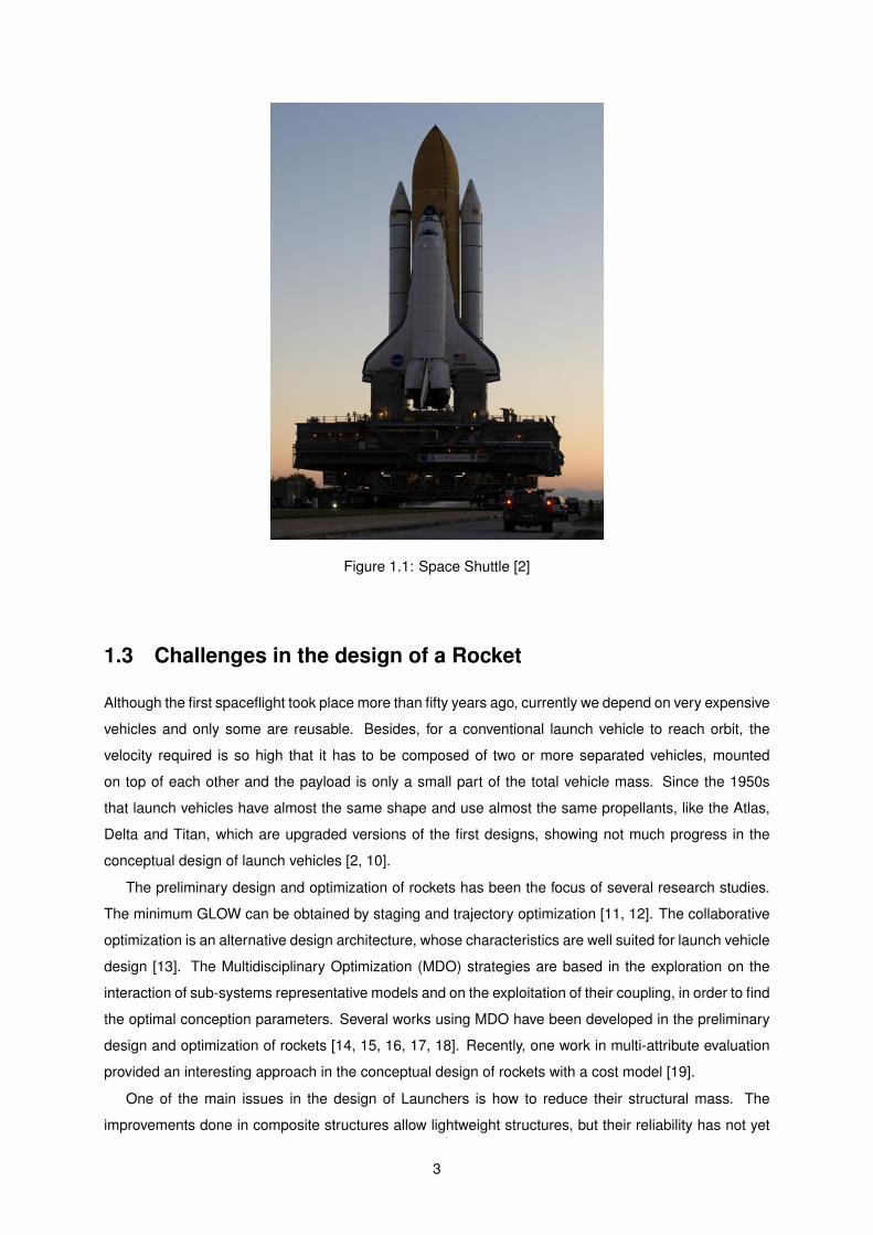
Figure 1.1: Space Shuttle [2]

1.3 Challenges in the design of a Rocket

Although the first spaceflight took place more than fifty years ago, currently we depend on very expensive

vehicles and only some are reusable. Besides, for a conventional launch vehicle to reach orbit, the

velocity required is so high that it has to be composed of two or more separated vehicles, mounted

on top of each other and the payload is only a small part of the total vehicle mass. Since the 1950s

that launch vehicles have almost the same shape and use almost the same propellants, like the Atlas,

Delta and Titan, which are upgraded versions of the first designs, showing not much progress in the

conceptual design of launch vehicles [2, 10].

The preliminary design and optimization of rockets has been the focus of several research studies.

The minimum GLOW can be obtained by staging and trajectory optimization [11, 12]. The collaborative

optimization is an alternative design architecture, whose characteristics are well suited for launch vehicle

design [13]. The Multidisciplinary Optimization (MDO) strategies are based in the exploration on the

interaction of sub-systems representative models and on the exploitation of their coupling, in order to find

the optimal conception parameters. Several works using MDO have been developed in the preliminary

design and optimization of rockets [14, 15, 16, 17, 18]. Recently, one work in multi-attribute evaluation

provided an interesting approach in the conceptual design of rockets with a cost model [19].

One of the main issues in the design of Launchers is how to reduce their structural mass. The

improvements done in composite structures allow lightweight structures, but their reliability has not yet

3

been proven. Liquid or hybrid propellants are used in upper stages, since they allow engine restart

and accurate orbit insertion [2]. Solid stages for boosters are usually cheaper to design, test, and

produce, compared to equivalent liquid or hybrid boosters, and don’t involve refrigeration requirements

[20]. Minimizing g-forces, for the comfort of the crew, allows better payload survivability and reduces the

structural loadings along the Launcher.

The calculation of the most adequate trajectory will increase the launchers efficiency. By minimizing

drag and gravity losses, a trade-off analysis needs to be performed [12, 21]. For the atmospheric flight,

several works consider the use of gravity turn (GT). [21, 22, 23]. For the exo-atmospheric flight there are

several methods for trajectory optimization used in works of the rocket design [24, 25, 22, 26].

It is often distinguished between two methods of numerical approaches in trajectory optimization,

they are direct and indirect methods. In a first overview the direct methods consist in discretizing the

state and the control and thus reduce the problem to a nonlinear optimization with constrains, and

indirect methods consist of solving numerically boundary value problem derived form the application

of the Pontryagin Maximum Principle and lead to the shooting methods. The paper of Betts gives a

overview of the most common and popular numerical methods for trajectory optimization problems.

However, it is difficult to reach with direct methods the precision provided by indirect methods [27].

The main advantages of using indirect methods are their high solution accuracy and the guarantee of

satisfying the optimal conditions of the solution [28, 29].

Increasing the number of stages allows saving mass and adapting thrust and engines to the altitude

where they will operate, but on the other hand, the design needs the minimum number of staging events,

to maximize the overall system reliability [10]. In order to increase the reliability, and decrease the cost of

transporting a payload into space, an extra effort is required during the initial design of the rocket and its

trajectory, allowing saving money and time. Higher reliability does not directly result from reuse, since the

necessary return capability, makes the launch vehicle more complex [30]. However, a noticeable cost

reduction can only be achieved with high reuse rates, which depend on very high reliability systems.

Due to the additional effort required to get the vehicle and/or stages back to Earth, reuse will be limited

to launches into LEO (300-600 kilometres level and 100 degrees orbit inclination), at least regarding

a near future. Ongoing missions (Geostationary Transfer Orbit (GTO)/ Geosynchronous Earth Orbit

(GEO), Moon, interplanetary) will therefore, continue to require expendable upper stages. Reusability is

considered to provide the major potential for future advancement of space transportation systems as it

saves production costs, however, the complexity of the vehicle and the mission, increase along with the

necessary return capability [2]. Typical objectives for reusable space launch systems are:

1. Cost reduction

2. Mission abort without loss of the launch vehicle

3. Return of payloads to the ground

4. Higher reliability

In analogy to aircraft, a fully reusable single-stage space transportation system, which delivers its

4

payload together with an expendable upper stage into LEO, is regarded as a goal. Various and some-

times very extensive US and European technology development and demonstration programs have

shown, however, that substantial technological progress is necessary before the target of a fully reusable

single-stage vehicle can be realized, particularly concerning: lightweight structures (tanks and high tem-

perature thermal protection system), propulsion system performance (rocket and air-breathing propul-

sion). In the foreseeable future, only multistage and partly reusable space transportation systems are

feasible [2, 31, 32, 33].

For future developments, a multitude of options are possible which lead to a variety of potential so-

lutions. However, options that substantially affect the most important parameters, affecting the design,

are limited: partial or full reusability (for a majority of missions expendable upper stages are necessary),

number of stages of launch and landing method (horizontal, vertical, with/without propulsion, winged),

propulsion (rocket, air-breathing propulsion, combinations) [24]. Based on experiences done with ex-

isting launch systems, extensive studies and technology activities, the following trends and limitations,

for future developments, can be foreseen: single-stage vehicles need new technologies, reuse of boost

stages leads to limited cost savings which do not justify the development and operating expenditure,

air-breathing propulsion is very complex and its integration into the overall design is demanding and

horizontal unpowered landing with wings is the feasible solution for the return of large rocket stages [34].

1.4 Work overview

Initially, rocket dynamics is presented, comprehending multistage rockets and learning the concepts of

different ratios, like structural, mass and payload. Not only simple staging is considered, parallel staging

is also taken into account and the propulsion technologies considered are solid, liquid and hybrid fuel,

contemplating their advantages and disadvantages.

In the field of rocket trajectories it is important to solve the problem considering the vertical ascent

phase and the gravity turn, because inside the atmosphere the ascent must be performed at zero lift

because even a slight build-up of normal forces can destroy the rocket. For the last part of trajectory

where the atmospheric forces are neglected an optimization method is used, a Two Point Boundary

Value Problem (TPBVP).

The creation of a database, that gathers information about current and past launchers, allows achiev-

ing realistic results, and functions as a heuristic, regarding the field of design. To accomplish this, a tool

is developed, in MATLAB, used, in a first stage, to design a rocket i.e. defining all the masses and dimen-

sions, taking into account specific constrains. After, it is used to optimize the last part of the trajectory

that fits such design, considering the Runge-Kutta integration during the ascent phase and gravity turn

and the free-flight phase, where was used a TPBVP using shooting as optimization method. The ∆V

losses are the key parameter for the convergence and achieve the final configuration. Two comparisons

with real cases will be made to validate the mass model and the trajectory, and then a set of simulations,

where the configuration and some parameters will be varied in order to optimize an existing Launcher.

5

Chapter 2

Rockets

In order to launch the satellites in orbit it’s necessary to escape from the Earth’s atmosphere and gravity.

To accomplish that, a large amount of ∆V is necessary and with the current technology only rockets

are able to achieve that. Currently, a SSTO is still impossible and only multistage configurations can

achieve space, that allow to optimize the structure and propulsion of each stage for different conditions.

Often, more than 90% of the rocket is propellant, meaning that rockets need a strong structure for

accommodate all the propellants and its powerful engines to burn them. Their structure is long and thin

allowing the reduction of drag during the trajectory. However this will bring structural problems when

normal loads are applied in the structure.

2.1 Introduction to Rockets

The Tsiolkovsky’s equation

V = Veln(m0

m

), (2.1)

where Ve is exhaust velocity, m0 the initial mass and m the mass of the rocket at each time. It allows the

determination of the velocity increase of a rocket propelled vehicle, regarding the propellant consumption

and the effective velocity of the exhaust gases. It is only valid for a constant exhaust velocity and in

absence of external forces, such as atmospheric drag and gravity.

2.2 Delta-V calculations

The ∆V budget of a mission is represented as

∆VDesign = ∆Vorbit + ∆Vgravity + ∆Vdrag, (2.2)

where ∆Vorbit is the injection velocity required for the desired orbit, ∆Vgravity and ∆Vdrag are respec-

tively the total gravity and drag losses. This equation allows us to make an estimate on the required ∆V

consumption and thus the required fuel needed to reach the trajectory and lower earth orbit.The Drag

7

and Gravity Losses are the most significant losses in ascent trajectory. Other losses due to the manoeu-

vring and static pressure difference at the nozzle exit during flights are considerably smaller compared

to gravity and drag losses. This ∆V budget must be larger or in exceptional cases equal to ∆V of the

mission, otherwise the payload/spacecraft wouldn’t be successful reaching the desired orbit.

The speed of a satellite in a circular orbit is defined by

Vorbit =

√µ

R, (2.3)

where R is the radius of the orbit and µ the gravitational parameter of the planet.

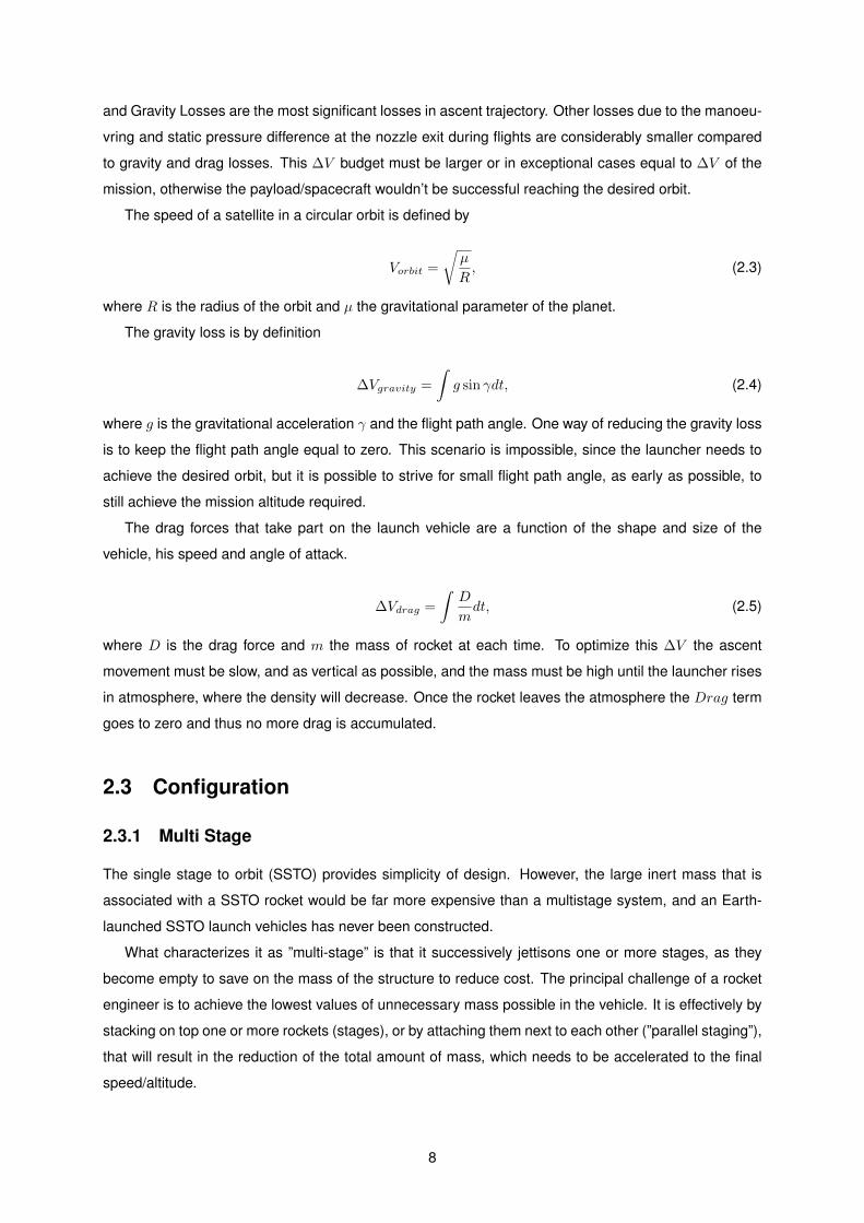
The gravity loss is by definition

∆Vgravity =

∫g sin γdt, (2.4)

where g is the gravitational acceleration γ and the flight path angle. One way of reducing the gravity loss

is to keep the flight path angle equal to zero. This scenario is impossible, since the launcher needs to

achieve the desired orbit, but it is possible to strive for small flight path angle, as early as possible, to

still achieve the mission altitude required.

The drag forces that take part on the launch vehicle are a function of the shape and size of the

vehicle, his speed and angle of attack.

∆Vdrag =

∫D

mdt, (2.5)

where D is the drag force and m the mass of rocket at each time. To optimize this ∆V the ascent

movement must be slow, and as vertical as possible, and the mass must be high until the launcher rises

in atmosphere, where the density will decrease. Once the rocket leaves the atmosphere the Drag term

goes to zero and thus no more drag is accumulated.

2.3 Configuration

2.3.1 Multi Stage

The single stage to orbit (SSTO) provides simplicity of design. However, the large inert mass that is

associated with a SSTO rocket would be far more expensive than a multistage system, and an Earth-

launched SSTO launch vehicles has never been constructed.

What characterizes it as ”multi-stage” is that it successively jettisons one or more stages, as they

become empty to save on the mass of the structure to reduce cost. The principal challenge of a rocket

engineer is to achieve the lowest values of unnecessary mass possible in the vehicle. It is effectively by

stacking on top one or more rockets (stages), or by attaching them next to each other (”parallel staging”),

that will result in the reduction of the total amount of mass, which needs to be accelerated to the final

speed/altitude.

8

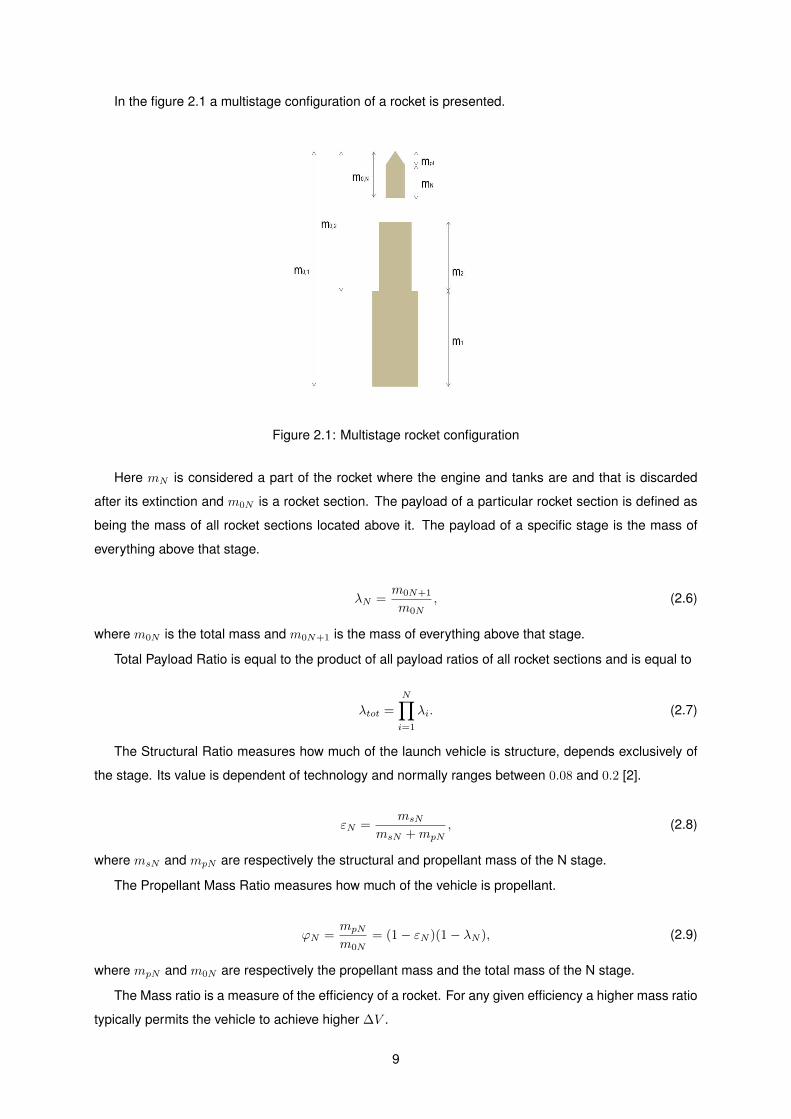
In the figure 2.1 a multistage configuration of a rocket is presented.

Figure 2.1: Multistage rocket configuration

Here mN is considered a part of the rocket where the engine and tanks are and that is discarded

after its extinction and m0N is a rocket section. The payload of a particular rocket section is defined as

being the mass of all rocket sections located above it. The payload of a specific stage is the mass of

everything above that stage.

λN =m0N+1

m0N, (2.6)

where m0N is the total mass and m0N+1 is the mass of everything above that stage.

Total Payload Ratio is equal to the product of all payload ratios of all rocket sections and is equal to

λtot =

N∏i=1

λi. (2.7)

The Structural Ratio measures how much of the launch vehicle is structure, depends exclusively of

the stage. Its value is dependent of technology and normally ranges between 0.08 and 0.2 [2].

εN =msN

msN +mpN, (2.8)

where msN and mpN are respectively the structural and propellant mass of the N stage.

The Propellant Mass Ratio measures how much of the vehicle is propellant.

ϕN =mpN

m0N= (1− εN )(1− λN ), (2.9)

where mpN and m0N are respectively the propellant mass and the total mass of the N stage.

The Mass ratio is a measure of the efficiency of a rocket. For any given efficiency a higher mass ratio

typically permits the vehicle to achieve higher ∆V .

9

ΛN =m0N

m0N −mpN=

1

1− ϕN, (2.10)

where the mpN and m0N are respectively the propellant mass and the total mass of the N stage and ϕ

is the propellant mass ratio.

The final burnout velocity is the sum of the burnout velocities of the individual stages, neglecting the

gravity and atmosphere.

V∗ =

N∏i=1

VeN ln(εN + (1− εN )λN ) (2.11)

The equations that described multistage rockets are almost equal as the single stage the term N

doesn’t exist [10].

2.3.2 Boosters

For larger payloads boosters stages are added to improve its performance, parallel staging in which two

stages are burning at the same time. These boosters are attached to the first stage of the launch vehicle

and their burn time is usually shorter than that of the first stage. Once they have burnt out they are

instantly ejected.

In this particular case, a ”zeroth” stage is defined as the combined booster rocket and first stage

while they burn together, and the fist stage as the remaining part of first stage after the boosters have

been discarded.

For ”zeroth” the structural and payload ratios are [10]:

ε0 =ms0 +ms1

ms0 +ms1 +mp0 +mp1, (2.12)

λ0 =m01 −mip1

m00, (2.13)

where ms0, mp0 are respectively the structural, propellant ratio of the ”zeroth” stage and mip1 is the

remaining propellant of the first stage when the ”zeroth” stage burnout.

The equations for the remaining of first stage are [10]:

ε1 =ms1

ms1 + (mp1 −mip1), (2.14)

λ1 =m02

m02 +ms1 + (mp1 −mip1), (2.15)

where m02 is the total mass of second stage and everything above.

10

Figure 2.2: Parallel staging configuration

2.4 Structure

Every kilogram that is transported to space requires fuel, regardless whether that kilogram is cargo,

crew, fuel, or part of the payload itself. The more the vehicle and the fuel weigh, fewer passengers and

smaller the payload the vehicle can carry.

A launch vehicle system can be divided into 3 main categories: Lower stages, Upper stages and

Fairing.

2.4.1 Lower Stages

Two basic functions take place in the lower stages. These are designed to both store the propellant

required to fulfil the mission, as well as provide the structural stability required by the entire vehicle, they

operate most of the time inside atmosphere. Usually, they are composed of a cylindrical section, which

is mainly filled with propellant: in average, 90% of the total mass is propellant. The liquid propellants

present in these vehicle stages, consist of fuel and oxidizer, which require the separation of each stage

in different tanks. For solid propellant, the rocket stage itself is filled with propellant, which presents a

typical grain section, with cylindrical or star form. The grain geometry defines the propellant mass flow

rate, and burning time. For heavy launchers usually the first stage has boosters attached, they increase

the payload mass that can be inserted in orbit.

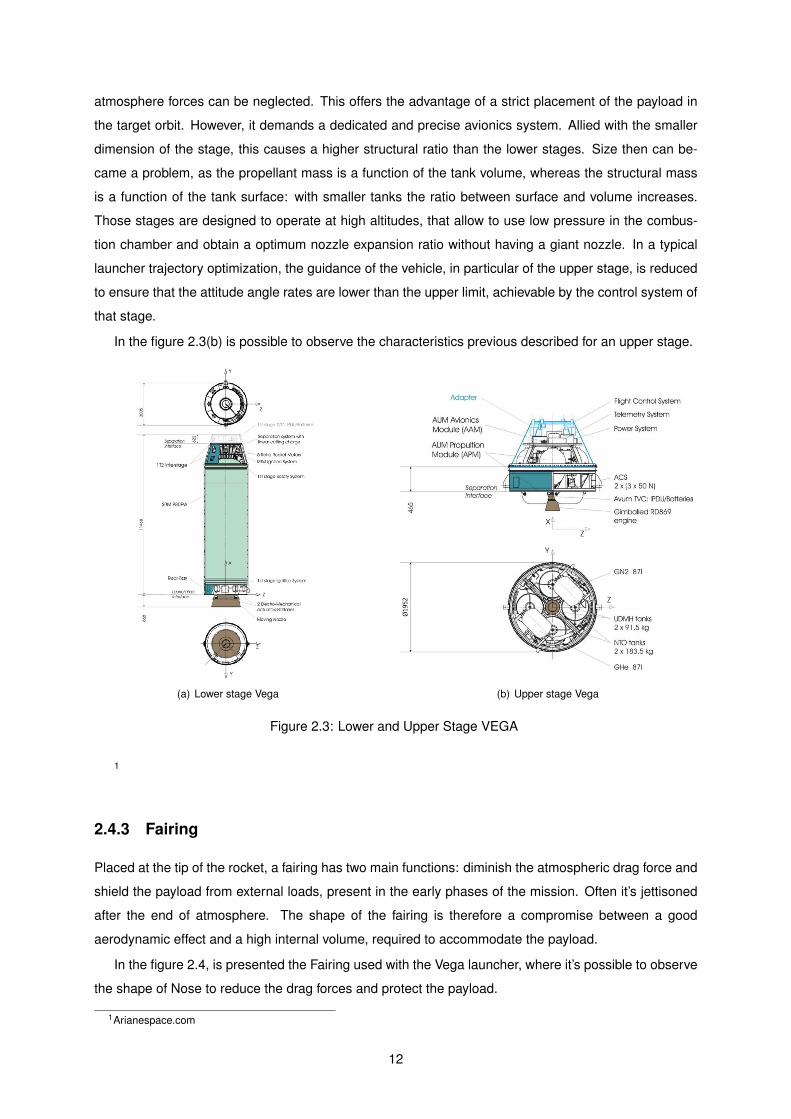
In the figure 2.3(a). is possible to observe the characteristics described for a lower stage of the Vega

rocket.

2.4.2 Upper Stages

The upper stage, usually the last stage, is active at higher altitudes, where the atmospheric effects are

not so important as in the beginning of the flight and the vehicle’s attitude can be improved because the

11

atmosphere forces can be neglected. This offers the advantage of a strict placement of the payload in

the target orbit. However, it demands a dedicated and precise avionics system. Allied with the smaller

dimension of the stage, this causes a higher structural ratio than the lower stages. Size then can be-

came a problem, as the propellant mass is a function of the tank volume, whereas the structural mass

is a function of the tank surface: with smaller tanks the ratio between surface and volume increases.

Those stages are designed to operate at high altitudes, that allow to use low pressure in the combus-

tion chamber and obtain a optimum nozzle expansion ratio without having a giant nozzle. In a typical

launcher trajectory optimization, the guidance of the vehicle, in particular of the upper stage, is reduced

to ensure that the attitude angle rates are lower than the upper limit, achievable by the control system of

that stage.

In the figure 2.3(b) is possible to observe the characteristics previous described for an upper stage.

(a) Lower stage Vega (b) Upper stage Vega

Figure 2.3: Lower and Upper Stage VEGA

1

2.4.3 Fairing

Placed at the tip of the rocket, a fairing has two main functions: diminish the atmospheric drag force and

shield the payload from external loads, present in the early phases of the mission. Often it’s jettisoned

after the end of atmosphere. The shape of the fairing is therefore a compromise between a good

aerodynamic effect and a high internal volume, required to accommodate the payload.

In the figure 2.4, is presented the Fairing used with the Vega launcher, where it’s possible to observe

the shape of Nose to reduce the drag forces and protect the payload.

1Arianespace.com

12

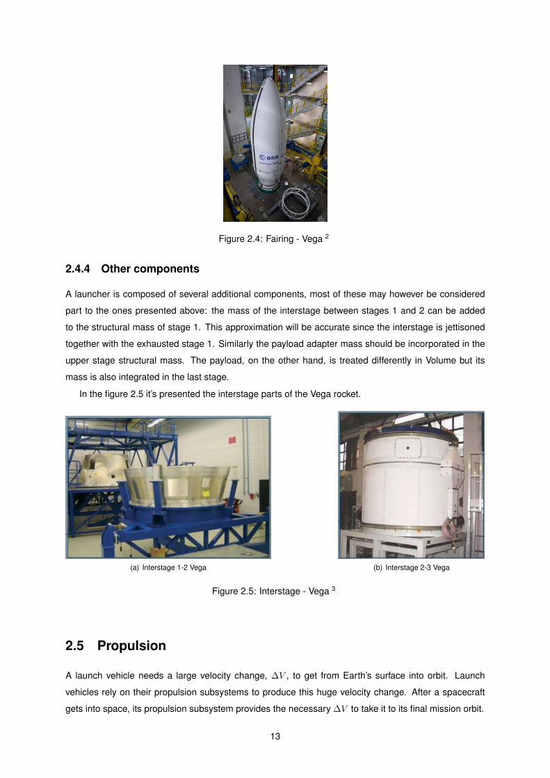
Figure 2.4: Fairing - Vega 2

2.4.4 Other components

A launcher is composed of several additional components, most of these may however be considered

part to the ones presented above: the mass of the interstage between stages 1 and 2 can be added

to the structural mass of stage 1. This approximation will be accurate since the interstage is jettisoned

together with the exhausted stage 1. Similarly the payload adapter mass should be incorporated in the

upper stage structural mass. The payload, on the other hand, is treated differently in Volume but its

mass is also integrated in the last stage.

In the figure 2.5 it’s presented the interstage parts of the Vega rocket.

(a) Interstage 1-2 Vega (b) Interstage 2-3 Vega

Figure 2.5: Interstage - Vega 3

2.5 Propulsion

A launch vehicle needs a large velocity change, ∆V , to get from Earth’s surface into orbit. Launch

vehicles rely on their propulsion subsystems to produce this huge velocity change. After a spacecraft

gets into space, its propulsion subsystem provides the necessary ∆V to take it to its final mission orbit.

13

The amount of thrust produced by the rocket depends on the mass flow rate through the engine and

the exit exhaust velocity.

T = mVe −Ae(Pe − Pamb) (2.16)

The main aspect regarding the nozzle is the altitude where it operates with maximum efficiency,

which defines the nozzle area exit Ae. The ratio of areas of nozzle throat and exit is the nozzle area

ratio. This means that for different stages or even during the same stages, the rocket will operate in

different scenarios, and equilibrium is required, between small ratio areas for low altitude operations,

and large ratio areas to allow the vacuuming along time. This is essential to achieve minimum mass and

physical dimensions. In this study, the thrust was selected by the user and assumed constant during

each stage, this result is a simplification, meaning the variation induced by the term Ae(Pe − Pamb) is

neglected [21, 35, 36, 11].

”Specific impulse” is the amount of momentum gained per weight of fuel consumed, the unit is sec-

onds, tells us the cost, in terms of the propellant mass, needed to produce a given thrust on a rocket.

The g0 is always the acceleration of gravity at the surface of the Earth. The great advantage is that the

exhaust velocity Ve may be obtained in English or Metric units.

Isp =Veg0

(2.17)

Different technologies have their own strengths and weaknesses, and their performance differ con-

siderably depending in which scenario are operating.

2.5.1 Solid Propellants

Solid propellant rockets have low specific impulse but relatively high storage density i.e. low volume,

making them good solutions for volume-limited applications, including missiles as well as first-stage

space boosters. Their Isp normally ranges between 175 seconds and 285 seconds. Like other chemical

rockets, they produce high thrust-to-weight ratios, and they are self-contained. Combustion of the pro-

pellant produces not only the energy but the working fluid for the rocket exhaust. There are no moving

parts or pumping requirements. Once ignited, the rocket motor performs without complication. Never-

theless, the very simplicity of the solid-propellant motor connotes lack of control. There is little room for

variation in the motor’s performance once the propellant grain is ignited, and thrust vectoring is difficult.

The solid rocket’s thrust is proportional to the surface area of the burning propellant, which in turn is

determined by the grain geometry. In all cases, the exterior shape of the grain is cylindrical, conical,

or spherical; however, the interior geometry can be designed to produce a range of thrust profiles (or

histories). The grain of an end burner is a solid cylinder, the burning surface has constant area as the

propellant is consumed; the thrust is constant, relatively low, and of long duration. If a cylindrical core

extends along the length of the motor, the initial surface is likely to be larger, hence, the thrust is larger

and the burn time is shorter. Furthermore, the burning area increases as propellant is consumed, so

14

thrust increases up to the point at which all of the propellant has been used. In a heavy lift launch ve-

hicle, solid propellant rockets are almost always built as a stand-alone system. In other words, they are

built as boosters, which are strap on, high thrust, independent systems [20].

In the figure 2.6, we can observe a simple representation of Solid Rocket Propellant,where oxidizer

and fuel are mixed together and cast into a solid mass called the grain and the hole down the middle

called the perforation.

Figure 2.6: Solid Propellant Rocket Engine [37]

2.5.2 Liquid Propellants

Liquid propellant rockets require more complexity for basic operation, but their superior performance and

precise controllability make them better suited for space applications. Their Isp normally ranges between

200 seconds and 500 seconds. Mixing oxidizer and fuel is a critical issue; the penalty for poor combus-

tion efficiency is severe, and the time during which the propellants must be combined is brief. Ignition

should be self-sustaining once thrusting has begun. Cooling of the rocket’s combustion chamber, throat,

and nozzle is a considerable problem because high performance means high temperatures, the internal

surfaces are exposed to high temperatures for long periods of time, and reliability and repeatability are

important if the motor is to be restarted or reused. The highest performance propellants are gaseous at

room temperature, and they must be cooled substantially for storage as liquids. This need for cryogenic

storage and pumping produces practical difficulties. Propellants must be loaded into the vehicle shortly

before launch, and there is an upper limit on the time that the propellants can be stored before they are

used or they boil away. Storage in space can be prolonged by keeping propellant tanks shaded from sun

light and by using tanks with high insulation, however, there are weight and volume limits on tank insula-

tion. The pressure in the combustion chamber is high, and propellants must be raised to an even higher

pressure to be injected into the motor. Pressurizing the fuel tanks and using high-pressure plumbing

throughout is a practical solution only for very small installations, as the required weight is high. Pres-

surized, non-combusting or catalytic monopropellants have been used for the attitude control of small

satellites. For large motors, a more practical approach is to use turbopumps to move the propellants,

with pumps powered either by the rocket motor itself or by auxiliary power generators. Rocket nozzles

for both solid- and liquid-propellant rockets must expand the flow efficiently. Early nozzles were simply

15

conical, as they were easy to build. However, most modern nozzles have a bell shape for more-efficient

isentropic expansion. As noted earlier, a fixed expansion ratio can be matched to ambient pressure at

just one altitude [20].

The mixture ratio of the propellant is normally specific to the engine and it represents the ratio be-

tween oxidizer and fuel. Usually it’s represented with oxidizer mass as numerator and fuel mass as

denominator.

MR =mox

mfuel(2.18)

The mass of oxidizer and fuel can be obtained by this two equations.

mox =(MR).mprop

(MR+ 1)(2.19)

mfuel =mprop

(MR+ 1)(2.20)

In the figure 2.7, we can see a simple representation of Liquid Propellant Rocket,where the oxidizer

and fuel are pumped into the combustion chamber.

Figure 2.7: Liquid Propellant Rocket Engine [37]

2.5.3 Hybrid Propellants

Hybrid rockets store the fuel as a solid and inject the oxidizer as a liquid or gas. Combustion occurs

along the grain surface, and it can be terminated by closing off the oxidizer flow. Their Isp normally

ranges between 260 and 400 sec. As might be expected, hybrid rockets have properties (good and

bad) of both solid-propellant and liquid-propellant rockets. The principal advantages are that they allow

energetic oxidizers (e.g., oxygen or hydrogen peroxide) to react with energetic fuels (e.g., hydrides of

magnesium, aluminium, or beryllium), they can be throttled, and they have high volumetric specific

impulse. Restarting and controlling thrust (magnitude and direction) are likely to be larger problems for

hybrids than for liquid-propellant rockets, the specific impulse is not quite as high, and the cryogenic

storage issue remains if liquid oxygen is used [20].

In the figure 2.8, we can see a simple representation of Hybrid Propellant Rocket,where the oxidizer

16

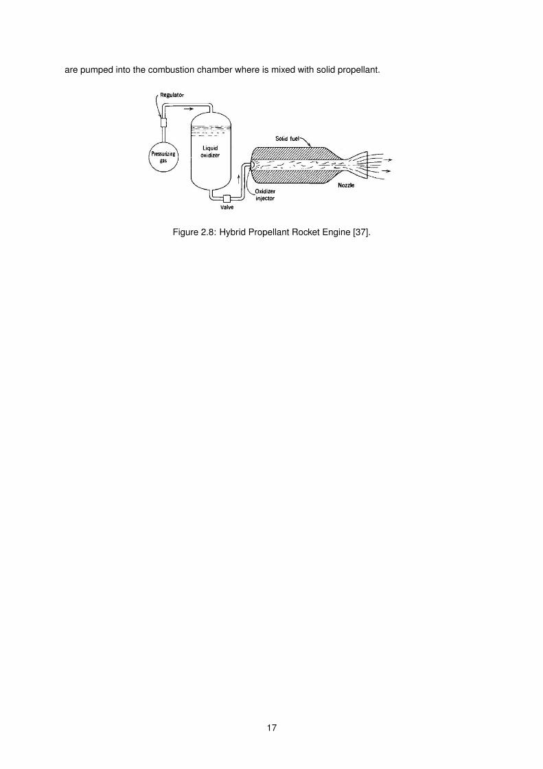
are pumped into the combustion chamber where is mixed with solid propellant.

Figure 2.8: Hybrid Propellant Rocket Engine [37].

17

Chapter 3

Ascent Rocket Trajectories

The rocket flight can be divided in two main phases: the atmospheric flight and the exo-atmospheric

flight. The frontier between them is not well defined, but can be linked to an altitude around 120 kilome-

tres, where atmosphere forces can be neglected.

3.1 Trajectories

In this section a description of the different flight phases is made comprehending the different phases of

the flight: the ascent phase, the gravity turn and the free-flight phase. Although the gravity turn guidance

is not optimal, it’s widely used in the trajectory of several works in rocket design. Only the last part in the

free-flight phase was optimized where was used a Two Point Boundary Value Problem (TPBVP).

Then the section provides an overview of all the different models that are used to simulate the condi-

tions that occur during the launch. Beginning with the drag model and then an overview of the environ-

ment which consists of an atmospheric model and the gravitational model.

3.1.1 Ascent Phase

A typical launcher starts its mission locked to the Launchpad. The engines are not yet ignited, or the

thrust provided is still lower than the vehicle weight. For solid propulsion, the time between ignition and

lift off is extremely short (less than 1 s). In the case of liquid propulsion, this time may be longer, allowing

the verification of the correct engine operations, before releasing the vehicle.

The first phase is a vertical lift off, required to gain velocity before the gravity turn phase and avoid

any contact with the launchpad tower. The duration of the ascent phase varies from vehicle to vehicle

and the current tendencies is to decrease it, because of the developments made in technology. The

necessary initial conditions include the flight path angle equal to 90 and velocity zero.

In the figure 3.1 is represented the launch sequence between lift-off and the final orbit, and the

division of altitude in two parts, one where the atmosphere can’t be neglected and other where the

atmosphere is neglected.

19

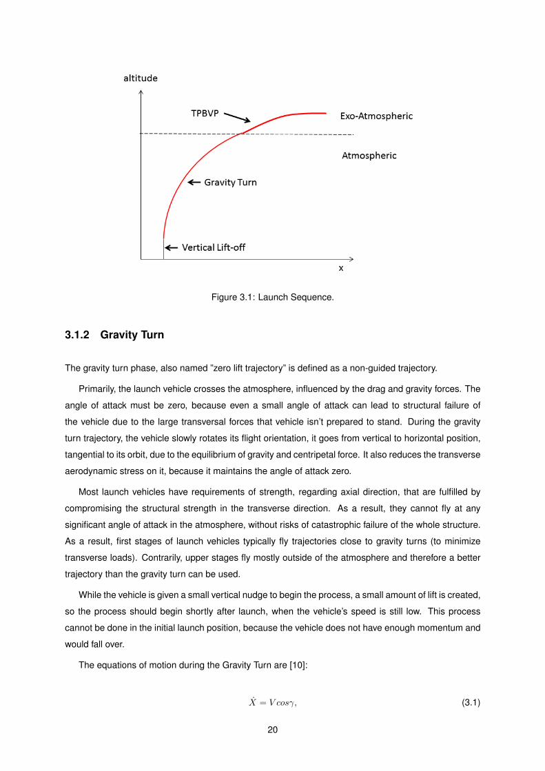
Figure 3.1: Launch Sequence.

3.1.2 Gravity Turn

The gravity turn phase, also named ”zero lift trajectory” is defined as a non-guided trajectory.

Primarily, the launch vehicle crosses the atmosphere, influenced by the drag and gravity forces. The

angle of attack must be zero, because even a small angle of attack can lead to structural failure of

the vehicle due to the large transversal forces that vehicle isn’t prepared to stand. During the gravity

turn trajectory, the vehicle slowly rotates its flight orientation, it goes from vertical to horizontal position,

tangential to its orbit, due to the equilibrium of gravity and centripetal force. It also reduces the transverse

aerodynamic stress on it, because it maintains the angle of attack zero.

Most launch vehicles have requirements of strength, regarding axial direction, that are fulfilled by

compromising the structural strength in the transverse direction. As a result, they cannot fly at any

significant angle of attack in the atmosphere, without risks of catastrophic failure of the whole structure.

As a result, first stages of launch vehicles typically fly trajectories close to gravity turns (to minimize

transverse loads). Contrarily, upper stages fly mostly outside of the atmosphere and therefore a better

trajectory than the gravity turn can be used.

While the vehicle is given a small vertical nudge to begin the process, a small amount of lift is created,

so the process should begin shortly after launch, when the vehicle’s speed is still low. This process

cannot be done in the initial launch position, because the vehicle does not have enough momentum and

would fall over.

The equations of motion during the Gravity Turn are [10]:

X = V cosγ, (3.1)

20

H = V sinγ, (3.2)

mV = T −D − (mg − mV 2

Re+H)sin(γ), (3.3)

γ = − 1

V(g − V 2

Re+H)cos(γ), (3.4)

where the X and H are respectively the downrange distance and altitude of the rocket, the V and γ are

respectively the velocity and flight path angle of the rocket, the T and D are respectively the thrust and

drag, the Re and m are respectively the radius of the Earth and the mass of rocket at each moment and

g the local gravity.

The trajectory data includes altitude, flight path angle variation, thrust, drag and total system mass.

In order to integrate the equations of movement a MATLAB standard solver for ordinary differential

equations, commonly named ODEs, was used the function ode45. This function implements a Runge-

Kutta method with a variable time step.

3.1.3 Free-flight phase

As the vehicle emerges from the atmosphere a better trajectory than the gravity turn can be used. It has

a (present) position and velocity, and it is desired to achieve a different position and velocity at thrust

termination. The only two forces that can cause the vehicle to accomplish the desired position and

velocity changes are thrust and gravity.

Continuous problems of trajectory optimization are traditionally solved by direct or indirect methods

[27]. We want to minimize the final time i.e. the duration of this phase, less time means less propellant

because we assumed a constant thrust, this is therefore equivalent to minimize the GLOW. In boundary

value problems, finding a good initial guess is a major difficulty. There is no formula, the engineer or the

user must have some insight into the problem through numerical experimentation.

The TPBVP, only starts after the Knudsen number condition, that tell us that we are in exo-atmospheric

conditions. Here the drag forces are neglected. This problem was solved numerically by a shooting

method, based on the application of the Pontryagin Maximum Principle. The shooting method is known

to be hard to initialize, and the convergence is difficult to obtain because of discontinuities of the optimal

control [38].

For minimum time problems [28], the cost function can be written as

J = tf , (3.5)

subject to 4 state equations

x = Vx (3.6)

21

y = Vy (3.7)

Vx =T

m0 − mtcos(θ) (3.8)

Vy =T

m0 − mtsin(θ)− g (3.9)

the initial conditions of TPBVP are the final conditions of gravity turn.

t0 = t (3.10)

x0 = x (3.11)

y0 = y (3.12)

Vx0 = Vx (3.13)

Vy0 = Vy (3.14)

the final conditions, for the particular case of circular orbit are

yf = Re + h (3.15)

Vxf = V c (3.16)

Vyf = 0 (3.17)

condensed as

Ψ =

Ψ1

Ψ2

Ψ3

=

yf − (Re + h)

Vxf − VcVyf

= 0 (3.18)

We know that tf and xf are free variables. The Hamiltonian is

H = λ1X + λ2Y + λ3Vx + λ4Vy (3.19)

The Euler-Lagrange Equations λ = −Hx, Hu = 0, so the costate equations are.

λ1 = −dHdx

= 0 (3.20)

λ2 = −dHdy

= 0 (3.21)

Thus

λ1 = c1 (3.22)

λ2 = c2 (3.23)

22

λ3 = − dHdvx

= −λ1 (3.24)

λ4 = −dHdvy

= −λ2 (3.25)

Since the λ1 and λ2, are constant

λ3 = −c1t− c3 (3.26)

λ4 = −c2t+ c4 (3.27)

The control equation is found from

dH

dθ= −λ3

T

msin(θ + λ4

T

mcos(θ) = 0 (3.28)

Thus, we have, a bi-linear tangent law.

tan(θ) =λ4λ3

=−c2t+ c4−c1t+ c3

(3.29)

and then

cos(θ) = (±λ3√λ23 + λ24

) (3.30)

sin(θ) = (±λ4√λ23 + λ24

) (3.31)

Applying transversality condition and the Minimum Principle, which states that the Hamiltonian must

be minimized [28]. We have a λ1 = c1 and λ1f = c0, so c1 = 0. Therefore we obtain the linear tangent

steering law.

tan(θ) =c2t

−c3+−c4−c3

= at+ b, (3.32)

this law is used in guidance systems, with updates for a and b at each second.

At this point, we have a well defined TPBVP, with four state equations, and four costate equations.

x = Vx (3.33)

y = Vy (3.34)

Vx =F

m0 − mt(−λ3√λ23 + λ24

) (3.35)

Vy =F

m0 − mt(−λ4√λ23 + λ24

)− g (3.36)

λ1 = 0 (3.37)

λ2 = 0 (3.38)

λ3 = −λ1 (3.39)

23

λ4 = −λ2 (3.40)

Thus there are eight differential equations.

x = f(t, x, λ) (3.41)

λ = g(t, x, λ) (3.42)

Now there are five initial conditions and five final conditions.

The steps that shooting method uses are the following:

1. Guess λ10, λ20, λ30, λ40 and tf

2. Integrate the x and λ forward to t = tf

3. Compute the final conditions:

Ψ1 = yf − hcirc +REarth (3.43)

Ψ2 = Vxf − Vcirc (3.44)

Ψ3 = Vyf (3.45)

Ψ4 = λ1f (3.46)

Ψ5 = Hf + 1 (3.47)

where λ and tf are changed iteratively

4. Until the convergence on Ψi(λ0,tf ) = 0 for i = 1, .., 5

In the figure 3.2, it’s possible to observe, the initial conditions, and a few iterations of Shooting Method

until the convergence has achieved.

To solve this last part of the trajectory a Matlab function has been used. The bvp4c solves boundary

value problems for ordinary differential equations. For many optimal control problems, as in our case,

is the best option. However, we must pay attention to the limitations of bvp4c, more specifically a good

initial guess is important to get an accurate solution, if a solution exists. By applying the minimum

principle, we can convert the problem into a BVP and solve it with indirect methods. Nevertheless, for

problems with constraints, does not necessarily hold although the Hamiltonian still achieves the minimum

within the admissible control set [28].

3.1.4 Coast Phases

The coast phases are performed between the jettison of a stage and the ignition of the next one. So

the propagation of the trajectory is only influenced by the gravitational force, in real cases aerodynamic

24

Figure 3.2: Shooting Method for the free-flight phase

forces need to be considered, but in this case as we know there is no angle of attack during atmospheric

flight so they can be disregarded. The coast phases are often used for injection into GTO and for

interplanetary trajectories, where the constant thrust can’t be applied.

3.1.5 Drag Model

The drag coefficient is a function of the atmospheric conditions (local flow Mach number) and the geom-

etry of the rocket. Obtaining information of aerodynamic data launchers is almost impossible, because

this data is kept secret. To be more precise a Computational Fluid Dynamics (CFD) analysis is needed

to get results closer to reality. An approach for analytical formulas for each Nose Cone was tried, but

lack of available information didn’t allow to go further in that analysis [39]. An assumption was made,

the drag force is independent of the length of the vehicle (assuming skin friction drag to be negligible).

D =1

2ρCDSrefV

2, (3.48)

where ρ is the density of the atmosphere, the Cd is the drag coefficient, Sref is the cross-sectional area

of the body and V is the velocity of the vehicle.

A simple model for the Cd was adopted [40]. An interpolation of the values for the first stage from

table 4.16 in page 269 was made. The Cd only varies with the Mach Number. The resulting equation is

Cd = −3E−6M6 + 0.0002M5 − 0.0046M4 + 0.053M3 − 0.2806M2 + 0.6211M + 0.0568 (3.49)

This equation have a regression of 90% with a polynomial fit of 6th order.

25

The program shows the dynamic pressure during atmospheric phase

q =1

2ρV 2, (3.50)

where ρ is the air density and V the velocity of the rocket.

The dynamic pressure has two important properties. The quadratic dependence on velocity means

that the lift and drag increase very rapidly as the rocket accelerates. The effect of drag on first-stage

acceleration is significant, the acceleration of the vehicle is often almost constant even though the mass

is reducing. The dynamic pressure also depends on the atmospheric density, which decreases rapidly as

the rocket gains altitude. Thus, with velocity increasing, and density decreasing, with time after launch,

every launcher passes through a condition known as maximum dynamic pressure that happens around

an altitude of about 10 kilometres. This is the time when the atmospheric forces are at their maximum,

and when the risk to the structural integrity of the rocket is greatest. To reduce the risk, if the vehicle’s

structure isn’t designed to support the loads it experiences, the engines are throttled down in order to

reduce the forces acting on the vehicle. The figure 3.3 shows how the Dynamic pressure varies with

altitude.

Figure 3.3: Dynamic Pressure

3.1.6 Atmospheric Model

The earth atmosphere is a thin layer around the planet and during the flight to orbit the performance of

the launch vehicle will be influenced by its environment.

Therefore, it is important to understand and model the atmosphere’s properties (temperature, pres-

sure and density) with accurate approximations. Many atmospheric models have already been devel-

oped to answer the needs of the design of launch vehicles and the analysis of their trajectory.

26

In 1962 and 1976, two U.S conventions of Standard Atmosphere were developed, the first regarding

velocities for altitudes higher than 86 kilometres, and the second one regarding velocities for altitudes

lower than 86 kilometres [41].

In this work, the U.S. Standard Atmosphere Convention of 1976 was used as a reference, for altitudes

lower than 86 kilometres, and the 1962 U.S. Standard Atmosphere was followed for altitudes above 86

kilometres, it models atmosphere up to 2000 kilometres. The last layer ranges between 700 and 2000

kilometres [35].

The Knudsen number will define the boundary between the atmospheric and exo-Atmospheric flight,

i.e. it will define the end of gravity turn and the beginning of the third part of flight. The Knudsen number

is dimensionless defined as

Kn =λknL

(3.51)

In equation 3.51, λkn is the mean free path of free-stream molecules and L is a length characteristic,

the value assumed was the cone radius that it’s the same of last stage radius. The different flow regimes

are classified as shown below:

ContinuumFlow Kn < 0.01 (3.52)

TransitionF low 0.01 < Kn < 10 (3.53)

Free−MolecularF low Kn > 10 (3.54)

The next figure 3.4 represents the variation of Density along the first 120 kilometres of the Atmo-

sphere, where the effects of Drag can’t be neglected.

Figure 3.4: Atmospheric Density

3.1.7 Gravitational Model

The external force caused by gravity is the main force that acts on the launch vehicle. Gravity is the

natural phenomenon by which physical bodies are attracted to each other with a force proportional to

27

their masses. This work assumed a flat and non-rotating Earth so that g0 is constant and terms involving

its angular velocity are ignored [21].

The local gravity is calculated with the following equation

g =g0

1 + hRe

, (3.55)

where h is the current altitude, Re = 6378 kilometres the radius of Earth and g0 = 9.81(m/s) surface

gravity.

28

Chapter 4

Rocket Knowledge Database

For a better understanding of the differences between launchers, and to compare converging parameters

between them, a database of well-known launchers was developed. It gathers information about their

different masses, dimensions and propulsion, to understand if the concept of new designed rockets is

”real”, and if their values can be compared with similar launchers. The database can also be used as a

starting point or to help define bounds of parameters.

4.1 DB construction development

Although there is information available about more than a hundred launch rockets, only four to five were

considered, for each class. The database was developed and divided by ”how much payload they can

deliver in specific orbit?”. Regarding this criteria three different classes of launchers were defined.

4.1.1 Small

Small launchers are mainly used for transferring payloads into Low Earth Orbit (LEO), they can deliver

up to 2 tons at LEO [2]. Information about four launchers of this class was gathered, they are Rockot

[42], Pegasus-XL [43], Falcon 1 [44] and Vega [4]. None of them have boosters in their configuration.

4.1.2 Medium

Medium launchers serve to place satellites into all Earth orbits: LEO, including polar orbits, medium

Earth orbits (MEOs), GTOs, GEO and Earth escape missions. They can deliver between 2 and 15 tons

at LEO and 3 to 6 tons at GEO [2]. These kind of launchers feature the possibility of having boosters.

Information about 5 launchers was gathered, they are Soyuz [45], CZ-4B, Zenit-SL [46], H-IIA and Delta

IV-M [47].

29

4.1.3 Heavy

Heavy-lift launch vehicles (HLLVs) mainly launch communications satellites into GTOs and are used

specifically for launching very heavy payloads. They can deliver more than 15 tons at LEO and 6 tons

at GEO [2]. Except some launchers, they all have boosters. They have long burning times of first-stage,

i.e. they spend more time leaving the Earth atmosphere, compared to Small and Medium launchers.

Information about 4 launchers was gathered, they are Ariane 5 [48], Proton K-DM3 [5], Atlas V [49] and

STS known as Space Shuttle [3].

4.2 Information gathered

For each stage of each launcher a lot of information was available in the Users Manual but only the

principal characteristics that define a rocket were selected. In the table 4.1 are a list of the information

gathered for the selected launchers.

Characteristics UnitsClass Small/Medium/HeavyYear -

Engine -Length m

Diameter mLength/Diameter -

Take-off mass kgPropellant mass kgStructural mass kgStructural factor kg

Propellants -Burning duration s

Thrust (vac) kNIsp (vac) s

T/W -Remarks -

Table 4.1: Characteristics gathered for each Stage of each Launcher

Some information wasn’t available for all launchers, for example the Nozzle Area Ratio is one charac-

teristic that is very difficult to obtain, such as Aerodynamic Performance. The most important information

gathered is about structural factor of each stage, that allows us to know how much mass of each stage

is structure, and to give an appropriate range of values of Structural factor of each stage for Mass model

developed in this work. The medium value obtained was used in mass model as first value for the

iterations of Structural factor. The range of values is presented in the table 4.2.

30

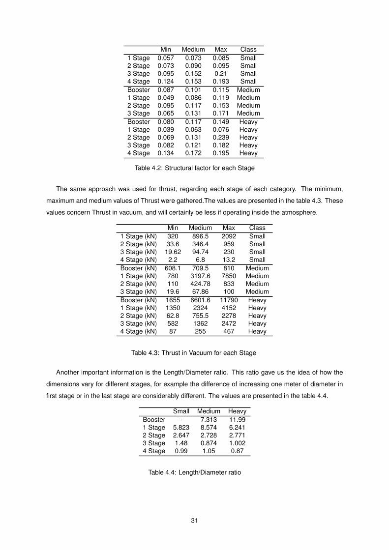
Min Medium Max Class1 Stage 0.057 0.073 0.085 Small2 Stage 0.073 0.090 0.095 Small3 Stage 0.095 0.152 0.21 Small4 Stage 0.124 0.153 0.193 SmallBooster 0.087 0.101 0.115 Medium1 Stage 0.049 0.086 0.119 Medium2 Stage 0.095 0.117 0.153 Medium3 Stage 0.065 0.131 0.171 MediumBooster 0.080 0.117 0.149 Heavy1 Stage 0.039 0.063 0.076 Heavy2 Stage 0.069 0.131 0.239 Heavy3 Stage 0.082 0.121 0.182 Heavy4 Stage 0.134 0.172 0.195 Heavy

Table 4.2: Structural factor for each Stage

The same approach was used for thrust, regarding each stage of each category. The minimum,

maximum and medium values of Thrust were gathered.The values are presented in the table 4.3. These

values concern Thrust in vacuum, and will certainly be less if operating inside the atmosphere.

Min Medium Max Class1 Stage (kN) 320 896.5 2092 Small2 Stage (kN) 33.6 346.4 959 Small3 Stage (kN) 19.62 94.74 230 Small4 Stage (kN) 2.2 6.8 13.2 SmallBooster (kN) 608.1 709.5 810 Medium1 Stage (kN) 780 3197.6 7850 Medium2 Stage (kN) 110 424.78 833 Medium3 Stage (kN) 19.6 67.86 100 MediumBooster (kN) 1655 6601.6 11790 Heavy1 Stage (kN) 1350 2324 4152 Heavy2 Stage (kN) 62.8 755.5 2278 Heavy3 Stage (kN) 582 1362 2472 Heavy4 Stage (kN) 87 255 467 Heavy

Table 4.3: Thrust in Vacuum for each Stage

Another important information is the Length/Diameter ratio. This ratio gave us the idea of how the

dimensions vary for different stages, for example the difference of increasing one meter of diameter in

first stage or in the last stage are considerably different. The values are presented in the table 4.4.

Small Medium HeavyBooster - 7.313 11.991 Stage 5.823 8.574 6.2412 Stage 2.647 2.728 2.7713 Stage 1.48 0.874 1.0024 Stage 0.99 1.05 0.87

Table 4.4: Length/Diameter ratio

31

Also, the principal characteristics about payload fairing, which were also gathered for each launcher,

are listed in the table 4.5.

Characteristics UnitsVolume m3

Mass kgLength m

Diameter mLength/Diameter -

Payload kg

Table 4.5: Characteristics of Payload Fairings

With the information gathered about the Payload, an estimate of how much of GLOW is from Fairing.

This information provides us a good estimate for the mass of the Fairing and its presented in the table

4.6.

Small Medium Heavy% Massfairing/GLOW 0.92 0.96 0.9

Table 4.6: Ratio between Mass Fairing and GLOW

The GLOW is already defined and the mass of Fairing is estimated by a heuristic relation. A relation-

ship between the mass and the volume of the Fairing was developed, for each class of launchers. An

exponential regression was used for the following equations:

Figure 4.1: Max Payload vs Volume Fairing

For the class of Small Launchers, the Volume is defined by

Vfairing = 0.6959e0.0044Mfairing (4.1)

For the class of Medium Launchers, the Volume is defined by


32

For the class of Heavy Launchers, the Volume is defined by


The Fairing is included in the last stage. So the diameter of the base of Nose Cone will be equal to

the diameter of the last stage. Knowing the Volume, and the type of Nose Cone (more in Appendix A),

there is enough information to design the Fairing from the initial design point of view. The length of the

Nose Cone is added to the rest of the launcher to calculate the total dimensions of the Launcher.

The volume of an Elliptical cone is defined by

VEllipticalCone =πd2h

6, (4.4)

with this formula, knowing the Volume and the diameter (d), all the dimensions are obtained and the

Nose Cone can be included in the calculations.

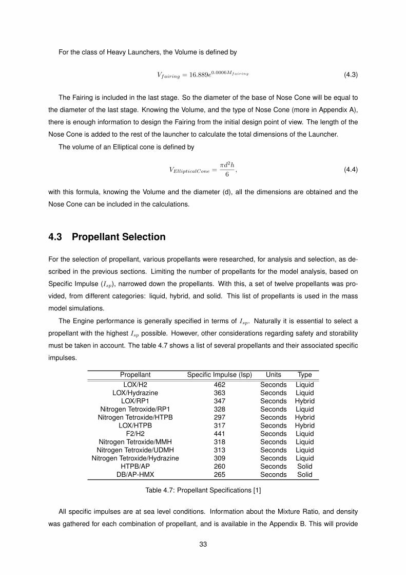
4.3 Propellant Selection

For the selection of propellant, various propellants were researched, for analysis and selection, as de-

scribed in the previous sections. Limiting the number of propellants for the model analysis, based on

Specific Impulse (Isp), narrowed down the propellants. With this, a set of twelve propellants was pro-

vided, from different categories: liquid, hybrid, and solid. This list of propellants is used in the mass

model simulations.

The Engine performance is generally specified in terms of Isp. Naturally it is essential to select a

propellant with the highest Isp possible. However, other considerations regarding safety and storability

must be taken in account. The table 4.7 shows a list of several propellants and their associated specific

impulses.

Propellant Specific Impulse (Isp) Units TypeLOX/H2 462 Seconds Liquid

LOX/Hydrazine 363 Seconds LiquidLOX/RP1 347 Seconds Hybrid

Nitrogen Tetroxide/RP1 328 Seconds LiquidNitrogen Tetroxide/HTPB 297 Seconds Hybrid

LOX/HTPB 317 Seconds HybridF2/H2 441 Seconds Liquid

Nitrogen Tetroxide/MMH 318 Seconds LiquidNitrogen Tetroxide/UDMH 313 Seconds Liquid

Nitrogen Tetroxide/Hydrazine 309 Seconds LiquidHTPB/AP 260 Seconds Solid

DB/AP-HMX 265 Seconds Solid

Table 4.7: Propellant Specifications [1]

All specific impulses are at sea level conditions. Information about the Mixture Ratio, and density

was gathered for each combination of propellant, and is available in the Appendix B. This will provide

33

more realistic results for the results of the mass model.

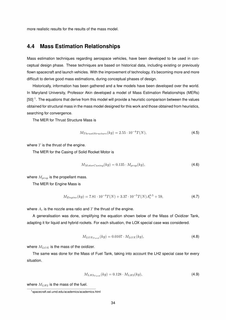
4.4 Mass Estimation Relationships

Mass estimation techniques regarding aerospace vehicles, have been developed to be used in con-

ceptual design phase. These techniques are based on historical data, including existing or previously

flown spacecraft and launch vehicles. With the improvement of technology, it’s becoming more and more

difficult to derive good mass estimations, during conceptual phases of design.

Historically, information has been gathered and a few models have been developed over the world.

In Maryland University, Professor Akin developed a model of Mass Estimation Relationships (MERs)

[50] 1. The equations that derive from this model will provide a heuristic comparison between the values

obtained for structural mass in the mass model designed for this work and those obtained from heuristics,

searching for convergence.

The MER for Thrust Structure Mass is

MThrustStructure(kg) = 2.55 · 10−4T (N), (4.5)

where T is the thrust of the engine.

The MER for the Casing of Solid Rocket Motor is

MMotorCasing(kg) = 0.135 ·Mprop(kg), (4.6)

where Mprop is the propellant mass.

The MER for Engine Mass is

MEngine(kg) = 7.81 · 10−4T (N) + 3.37 · 10−5T (N)A0.5r + 59, (4.7)

where Ar is the nozzle area ratio and T the thrust of the engine.

A generalisation was done, simplifying the equation shown below of the Mass of Oxidizer Tank,

adapting it for liquid and hybrid rockets. For each situation, the LOX special case was considered.

MLOXTank(kg) = 0.0107 ·MLOX(kg), (4.8)

where MLOX is the mass of the oxidizer.

The same was done for the Mass of Fuel Tank, taking into account the LH2 special case for every

situation.

MLH2Tank(kg) = 0.128 ·MLH2(kg), (4.9)

where MLH2 is the mass of the fuel.

1spacecraft.ssl.umd.edu/academics/academics.html

34

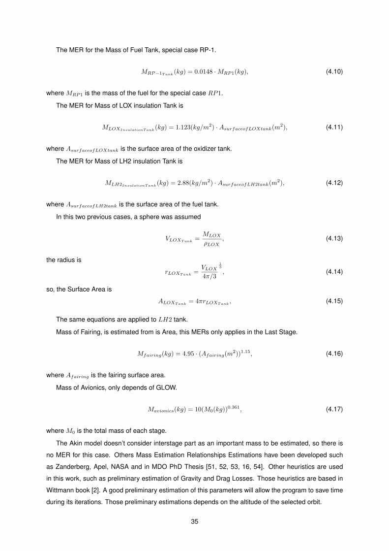
The MER for the Mass of Fuel Tank, special case RP-1.

MRP−1Tank(kg) = 0.0148 ·MRP1(kg), (4.10)

where MRP1 is the mass of the fuel for the special case RP1.

The MER for Mass of LOX insulation Tank is

MLOXInsulationTank(kg) = 1.123(kg/m2) ·AsurfaceofLOXtank(m2), (4.11)

where AsurfaceofLOXtank is the surface area of the oxidizer tank.

The MER for Mass of LH2 insulation Tank is

MLH2InsulationTank(kg) = 2.88(kg/m2) ·AsurfaceofLH2tank(m2), (4.12)

where AsurfaceofLH2tank is the surface area of the fuel tank.

In this two previous cases, a sphere was assumed

VLOXTank=MLOX

ρLOX, (4.13)

the radius is

rLOXTank=VLOX4π/3

13

, (4.14)

so, the Surface Area is

ALOXTank= 4πrLOXTank

, (4.15)

The same equations are applied to LH2 tank.

Mass of Fairing, is estimated from is Area, this MERs only applies in the Last Stage.

Mfairing(kg) = 4.95 · (Afairing(m2))1.15, (4.16)

where Afairing is the fairing surface area.

Mass of Avionics, only depends of GLOW.

Mavionics(kg) = 10(M0(kg))0.361, (4.17)

where M0 is the total mass of each stage.

The Akin model doesn’t consider interstage part as an important mass to be estimated, so there is

no MER for this case. Others Mass Estimation Relationships Estimations have been developed such

as Zanderberg, Apel, NASA and in MDO PhD Thesis [51, 52, 53, 16, 54]. Other heuristics are used

in this work, such as preliminary estimation of Gravity and Drag Losses. Those heuristics are based in

Wittmann book [2]. A good preliminary estimation of this parameters will allow the program to save time

during its iterations. Those preliminary estimations depends on the altitude of the selected orbit.

35

∆Vgravity = 0.08 < Vorbit < 0.12 (4.18)

∆Vdrag = 0.008 < Vorbit < 0.012 (4.19)

The initial values selected were ∆Vgravity = 0.12 · Vorbit and ∆Vdrag = 0.009 · Vorbit, because those

were the values that most decreased the velocity of the simulations.

Other Heuristic, for the same variables, but depending on Initial T/W .

∆Vgravity = 81.006

(T

W

)2

− 667.62

(T

W

)+ 1505.4 (4.20)

∆Vdrag = −32.692

(T

W

)2

+ 258.86

(T

W

)− 226.57 (4.21)

This different approach, shows us how the gravity and drag losses, depend on TW . The faster the

rocket flies in the dense atmosphere the drag losses will also increase. But on other hand for a lower

value of TW , the rocket will take more time to escape from the strong gravitational force from the Earth

and more time to achieve the target orbit. This approach can’t be used in our mass model because as

its going to be explained in the next chapter the mass model receives as input a ∆Vestimate and only

after the mass model was run, the initial value of TW is calculated 2.

2https://www.open-aerospace.org/rocket-sizing

36

Chapter 5

Rocket Design Tool

A tool was developed to help the preliminary design of a rocket. In this difficult task some design

parameters were selected as input and others were calculated from the selected ones. The values and

the variation of the input parameters were selected by the user.

The computer simulation program was designed to perform a rocket optimization. This means that it

optimizes all the masses and the dimensions of the vehicle as well as the last part of the trajectory. To

develop this work a Matlab code was developed, in order to design the rocket and simulate trajectories

into orbit.

There is the possibility to optimize performance by minimizing the take-off mass of the launch system,

for a given payload and target orbit. However, minimum take-off mass does not necessarily mean

minimum costs, and minimum costs might be the costs for a single mission or those of the complete life

cycle of the system, including development.

5.1 Program Overview

The program was divided in two main parts: first, the mass model and second, the trajectory. They were

developed separately, but depending on each other for complete design of a launch vehicle.

The mass model together with the trajectory will get the minimum GLOW and maximum payload ratio

for the purposed objectives (orbit altitude and payload mass), depending on user’s choices (Number of

Stages, Boosters, Propellant, Diameter, Thrust and Nozzle Area Ratio for each stage and ∆V Division)

and the variation of these parameters. For each combination of parameters all the masses and dimen-

sions are defined and then the trajectory will give the best trajectory that suits the configuration designed

before. The program achieves the final configuration when the ∆V used in mass model matches the

∆V of the trajectory. For each combination of parameters a minimum GLOW is calculated. After all

simulations done, the program selects the combination of parameters that achieve a minimum GLOW.

37

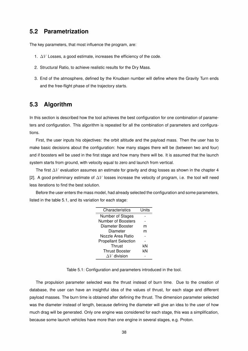
5.2 Parametrization

The key parameters, that most influence the program, are:

1. ∆V Losses, a good estimate, increases the efficiency of the code.

2. Structural Ratio, to achieve realistic results for the Dry Mass.

3. End of the atmosphere, defined by the Knudsen number will define where the Gravity Turn ends

and the free-flight phase of the trajectory starts.

5.3 Algorithm

In this section is described how the tool achieves the best configuration for one combination of parame-

ters and configuration. This algorithm is repeated for all the combination of parameters and configura-

tions.

First, the user inputs his objectives: the orbit altitude and the payload mass. Then the user has to

make basic decisions about the configuration: how many stages there will be (between two and four)

and if boosters will be used in the first stage and how many there will be. It is assumed that the launch

system starts from ground, with velocity equal to zero and launch from vertical.

The first ∆V evaluation assumes an estimate for gravity and drag losses as shown in the chapter 4

[2]. A good preliminary estimate of ∆V losses increase the velocity of program, i.e. the tool will need

less iterations to find the best solution.

Before the user enters the mass model, had already selected the configuration and some parameters,

listed in the table 5.1, and its variation for each stage:

Characteristics UnitsNumber of Stages -

Number of Boosters -Diameter Booster m

Diameter mNozzle Area Ratio -

Propellant Selection -Thrust kN

Thrust Booster kN∆V division -

Table 5.1: Configuration and parameters introduced in the tool.

The propulsion parameter selected was the thrust instead of burn time. Due to the creation of

database, the user can have an insightful idea of the values of thrust, for each stage and different

payload masses. The burn time is obtained after defining the thrust. The dimension parameter selected

was the diameter instead of length, because defining the diameter will give an idea to the user of how

much drag will be generated. Only one engine was considered for each stage, this was a simplification,

because some launch vehicles have more than one engine in several stages, e.g. Proton.

38

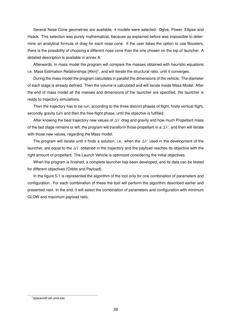
Several Nose Cone geometries are available, 4 models were selected: Ogive, Power, Ellipse and

Haack. This selection was purely mathematical, because as explained before was impossible to deter-

mine an analytical formula of drag for each nose cone. If the user takes the option to use Boosters,

there is the possibility of choosing a different nose cone than the one chosen on the top of launcher. A

detailed description is available in annex A.

Afterwards, in mass model the program will compare the masses obtained with heuristic equations

i.e. Mass Estimation Relationships [Akin]1, and will iterate the structural ratio, until it converges.

During the mass model the program calculates in parallel the dimensions of the vehicle. The diameter

of each stage is already defined. Then the volume is calculated and will iterate inside Mass Model. After

the end of mass model all the masses and dimensions of the launcher are specified, the launcher is

ready to trajectory simulations.

Then the trajectory has to be run, according to the three distinct phases of flight, firstly vertical flight,

secondly gravity turn and then the free-flight phase, until the objective is fulfilled.

After knowing the best trajectory new values of ∆V drag and gravity and how much Propellant mass

of the last stage remains or left, the program will transform those propellant in a ∆V , and then will iterate

with those new values, regarding the Mass model.

The program will iterate until it finds a solution, i.e. when the ∆V used in the development of the

launcher, are equal to the ∆V obtained in the trajectory and the payload reaches its objective with the

right amount of propellant. The Launch Vehicle is optimized considering the initial objectives.

When the program is finished, a complete launcher has been developed, and its data can be tested

for different objectives (Orbits and Payload).

In the figure 5.1 is represented the algorithm of the tool only for one combination of parameters and

configuration. For each combination of these the tool will perform the algorithm described earlier and

presented next. In the end, it will select the combination of parameters and configuration with minimum

GLOW and maximum payload ratio.

1spacecraft.ssl.umd.edu

39

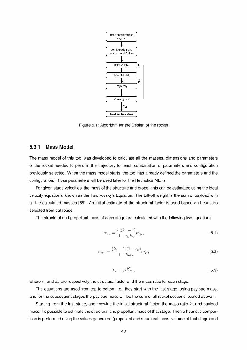
Figure 5.1: Algorithm for the Design of the rocket

5.3.1 Mass Model

The mass model of this tool was developed to calculate all the masses, dimensions and parameters

of the rocket needed to perform the trajectory for each combination of parameters and configuration

previously selected. When the mass model starts, the tool has already defined the parameters and the

configuration. Those parameters will be used later for the Heuristics MERs.

For given stage velocities, the mass of the structure and propellants can be estimated using the ideal

velocity equations, known as the Tsiolkovsky’s Equation. The Lift-off weight is the sum of payload with

all the calculated masses [55]. An initial estimate of the structural factor is used based on heuristics

selected from database.

The structural and propellant mass of each stage are calculated with the following two equations:

msn =εn(kn − 1)

1− εnknmpl, (5.1)

mpn =(kn − 1)(1− εn)

1− knεnmpl, (5.2)

kn = e∆V

gIspn , (5.3)

where εn and kn are respectively the structural factor and the mass ratio for each stage.

The equations are used from top to bottom i.e., they start with the last stage, using payload mass,

and for the subsequent stages the payload mass will be the sum of all rocket sections located above it.

Starting from the last stage, and knowing the initial structural factor, the mass ratio kn and payload

mass, it’s possible to estimate the structural and propellant mass of that stage. Then a heuristic compar-

ison is performed using the values generated (propellant and structural mass, volume of that stage) and

40

the parameters that are previously defined (thrust and nozzle area ratio). The Heuristic mass generated

will provide a new structural factor, then the program iterates using this new value. The program will stop

when the iteration of the structural factor converges with a maximum tolerance of 0.1%. This will define

the last stage. Now, the program has the conditions to estimate the masses of next stage, where the

mass of the payload will be the sum of masses of everything above. The same process is applied until

all masses are defined. In the last stage, the model adds a percentage of the propellant calculated, for

propellant reserve.

When the user chooses to use boosters during the first stage, there only is two solid propellants

available. The user will select two ∆V , one for the ”zeroth” stage considering the boosters and first

stage burning simultaneously and one only for the first stage, after the boosters were discarded. Two

is the minimum number of boosters to use and their burning time will be tested in the range 20% to

40% of the burning time of the first stage. After defining Thrust, with its burning time and the iteration of

structural ratio, all the parameters are defined. A specific heuristic comparison for boosters is performed

to validate the configuration.

In order to get appropriate dimensions for the Launcher, all the main dimensions are calculated.

For each iteration of structural factor in mass model, a new propellant mass is generated. Knowing

the density of propellant, we’re in conditions to know the volume and calculate the involving structure for

each stage. The volume of each stage will be 1.10 ·Vtanks, the diameter for each stage is already defined

so assuming a cylinder the length is calculated. Then, given a defined thickness for the structure and a

density for the alloy, an estimate of the mass external structure of each stage is calculated and added to

the heuristic structural mass [1].

MStruct = ρalloySth, (5.4)

where ρalloy is the density of the alloy, S the surface Area, and th the thickness of the structure. The

vehicle skin thickness must be as low as possible. A search for an heuristic of radius to wall thickness

was made, but there isn’t enough information available about this specific subject. The values of these

parameters are resumed in the table below:

ρalloy 2.7 g/cm3

t 33 mm

Table 5.2: Parameters of the Exterior Structure [2] [3].

The figure 5.2 shows the iterative process of how the mass model calculates the propellant and

structural masses for each stage (rocket section mass), where the ∆V is the ∆V assigned for the

specific stage.

41

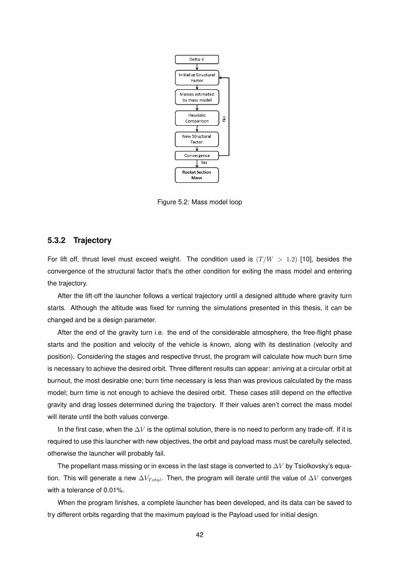
Figure 5.2: Mass model loop

5.3.2 Trajectory

For lift off, thrust level must exceed weight. The condition used is (T/W > 1.2) [10], besides the

convergence of the structural factor that’s the other condition for exiting the mass model and entering

the trajectory.

After the lift-off the launcher follows a vertical trajectory until a designed altitude where gravity turn

starts. Although the altitude was fixed for running the simulations presented in this thesis, it can be

changed and be a design parameter.

After the end of the gravity turn i.e. the end of the considerable atmosphere, the free-flight phase

starts and the position and velocity of the vehicle is known, along with its destination (velocity and

position). Considering the stages and respective thrust, the program will calculate how much burn time

is necessary to achieve the desired orbit. Three different results can appear: arriving at a circular orbit at

burnout, the most desirable one; burn time necessary is less than was previous calculated by the mass

model; burn time is not enough to achieve the desired orbit. These cases still depend on the effective

gravity and drag losses determined during the trajectory. If their values aren’t correct the mass model

will iterate until the both values converge.

In the first case, when the ∆V is the optimal solution, there is no need to perform any trade-off. If it is

required to use this launcher with new objectives, the orbit and payload mass must be carefully selected,

otherwise the launcher will probably fail.

The propellant mass missing or in excess in the last stage is converted to ∆V by Tsiolkovsky’s equa-

tion. This will generate a new ∆VTotal. Then, the program will iterate until the value of ∆V converges

with a tolerance of 0.01%.

When the program finishes, a complete launcher has been developed, and its data can be saved to

try different orbits regarding that the maximum payload is the Payload used for initial design.

42

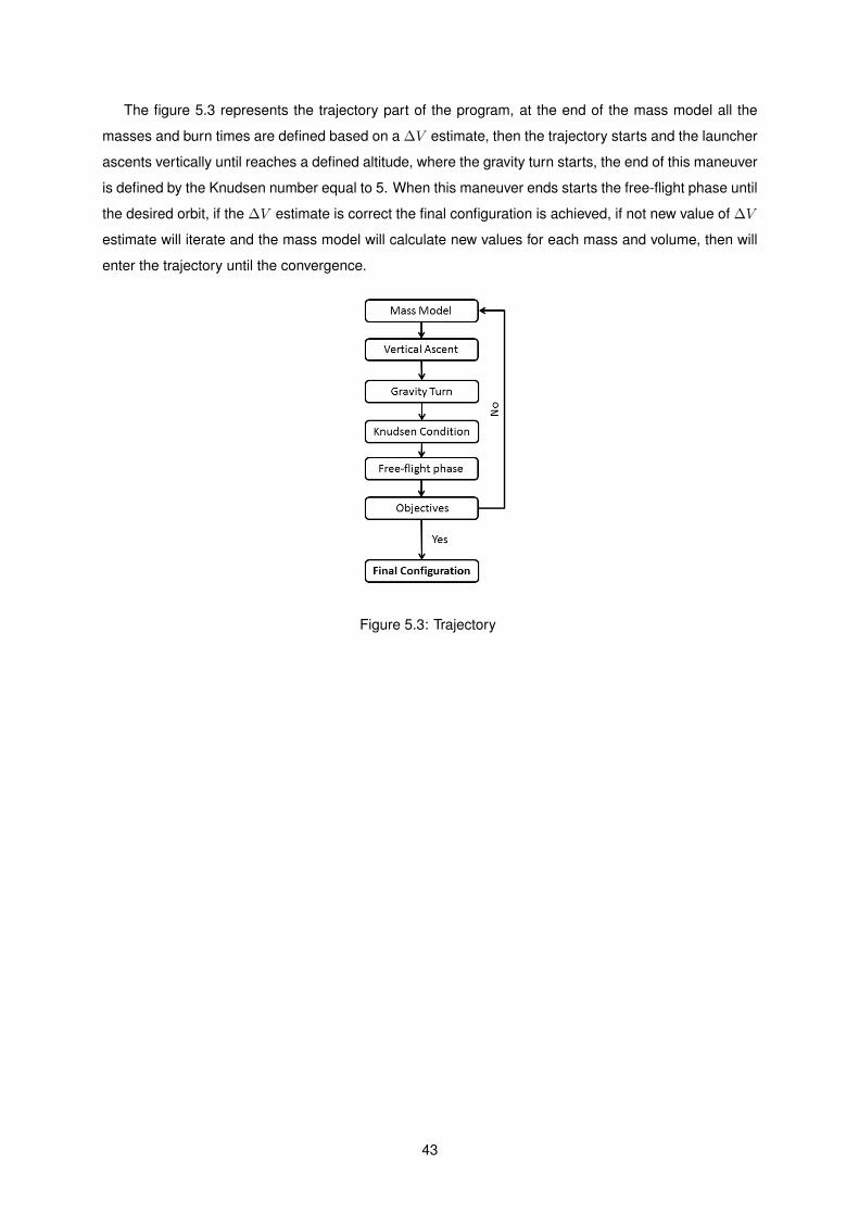
The figure 5.3 represents the trajectory part of the program, at the end of the mass model all the

masses and burn times are defined based on a ∆V estimate, then the trajectory starts and the launcher

ascents vertically until reaches a defined altitude, where the gravity turn starts, the end of this maneuver

is defined by the Knudsen number equal to 5. When this maneuver ends starts the free-flight phase until

the desired orbit, if the ∆V estimate is correct the final configuration is achieved, if not new value of ∆V

estimate will iterate and the mass model will calculate new values for each mass and volume, then will

enter the trajectory until the convergence.

Figure 5.3: Trajectory

43

Chapter 6

Results

In this chapter a comparison of the results obtained by the program and with those provided by the user’s

manual was performed. Two different launchers were compared: Vega and Proton K. Posteriorly, a set

of simulations was made, for the preliminary design and optimization of a new launcher, using as initial

parameters the values of Ariane 5. The optimization was based on the variation of some of the original

parameters and the result was a new launcher, an optimized Ariane 5.

6.1 Validation

Before using the tool for its purpose, its validation was necessary. It was performed in two separated

phases, starting with the validation of the trajectory and ending with the validation of the mass model.

The main objective of the simulation with Vega launcher was to place 1500 kilograms of payload into a

circular orbit, at an altitude of 700 kilometres, and the main objective of the Proton K was to place 19360

kilograms of payload in a circular orbit at an altitude of 200 kilometres.

The procedures followed include, first, testing the trajectory, i.e. if it achieves the objectives proposed,

and then running the entire program to compare the results obtained.

6.1.1 Trajectory

To validate the trajectory, firstly, a simulation was done with each launcher, using the specific character-

istics (thrust, burn time, diameter, propellant and structural masses) of Vega and Proton K, to confirm if

it managed to use the proposed trajectory. The principal characteristics of Vega launcher are presented

in the table 6.1 and the principal characteristics of the Proton K/DM3 are presented in the table 6.2 .

45

- 1 Stage 2 Stage 3 Stage 4 StageEngine P80 Zefiro 23 Zefiro 9 AVUM

Propellant Mass [kg] 88365 23906 10115 367Structural Mass [kg] 7431 1845 833 418

Propellant HTPB-Al/AP HTPB/AP HTPB/AP Hydrazine/NTOIsp [s] 280 289 294 317

Thrust [kN] 2092 959 230 2.2Burn Time [s] 105 71 116 620Diameter [m] 3 1.9 1.9 2.6

Nozzle Area Ratio 16 25 60.8 110

Table 6.1: Vega Launcher - Main characteristics [4]

Vega is an example of a newly developed small launcher. Initiated by the Italian Space Agency

(ASI), Vega became an ESA development program. It’s a three-stage solid propellant launch system

with an orbit injection module using storable liquid propellants. It’s launched from Guiana Space Center

(CSG) near Kourou, French Guiana. After third stage separation at the sub-orbital trajectory, the multiple

AVUM burns are used to transfer the payload to a wide variety of intermediate or final orbits, providing

the required plane changes and the orbit raising.

- 1 Stage 2 Stage 3 Stage 4 StageEngine RD-253 - 6 RD-0210 - 4 RD-0212 4 vernier RD-0214

Propellant Mass[kg] 419410 156113 46562 15200Structural Mass[kg] 30590 11717 4185 3150

Propellant UDMH/NTO UDMH/NTO UDMH/NTO LOX/KeroseneIsp[s] 316 289 327 353Thrust 3492 2328 582 87

Burn Time 120 327 230 600Diameter[m] 7.4 4.1 4.1 4

Nozzle Area Ratio 25 40 55 80

Table 6.2: Proton K/DM3 - Main characteristics [5].

Proton was, besides Ariane 5, the most important Launcher for lifting commercial payloads. Proton

is a four-stage Launcher operated from the Baikonur launch site in Russia. The first three stages are

propelled by storable liquids with identical engines that differ only in the length of their nozzle extensions.

Alternatively, Block D with a semi-cryogenic propulsion system or the Breeze upper stage, which can

be reignited up to 20 times, can be used as the fourth stage. Considering that the first stage has a

non-usual configuration, the Drag model was maintained but to achieve more realistic results a new

approach for Drag need to be applied for these configurations. In this simulation, Proton K don’t use its

upper stage DM-3. This simulation will assume the 4th stage as extra-Payload for re-insertion in other

orbit.

After the lift-off the vehicle ascends vertically up to 500 meters where the gravity turn starts. This

maneuver takes place until the effect of atmospheric conditions are negligible. To finish the GT and start

the free-flight phase where TPBVP happens the launcher has to be in exo-atmospheric conditions, this

means that the Knudsen number condition was achieved. The final times obtained at the end of the

trajectory was lower than the sum of all burning and coast times, and in the last stage 34% and 38%

46

respectively of the propellant mass wasn’t burned, meaning that the trajectory used was considered

validated for this two launchers.

Many simulations of GT were run during the development of this work. It’s possible to conclude that

the gravity losses during Atmospheric flight are larger, in their maximum value, than the ones foreseen by

the heuristics presented in chapter 4, that happens mainly because the launchers using this maneuver

spend more time inside atmospheric conditions than the trajectories usually used by launchers. On the

other hand the drag losses are smaller, this may occur by two conditions, the Cd model used produces

underestimated results or the velocity of the launcher during the atmosphere is smaller than in the

commonly trajectories.

6.1.2 Mass model validation

After the successful validation of the trajectory for each launcher. It’s time to perform the validation of

the mass model and of the entire tool.

The parameters introduced in the tool for the two simulations are presented in the table 6.3, all the

parameters were equal as the ones presented in respective user’s manual.

Characteristics UnitsNumber of Stages -

Number of Boosters -Nose Cone Selection -

Diameter Booster mDiameter m

Nozzle Area Ratio mPropellant Selection -

Thrust kNThrust Booster kN

∆V division -

Table 6.3: Configuration and parameters introduced in the tool

Subsequently, if the mass model converge, the trajectory is used once again to search for improve-

ments regarding the trajectory phase, i.e. reducing or increasing the propellant mass of the last stage,

transforming this mass in ∆V value and iterate the new values of ∆V losses. As explained before, this

change in the last stage mass will affect the other stages.

The total flight time was 357, 4 seconds and all the coast times are fixed to 3 seconds. The Knudsen

number condition was achieved at 97.1 seconds where the Gravity Turn ends and then starts the free-

flight phase.

The different variables, as propellant and structural mass, have been compared with the values

presented in Vega User’s Manual, and are presented in the table 6.4.

The expression used for the deviation of the results is

Deviation% =|Theoretical − Simulated|

Theoretical× 100, (6.1)

47

where the theoretical values were obtained in the user’s manual and the simulated ones with the tool.

Stage 1 Stage 2 Stage 3 Stage 4mp ms m0 mp ms m0 mp ms m0 mp ms m0

[kg] [kg] [kg] [kg] [kg] [kg] [kg] [kg] [kg] [kg] [kg] [kg]Vega 88365 7431 132530 23906 1845 36734 10115 833 10983 367 418 785

Simulation 83211.3 8595 126085 22918 2396.134248.9 8566.2 906.2 11663.8 516.6 175.6 2192.2Deviation % 5.83 15.6 4.8 4.1 29.8 6.8 15.3 8.1 6.1 40.7 57.6 11.8

Table 6.4: Mass Model Comparison - Vega

The most significant differences were obtained in Structural mass, specially in the second stage

where the difference was almost 30%. The structural and propellant mass of last stage are the ones that

have more differences, specially the structural mass because last stage usually have ”more structure”,

i.e. more avionics, wiring and a complicated thrust attitude controller for the re-ignitions, so the MERs

used in Mass model doesn’t have the same accuracy for upper stages as they have for lower stages.

The program overestimates all the structural masses but on the other hand the propellant masses

calculated were inferior with the exception of the last stage once again, that can be explained by the fact

that the last stage of the original launcher have multiple burns and long coast times and that analysis

isn’t provided in the trajectory. The difference in the others stages are explained for the non existence

of the propellant margin. The biggest difference in the propellant masses excluding last stage was in

third stage with a difference of 15.3%. The GLOW was a difference of 4.8%, that is inferior to 10% for a

tool of preliminary design the differences are relatively small. The Payload mass was added to the last

stage. The mass model was considered validated for this case.

The results of the dimensions achieved for the launcher are presented in the table 6.5.

Stage 1 Stage 2 Stage 3 Stage 4d l V d l V d l V d l V[m] [m] [m3] [m] [m] [m3] [m] [m] [m3] [m] [m] [m3]

Vega 3 11.2 79.1 1.9 8.39 23.8 1.9 4.12 11.7 2.2 2 7.6Simulation 3 10.6 74.9 1.9 8 22.7 1.9 3.7 10.5 2.2 1.5 6.7

Deviation % - 5.4 5.3 - 4.6 4.6 - 10.2 10.3 - 25 11.8

Table 6.5: Volume Comparison - Vega

All the dimensions were inferior to the original Vega. That happens because the propellant masses

of each stage were inferior compared with the original launcher, due to the definition of the total volume

of each stage being an overestimation of the volume of the Propellant tanks. Although the difference in

the volume, the effect in overall length is almost negligible.

A comparison between the flight performance/trajectory presented in the User’s Manual, and the

trajectory obtained by the code, was done. The results were considerably different, due to the fact that

the trajectory uses a pure gravity turn and modern launchers now use powerful and effective guidance

models. Also, the model assumes constant and maximum thrust in all stages but in real launchers, thrust

isn’t always at full power and sometimes, reverse thrust is used for the accommodation of payload and

astronauts.

The following figures show different variables of the trajectory simulation. Only in two are represented

48

all the parts of flight. In the other figures, it’s more difficult to see the first phase of the flight, it’s only

possible to observe the second and third phases. The Gravity Turn ends when the flight time was 97.1

seconds and after that the launcher starts to raise faster to the desired orbit. The total flight time was

357.4 seconds.

In the figure 6.1 its presented the evolution of the Altitude with time, after the end of GT the launcher

starts to accelerates and velocity increases. In the figure 6.1 its presented the evolution of the altitude

vs downrange of the trajectory.

(a) Altitude vs Time - Vega (b) Altitude vs Downrange - Vega

Figure 6.1: Vega Launcher Simulation

It’s possible to observe, in fig 6.2(a) the Flight Path Angle, divided in three separate phases, first the

vertical ascent phase where the FPA doesn’t change, second gravity turn and then the free-flight phase.

In the figure 6.2(b) it’s possible to observe the velocity function of time and the change after the end of

gravity turn.

(a) Flight Path Angle vs Time - Vega (b) Velocity vs Time - Vega


In the figure 6.3(a) is represented the Altitude as a function of Velocity, where is possible to observe

the end of GT and the start of the free-flight phase. In the figure 6.3(a) the Dynamic Pressure is repre-

sented. This value is very important in the design phase for Structural strength and reliability of Fairing

during the first part of the trajectory. The maximum occurs around 9 km of altitude, that was assumed

correct because the maximum usually occurs around an altitude of 10 km.

49

(a) Altitude vs Velocity - Vega (b) Dynamic Pressure - Vega


After the validation of the mass model and the tool with the small launcher Vega, we proceed with

the simulations with Proton K launcher.

The parameters used to input in the program were the same as in Vega simulation, they are pre-

sented in the table 6.2.

The total flight time to orbit was 509.2 seconds. The two coast phases are equal to Vega simulation,

3 seconds each. The Gravity Turn starts at an altitude of 500 meters. The altitude where the free-flight

phase started was higher than the Vega simulation because the diameter of last stage of Proton is higher

than the Vega, which means that Proton needs to raise higher to achieve exo-atmospheric conditions

defined by Knudsen Number.

The mass model results are presented in table 6.6.

Stage 1 Stage 2 Stage 3mp ms m0 mp ms m0 mp ms m0

[kg] [kg] [kg] [kg] [kg] [kg] [kg] [kg] [kg]PROTON K 419410 30590 668577 156113 11717 218577 46562 4185 50747Simulation 1 395390 36563 626563 142878 12323 194610 34127 5282 39409Deviation % 5.7 19.5 6.3 8.5 5.2 11 26.7 26.2 22.3

Table 6.6: Mass Model Comparison - PROTON K

Once again, the mass variables are compared between the user’s manual information and the results

obtained by the tool. All the propellant masses calculated were inferior than the original Launcher, being

the biggest difference in the last stage and the smallest in the first stage. The differences are explained

by the non existence of the propellant margin. The structural mass calculated was always superior than

the real Launcher: the biggest difference was in the last stage and the smallest was in the second stage.

The GLOW had a difference of 6.2%. For a tool of preliminary design the differences are relatively small

and the mass model was considered validated for this case.

All the dimensions results are presented in table 6.7.

The values were inferior compared with Proton K original, because the propellant masses of each

stage were inferior compared with the original Launcher and the definition of the total volume of each

stage is an overestimation of the volume of the propellant tanks. The differences in the Volume are larger

in upper stages being around 24%, but the effect in overall length is, once again, almost negligible.

50

Stage 1 Stage 2 Stage 3d l V d l V d l V[m] [m] [m3] [m] [m] [m3] [m] [m] [m3]

Proton K 7.4 21.2 911.3 4.1 14.39 190 4.1 6.5 85.8Simulation 7.4 20.1 864 4.1 13.3 175.5 4.1 4.9 64.7Deviation - 5.2 5.2 - 7.6 7.6 - 24.6 24.6

Table 6.7: Volume Comparison - Proton K

A comparison between the trajectory obtained by the code and the flight performance/trajectory

presented in the Users Manual can’t be performed because the flight performance wasn’t available in

the user’s manual.

The following figures show different variables of the trajectory simulation. Only in two figures all the

parts of flight are represented. In the other figures, it’s more difficult to see the first phase of the flight,

it’s only possible to observe the second and third phases. The Gravity Turn ends at 153 seconds and

after that the launcher starts to raise to the desired orbit. The total flight time was 509.2 seconds. Here,

the payload achieves its desired orbit with 5% of propellant reserve.

In figure 6.4(a) its represented the Altitude of the trajectory vs time. In the figure 6.4(b) is represented

the altitude vs downrange, it’s possible to observe in both figures that the payload reaches the desired

orbit.

(a) Altitude vs Time - Proton K (b) Altitude vs Downrange - Proton K

Figure 6.4: Proton K Launch Simulation

In the figure 6.5(a) its represented the Flight Path Angle vs time, divided in three distinct phases, first

the vertical ascent, then Gravity Turn until the end of considerable atmosphere and at last the free-flight

phase until the desired orbit. The figure 6.5(b) represents velocity of Launcher vs time, where it’s also

possible to observe the end of GT and the start of the free-flight phase and how the launcher rapidly

ascents to the desired orbit.

51

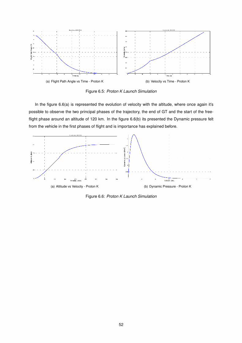
(a) Flight Path Angle vs Time - Proton K (b) Velocity vs Time - Proton K


In the figure 6.6(a) is represented the evolution of velocity with the altitude, where once again it’s

possible to observe the two principal phases of the trajectory, the end of GT and the start of the free-

flight phase around an altitude of 120 km. In the figure 6.6(b) its presented the Dynamic pressure felt

from the vehicle in the first phases of flight and is importance has explained before.

(a) Altitude vs Velocity - Proton K (b) Dynamic Pressure - Proton K


52

6.2 Preliminary Design and Optimization

In the last case, a set of simulations was done with the objectives of Ariane 5 for LEO, an altitude of

200 km and a payload mass of 19.3 tons, but in this simulation some parameters were varied with the

goal of obtaining an optimal configuration, this means the minimum GLOW that can satisfied the desired

objectives.

The Ariane 5 is a 2.5-stage launch system primarily used for lifting heavy satellites to a GTO. Its

capability of launching two satellites totalling a maximum of 9 tons to GTO and 18 tons to LEO. Two

versions are operated today: A5E/CA with a cryogenic upper stage for launching commercial payloads

and A5ES-ATV for lifting the ATV supply vehicle to the ISS. The upper stage of this version is re-ignitable

and uses storable liquid propellants. Both versions use a cryogenic first stage and two large solid

propellant boost stages. Ariane 5 is launched from the European CSG spaceport near Kourou in French

Guiana.

The principal characteristics of the Ariane 5 are presented in the table 6.8.

- Boosters 1 Stage 2 StageEngine EAP EPC 23 ESC-A

Propellant Mass [kg] 480000 170000 14900Structural Mass [kg] 80000 14700 4540

Propellant HTPB −Al/AP LOX + LH2 LOX + LH2

Isp [s] 274.5 432 446Thrust [kN] 14000 1390 67

Burn Time [s] 129 537 972Diameter [m] 3 5.4 5.4

Nozzle Area Ratio 30 57 88

Table 6.8: Ariane 5 Launcher - Main characteristics.

Three groups of different simulations were run. In the first group, the diameter and thrust of each

stage were fixed but on the other hand the number of boosters and its characteristics, thrust, diameter

and burn time were varied in a certain range. In parallel with the first group simulation, the second group

simulation was run with all the parameters fixed except the diameter of core stages. The third group

simulation used the best result of the first group simulation for the boosters (its thrust and dimensions)

and the best diameter obtained in the second group simulation with the variation of ∆V division and

respective thrust for each stage. In the end, an optimal solution was found and its configuration was the

one with minimum GLOW that achieves the objectives early proposed. A total of 170 simulations were

run and a total of seven parameters were varied and its variation it’s represented in the table 6.9.

53

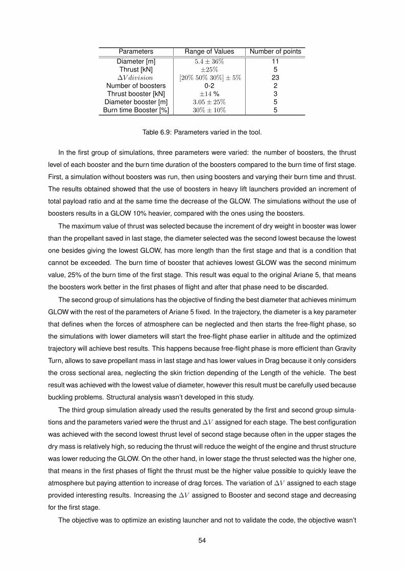
Parameters Range of Values Number of pointsDiameter [m] 5.4± 36% 11Thrust [kN] ±25% 5

∆V division [20% 50% 30%]± 5% 23Number of boosters 0-2 2Thrust booster [kN] ±14 % 3

Diameter booster [m] 3.05± 25% 5Burn time Booster [%] 30%± 10% 5

Table 6.9: Parameters varied in the tool.

In the first group of simulations, three parameters were varied: the number of boosters, the thrust

level of each booster and the burn time duration of the boosters compared to the burn time of first stage.

First, a simulation without boosters was run, then using boosters and varying their burn time and thrust.

The results obtained showed that the use of boosters in heavy lift launchers provided an increment of

total payload ratio and at the same time the decrease of the GLOW. The simulations without the use of

boosters results in a GLOW 10% heavier, compared with the ones using the boosters.

The maximum value of thrust was selected because the increment of dry weight in booster was lower

than the propellant saved in last stage, the diameter selected was the second lowest because the lowest

one besides giving the lowest GLOW, has more length than the first stage and that is a condition that

cannot be exceeded. The burn time of booster that achieves lowest GLOW was the second minimum

value, 25% of the burn time of the first stage. This result was equal to the original Ariane 5, that means

the boosters work better in the first phases of flight and after that phase need to be discarded.

The second group of simulations has the objective of finding the best diameter that achieves minimum

GLOW with the rest of the parameters of Ariane 5 fixed. In the trajectory, the diameter is a key parameter

that defines when the forces of atmosphere can be neglected and then starts the free-flight phase, so

the simulations with lower diameters will start the free-flight phase earlier in altitude and the optimized

trajectory will achieve best results. This happens because free-flight phase is more efficient than Gravity

Turn, allows to save propellant mass in last stage and has lower values in Drag because it only considers

the cross sectional area, neglecting the skin friction depending of the Length of the vehicle. The best

result was achieved with the lowest value of diameter, however this result must be carefully used because

buckling problems. Structural analysis wasn’t developed in this study.

The third group simulation already used the results generated by the first and second group simula-

tions and the parameters varied were the thrust and ∆V assigned for each stage. The best configuration

was achieved with the second lowest thrust level of second stage because often in the upper stages the

dry mass is relatively high, so reducing the thrust will reduce the weight of the engine and thrust structure

was lower reducing the GLOW. On the other hand, in lower stage the thrust selected was the higher one,

that means in the first phases of flight the thrust must be the higher value possible to quickly leave the

atmosphere but paying attention to increase of drag forces. The variation of ∆V assigned to each stage

provided interesting results. Increasing the ∆V assigned to Booster and second stage and decreasing

for the first stage.

The objective was to optimize an existing launcher and not to validate the code, the objective wasn’t

54

to see if the results match but how different will be the new optimized launcher compared with the original

Ariane 5, how lighter will be, and how the volume will vary. The values achieved for the best configuration

are presented in the table 6.10.

Parameters Final ValueDiameter [m] 3.9Thrust [kN] 1700 and 58.5

∆V division [%] [25% 49% 26%]Number of boosters 2Thrust booster [kN] 8000

Diameter booster [m] 2.625Burn time Booster [%] 25%

Table 6.10: Optimal Configuration Achieved.

The total flight time to orbit was 462.8 seconds. The coast phase is equal to Vega and Proton K

simulation, 3 seconds. The Gravity Turn starts at an altitude of 500 meters. The altitude where the

free-flight phase started was higher than the Vega’s and almost the same altitude of the Proton K’s

simulations because the diameter of last stage simulated was 3.9 meters, meaning that the optimized

launcher needs to raise up to 120 kilometres to achieve exo-atmospheric conditions.

First, the different masses are compared between the user’s manual information and the results

obtained by the last simulation. The results are presented in the table 6.11.

Booster Stage 1 Stage 2mp ms m0 mp ms m0 mp ms m0

[kg] [kg] [kg] [kg] [kg] [kg] [kg] [kg] [kg]Ariane 5 480000 80000 764140 170000 14700 204140 14900 4540 19440

Simulation 458189.4 77216 680076.5 123735 14406 144671.1 2217 4313 6530Deviation % 4.5 3.5 11 27.2 2 29.1 85.1 5 66.4

Table 6.11: Mass Model Comparison - Ariane 5

In this optimization all the propellant masses calculated were smaller than the ones from the original

Launcher, the biggest difference being in the last stage and the smallest around in the booster stage.

Comparing this differences, with those obtained for the validations of the model it’s possible to state that

optimization of the parameters decrease the propellant necessary to achieve the orbit. The structural

masses calculated were slightly inferior than the ones from the real Launcher: the biggest difference

was in the second stage and the smallest happened in first stage. These difference can be explained

by the reduction of the mass of the propellant and its direct influence in decreasing the mass of the

propellant tanks.

The goal of this optimization was the reduction of GLOW, the final simulation had a difference of

11%, which allows to reduce 84 tons the weight of the Launcher at lift-off and compared with the other

simulations, where the objective was to validate the code, it possible to say that the original Ariane 5

was optimized and consequently its GLOW reduced.

The dimensions obtained are presented in the table 6.12. The values were inferior compared with

Ariane 5 original because the propellant masses of each stage were inferior due to optimization.

55

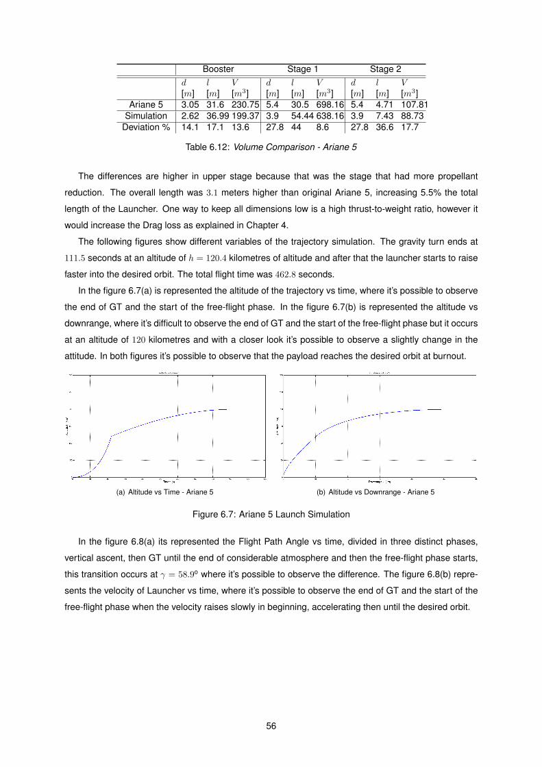
Booster Stage 1 Stage 2d l V d l V d l V[m] [m] [m3] [m] [m] [m3] [m] [m] [m3]

Ariane 5 3.05 31.6 230.75 5.4 30.5 698.16 5.4 4.71 107.81Simulation 2.62 36.99 199.37 3.9 54.44 638.16 3.9 7.43 88.73

Deviation % 14.1 17.1 13.6 27.8 44 8.6 27.8 36.6 17.7

Table 6.12: Volume Comparison - Ariane 5

The differences are higher in upper stage because that was the stage that had more propellant

reduction. The overall length was 3.1 meters higher than original Ariane 5, increasing 5.5% the total

length of the Launcher. One way to keep all dimensions low is a high thrust-to-weight ratio, however it

would increase the Drag loss as explained in Chapter 4.

The following figures show different variables of the trajectory simulation. The gravity turn ends at

111.5 seconds at an altitude of h = 120.4 kilometres of altitude and after that the launcher starts to raise

faster into the desired orbit. The total flight time was 462.8 seconds.

In the figure 6.7(a) is represented the altitude of the trajectory vs time, where it’s possible to observe

the end of GT and the start of the free-flight phase. In the figure 6.7(b) is represented the altitude vs

downrange, where it’s difficult to observe the end of GT and the start of the free-flight phase but it occurs

at an altitude of 120 kilometres and with a closer look it’s possible to observe a slightly change in the

attitude. In both figures it’s possible to observe that the payload reaches the desired orbit at burnout.

(a) Altitude vs Time - Ariane 5 (b) Altitude vs Downrange - Ariane 5

Figure 6.7: Ariane 5 Launch Simulation

In the figure 6.8(a) its represented the Flight Path Angle vs time, divided in three distinct phases,

vertical ascent, then GT until the end of considerable atmosphere and then the free-flight phase starts,

this transition occurs at γ = 58.9o where it’s possible to observe the difference. The figure 6.8(b) repre-

sents the velocity of Launcher vs time, where it’s possible to observe the end of GT and the start of the

free-flight phase when the velocity raises slowly in beginning, accelerating then until the desired orbit.

56

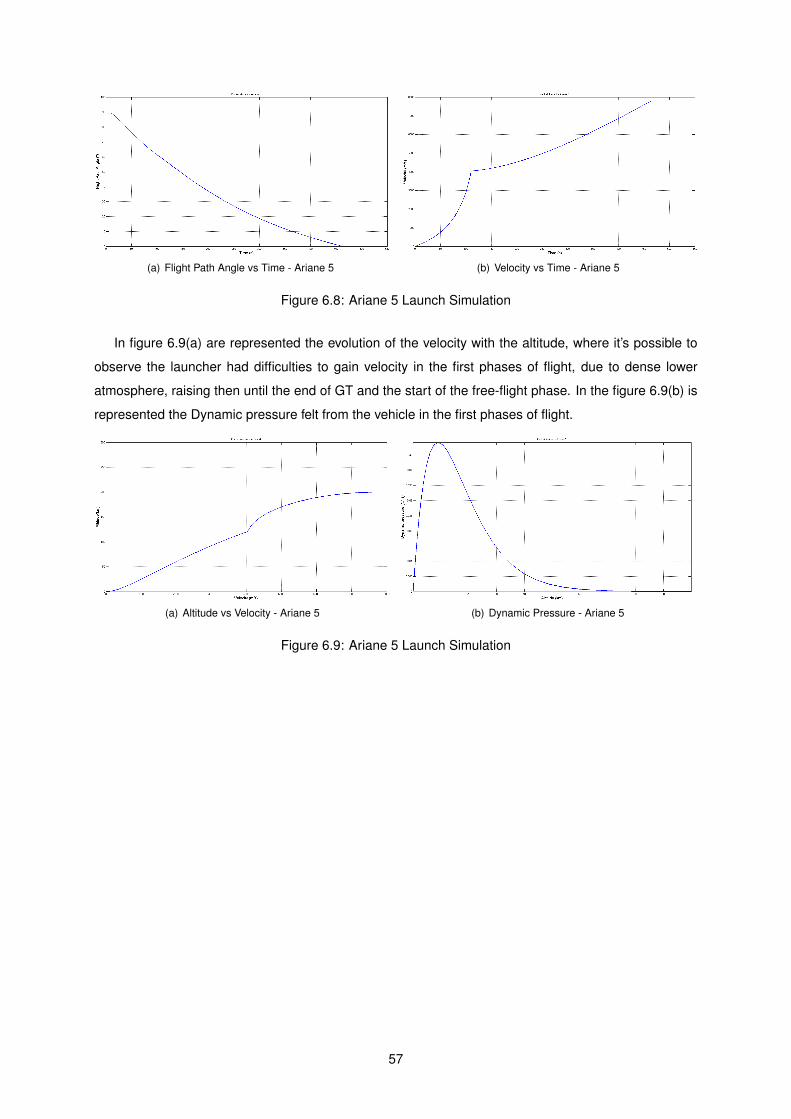
(a) Flight Path Angle vs Time - Ariane 5 (b) Velocity vs Time - Ariane 5


In figure 6.9(a) are represented the evolution of the velocity with the altitude, where it’s possible to

observe the launcher had difficulties to gain velocity in the first phases of flight, due to dense lower

atmosphere, raising then until the end of GT and the start of the free-flight phase. In the figure 6.9(b) is

represented the Dynamic pressure felt from the vehicle in the first phases of flight.

(a) Altitude vs Velocity - Ariane 5 (b) Dynamic Pressure - Ariane 5


57

Chapter 7

Conclusions

The main goal of this research was to develop a tool to assist the preliminary design of rockets. The

tool was modelled using a MATLAB code, which applies a simplified optimization, and covers two major

fields: the mass model and the trajectory.

The database created during this study allowed the understanding of some important variables, such

as length, diameter, thrust, burning time, specific masses and others, providing their range of values and

ensuring the viability of the final result. Some of these values were used in the mass model, as initial

structural factors, for the iteration of the mass model, such as the fairing mass, estimated from GLOW

and the respective volume, to accommodate the payload. An effort to create MERs was done, but

the lack and dispersion of information available about the specific mass of the components, made this

estimation almost impossible to perform. Nonetheless, MERs were estimated, concerning fairing.

The mass model created, showed that the use of Tsiolkovsky’s equation with the MERs heuristics,

provides realistic results for the structural masses of the launcher. The structural factor iterates until it

finds convergence with the MERs heuristics and the design is made from top to bottom. This model also

calculates the dimensions of the launcher, with the goal of adding more realism to the final design; the

weight of the external structure of each stage is estimated by the definition of volumes. When the mass

model is concluded, all the masses needed for the trajectory model (propellant and structural mass) and

dimensions of the launcher have been defined. This is important, because the diameter of the last stage

is one of the conditions to define the Knudsen number.

The trajectory was divided into three distinct phases. Initially, after the lift-off, the launcher rises

vertically until a certain altitude, the value used for the simulations was 500 m, but it can be optimized.

After this, it starts the gravity turn, which ends when the atmosphere affects are negligible, condition

defined by the Knudsen number. When the launcher achieves exo-atmospheric conditions, it starts the

free-flight phase, which will minimize the time, and consequently, the propellant used. The atmospheric

model used is a combination of the US standard atmosphere of 1962 and 1976 valid up to an altitude of

2000 kilometres. A simplified drag model was used, where the Cd only varies with Mach number. The

same happens for gravity model where the gravity only varies with altitude.

When the program is concluded, a new Launcher has been designed and all the masses and di-

59

mensions have been defined. In this phase, new objectives can be tested, taking into account that the

maximum payload is the designed one and that the orbits must be carefully selected.

The Model validation is important to determine the accuracy of the results obtained. In this study, the

model validation was done regarding two examples, Vega and Proton K, targeting different objectives

(Orbit and Payload Mass) and characterised by different configurations. Both validations were done with

the values presented in the user’s manual. First, an isolated simulation of the trajectory was done, i.e.

using the mass values from the user’s manual, the launcher achieves the desired objectives. Both sim-

ulations were successful, achieving the desired orbit with some propellant mass of the last stage in their

tanks. The difference between both results and their user’s manual can be explained by the assumption

of constant and maximum thrust in every stage and for the completely burnout of the propellant mass

assumed in the tool, which doesn’t correspond to the real way launchers operate.

After the validation of the trajectory, it was possible to validate the mass model. All the parameters

selected for the design were fixed and were the same of the respective User’s manual. The results

showed that almost all the propellant masses were inferior, when compared to real launchers, explained

by the fact that the mass model only adds propellant margin for the last stage, instead of adding it for all

stages. The structural masses were almost all superior, when compared with real launchers, meaning

the mass model is over estimating the structural weight for the selected launchers. The GLOW of each

launcher was inferior, and that is explained by the reasons presented for the deviation regarding the

propellant masses. Almost all the dimensions were inferior compared to the user’s manual, because of

the dependency of the total volume of the propellant mass, since the densities of the propellants were

the same.

After the validation of the developed tool, this was used for the preliminary design of a rocket. The

original parameters used were based on launcher Ariane 5, and some were modified, to optimize the

rocket i.e. increase the payload ratio by reducing the GLOW. This allowed the understanding of which

parameters influence more the difficult task of designing a rocket. The objectives of the mission were

the same as those defined for Ariane 5 (orbit and payload mass) and in the end of the optimization

all masses and dimensions were compared with the user’s manual. All the masses were inferior; the

propellant masses differences can be explained by the non-existence of propellant margin and also by

the reduction of the diameter, which allowed the free-flight phase to start earlier; the structural masses

were also inferior because of the reduction of all propellants masses, the lighter tanks and the reduction

of the diameter, which decreased the weight of the structure and allowed the free-flight phase of the

trajectory to start earlier, optimizing the fuel consumption. In conclusion, the reduction of GLOW was

significant, meaning that the optimization was successful.

The ∆V division and thrust are the parameters that most influence the GLOW. The definition of

diameter effects drag and trajectory because of the definition of the Knudsen number and must be

carefully selected, due to the fact that in this study a structural analysis wasn’t developed. The use

of boosters increased the payload ratio, i.e. the payload mass increases for the same GLOW, and this

effect is more significant in medium and heavy launchers. The burning time of boosters must be reduced

to allow a rapid discard of the mass of its empty tanks.

60

As a conclusion, a tool to assist the design, and improve the configuration of a space launch vehicle,

was created. Its validation was done comparing the results obtained with Vega and Proton K launchers.

The results indicate that the program can be used as a starting point in the difficult task of designing

earth launch vehicles. The set of simulations performed with Ariane 5 demonstrated that this tool can

also be used as an optimizer, for already existing configurations. By varying some parameters it is

possible to obtain a whole new configuration, for the objectives earlier defined.

7.1 Future Work

Below are presented some ideas for future developments, to allow further studies on this subject.

• Implement a Guide User Interface (GUI), that will allow users to run the program without requiring

knowledge of the language of the code.

• Include the chamber pressure and the Nozzle areas in the Mass model. Currently its effect is

neglected on the nozzle mass, defining the pressure at exit to improve the thrust model with Nozzle

Area Ratio.

• Implement a more realistic Mass model for the engine. If mass only depends on Thrust, i.e. if the

engine increases its efficiency, its mass will also increase.

• Improve the Drag model. A more realistic Drag model can be achieved with analytical equations

for each Nose Cone Configuration. The use of other Software like DATCOM cannot be discarded.

• Implement constrains in the Trajectory model, such as Max. Dynamic Pressure, Heat Flux, Bend-

ing Load and Axial Acceleration. Some of this values are already calculated in the program, so a

thrust vector control have to be created. This will provide a more realistic trajectory.

• Develop more options for Boosters, defining various types of Grain Geometry, special nose cones

and increase the available solid propellants used in the Code.

• Implement some changes to air launched rockets (Pegasus) and to those launched with inclination,

for safety reasons, like in Japan.

• Develop a Cost Model, or use an existing one, in order to obtain a realistic insight of Launch Vehicle

Design.

• Design transfer orbits to GEO and interplanetary trajectories, with the improvement of the Guid-

ance Model to perform long Coast Phases.

• Include dis-alignment Thrust vector in ∆V Losses, the effect of the Earth’s non-spherical gravita-

tional field and the effect of gravity from other bodies (Moon and Sun).

• Rewrite the program in C or C++ will decrease the time necessary to complete the simulations.

61

Bibliography

[1] George P. Sutton. Rocket Propulsion Elements. 8 edition, 2010.

[2] Willi Hallmann Klaus Wittmann and Wilfried Ley. Handbook of Space Technology. Wiley, 2009.

[3] NASA. Space Shuttle User’s Manual, 2008.

[4] Arianespace. VEGA User’s Manual, 2006.

[5] PROTON Launch System Mission Planner’s Guide, 2001.

[6] National Aeronautics. Rockets - A Teacher’s Guide, 1999.

[7] Frank H. Winter, Michael J. Neufeld, and Kerrie Dougherty. Was the rocket invented or accidentally

discovered? Some new observations on its origins. Acta Astronautica, 77:131–137, August 2012.

[8] Alan C. Tribble. A Tribble’s guide to Space. Princeton, 2000.

[9] Jim Winchester. Space Missions. Amber, 2006.

[10] Willam E. Wiesel. Spaceflight Dynamics. Aphelion, third edition edition, 2010.

[11] E. Civek-Coskun and Kemal Ozgoren. A generalized staging optimization program for space launch

vehicles. Recent Advances in Space Technologies (RAST), pages 857–862, 2013.

[12] Reza Jamilnia and Abolghasem Naghash. Simultaneous optimization of staging and trajectory of

launch vehicles using two different approaches. Aerospace Science and Technology, 23(1):85–92,

2012.

[13] R D Braun and A A Moore. Collaborative Approach to Launch Vehicle Design. Journal of Spacecraft

and Rockets, 34(4), 1997.

[14] Amer Farhan Rafique, He LinShu, Ali Kamran, and Qasim Zeeshan. Multidisciplinary design of air

launched satellite launch vehicle: Performance comparison of heuristic optimization methods. Acta

Astronautica, 67(7-8):826–844, October 2010.

[15] Lawrence F Rowell, Robert D Braun, and John R Oldst. Multidisciplinary Conceptual Design Opti-

mization of Space Transportation Systems. Journal of Aircraft, 36(1), 1999.

63

[16] Mathieu Balesdent, Nicolas Berend, Philippe Depince, and Abdelhamid Chriette. A survey of mul-

tidisciplinary design optimization methods in launch vehicle design. Structural and Multidisciplinary

Optimization, 45(5):619–642, September 2011.

[17] R. D. Braun, R. W. Powell, R. a. Lepsch, D. O. Stanley, and I. M. Kroo. Comparison of two multi-

disciplinary optimization strategies for launch-vehicle design. Journal of Spacecraft and Rockets,

32(3):404–410, May 1995.

[18] Young Chang Choi, Kyung-Ho Noh, Jae-Woo Lee, Yung-Hwan Byun, and Bong-Kyo Park. Optimal

air-launching rocket design using system trades and a multi-disciplinary optimization approach.

Aerospace Science and Technology, 13(7):406–414, October 2009.

[19] Rizwan Ullah, De-qun Zhou, Peng Zhou, Mukarrum Hussain, and M Amjad Sohail. An approach

for space launch vehicle conceptual design and multi-attribute evaluation. Aerospace Science and

Technology, 25(1):65–74, 2013.

[20] David R. Greatrix. Powered Flight - The Engineering of Aerospace Propulsion. Springer, 2012.

[21] Fernando Alonso Zotes and Matilde Santos Penas. Multi-criteria genetic optimisation of the ma-

noeuvres of a two-stage launcher. Information Sciences, 180(6):896–910, March 2010.

[22] Emanuele Di Sotto and Paolo Teofilato. Semi-Analytical Formulas for Launcher Performance Eval-

uation. Journal of Guidance, Control, and Dynamics, 25(3), 2002.

[23] Ping Lu and Binfeng Pan. Highly Constrained Optimal Launch Ascent Guidance. Journal of Guid-

ance, Control, and Dynamics, 33(2):404–414, March 2010.

[24] Nicolas Berend and Christophe Talbot. Overview of some optimal control methods adapted to ex-

pendable and reusable launch vehicle trajectories. Aerospace Science and Technology, 10(3):222–

232, April 2006.

[25] Greg A Dukeman, Nasa Marshall, Space Flight, and Ashley D Hill. Rapid Trajectory Optimization

For the ARES I Launch Vehicle. Technical Report August, 2008.

[26] D. M. Azimov. Active Rocket Trajectory Arcs: A Review. Automation and Remote Control,

66(11):1715–1732, November 2005.

[27] John T. Betts. Survey of Numerical Methods for Trajectory Optimization. Journal of Guidance,

Control, and Dynamics, 21(2):193–207, March 1998.

[28] E. Trelat. Optimal Control and Applications to Aerospace: Some Results and Challenges. Journal

of Optimization Theory and Applications, 154(3):713–758, April 2012.

[29] Max Cerf, Thomas Haberkorn, and Emmanuel Trelat. Continuation from a flat to a round Earth

model in the coplanar orbit transfer problem. Optimal Control Applications and Methods, 2011.

[30] Takeshi Tsuchiya. Optimal Conceptual Design of Two-Stage Reusable Rocket. Journal of Space-

craft and Rockets, 41(5), 2004.

64

[31] Michael Thierschmann. SSTO applications based on super high energy propulsion systems. Acta

Astronautica, 22:219–227, 1990.

[32] H.D. Froning Jr and Huntington Beach. Investigation of very high energy rocket for future SSTO

vehicles. Acta Astronautica, 19(4):321–330, 1989.

[33] Dietrich E. Koelle. Economics of Small fully Reusable Launch Systems. Acta Astronautica,

40(2):535–544, 1991.

[34] Martin J. Bayer. Analytic performance considerations for lifting ascent trajectories of winged launch

vehicles. Acta Astronautica, 54(10):713–721, May 2004.

[35] Ashish Tewari. Atmospheric and Space Flight Dynamics. Birkhauser, 2006.

[36] Claire Ballard. Conceptual Lay-out of a Small Launcher. Master’s thesis, 2012.

[37] Jack D Mattingly and Hans Von Ohain. Elements of Propulsion : Gas Turbines and Rockets. AIAA,

2006.

[38] Joseph Z. Ben-Asher. Optimal Control Theory with Aerospace Applications. 2010.

[39] Sighard F. Hoerner. Fluid-Dynamic Drag. Hoerner Fluid Dynamics, 1965.

[40] Ashish Tewari. Advanced Control of Aircraft, Spacecraft and Rockets. Wiley, 2011.

[41] American Institute of Aeronautics and Astronautics. American National Standard Guide to Refer-

ence and Standard Atmosphere Models. Technical report, 2009.

[42] Eurockot. Rockot User’s Guide, 2011.

[43] Orbital. Pegasus User’s Guide, 2007.

[44] SpaceX. Falcon 1 Launch Vehicle Payload User ’ s Guide, 2008.

[45] Arianespace. SOYUZ User’s Manual, 2006.

[46] SLLP. Zenit User’s Guide, 2000.

[47] United Launch Alliance. Delta IV Launch Services User’s Guide. United Launch Alliance, 2013.

[48] Arianespace. Ariane 5 User’s Manual, 2011.

[49] United Launch Alliance. Atlas V Launch Services User’s Guide. United Launch Alliance, 2010.

[50] B. T. C. Zandbergen. AE1222-II : Aerospace Design Systems Engineering Elements I Part :

Launcher design and sizing .

[51] Reuben R Rohrschneider. Development of a Mass Estimating Relationship Database for Launch

Vehicle Conceptual Design. Technical report, 2002.

[52] Willie Heinemun Jr. NASA Technical Note fundamental techniques of weight estimating and fore-

casting for advanced manned spacecraft and space stations. Technical Report May, 1971.

65

[53] P.J. Klich. NASA Technical Memorandum of Mass Properties of Earth-To-Orbit Transportation Sys-

tems. Technical report, 1978.

[54] Francesco Castellini. Multidiscplinary Design Optimization for Expendable Launch Vehicles. PhD

thesis, Politecnico di Milano, 2012.

[55] Geethaikrishnan. Multi-Disciplinary design optimization strategy in multi-stage launch vehicle con-

ceptual design,. Department of Aeroespace Engineering Indian Institute of Technology, 2003.

[56] W. T. Thomson. Introduction to Space Dynamics. Dover, 1986.

[57] Howard Curtis. Orbital Mechanics for Engineering Students. Elsevier, 2005.

[58] Martin J. L. Turner. Rocket and Spacecraft Propulsion. Springer, third edition edition, 2009.

[59] Howard Curtis. Orbital Mechanics for Engineering Students. Elsevier, 2005.

[60] Jae-Woo Lee, Young-Ki Lee, Yung-Hwan Byun, and Ho-Yon Hwang. Design of Space Launch

Vehicle Using Numerical Optimization and Inverse Method. Journal of Spacecraft and Rockets,

38(2):212–218, March 2001.

[61] Amer Farhan Rafique, Linshu He, Ali Kamran, and Qasim Zeeshan. Hyper Heuristic Approach for

Design and Optimization of Satellite Launch Vehicle. Chinese Journal of Aeronautics, 24(2):150–

163, April 2011.

[62] Mathieu Balesdent, Nicolas Berend, Philippe Depince, and Abdelhamid Chriette. Multidisciplinary

Design Optimization of Multi-Stage Launch Vehicle using Flight Phases Decomposition. Interna-

tional Journal for Simulation and Multidisciplinary Design Optimization, 4(3-4):117–125, February

2012.

[63] Douglas J. Bayley, Roy J. Hartfield, John E. Burkhalter, and Rhonald M. Jenkins. Design Optimiza-

tion of a Space Launch Vehicle Using a Genetic Algorithm. Journal of Spacecraft and Rockets,

45(4):733–740, July 2008.

[64] L. Ridolfi, M. Pontani, and P. Teofilatto. Effect of different flight conditions at the release of a small

spacecraft from a high performance aircraft. Acta Astronautica, 66(5-6):665–673, March 2010.

[65] J Roshanian and Z Keshavarz. Multidisciplinary design optimization applied to a sounding rocket.

Journal Indian Institute, pages 363–375, 2006.

[66] Qasim Zeeshan, Dong Yunfeng, Khurram Nisar, Ali Kamran, and Amer Rafique. Multidisciplinary

Design and Optimization of Multistage Ground-launched Boost Phase Interceptor Using Hybrid

Search Algorithm. Chinese Journal of Aeronautics, 23(2):170–178, April 2010.

[67] S N Maitra. Constant thrust programming for a multistage rocket flown in vacuum with a given initial

T/W. 8(October):373–385, 1985.

66

[68] GA AIAA Space 2001 Conference and Exposition Albuquerque , New Mexico. AIAA 2001-4542 A

Comparison of Modern and Historic Mass Estimating Relationships on a Two-Stage to Orbit Launch

Vehicle , 2001.

[69] Mauro Pontani and Paolo Teofilatto. Acta Astronautica Simple method for performance evaluation

of multistage rockets. Acta Astronautica, pages 1–12, 2013.

[70] V Adimurthy and Vikram Sarabhai. Launch Vehicle Trajectory Optimization . Acta Astronautica,

15(11):845–850, 1987.

[71] Shashi Kant Shrivastava. Determination of optimal trajectory under design constraints for a satellite

launch vehicles. Acta Astronautica, 3(September):333–347, 1976.

[72] Donald J Estep, Dewey H Hodges, and Michael Warner. The solution of a launch vehicle trajec-

tory problem by an adaptive finite-element method. Computer Methods in Applied Mechanics and

Engineering, 190:4677–4690, 2001.

[73] NASA. Optimum Rocket Trajectories. 27(8):955–961, 1956.

[74] A Miele. Rocket Flight in a Resisting Medium I. Journal of Optimization Theory and applications,

(2).

[75] Glen J. Culler and Burton D. Fried. Universal Gravity Turn Trajectories. Journal of Applied Physics,

28(6):672, 1957.

[76] B D Fried, J M Richardson, and D F Lawden. General Formulation of Powered Flight Trajectory

Optimization Problems. Journal applied Physics, (v):1203–1209, 1958.

[77] G E Dorrington. Gravity-Turn Trajectories. 37(4):543–544, 1990.

[78] Mathieu Balesdent. OPTIMISATION MULTIDISCIPLINAIRE DE LANCEURS ( Multidisciplinary De-

sign Optimization of Launch Vehicles ). PhD thesis, Ecole Centrale de Nantes, 2011.

[79] T Miele, A and Wang. Multiple-Subarc Gradient-Restoration Algorithm, Part 2: Application to a

Multistage Launch Vehicle Design. Journal of Optimization Theory and Applications, 116(1):19–39,

2003.

67

Appendix A

Nose Cone Geometries

A.1 Nose Cone Geometries

There are several rocket nose cones, for this study four were considered: Ogive, Power, Ellipse and

Haack [39]. As explained previously in chapter 4, the nose cones are added as extra volume to the last

stage, resulting as fairing Volume. This volume is considered part of the total volume of the last stage.

A.1.1 Ogive

In the rocketry model, the most common ogive shape used is the tangent ogive, which is formed by the

radius of curvature of the circle ρt

ρt =R2 + L2

2R(A.1)

When the radius of curvature ρ is superior to ρt, the resulting nose cone has an angle at the joint

between the nose cone and body tube, and is called a secant ogive. At the limit the secant ogive

becomes a conical nose cone.

The parameter value k is the ratio of radius of curvature of a corresponding tangent ogive ρt to the

radius of curvature of the nose cone ρ:

k =ρtρ

(A.2)

k takes values from zero to one, where k = 1 produces a tangent ogive and k = 0 produces a conical

nose cone (infinite radius of curvature).

The radius of curvature is

ρ2 =(L2 +R2) · (((2− k)L)2 + (kR)2)

4(kR)2(A.3)

69

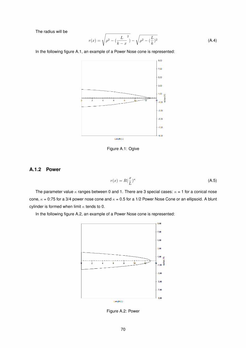
The radius will be

r(x) =

√ρ2 − (

L

k − x

2

)−√ρ2 − (

L

k)2 (A.4)

In the following figure A.1, an example of a Power Nose cone is represented:

Figure A.1: Ogive

A.1.2 Power

r(x) = R(x

L)κ (A.5)

The parameter value κ ranges between 0 and 1. There are 3 special cases: κ = 1 for a conical nose

cone, κ = 0:75 for a 3/4 power nose cone and κ = 0.5 for a 1/2 Power Nose Cone or an ellipsoid. A blunt

cylinder is formed when limit κ tends to 0.

In the following figure A.2, an example of a Power Nose cone is represented:

Figure A.2: Power

70

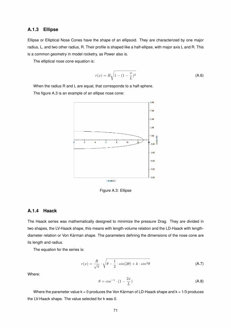
A.1.3 Ellipse

Ellipse or Elliptical Nose Cones have the shape of an ellipsoid. They are characterized by one major

radius, L, and two other radius, R. Their profile is shaped like a half-ellipse, with major axis L and R. This

is a common geometry in model rocketry, as Power also is.

The elliptical nose cone equation is:

r(x) = R

√1− (1− x

L)2 (A.6)

When the radius R and L are equal, that corresponds to a half-sphere.

The figure A.3 is an example of an ellipse nose cone:

Figure A.3: Ellipse

A.1.4 Haack

The Haack series was mathematically designed to minimize the pressure Drag. They are divided in

two shapes, the LV-Haack shape, this means with length-volume relation and the LD-Haack with length-

diameter relation or Von Karman shape. The parameters defining the dimensions of the nose cone are

its length and radius.

The equation for the series is:

r(x) =R√π·√θ − 1

2· sin(2θ) + k · sin3θ (A.7)

Where:

θ = cos−1 · (1− 2x

L) (A.8)

Where the parameter value k = 0 produces the Von Karman of LD-Haack shape and k = 1/3 produces

the LV-Haack shape. The value selected for k was 0.

71

The figure A.4 is an example of a Von Karman - Haack series nose cone:

Figure A.4: Haack

72

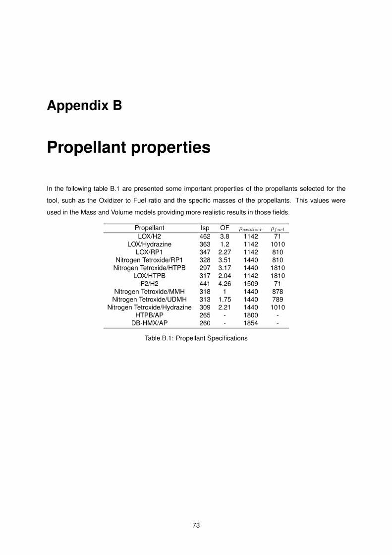
Appendix B

Propellant properties

In the following table B.1 are presented some important properties of the propellants selected for the

tool, such as the Oxidizer to Fuel ratio and the specific masses of the propellants. This values were

used in the Mass and Volume models providing more realistic results in those fields.

Propellant Isp OF ρoxidizer ρfuelLOX/H2 462 3.8 1142 71

LOX/Hydrazine 363 1.2 1142 1010LOX/RP1 347 2.27 1142 810

Nitrogen Tetroxide/RP1 328 3.51 1440 810Nitrogen Tetroxide/HTPB 297 3.17 1440 1810

LOX/HTPB 317 2.04 1142 1810F2/H2 441 4.26 1509 71

Nitrogen Tetroxide/MMH 318 1 1440 878Nitrogen Tetroxide/UDMH 313 1.75 1440 789

Nitrogen Tetroxide/Hydrazine 309 2.21 1440 1010HTPB/AP 265 - 1800 -

DB-HMX/AP 260 - 1854 -

Table B.1: Propellant Specifications

73

a tool for preliminary design of rockets - técnico lisboa · a tool for preliminary design of...

Documents