a. travel demand model - appalachian regional · pdf filematrix estimator (odme) procedure to...

Economic Impact Study of Completing the Appalachian Development Highway System

Cambridge Systematics, Inc. / Economic Development Research Group / HDR Decision Economics A-1

A. Travel Demand Model The purpose of the Appalachian Region Commission (ARC) travel demand model is to evaluate the future conditions upon completion of the Appalachian Development Highway System (ADHS). The proposed ADHS was evaluated using the ARC travel demand model to determine the impact on the travel per-formance. Highway projects such as adding capacity to a roadway, adding additional mileage of roadways, and relocation or removal of roadways were analyzed using the travel demand model.

Forecast travel demand models traditionally consist of four steps. During the first step, Trip Generation, the number of trips being produced and attracted to or by an area is estimated based on the land use of the area and generation rates which are usually derived from a survey. The second step, Trip Distribution, determines the number of trips from the Trip Generation step that are going between areas. The third step, Mode Split, predicts by which mode of transpor-tation the trips will occur. The final step, Trip Assignment, assigns the trips to a network that represents the modeled area.

The travel demand model developed for the ARC travel demand model is not a four-step model. The ARC travel demand model uses an Origin-Destination Matrix Estimator (ODME) procedure to estimate the trip tables used in the model. The ODME procedure replaces the traditional trip generation and distri-bution steps of the four-step modeling procedure. ODME is an accepted practice that estimates trip tables based on traffic count data. Traffic count data is gener-ally more readily available than the socioeconomic data that is required for trip generation, and since ODME does not need survey data to derive trip rates and lengths, the procedure is dramatically less costly to implement.

The mode split step in not included in the model. However, three different modes/purposes were used in the model. Trip tables were developed for auto-mobiles and trucks, with the truck being further classified as commodity-carrying trucks and non-commodity-carrying trucks.

The assignment step from the four-step model is used in a similar manner in the ARC travel demand model. Commodity and non-commodity trucks are assigned to the network together with automobile trip table in a multiclass congested equilibrium assignment.


A-2 Cambridge Systematics, Inc. / Economic Development Research Group / HDR Decision Economics

A.1 BACKGROUND The analysis for the completion of the ADHS requires forecasts of the traffic vol-umes on the all of the roadways in the ARC region that will vary in response to the ADHS improvement alternatives. While there is no travel demand model for the multistate Arc region, the basic functionality of such a model; i.e., trip tables and networks, were developed as part of this project. A highway network was being developed and trip tables were being estimated from observed traffic counts using an origin-destination matrix estimation (ODME) technique. The TransCAD travel demand modeling software used in this study has an ODME feature available as a standard option.

A.2 MODEL DEVELOPMENT A.2.1 Highway Network A TransCAD highway network for the United States was developed as part of FHWA’s Freight Analysis Framework – Version 1 (FAF1)22 project. It provides basic infrastructure and connectivity information for major highways in the United States. The FAF1 highway network of the United Sates uses counties as loading points.

This highway network includes sufficient detail to analyze the ADHS perform-ance. It includes highway throughout the United States, far beyond the bounda-ries of the ARC region. The FAF1 highway network includes automobile and truck traffic counts on all links in the highway system. Those traffic counts are those reported by the state department of transportation, primarily through the FHWA’s Highway Performance Monitoring System. The HPMS submittals also provide lane, speed, and capacity information that were included in the FAF1 network. Only major roads were included in the highway network model.

The boundaries chosen for the ARC travel demand model highway network, was selected to include not only the highways in the ARC region, but the major highway decision points, for example the interstate highways nearby the ARC region, where a traveler could chose to use or not use a route involving an improved ADHS road, based on the quality of service that was being provided. Therefore, rather than just the 417 counties (and incorporated cities in Virginia) as TAZs in the model, and a total of 697 counties are included as TAZs in the model, 280 of which are in a “halo” of TAZs/counties within the model bound-ary but outside the ARC region. The highway network includes not only 23,042 miles of intestates and other major highways within the ARC region but 76,634 22 Battelle Memorial Institute, Freight Analysis Framework Highway Capacity Version 1:

Methodology Report, Office of Freight Management and Operations, Federal Highway Administration, April 18, 2002.


Cambridge Systematics, Inc. / Economic Development Research Group / HDR Decision Economics A-3

miles outside of the ARC region for a total of 99, 676 miles of major highways in the entire model area.

At the edge of the model region, 125 external stations were coded to provide for travel between these external stations and the remainder of the United States. The inclusion of these stations allows the inclusion of automobile and truck trips that travel from the rest of the United States to the ARC model TAZs, to the rest of the United States from the ARC model TAZs, or from the western United Stets to the eastern United States passing through the highway in the Arc model region.

A.2.2 Trip Tables Absent a traditional “four-step” model covering the ARC region, including the “halo” of counties surrounding the Arc region, an alternative method had to be identified to develop base year trip tables. The Origin Destination Matrix Estimation technique implemented in TransCAD was used for this purpose. This technique builds the statistically most likely trip table that is consistent with the highway network and its observed traffic counts. This feature is included as a standard feature in TransCAD. The method is improved with the use of a “seed” trip table. An unvalidated “seed” table was created by applying standard national trip generation rates to the base year socioeconomic data in the model and then distributing those trips based on the average highway travel times between TAZs in the model using a standard gravity model trip distribution.

When assigned to the highway network, the base year trip table will produce average daily trips between counties and the external stations that match the average daily traffic counts. Separate counts were provided for trucks and autos. This information was used to estimate separate automobile and truck trip tables.

The truck trip table is based on observed truck volumes, which include both freight and non-freight trucks. The 2002 FAF2 commodity freight truck table was allocated from FAF2 regions to the ARC model counties using the county percentages by commodity from a 1998 commodity flow freight database developed for ARC by Marshall University. This table includes additional detail about the contents of those freight trucks. These commodity tables were subtracted from the original ODME truck table. This will result in an automobile trip table, a non-freight truck trip table, and additional freight truck trip tables by commodity.

A.2.3 Assignment The trip tables can be assigned to the highway network in a conventional manner using the congestion on the highway links to determine the shortest paths. Changes in the physical attributes of the highway system can be coded and used to test how traffic volumes will change in response to highway improvements. A terrain code was added to all roads in the Arc highway network which charac-terizes the highway section as “flat,” “rolling,” or “mountainous.” That terrain


A-4 Cambridge Systematics, Inc. / Economic Development Research Group / HDR Decision Economics

code was based on average terrain in the county. Before calculating congested speeds a Passenger Car Equivalent of 1.5, 2.5, or 4.5, for flat, rolling and moun-tainous terrain respectively was applied to the assigned volume of trucks prior to comparing the total volume on the highway to the capacity of highways when the congested speed is computed. The congested speeds are used in an equilib-rium assignment that ensures that each vehicle traveling between two zones ahs the same congested travel time, regardless of which route is chosen.

A.2.4 Forecast Trip Tables The estimated trip tables are prepared independently of trip generation and dis-tribution steps so these steps cannot be used to produce forecasts. Forecast trip tables are produced by factoring the estimated trip table based on changes in county-level employment and population. Standard trip generation rates were applied to the Global Insight (medium- growth scenario) 2020 and 2035 popula-tion and employment and for the Woods and Poole (high-growth scenario) 2020 and 2035 population and employment forecasts. Those rates were applied to the base automobile and non-commodity freight truck trip tables using the ratio of the base and future control totals by county using an Iterative Proportional Fitting technique (i.e., Fratar). The future freight truck table was developed by allocating the FAF2 2020 and 2035 trip tables in exactly the same manner that the base year commodity trip table was created.

A.2.5 Future Assignments The development of future year trip tables together with the existing and future highway networks provided the ability to forecast future highway volumes for those future networks. The No-Build highway network was created by updating the base year network with ARC “Cost to Complete” GIS database. That data-base was used to identify ADHS improvement that have been completed or will be completed by others, in addition to ADHS projects where construction is committed by ARC. Those projects define the No-Build highway network. Those ADHS project for which funding has not yet been secured are part of the Build scenario. The ARC “Cost to Complete” GIS database was used to deter-mine the proposed number of lanes and the proposed design speed for widen section of ADHS highway, and the design and location of new roads.


Cambridge Systematics, Inc. / Economic Development Research Group / HDR Decision Economics B-5

B. Market Access and Economic Development Impacts Modeling Section 2.5 summarized the methodology for estimating economic development benefits, using the Transportation Economic Development Impact System (TREDIS). This appendix presents additional information regarding that methodology. It is organized into three parts: 1) process for analysis of market access changes and business attraction impacts, 2) description of market access changes, and 3) analysis of economic impact timing and magnitude.

B.1 MARKET ACCESS IMPACT METHODOLOGY B.1.1 Process for Estimating Market Access Benefit This section expands upon the description of the market access impact analysis process that was provided in Section 2.5.2 of the main report. In summary, this process estimates the extent of new economic activity created by changes in transportation connectivity and access – effects that are beyond the traditional “travel efficiency benefit” measures of travel time, cost, and safety changes. It covers two types of transportation changes created by completion of the ADHS:

(A) Impacts from expanded market reach, facilitating agglomeration economies (i.e., operational efficiencies associated with working in larger markets); and

(B) Impacts from enhanced intermodal connectivity, resulting from either enhanced service levels or enhanced connectivity to those services.

For each county within Appalachia, market reach change is measured in terms of size of the labor market (measured as population accessible within 60 minutes of the county population center), and size of the same-day truck delivery market (measured in terms of employment within three hours one-way truck delivery time from the county populations center). Intermodal connectivity is measured in terms of the change in travel times from each county to the nearest commercial airport, marine port, intermodal rail facility and international freight gateway.

The methodology for estimating market access impacts in TREDIS is drawn from the Local Economic Assessment Package (LEAP) economic development analysis process. Impacts are estimated at the county level based on the access change variables, shown above. The steps are as follows.

First, the groups of ARC counties are compared to non-ARC counties in the same states to determine whether the extent to which they exhibit “gaps” in economic


B-6 Cambridge Systematics, Inc. / Economic Development Research Group / HDR Decision Economics

mix or growth performance. This gap analysis is performed at the industry level. Second, the relative strengths and weaknesses of transport and non-transport factors are assessed. This step identifies whether any economic development potential in the study area can be achieved by improving access factors (as, say, improving the quality of the labor force). After the potential benefit from improving transport access is identified, the market access module utilizes the inputs shown above to determine the extent of the access improvements. This leads to the final step of estimating the magnitude of economic development impact.

The magnitude of the impact is determined by cross-referencing three “pools” of data. These are: 1) the mix of industry observed in the study area; 2) each industry’s utilization of and sensitivity to different modes in select markets; and 3) the extent of improvement of these modal accessibilities. The markets consid-ered in the present study include the labor market, final demand consumer mar-kets, supply-chain delivery markets, and markets for international imports and exports.

B.1.2 Multiregion Applications: Net and Gross Impacts The Market Access module is based on the theory that locational advantage strengthens an area’s potential for conducting business. In practice, given a change in access to markets, subsequent growth may reflect either local produc-tivity gains or relocation of productive activity from other areas (or some combi-nation thereof). Activity shifts may reflect actual firm migration or local industrial expansion coupled with contraction elsewhere. This can include shifts from outside areas to the Appalachian region, or shifts within the Appalachian region. Clearly, there is a need to adjust for the latter case to avoid double-counting of economic impacts.

In a multistate regional analysis as applied in this study, TREDIS accounts for potential offsets within the broader study area with a spatial adjustment module. This module distinguishes the extent to which business attraction and relocation occurs within the Appalachian region or from outside to the Appalachian region. This makes it possible to estimate the net economic develop-ment impact for the overall Appalachian region.

Rest of Country

Project Area

StudyRegions



B.1.3 Sources of Growth The spatial adjustment module is sensitive to several types of growth following an access-improving transportation investment. These fall into three categories: increased productivity, increased export activity, and relocation of productive factors.

First, an access improvement may raise the productivity of the directly affected region. In this category, we use the term “productivity” to mean the ratio of out-put per worker (as opposed to “expansion of output”). This productivity gain stems from the benefits of increased agglomeration. These positive externalities have been well-established in the literature,23 and reflect the mechanisms of bet-ter labor matching, better selection of intermediate inputs, and knowledge spill-overs. The ensuing productivity gains are realized as increased output and value added relative to employment. In other words, access (and resulting agglomera-tion) allows firms to make better use of existing labor and capital inputs without necessarily increasing local employment. As such, any local benefits from mar-ket access improvements do not necessarily come at the expense of other parts of the study area. In fact, research indicates that productivity gains from agglom-eration are more likely to have positive spatial externalities – that is, local gains may improve the economic performance of neighboring areas.

The second possible effect is a gain in industrial output (sales) through increased exports. Results are based on research relating exports (sales) to accessibility to different types of international gateways. As such, improvements in access may increase industrial output in the host region such that: 1) technology does not necessarily change – that is, the ratio of output and income to employment may remain constant; and 2) economic benefits to one region do not necessarily come at the expense of others, because the increased outputs helps satisfy international demand (which is assumed to be highly inelastic).

Finally, accessibility improvements may change the geography of profitability for spatially competitive firms. Access changes have the potential to increase revenue potential or decrease costs at a particular location relative to other loca-tions. The increased revenue potential may come from increased accessibility to consumers of a particular type; decreased costs may come from industrial or logistical reorganization capitalizing on access changes (these are distinct from travel-time and travel-cost savings). In either case, an access improvement may induce migration of productive factors to take advantage of the new economic landscape. The key point here is that the migration is due to relative cost changes between regions in spatial competition. In practice, this “migration” occurs over relatively long-time scales (5 to 10 years), and may be observed as either physical

23 For a review of the theory and empirics of agglomeration-productivity relationships,

see reviews by Rosenthal and Strange (2003), Puga (2003), Fujita and Thisse (2002), or Eberts and McMillen (1999).



relocation of a single business, through firm birth/death that benefits one region at the expense of another, or it could reflect the opening of branch offices in one location at the expense of another. In any of these cases, local economic growth comes at the expense of other competing jurisdictions, and, therefore, must be accounted for when considering the net impact to each in a multi-region project.

B.1.4 Adjusting for Spatial Relocation The Market Access module estimates the impacts due to each of the three effects described above separately. Because the first two effects are assumed to have no relocation impacts on neighboring areas, only the third impact type is used to determine net impacts to a group of distinct study regions. More specifically, the spatial accounting module estimates the spatial relocation of employment resulting from market access improvements that affect relative cost or revenue factors.

The module begins by considering the estimated economic development gains in employment to a “destination” area within the larger study region. These gross impact numbers reflect potential benefits to an area as though it were the only one impacted by a project. The destination area is then compared, in a pair-wise fash-ion, to all the other areas within the broader study region. For each pair, employment relocation is estimated from the “source” area to the “destination” area based on several factors (discussed below). After all interproject area pairs have been cycled through, the module moves to another “destination” area, and all pair-wise comparisons are performed again. This sequence is repeated for as many times as there are areas within the broader study region.

Each pair-wise comparison is made on an industry-specific basis. In other words, the module asks: “if the destination area is forecast to gain X jobs in a specific sector, then how many of those jobs may be drawn from the ‘origin’ area?” The result is based on several factors, including sector properties, the distance between the two areas, and the industry trends of the origin area.

Sector Properties – For any area-to-area pair within the broader region, the magnitude of relocation depends on the specific industry under considera-tion. This accounts for different levels of mobility among different types of production. For example, service sector firms are more mobile than manu-facturing firms because the latter are more capital intensive and, therefore, moving costs are higher. Furthermore, revenues for service firms are typi-cally more spatially dependent than manufacturing firms. Finally, industries that are nationally or globally serving may be less sensitive to cost differences between two areas. Other things equal, locally serving sectors are modeled as more mobile, and more likely to be drawn from nearby areas, whereas more nationally serving industries are modeled as less mobile, and as more likely to be drawn from anywhere in the area (rather than only nearby areas).



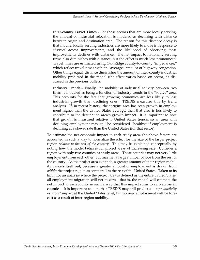
Inter-county Travel Times – For those sectors that are more locally serving, the amount of industrial relocation is modeled as declining with distance between origin and destination area. The reason for this distance decay is that mobile, locally serving industries are more likely to move in response to observed access improvements, and the likelihood of observing these improvements declines with distance. The net impact to nationally serving firms also diminishes with distance, but the effect is much less pronounced. Travel times are estimated using Oak Ridge county-to-county “impedances,” which reflect travel times with an “average” amount of highway congestion. Other things equal, distance diminishes the amount of inter-county industrial mobility predicted in the model (the effect varies based on sector, as dis-cussed in the previous bullet).

Industry Trends – Finally, the mobility of industrial activity between two firms is modeled as being a function of industry trends in the “source” area. This accounts for the fact that growing economies are less likely to lose industrial growth than declining ones. TREDIS measures this by trend analysis. If, in recent history, the “origin” area has seen growth in employ-ment higher than the United States average, then that area is less likely to contribute to the destination area’s growth impact. It is important to note that growth is measured relative to United States trends, so an area with declining employment may still be considered “healthy” if employment is declining at a slower rate than the United States (for that sector).

To estimate the net economic impact to each study area, the above factors are accounted in such a way to normalize the effect for the size of the larger project region relative to the rest of the country. This may be explained conceptually by noting how the model behaves for project areas of increasing size. Consider a region with only two counties as study areas. These counties may net very little employment from each other, but may net a large number of jobs from the rest of the country. As the project area expands, a greater amount of inter-region mobil-ity cancels itself out, because a greater amount of employment is drawn from within the project region as compared to the rest of the United States. Taken to its limit, for an analysis where the project area is defined as the entire United States, all employment migration will net to zero – that is, the model will estimate the net impact to each county in such a way that this impact sums to zero across all counties. It is important to note that TREDIS may still predict a net productivity or export impact at the United States level, but no new employment will be fore-cast as a result of inter-region mobility.



B.2 MARKET ACCESS INPUTS These tables provide summaries of the changes in market access from no-build to build. The amount in each cell is the number counties that fall into the corre-sponding category for each variable.

Table B.1 provides the change in the accessible markets by 2035 for ARC due to the improved highway access for the medium scenario.

Table B.1 Changes in Accessible Population (Number of Counties) by 2035 Medium Scenario (Global Insight)

Percentage Change Consumer/Labor Market (60 Minutes) Delivery Market (180 Minutes)

0% 335 97

<5% 11 215

5%-10% 14 34

10%-20% 18 25

20%-30% 7 18

>30% 25 21

Table B.2 provides the improvement in access time to all modes of transportation for counties in Appalachia for the medium scenario. The last column shows the number of counties that had the largest impact in terms of minutes for any given mode (for example: 37 counties received no improvement for access to any mode).

Table B.2 Changes in Mode Access (Number of Counties) by 2035 Medium Scenario (Global Insight)

Change in Access Time (Minutes)

International Gateway Rail Air Water

Largest Mode Change

0 94 117 152 137 37

< 5 Minutes 217 243 215 199 240

5 to 10 Minutes 34 13 14 14 20

10 to 20 Minutes 29 15 21 47 59

20 to 30 Minutes 25 7 6 10 30

>30 Minutes 11 15 2 3 24



Table B.3 shows the modes that had the largest impact – shown by the number of counties. This explains that while a majority of counties received a small impact on mode access; however, 119 counties had a mode access improvement greater than 10 minutes.

Table B.3 Largest Mode Access Change (Number of Counties) by 2035 Medium Scenario (Global Insight)


International Gateway Rail Air Water Total

< 5 Minutes 95 71 36 52 254

5 to 10 Minutes 12 6 2 1 21

10 to 20 Minutes 15 5 12 33 65

20 to 30 Minutes 19 4 2 5 30

>30 Minutes 9 13 0 2 24

Tables B4 through B6 are provided for the high scenario; they correspond to the preceding tables shown for the medium scenario.

Table B.4 Changes in Accessible Population (Percent of Counties) by 2035 High Scenario (W&P)

Percentage Change Consumer/Labor Market (60 Minutes) Delivery Market (180 Minutes)

0% 333 85

<5% 16 231

5%-10% 14 35

10%-20% 12 27

20%-30% 8 13

>30% 27 19



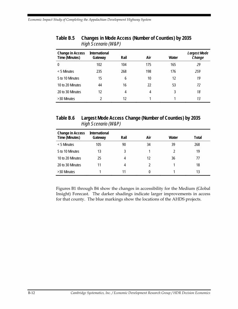
Table B.5 Changes in Mode Access (Number of Counties) by 2035 High Scenario (W&P)


International Gateway Rail Air Water

Largest Mode Change

0 102 104 175 165 29

< 5 Minutes 235 268 198 176 259

5 to 10 Minutes 15 6 10 12 19

10 to 20 Minutes 44 16 22 53 72

20 to 30 Minutes 12 4 4 3 18

>30 Minutes 2 12 1 1 13

Table B.6 Largest Mode Access Change (Number of Counties) by 2035 High Scenario (W&P)


International Gateway Rail Air Water Total

< 5 Minutes 105 90 34 39 268

5 to 10 Minutes 13 3 1 2 19

10 to 20 Minutes 25 4 12 36 77

20 to 30 Minutes 11 4 2 1 18

>30 Minutes 1 11 0 1 13

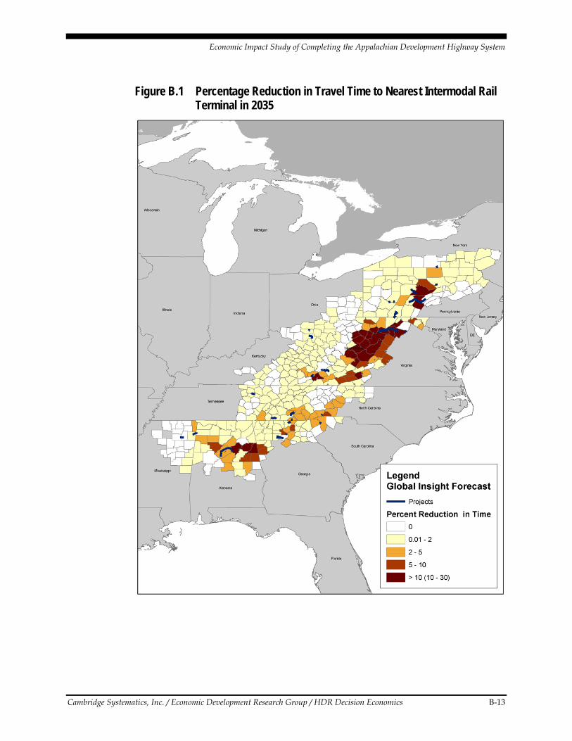
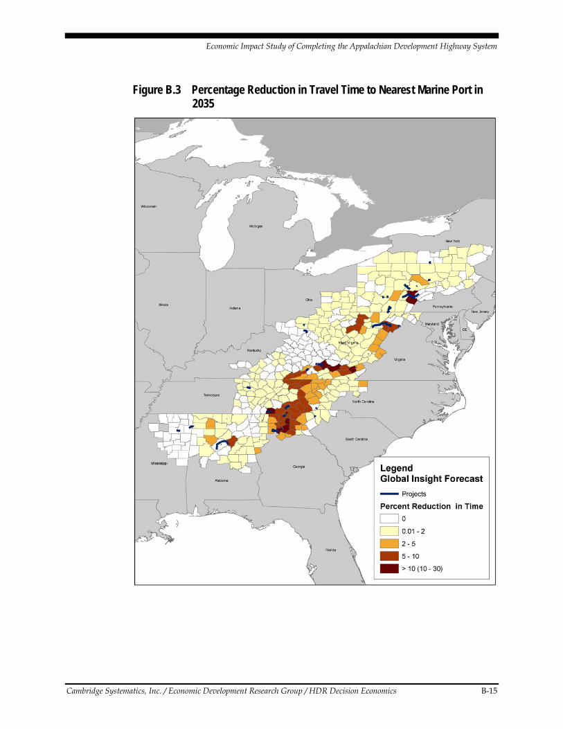
Figures B1 through B4 show the changes in accessibility for the Medium (Global Insight) Forecast. The darker shadings indicate larger improvements in access for that county. The blue markings show the locations of the AHDS projects.



Figure B.1 Percentage Reduction in Travel Time to Nearest Intermodal Rail Terminal in 2035



Figure B.2 Percentage Reduction in Travel Time to Nearest International Gateway in 2035



Figure B.3 Percentage Reduction in Travel Time to Nearest Marine Port in 2035



Figure B.4 Percentage Change in Employment Accessible within a Three-Hour Drive Time (Buyer and Supplier Markets) in 2035



B.3 ESTIMATING THE TIMING AND MAGNITUDE OF ADHS PROJECT IMPACTS An analysis was conducted of the relationship between the timing of highway improvements and the magnitude and timing of subsequent economic growth impacts. This work updates the Twin County Study conducted by EDR Group in 2007.24 The previous study compared growth rates of earnings and income from 391 counties in the ARC to “twin” counties of similar characteristics that were located elsewhere. It tested the impact of the Appalachian Development Highway System on economic growth in the counties of the ARC. For this research, a panel data set was used with each observation consisting of both a county and year – for the purpose of capturing the lagged effect of new lanes on economic growth. While the previous study measured the cumulative effect on growth through 1991 and 2000, this new study estimated the length of time that the opening of a highway (or added lanes) took to affect growth in ARC counties. To capture this impact the variable annual income growth was regressed on new lines miles per area on the current year and up to 10 years before. The hypothe-sis being that a county’s level of distress or metropolitan status could affect the length of time that highway takes to impact growth.

The counties were broken into three groups: metro, non-metro – distressed, and non-metro – non-distressed.25 These categories were created based on whether the county was part of a metropolitan area and its classification of distress level by the ARC. The regression results are illustrated in Figure B.5. They show that distressed counties – after taking longer to react – actually had a larger economic growth impact from non highway development than non-distressed counties.

24 This section is drawn from a working paper by Glen Weisbrod and Tyler Comings,

Economic Development Time Lag from Highway Improvements in Appalachia, using a “twin county” dataset constructed by Theresa Lynch, The Impact of Highway Investments on Economic Growth in the Appalachian Region, 1969-2000: Update and Extension of the Twin County Study, Sources of Regional Growth in Nonmetro Appalachia –Volume 3 Statistical Studies of Spatial Economic Relationships, Economic Development Research Group, MIT Department of Urban Studies and Planning, 2007.

25 The metro group was not broken into two groups because there was no significant difference between distressed and nondistressed counties in metropolitan areas.



Figure B.5 Regression of Annual Income Growth on New Lane Miles Timing of Statistically Significant Impacts Are Shown

Non-Metro, Distressed

05

10152025303540

1 2 3 4 5 6 7 8 9 10 11 12 13

Years Since Highway Completion

Non-Metro, Non-Distressed

05

10152025303540

1 2 3 4 5 6 7 8 9 10 11 12 13


Metro

05

10152025303540

1 2 3 4 5 6 7 8 9 10 11 12 13


Note: Black bars: years with statistically significant values (greater than 90 percent confidence).

Grey bars: fringe years with consistent impact but statistical confidence less than 90 percent.



The estimated impact clearly differs among the different settings. The non-metro – distressed group shows highly significant impact occurring six years after the project. The non-metro – non-distressed has highly significant impact three, four, and five years after project completion. This result is believable and promising as distressed areas should have more potential to grow than other areas. When comparing metro and non-metro categories, it was apparent that nonmetro counties exhibited more of an impact. This result was expected since the ADHS program targets rural areas that lack highway connectivity. Also, highways are concentrated in metro areas; therefore, it seems reasonable that rural areas would be more quickly affected from construction of a new highway. However, it is still a curious result that metro counties are positively affected eight or nine years after project completion.

This analysis, when breaking the counties into groups, provided outcomes that were close to expectations. One implication was that treatment of counties in metropolitan areas should not depend on level of distress. However, it is inter-esting to note that the estimated effect was similar for metropolitan areas to dis-tressed counties not in metropolitan areas, though the latter group received a much larger impact. Treating the nonmetro counties based on their distress level was important. The implication here was that nondistressed counties in rural areas were the fastest to respond to added lanes or new highway construction. Distressed counties that were not in metropolitan areas took longer to respond to the stimulus but had a more intense reaction.

This analysis gave the powerful conclusion that the presence of new highways acted as a catalyst in disadvantaged areas; creating a much needed surge, albeit a delayed one, in economic growth. Therefore, transportation and economic development planners should not anticipate a rapid recovery for these counties when accessibility is improved.

a. travel demand model - appalachian regional · pdf filematrix estimator (odme) procedure to...

Documents