Diplomarbeit

A Tunable Bose-EinsteinCondensate in a Three-dimensional

Optical Lattice Potential

zur Erlangung des akademischen Gradeseines Magisters der Naturwissenschaften

vorgelegt von

Gabriel Rojas Kopeinig

Institut für Experimentalphysikder Naturwissenschaftlichen Fakultät

der Leopold-Franzens-Universität Innsbruck

Juni 2007

Contents

1 Introduction 1

2 Creating a Bose-Einstein Condensate of a Dilute Cesium Gas 52.1 What is a BEC? . . . . . . . . . . . . . . . . . . . . . . . . . . . . . 52.2 Why Cesium? . . . . . . . . . . . . . . . . . . . . . . . . . . . . . . 5

2.2.1 Scattering . . . . . . . . . . . . . . . . . . . . . . . . . . . . 62.2.2 Feshbach Tuning . . . . . . . . . . . . . . . . . . . . . . . . 7

2.3 Producing a Cesium BEC . . . . . . . . . . . . . . . . . . . . . . . 82.3.1 Experimental Setup . . . . . . . . . . . . . . . . . . . . . . . 92.3.2 Experimental Sequence . . . . . . . . . . . . . . . . . . . . . 11

3 Optical Lattice Potentials 153.1 Theory . . . . . . . . . . . . . . . . . . . . . . . . . . . . . . . . . . 15

3.1.1 Dipole Potential . . . . . . . . . . . . . . . . . . . . . . . . . 153.1.2 Periodic dipole potentials . . . . . . . . . . . . . . . . . . . 17

3.2 Experimental Setup . . . . . . . . . . . . . . . . . . . . . . . . . . . 223.2.1 Laser System . . . . . . . . . . . . . . . . . . . . . . . . . . 233.2.2 Light Control . . . . . . . . . . . . . . . . . . . . . . . . . . 243.2.3 Optical Fiber . . . . . . . . . . . . . . . . . . . . . . . . . . 273.2.4 Aiming at the atomic ensemble . . . . . . . . . . . . . . . . 32

4 BEC in an Optical Lattice Potential 394.1 Theoretical Introduction . . . . . . . . . . . . . . . . . . . . . . . . 39

4.1.1 Band structure, Bloch and Wannier functions . . . . . . . . 394.1.2 Bose-Hubbard Model . . . . . . . . . . . . . . . . . . . . . . 434.1.3 Superfluid to Mott Insulator Transition . . . . . . . . . . . . 464.1.4 Loading of a BEC into the Lattice Potential . . . . . . . . . 50

4.2 Testing and Characterizing the Lattice . . . . . . . . . . . . . . . . 554.2.1 Bloch Oscillations . . . . . . . . . . . . . . . . . . . . . . . . 554.2.2 Measuring the Lattice Depth . . . . . . . . . . . . . . . . . . 574.2.3 Lattice-induced Heating . . . . . . . . . . . . . . . . . . . . 62

4.3 Experimental Observations of the Mott Insulator Transition . . . . 684.3.1 Driving the Transition via the Lattice Depth . . . . . . . . . 684.3.2 Driving the Transition via the Scattering Length . . . . . . . 714.3.3 Probing the Excitation Spectrum . . . . . . . . . . . . . . . 74

iii

5 Summary and Outlook 79

iv

1 Introduction

The development of quantum theory in the early half of the last century pavedthe way for major advances in many scientific fields. Although there is still con-troversy on its interpretation, the theory successfully predicts the behavior of themicroscopic world with many of its intriguing phenomena. In an attempt to ob-serve some of the predicted quantum phenomena on a more ’macroscopic’ scale,experimentalist had to find ways on how to reduce or even freeze out thermal ex-citations. The development of laser cooling techniques gave birth to the field ofultracold atomic gases with its first sensational breakthrough in 1995, the creationof Bose-Einstein condensates (BEC) in dilute atomic alkali gases [And95, Dav95].This feat was recognized with the Nobel prize in 2001 for Eric Cornell, WolfgangKetterle and Carl Wieman. Since then, atomic quantum gases have led to newdevelopments and research efforts well beyond traditional atomic, molecular, andoptical physics. Atomic quantum gases have opened up new fields that investigatematter wave lasers and nonlinear matter wave optics, and they have contributedto diverse areas such as condensed matter physics, plasma physics, quantum in-formation and, recently, quantum chemistry. Experimental highlights include theobservation of matter wave interference from independent condensates [And97],the first realization of a matter wave amplifier [Ino99], the excitation of matterwave solitons and vortices [Den00, AS01], and the direct observation of the quan-tum phase transition from a superfluid to a Mott insulator [Gre02a]. For quantumgases with fermionic atoms, the first realization of a degenerate Fermi gas [DeM99]in 1999 was an important milestone.

The success of experiments with ultracold atomic and molecular gases is theresult of an exceptionally high degree of experimental control over most, if not alldegrees of freedom and the ability to prepare very ’clean’ systems in well definedstates. In fact, the control over the quantum degrees of freedom is so high that onecan speak of ’quantum engineering’ of wavefunctions. Internal and external degreesof freedom for atoms in an ultracold gas can be manipulated using magnetic, radio-frequency and optical fields in such a way that coherence can be preserved whilethe system is shielded from the potential perturbations of the environment. It hasnow become routine to control the interaction properties of atoms via magneticand also optically induced Feshbach resonances.

Alkali atoms, such as Li, K, Na, Rb, and Cs, are stil used in the majority ofneutral atom quantum optic experiments. Due to their single valence electron,they have the simplest electronic structure. Cesium was first treated as a primecandidate for condensation [Tie92], but as a result of an unusually high two-bodyloss rate, it is not suited for experiments relying on evaporation in magnetic traps.

1

Therefore an all optical approach is used in the Cs BEC experiments here in Inns-bruck [Web03b, Ryc04]. The great advantage of Cs is that it features a combinationof broad and narrow Feshbach resonances at technically easily accessible magneticfields of a few ten Gauss [Chi00]. This offers great tunability of the interaction andenables the production of pure molecular quantum gases [Her03]. Optical trappingallows the preparation of atomic samples in the lowest internal quantum state,which is immune to inelastic two-body processes, and also permits to fully exploitthe tunability.

An additional and very attractive prospect is the possibility to spatially orderthe atoms. The optical dipole force offers the ability to create periodic latticepotentials for neutral ultracold atoms in one, two or three dimensions. Latticepotentials can serve a wide variety of purposes, like the investigation of phenomenaknown from solid state physics, e.g. the observation of Bloch oscillations [BD96],the suppression of atomic or molecular collisions [Tha06] or the implementation inlaser cooling, e.g. sisyphus cooling.

Loading a BEC into an optical lattice opens the possibility for a great number ofexciting experiments. So far, the experimental highlights with optical lattices in-clude macroscopic quantum interference from atomic tunnel arrays [And98], num-ber squeezing in a 1D lattice [Orz01], quantum phase transition from a superfluidto Mott insulator [Gre02a], collapse and revival of the matter wave field [Gre02b],and repulsively bound pairs in an optical lattice [Win06].

This is the point where the work presented in this diploma thesis ties up to. Byloading a cesium BEC into an optical lattice, we gain experimental access to yetanother key parameter in the investigation of the involved many body dynamics.The capability to tune the atomic interaction properties at will, allows a newgeneration of experiments. The superfluid (SF) to Mott insulator (MI) transitioncan now not only be driven by varying the lattice depth, but also by tuning theatomic interaction strength. This setup also offers the possibility to investigatethe properties of the MI phase as a function of the interaction. Or along thesame lines, the evolution of the MI state while ramping the scattering length tozero or to negative values can be explored. In continuation of the measurementsinvolving Bloch oscillations in a 1D lattice, we can now study the interaction-induced decoherence effects. The combination of the MI state and tunability ofthe atomic interaction strength allows for a controlled association of dimer andpossibly trimer molecules, enabling the measurement of collisional properties fortwo or three atoms a time. It may also serve as a starting point for the realizationof ground state molecules.

The thesis is organized as follows. In chapter 2, a brief summary on how we createa BEC of a dilute Cs gas is given. The particular properties of Cs are introduced,followed by an overview of the experimental setup and of the experimental sequenceas used for the creation of the BEC.

Chapter 3 presents the work that I was mostly involved with during my timeas a diploma student, the implementation of a three-dimensional (3D) optical lat-tice. The theoretical background for the creation of a periodic dipole potential is

2

reviewed in the first part, whereas the technical details are described in the secondpart of chapter 3. A special emphasis is given to the challenges encountered whenworking with relatively high laser powers.

Chapter 4 comprises the presentation of the first experiments using the opticallattice. For better understanding, the theoretical basics describing the single andmany particle physics in a lattice are briefly reviewed. Then, the relevant char-acterization measurements, like the calibration of the lattice depth, are described.The main section of this chapter covers the observation of the quantum phase tran-sition from the superfluid (SF) to the Mott insulating (MI) regime. It reports onour ability to drive the transition by changing the lattice depth, and the promisingindications that we are also able to drive the transition by varying the interactionstrength. The latter is unprecedented so far, and should allow us to examine thedynamics of the SF to MI transition from a different perspective. Last but notleast, the measurement in which we probe the excitation spectrum of the systemin the MI regime is described.

Finally, chapter 5 gives a short summary of the work presented here, and a briefbut exciting outlook on future experiments.

3

2 Creating a Bose-EinsteinCondensate of a Dilute CesiumGas

2.1 What is a BEC?

Bose-Einstein Condensation (BEC) in a gas of particles obeying Bose statisticswas predicted by Einstein in 1924 [Ein25]. His work was based on the ideas ofBose addressing the statistics of photons [Bos24]. The prediction basically stated,that if noninteracting atoms were cooled below a critical temperature, the wholeatomic ensemble would start behaving as one big matter wave, strikingly demon-strating the wave nature of matter. A BEC of a weakly interacting dilute gas ofRubidium atoms was experimentally first demonstrated 71 years after Einstein’spublication [And95]. Such a system provides an unique opportunity for exploringquantum phenomena on a macroscopic scale.

To produce a BEC in a dilute gas, the atoms have to be cooled to extremely lowtemperatures of around 1/1, 000, 000 degree Kelvin above the absolute zero. Forthis a whole range of sophisticated laser cooling techniques have been developed inthe 80’s and 90’s. The realization of a BEC requires a complex experimental setup,including a vacuum chamber, different laser systems for cooling and/or trapping,magnetic fields for trapping and/or manipulation of the internal states, an imagingsystem and a control unit.

2.2 Why Cesium?

• Cesium is an atom of particular interest in physics. It has various importantapplications in fundamental metrology, such as in measurements of the fine-structure constant [Hen00],of a possible electric dipole moment of the elec-tron [Chi01b], parity violation [Bou82], and in measurements of the Earth’sgravitational field [Sna98]. Furthermore, due to its large hyperfine splittingin the ground state, it serves as our primary frequency standard [BIP98]. Bydefinition, one second is 9,192,631,770 periods of the microwave transitionassociated with the hyperfine transitions of the ground state.

• Cesium is very suitable for laser cooling applications. Due to its large mass,the recoil energy is very low. The laser cooling transitions can be readily

5

addressed by low-cost diode laser systems. This and the technical signifi-cance made cesium an interesting and a very promising candidate for Bose-Einstein condensation [Tie92]. However, the particular scattering propertiescomplicate the condensation process substantially, and so the first successfulattempt to condense Cs was carried out here in Innsbruck [Web03b], sevenyears after the first realization of Bose-Einstein condensation of 87Rb atomsin 1995 [And95].

• Cesium is an excellent candidate for experiments with tunable interaction.For Cs in it’s absolute electronic ground state, the scattering length canbe varied via ’Feshbach tuning’. This provides an unique opportunity togain experimental access to a key parameter in the investigation of ultracoldatoms, the interaction energy.

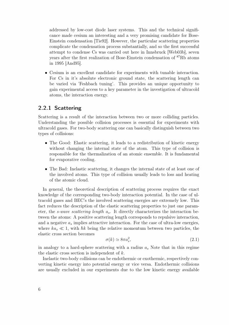
2.2.1 Scattering

Scattering is a result of the interaction between two or more colliding particles.Understanding the possible collision processes is essential for experiments withultracold gases. For two-body scattering one can basically distinguish between twotypes of collisions:

• The Good: Elastic scattering, it leads to a redistribution of kinetic energywithout changing the internal state of the atom. This type of collision isresponsible for the thermalization of an atomic ensemble. It is fundamentalfor evaporative cooling.

• The Bad: Inelastic scattering, it changes the internal state of at least one ofthe involved atoms. This type of collision usually leads to loss and heatingof the atomic cloud.

In general, the theoretical description of scattering process requires the exactknowledge of the corresponding two-body interaction potential. In the case of ul-tracold gases and BEC’s the involved scattering energies are extremely low. Thisfact reduces the description of the elastic scattering properties to just one param-eter, the s-wave scattering length as. It directly characterizes the interaction be-tween the atoms: A positive scattering length corresponds to repulsive interaction,and a negative as implies attractive interaction. For the case of ultra-low energies,where kas � 1, with hk being the relative momentum between two particles, theelastic cross section becomes

σ(k) ' 8πa2s, (2.1)

in analogy to a hard-sphere scattering with a radius as Note that in this regimethe elastic cross section is independent of k.

Inelastic two-body collisions can be endothermic or exothermic, respectively con-verting kinetic energy into potential energy or vice versa. Endothermic collisionsare usually excluded in our experiments due to the low kinetic energy available

6

at µK-temperatures. An exothermic collision mainly occurs as a result of a spin-exchange process (with the total mF conserved) or, in particular for Cs, due to themagnetic dipolar interaction (in a spin relaxation process with the total mF notbeing conserved). These type of collisions release energy into the sample and causeheating and/or loss from the trap. For this reason, we work with Cs atoms in theabsolute electronic ground state (F = 3,mF = 3), where all inelastic two-bodycollisions are fully suppressed. For a detailed description of the basic principles Irefer the reader to one of many review articles on this subject, e.g. Ref. [Dal99].

In the absence of inelastic two-body collisions the dominant loss mechanism isdue to three-body recombination [Web03c]. It is the process of two atoms forminga dimer molecule in a collision with a third atom. The third atom needs to bepresent to satisfy momentum and energy conservation. In the context of atomtrapping, three-body recombination primarily leads to particle loss, but it alsoleads to heating of the sample. Luckily, Bose-Einstein condensation occurs ina regime where densities are sufficiently low so that the probability for a three-body recombination event is rather small. Condensates can have lifetimes of 30 sand beyond, quite often limited by collisions with the background gas and not byinternal processes. For Cs, the three-body loss rate coefficient L3 is on the order of1028 cm6/s [Kra06]. The atom density should then be well below 1014 atoms/cm3

to allow for sufficiently long lifetimes for the atomic sample.

2.2.2 Feshbach Tuning

For inelastic collisions the incident and outgoing scattering wave functions experi-ence different interaction potentials. These potentials are also called entrance andoutgoing channels. If the energy of an outgoing channel is lower than the totalenergy of the incident channel, inelastic exothermic collisions to that channel arepossible. This channel is then called open channel. If the energy of the outgoingchannel is higher, inelastic scattering to this channel is not possible. It is thereforecalled a closed channel. Since the two colliding atoms in (F = 3,mF = 3) havethe lowest internal energy, there are no open channels available. However, closedchannels can also alter the (elastic) scattering parameters dramatically.

Usually, as illustrated in Fig. 2.1, it is sufficient to consider two channels, anentrance channel and a closed channel with a single molecular bound state. AFeshbach resonance [Ino98] occurs when the state of two free atoms in the entrancechannel is allowed to couple to the closed channel with a molecular bound state.For this, the bound state has to be brought into degeneracy with the entrancechannel, usually by means of an external magnetic field and the Zeeman effect,making use of the fact that different channels have different magnetic moments.As the energy level of the molecular state approaches that of the entrance channel,the scattering length as diverges. If the molecular state is close to but below(above) the energy of the incident state, the scattering length is large and positive(negative). The coupling between entrance channel and closed channel is the resultof strong electronic interactions such as the exchange interaction and weaker dipole-

7

dipole and spin-orbit interactions. The former interaction preserves orbital angularmomentum and leads to strong s-wave Feshbach resonances, the latter leads toweaker higher-order d-wave, g-wave, etc. Feshbach resonances [Chi04].

Figure 2.1: The Feshbach resonance scenario: (left) By applying an external mag-netic field, the scattering state of two free atoms in the entrance channelcan be brought into energetic degeneracy with a molecular state belong-ing to the closed channel. (right) In the vicinity of the state crossing(bottom) the scattering length a shows a dispersive divergence (top).

The width ∆B of a Feshbach resonance is determined by the magnetic moment ofthe bound state and the coupling strength between the two states. If the scatteringlength far from any resonance is abg then the scattering length around the resonanceposition Bres can be calculated by

a(B) = abg

(1− ∆B

B −Bres

). (2.2)

Figure 2.2 shows several Feshbach resonances the (F = 3,mF = 3) × (F =3,mF = 3) scattering channel, where as is plotted against the magnetic field B.

Feshbach resonances offer the possibility to tune the scattering length and thusthe interatomic interaction. This is often referred to as Feshbach tuning. Feshbachresonances can also be used to create molecules [Her03, Reg03]. A detailed discus-sion on Feshbach resonances in general and their use as a tool for the production ofcold molecules is found in a review by T. Köhler [Köh06]. A discussion on Feshbachresonances particularly for Cs can be found in [Chi01a].

2.3 Producing a Cesium BEC

The realization of a Cs BEC requires an involved experimental setup, including avacuum chamber, different laser systems for cooling and trapping, magnetic fieldsfor the application of magnetic forces and for a control of the interaction strength

8

Figure 2.2: Scattering length in units of Bohr’s radius a0 as a function of the mag-netic field for the electronic ground state of cesium, F = 3,mF = 3.There is a Feshbach resonance at 48.0G due to coupling to a d-wavemolecular state. Several very narrow resonances at 11.0, 14.4, 15.0, 19.9and 53.5G are visible, which result from coupling to g-wave molecularstates. The quantum numbers characterizing the molecular states areindicated as (l, f,mf ). This plot is taken from [Chi01a].

via Feshbach tuning, and an imaging system. A control system switches and adjuststhese devices on a micro-second timescale to produce an elaborate experimentalsequence with a typical duration of about 10 seconds. This chapter gives a quickoverview on our experimental setup and sequence as used for the creation of aCs BEC. For an further details the reader is referred to the diploma theses of mypredecessors [Unt05, Fli06].

2.3.1 Experimental Setup

The setup used for this work is the third and newest in a series of cesium BECexperiments performed here in Innsbruck. The layout is basically based on thefirst generation setup [Web03a, Web03b], with one essential improvement: Theexperimental chamber made of steel has been replaced by a glass cell, offering,among other things, a greater optical access for the implementation of a three-dimensional optical lattice. Another main advantage is that it also allows forfaster switching of the magnetic fields.

Vacuum Chamber

Experiments with ultracold gases require that the collision rate with the back-ground gas has to be kept as low as possible. Thus the experiments are performed

9

within an ultrahigh-vacuum (UHV) chamber, which is comprised of various ele-ments (Fig. 2.3). It can be roughly divided into two sections: The oven section,which consists of the cesium oven, a series of vacuum pumps and a small cellallowing optical access. The main section includes the Zeeman slower, the ex-perimental glass cell and more vacuum pumps. They are joint via a differentialpump section to accommodate the pressure difference of more than 7 orders ofmagnitude(∼ 3 · 10−4 mbar in the oven and < 10−11 mbar in the experimentalchamber).

Figure 2.3: Schematic drawing of the vacuum chamber. The apparatus has a lengthof 180 cm and can be divided into an oven section and a main section.Magnetic coils to generate the gradient and bias magnetic fields sur-round the glass cell. The compensation coils are not shown.

Laser Systems

Laser cooling of Cs requires laser light at a wavelength of 852 nm and a line widthof <100 kHz. It is generated by two home-built grating-stabilized diode lasersin Littrow configuration serving as so-called master lasers, and three home-builtinjection-locked diode lasers, serving a slaves. They provide the light for the follow-ing applications: Zeeman slowing, magneto optical trap (MOT) operation, Raman-sideband cooling, and for the imaging system.

The far detuned laser light for trapping the atoms is provided by a commercialhigh power Ytterbium fiber laser operating at 1070 nm delivering up to 100W oflaser power (model number YLR-100LP, IPG).

10

Magnetic coils

The magnitude and direction of the magnetic field plays a key role during the entireexperimental sequence. Therefore a total of 16 coils have been installed, formingthe following magnetic coil systems:

• Bias and gradient field coils: They can generate bias fields of up to 200 Gand field gradients of up to 70 G/cm along the vertical direction. The preciseand fast control of these fields is substantial for various applications, e.g. forthe MOT, for Feshbach tuning, for atom levitation, etc.

• Compensation coils: These coils enclose the whole main section of the vacuumchamber and are mostly responsible for the compensation of various strayfields, like the earth’s magnetic field, or the fields produced by the ion getterpumps. They also control the field during Raman sideband cooling.

• Zeeman slower coils: In combination with the Zeeman laser beam, these coilseffectively decelerate the atoms from about 260m/s to almost zero.

Imaging system

The atom cloud is imaged using the standard absorption imaging method [Ket99].A resonant laser beam is shone onto the cloud, producing a shadow image onthe chip of a CCD-camera. This image can be directly translated to a (projected)atom density. The pictures are immediately analyzed to give the relevant data, e.g.atom number, atom cloud position and width, etc. The processing and analyzingof the images is performed with a MATLAB-program. Ensemble temperatures aredetermined by the time-of-flight (TOF) technique.

Control System

The experimental sequence can be controlled by a computer program written inVisual C++. It was adapted for our setup from the original version developed by F.Schreck [Sch]. The software communicates with the different experimental devicesvia a computer card (NI6533, National Instruments) and a home-built bus system.The card outputs the digital data onto the bus with 200 kHz, which allows a timingresolution of 5µs. Currently, we use about 20 analog and 50 digital outputs and6 direct digital synthesis devices (DDS) connected to the bus system, addressingthe numerous experimental devices.

2.3.2 Experimental Sequence

The following experimental steps (see also Fig. 2.5 are performed to create a Bose-Einstein condensate of up to 200,000 atoms:

11

• Zeeman slowing: The atomic beam coming from the Cs oven with a tem-perature of about 380K is decelerated from about 260m/s to a few m/s in68 cm [Met99]. At this point the atoms are slow enough to be trapped in thefollowing step.

• Magneto-optical trap: Within 2 s around 2 · 108 atoms are captured in themagneto-optical trap (MOT). For the last 25 ms the detuning is decreasedfrom -10 to -70MHz in order to spatially compress the atom cloud to adiameter of ∼ 600µm [Met99]. After this step, the temperature has droppedto about 45µK.

• Raman sideband cooling: After the compressed MOT, the lasers for Ramansideband cooling (RSC) are turned on. This dark state cooling scheme notonly decreases the temperature of the atoms, but also polarizes the atomsinto their electronic ground state (F = 3,mF = 3) [Dav94]. After only 6.5msthe ensemble has reached a temperature of ∼ 700nK at a phase space densityof ρ ∼ 10−3. At this point the total atom number has decreased to about7 · 107 [Fli06].

• Reservoir trapping: The reservoir trap can be viewed as an intermediatestep for loading the atoms into the so-called dimple trap [SK98, Kra04]. Itconsists of two crossed red-detuned high power laser beams at 1070 nm witha relatively large beam diameter of ∼ 0.5mm. Since the reservoir trap andthe subsequent trapping schemes are too weak to hold the atoms againstgravity, it is necessary to switch on the magnetic levitation fields at thisstage. Imperfect mode matching heats the atoms during the loading of thereservoir trap to a couple of µK. Therefore the trap is left on for 1 s at ascattering length ∼ 1500 a0. During this time the hottest atoms evaporateout of the trap. After this process we have about 1 · 107 atoms at ∼ 1µKwith a phase space density of ρ ∼ 5 · 10−3.

• Dimple trapping: To further increase the phase space density toward thepoint of condensation, we use the dimple-trick [SK98, Kra04]. Therefore twoadditional tightly focused laser beams are adiabatically ramped up (Fig. 2.4),creating a dimple in the existing potential of the reservoir trap. This increasesthe density in the tight dimple trap without an increase in temperature as theatoms in the reservoir trap act as a temperature bath. During this processthe scattering length is reduced to ∼ 470 a0 to avoid three-body losses. Afterthe loading of the dimple (1 s) one of the reservoir beams is switched off. Thisway the atom reservoir is drained, leaving only the compressed atoms in thedimple. With the scattering length set to ∼ 330 a0 (low tree-body collisionrate) we wait for 300 ms for the ensemble to thermalize. This procedure givesnearly 1.7 · 106 atoms with a similar temperature than after RSC, but with aphase space density ρ ∼ 10−1 that is about two orders of magnitude larger.

12

• Forced evaporation: During this final process the depth of the dimple po-tential is successively reduced. In 3-4 steps the light power of the dimplebeams is slowly (∼ 5 s) ramped down, allowing the hottest atoms to escape.This effectively lowers the temperature of the remaining ensemble. At thepoint where the ensemble has reached the critical temperature Tc ' 20 nK,condensation sets in, and a macroscopic population of the atoms populatethe quantum mechanical ground state. This is the actual starting point forthe experiments presented in this work.

We usually work with a condensate of about 1.5 · 105 atoms. At the end ofa typical evaporation procedure the trap frequencies of the dimple trap areνx = 20 Hz, νy = 18 Hz, and νz = 27 Hz. The BEC fraction is then around80% and the Thomas-Fermi radius rTF ' 13µm (with a scattering length as

of 210 a0).

Figure 2.4: Illustration of the dipole trapping stages: In the reservoir trap theatoms are trapped by two crossed high power laser beams with rela-tively large beam diameters. To increase the phase space density, twoadditional tightly focused beams are superimposed, effectively increas-ing the density without raising the temperature, since the atoms in thereservoir act as a temperature bath. Then the atom reservoir is drainedby switching off one of the reservoir beams. After some thermalizationtime, the dimple potential is slowly ramped down, allowing hottestatoms to escape, effectively lowering the temperature of the remainingensemble.

13

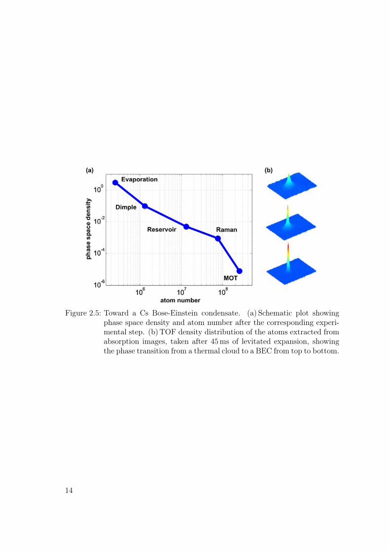
Figure 2.5: Toward a Cs Bose-Einstein condensate. (a) Schematic plot showingphase space density and atom number after the corresponding experi-mental step. (b)TOF density distribution of the atoms extracted fromabsorption images, taken after 45ms of levitated expansion, showingthe phase transition from a thermal cloud to a BEC from top to bottom.

14

3 Optical Lattice Potentials

An accessible way of manipulating the external states (e.g., position and velocity)of a neutral atom is through its interaction with an electromagnetic wave. Theinteraction can be of a dissipative and/or conservative nature. Both are fundamen-tal for our experiments with neutral atoms. Dissipation of energy arises throughthe absorption of a photon followed by a spontaneous reemission of a photon witha slightly different wavelength. The resulting momentum transfer forms part ofthe underlying principles of all laser cooling schemes. On the other hand, the in-teraction of the light-field-induced dipole moment of the atom with the light fielditself, can be used to create a conservative potential for the atoms by the way ofthe so-called ac Stark shift. This chapter describes how we use this fact to createa three-dimensional lattice potential.

3.1 Theory

3.1.1 Dipole Potential

In this section we will recapitulate the results for the dipole potential due to theconservative part of the interaction between the light field and light-field-induceddipole moment. We will also introduce the basic equations for the photon scatteringrate and show that the residual photon scattering can be neglected for the case ofa far-detuned optical trap. For a more detailed discussion please refer to one ofthe more comprehensive review articles, e.g. [Gri00].

Two-level atoms in a near-resonant trap

The following expressions for dipole potential Vdip and scattering rate Γsc can beused for optical traps with a laser frequency that is relatively close to an atomicresonance. These traps can be considered far-detuned in the sense that the de-tuning ∆ is large with respect to the atomic line width ∆ � Γ. However, theabsolute value of the detuning has to be much smaller than the resonance fre-quency |∆| � ω0, since the rotating wave approximation (RWA) has been appliedto obtain

Vdip(r) = −3πc2

2ω30

Γ

∆I(r) and (3.1)

Γsc(r) =3πc2

2hω30

Γ2

∆2I(r). (3.2)

15

Here, c is the speed of light, ∆ = ω − ω0 is the detuning of the laser frequency ωfrom the atomic resonance frequency ω0, Γ is the linewidth of the atomic transitioncorresponding to the spontaneous decay rate of the excited state, and I(r) is thespatial laser light intensity distribution.

For our setup with a 1064 nm light source, the requirement for the rotating waveapproximation |∆| � ω0 is not really fulfilled, so that errors in the order of 10%and 50% respectively would be made (see Tab 3.1). Nevertheless, Eq. (3.1) and(3.2) help us to stress two important points:

• Sign of detuning: Atoms that are in the light field of a red detuned (∆ < 0)laser beam will be attracted to positions of maximum intensity, whereasatoms in a blue detuned light field (∆ > 0) will be drawn to positions ofminimum light intensity. Therefore we can use the dipole-force to orderatoms in space by applying laser light with spatially modulated intensity.

• Scaling with intensity and detuning: Both the dipole potential and the scat-tering rate, scale linearly with the light intensity, but the potential is propor-tional to 1/∆, whereas the scattering rate exhibits a 1/∆2 dependence. Thatmeans that one can create deep potentials with low scattering rates by usinglaser light with high intensity and large detuning from atomic resonance.

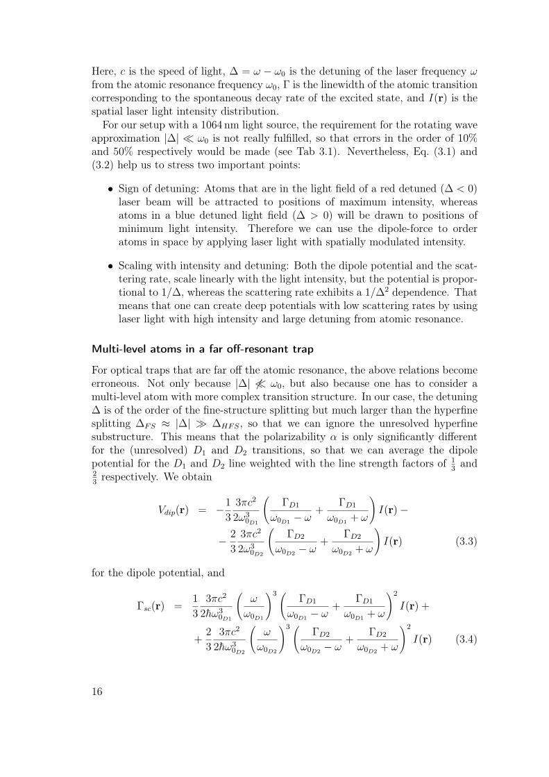
Multi-level atoms in a far off-resonant trap

For optical traps that are far off the atomic resonance, the above relations becomeerroneous. Not only because |∆| 6� ω0, but also because one has to consider amulti-level atom with more complex transition structure. In our case, the detuning∆ is of the order of the fine-structure splitting but much larger than the hyperfinesplitting ∆FS ≈ |∆| � ∆HFS, so that we can ignore the unresolved hyperfinesubstructure. This means that the polarizability α is only significantly differentfor the (unresolved) D1 and D2 transitions, so that we can average the dipolepotential for the D1 and D2 line weighted with the line strength factors of 1

3and

23

respectively. We obtain

Vdip(r) = −1

3

3πc2

2ω30D1

(ΓD1

ω0D1− ω

+ΓD1

ω0D1+ ω

)I(r)−

− 2

3

3πc2

2ω30D2

(ΓD2

ω0D2− ω

+ΓD2

ω0D2+ ω

)I(r) (3.3)

for the dipole potential, and

Γsc(r) =1

3

3πc2

2hω30D1

(ω

ω0D1

)3 (ΓD1

ω0D1− ω

+ΓD1

ω0D1+ ω

)2

I(r) +

+2

3

3πc2

2hω30D2

(ω

ω0D2

)3 (ΓD2

ω0D2− ω

+ΓD2

ω0D2+ ω

)2

I(r) (3.4)

16

for the scattering rate.At this point it should be noted that these results only account for E fields

with linear polarization and that for circular polarization the line strength factorsdepend on the magnetic quantum number mJ , and on the sign of the rotation(σ+ or σ−). See review of dressed state approach [Gri00]. In other words, the acStark shift depends not only on the intensity, but also on the state of polarization(π, σ+, σ−) (see e.g. sisyphus effect [Gui99]).

Typical Values

To conclude this chapter some values for realistic beam parameters are given inTab. 3.1. It is always convenient to specify the potential depth in energy units ofpossible perturbations. When working with ultra cold gases in dipole potentialsa possible perturbation is a photon scattering process. Therefore units of recoilenergies

Er = h2k2/2m, (3.5)

where m is the atom mass, and k = 2π/λ the wave vector of the laser light, areused throughout this work.For a Cesium atom and a laser wavelength of 1064nm it can be converted asfollows:1 Er = 8.78 · 10−31 J = 64 nK = 1325 Hz

853 nm 1064 nm 10000 nmno RWA with RWA no RWA with RWA no RWA with RWA

Vdip 8450 Er -0.01% 10.4 Er -9.3% 307 Er -46%840µK 660 nK 220 nK

Γsc 2 · 104 s−1 +0.02% 4 · 10−3 s−1 +51% 5 · 10−7 s−1 +400%

Table 3.1: Potential depth and photon scattering rate for a Cs-atom in a Gaussianlaser beam with a power of 1 W, a waist of 500µm and different wave-lengths. The values are calculated without rotating wave approximation(RWA). The respective errors of the RWA are also given. Note that theunit Er is not very suitable for comparing potential depths for differentwavelengths as it is wavelength dependent itself.

3.1.2 Periodic dipole potentials

As we have seen in the previous section, one can use laser beams to trap atoms inpositions of maximum light intensity. By creating a spatially intensity-modulatedlaser light field, e.g. a standing wave, one can produce periodic lattice potentialsin 1, 2 or 3 dimensions.

17

1D lattice potentials

The simplest realization of a spatially modulated light field is to let two counter-propagating laser beams interfere. If they have identical wavelengths λ and parallelpolarizations, the result is a standing wave with a periodicity in z-direction of λ/2,with λ being the laser wave length. The E field takes the form

E = 2E00 cos kze−iωt, (3.6)

where E00 is the amplitude of the electric field, and k = 2π/λ and ω are thewave vector and the frequency of the laser beam with propagation direction z. Invacuum, k and ω relate via k = ω/c. If we also consider the fact that the laserbeams have a Gaussian intensity-profile of the form

I(r) = I0e− 2r2

w2 , (3.7)

the potential can be written as

V (r, z) = V01De−

2r2

w2 cos2 kz. (3.8)

Here r is the radial distance from the beam center, I0 = 2Pπw2 is the peak-intensity,

w = w(z) = w0

√(1 + (z/zR)2) is the 1

e2 -radius (waist) of the beam, zR = πw2/λ

is the Rayleigh length and V01D= 4Vdip(r = 0) is the maximum potential depth

in the 1D lattice. The potential Vdip(r = 0) is calculated from Eq. (3.3) for I0.Because of the |E|2-dependence we obtain a four times deeper dipole potential fortwo interfering beams, than for a single beam. As we are only interested in spatial

Figure 3.1: Illustration of a dipole potential for a Gaussian laser beam (a) and an1D lattice potential formed by two counter-propagating Gaussian laserbeams (b).

regions of the order of the waist w0 � zR, we will neglect the z-dependence of thewaist in the following discussions.

2D lattice potentials

The standard way to create a periodic lattice in two dimensions is to superim-pose two pairs of counter-propagating beams in an orthogonal configuration. (See

18

Fig. 3.2 for the effect of different angles between orientation and polarizations ofthe two beam-pairs.) Assuming identical amplitudes for the four beams, the E fieldcan be expressed as

E = E00(e1ei(kx−ωt+ϕx) + e1e

i(−kx−ωt+ϕx) + e2ei(ky−ωt+ϕy) + e2e

i(−ky−ωt+ϕy)

= 2E00(e1 cos kx+ e2 cos kyei(ϕy−ϕx))eiωt, (3.9)

with e1 and e2 being the polarization vectors of the beam pairs in x- and y-direction, respectively. Since we are only interested in length scale on the order ofthe atomic cloud we will neglect the Gaussian beam profile. For equal frequenciesthe potential takes on the form:

V (x, y) = V01D(cos2 kx+ cos2 ky + 2e1 · e2 cos ∆ϕ cos kx cos ky) (3.10)

We can see that in general the result still depends upon the phase difference be-tween the beam-pairs ∆ϕ = ϕy − ϕx, making it sensitive to phase fluctuations.To avoid this undesired effect (which could lead to heating of the atoms) one canchoose orthogonal polarizations between the standing waves so that e1 ·e2 vanishes.As one can see in Fig. 3.2 the effective potential depth (being the potential barrierfrom one lattice site to the nearest) is four times smaller than for parallel polariza-tion vectors in this case, but it makes a experimentally involved implementationof a phase-stabilization unnecessary (see Fig. 3.3). Instead, or additionally to theorthogonal polarizations, one can introduce a slight frequency difference (MHz)between the two laser beams. In this case the potential varies its depth and formon a µs time scale, which is much to fast for the atom to follow. The time-averagedpotential ’seen’ by the atoms is then identical to a potential produced with twostanding waves with orthogonal polarizations.

3D lattice potentials

In general a 3D optical lattice can be realized in many different ways. In [Pet94] itis shown that the Bravais lattice is determined from the propagation directions ofthe laser beams while, the basis is associated with the polarizations of the incidentwaves. In the ’standard tetrahedron’ configuration one could generate a threedimensional lattice with only four beams, but because we want to accommodatea 1D, 2D and 3D lattice with the same experimental setup, we use six beams toform three standing waves that are mutually orthogonal. Again, to be insensitiveto phase fluctuations, one can set the polarizations between the standing wavesto be mutually orthogonal, or one can offset the frequencies between the differentstanding waves by a few MHz by means of acousto-optical modulators. Bothmethods create a simple cubic lattice potential for the atoms with a periodicityof λ/2 (see Fig. 3.4). The resulting lattice potential is just the sum of threeindependent 1D lattice potentials (see Eq. 3.8), so that we can write

V (x, y, z) = V01D,xe−2 y2+z2

w2x cos2 kx+ V01D,y

e−2x2+z2

w2y cos2 ky + V01D,z

e−2x2+y2

w2z cos2 kz.

(3.11)

19

Figure 3.2: 2D lattice potentials formed by two pairs of counterpropagating beamsfor different configurations. Here k1 = −k2, k3 = −k4, e1 = e2 ande3 = e4 are the wave- and polarization-vectors of the four plane waves.

20

Figure 3.3: 2D lattice potentials for two orthogonal standing waves for variousphase differences ∆ϕ with a) parallel polarizations and b) orthogonalpolarizations

Figure 3.4: Schematic illustration of the equipotential surface of a simple cubiclattice as formed by superimposing three orthogonal standing waves.

21

Here V01D,x, V01D,y

and V01D,zare the maximum potential depths for 1D lattices

formed by counter-propagating laser beam pairs in x, y and z direction respectively.Remember that, e.g. V01D,x

= 4Vdipx is the potential barrier between lattice sites inx direction, generated by two interfering beams each with intensity I0x , with Vdipx

being the potential depth created by one single beam in x direction with intensityI0x (see Eq. [3.3]).

Typical Values

The following table 3.2 is intended as a quick reference for the expected latticedepth for a laser wavelength of 1064nm. Note that, if the standing waves havemutually orthogonal polarizations or are mutually detuned, then the potentialbarrier to the nearest neighbors in a 2D or 3D lattice is the same as in a 1Dlattice. Whereas the potential barrier to the next neighbor in diagonal direction(in the plane spanned by two standing waves, e.g., in x and y direction) is thenV01D,x

+ V01D,y, and in the direction of the space-diagonal (for a 3D lattice only)

the potential barrier is V01D,x+ V01D,y

+ V01D,z. Throughout the rest of this work,

if not otherwise stated, the term lattice depth refers to the (physically significant)potential barrier between nearest neighbor sites V01D

(at the center of the Gaussianbeams) rather than to the actual potential depth. Obviously, this lattice depth canbe different for each lattice axis.

Laser Power P Beam Waist w Lattice Depth V01D

1 W 500µm 41.6 Er

P in W w in µm 41.6P(

500w

)2in Er

Table 3.2: Lattice depth calculated for a laser wavelength of 1064nm for a one-dimensional lattice, corresponding to the potential barrier between near-est neighbors for a multi-dimensional lattice with mutual orthogonalpolarizations or mutual detuning.

3.2 Experimental Setup

The general idea for the experimental implementation of a 1D, 2D or 3D opticallattice is very simple: One takes 1, 2 or 3 laser beams (from a single or differentsources) and creates a standing wave for each desired dimension by just retro-reflecting each beam on a mirror as shown in Fig. 3.5.

Figure 3.5: A simplified picture on how to create a one-dimensional optical lattice

22

The actual realization is a bit more involved: One needs to take into account theusual components for the ability to control and adjust the laser light, e.g. acousto-optic modulators (AOM’s), lenses, adjustable mirrors and so on. Because thereis only a limited amount of space around the experimental chamber, we built thelight source and necessary hardware to split and control the laser light a couple ofmeters away from the glass cell (see Fig. 3.6). For increased stability in terms ofbeam pointing and for better beam-profile quality, the laser light is guided to theexperimental chamber using optical fibers. We chose to create two standing wavesby retro-reflection, and the third by interfering two counter-propagating beams.This allows us to accelerate the lattice along one direction, a feature that will beused in future experiments.

Figure 3.6: Schematical drawing of the experimental setup divided into its fourmain parts: laser system, light control, optical fibers, and aiming atthe atomic ensemble.

The following sections describe the technical aspects of the experimental setupin more detail. Table 3.3 shows summarizes of the requirements that had to betaken into account.

Requirements Dependence Measureslattice depth V0 > 30 Er ∝ P

(1

∆w2

)high power P ∼ 1 W

beam

scattering rate Γsc < 10−1 s−1 ∝ 1∆2

(Pw2

)far detuned λ =1064 nm

uniform lat. depth ∆V0

V0< 5% ∝

(1

w2

)large b. waist w ∼ 500µm

Table 3.3: Table showing the requirements on the experimental setup and theirdependence from the laser beam power P , the detuning ∆, and the beamwaist w. The chosen and the corresponding values are also shown.

3.2.1 Laser System

A uniform lattice depth of up to 50 ER would be desirable. For beam diametersof about 1 mm one thus needs around 1.25W of optical laser power per beam.

23

Having four beams (two retro-reflected and two counter-propagating) and with atotal transmission efficiency of the optical components of roughly 50%, we needa laser output of >10 W. For this purpose the light of a commercial narrow bandNd:YAG laser at 1064 nm (model name Mephisto, Innolight) is amplified by ahome-built Ytterbium-doped large-mode-area fiber [AL03], providing up to 15 Wof narrow-band light. The output beam is collimated to a waist of about 900µm.With a line width of about 1 kHz, this light source exceeds the required coherencelength of a couple of meters by many orders of magnitude. Further details will beavailable in [Hal].

3.2.2 Light Control

Experiments with optical lattices require good control over the applied laser light.One needs to be able to ramp and switch the light intensity on a µs-timescalewhich can easily be done with acousto-optic modulators (AOM’s). Because theuse of optical fibers always introduce intensity fluctuations (see next chapter), anactive stabilization of the light intensity is essential.

Figure 3.7: Schematical drawing of the optical setup used to control the laser light.

General Setup

The collimated beam from the fiber amplifier is split into four beams using thin-filmpolarizer cubes (model number G335723000, Linos). The ratio of the intensities ofthe divided beams can arbitrarily be chosen by placing a λ/2-waveplate in frontof each polarizer cube (see Fig. 3.7). For an efficient AOM operation a 1/e2-beam

24

waist of about 500µm is needed. Therefore the waist is reduced by means of atelescope. The diffracted beam (the 1st or −1st order) is then expanded with a pairof lenses to obtain the necessary mode-matching for a efficient air-fiber coupling.This is critical, since the damage threshold of the fiber decreases with the couplingefficiency (see section 3.2.3). A λ/2-waveplate is placed in front of the fiber-couplerto match the polarization axis with the fast axis of the polarization-maintainingfiber.

Mirrors

We use standard dielectric mirrors with high-reflectivity coatings at 1064 nm. Theyhave the highest reflectivity for light with the linear polarization direction perpen-dicular to the plane of incidence (s-polarized), and they are designed to be usedat an angle of 45◦ to the beam. These facts were taken into account wheneverpossible. One must also consider that the reflected light experiences a differentphase-jump for its s- and p-component. For reasons that are described later, itis important to maintain the linear polarization of the light. Therefore one mustexclusively use the mirrors for s- or p-polarized light.

AOM / rf-driver / PI-control

An AOM uses the acousto-optic effect to diffract the beam and to shift the fre-quency of light using sound waves in a crystalline material. These sound waves aregenerated by a piezo that needs to be driven with a radio-frequency (rf) signal.The AOM’s used in our setup (model number 3110-197, Crystal Technology) re-quire power of up to 2.5 W at a center frequency of 110 MHz. Their bandwidth is15 MHz. The rf-signal is generated by a direct digital synthesis device (DDS, modelnumber AD9852, Analog Devices) [Mey], which can be directly addressed by theexperiment control program to set frequency and amplitude to the desired values.This signal is amplified in two steps to a maximum power of 34 dBm. The home-built amplifier circuit includes a variable attenuator, which is used to stabilize thelight intensity after the optical fiber to a desired value with a proportional-integral(PI) control circuit. (See Appendix A for the electronic circuits.) The transmittedlight power is deduced via a photo-diode (PD) that is place behind the first mirrorafter the optical fiber (see Fig. 3.13 and Fig. 3.14). Because the mirrors have areflectivity of about 99.5% and because we work with intensities of the order of1 W, the ’leaking’ light is sufficient to be detected by a regular PD. The desiredlight power can be entered in the experiment-control-program and is passed onto the PI-control through a digital analog converter (DAC). An useful feature ofthe PI-control is, that the stabilization can be switched on and off (sample andhold mode) during the experimental sequence. When the stabilization is on, theramping speed of the lattice depth is limited by the PI-control (∼ 500µs). For mea-surements where faster switching is required (see e.g. sec. 4.2.2), the stabilizationis turned off during ramping.

25

Thermal effects

A serious problem are the thermal effects of the AOM when it is switched onabruptly. This effect is especially pronounced when the AOM is cold. It is due tothe heat generated by the rf-signal, causing thermal dilation of the AOM crystal.The effect manifests itself, among other things, in a spatial drift of the diffractedbeam on timescale on the order of a couple of seconds. As a consequence, the fibercoupling efficiency decreases, which can, if one tries to switch high-power laserlight, permanently damage the optical fiber. See section 3.2.3 for a more detaileddiscussion of the damage threshold of the fiber. This beam pointing error canbe reduced if the AOM is placed in the focus of two lenses forming a telescope,resulting in a fairly small beam waist at the position of the AOM. For a wavelengthof 1064 nm, the AOM’s need a relatively large beam waist (> 500µm) to obtaindecent diffraction efficiencies. Therefore we chose a trade-off where we positionedthe AOM in the collimated beam with a waist of 400 − 450µm, and tried tominimize the optical distance between AOM and fiber-coupler.

Damage threshold of optical components

As we are working with laser beams with up to 15W of power, one has to considerthe manufacturer-specified damage threshold of the optical components used in thesetup. Table 3.4 summarizes the collected data on damage threshold for severalcomponents.

Component Specified DT Applied peak-int. CommentCube(PBS) 2 kW/cm2 ∼ 1.2kW/cm2 thin film polarizers, Linosλ/2-waveplate 2 MW/cm2 ∼ 1.2kW/cm2 multi-order, Thorlabs1

unknown ∼ 1.2kW/cm2 multi-order WP, CasixLenses unknown ∼ 2kW/cm2 BK7 with AR-coating, CasixAOM 10 MW/cm2 ∼ 2kW/cm2 Crystal Technology

Aspheric lens 100 W/cm2 ∼ 400W/cm2 for fiber coupler, Thorlabs2

Table 3.4: Specified damage threshold (DT) and applied laser intensities for theoptical components used in our setup. (1)Reflections from other opticalcomponents melted the glue in the mounting. Therefore these wave-plates where replaced by ones with a bigger aperture from Casix Inc.(2)According to the information provided by customer support, the DTis limited by the AR-coating. Although we are exceeding the specifiedDT, we have not observed any signs of damage.

Thermal lensing

An unforeseen and limiting problem is the gradual decrease of available laser power.In a time frame of a couple of weeks, the fiber coupling efficiency continuously

26

diminishes from its initial value of ∼ 80% to only 60%, 50%, or even 40%. Itcan not be restored by re-aligning the beam that is coupled into the fiber. As itturns out, the problem stems from the fact that a ’milky’ looking layer ’grows’on the optical components with high intensity exposure. In our setup the λ/2-waveplates and polarizer cubes after the fiber amplifier are mostly affected. Weassume that this layer is responsible for an increased absorption of light on thesurface of the component, reducing the transmittance, and creating some sort of athermal lensing effect. Thermal lensing occurs as a result of a temperture gradientcausing a densitiy gradient in the optical material. Because of the Gaussian profileof the laser beam, the temperature gradient caused by absorption can producea lensing effect. Hence, the beam diameter and the beam divergence is alteredresulting in a reduced mode-matching of the beam-fiber coupling. We believe, thatthe formation of the layer is due to an enhanced dust depostion under the influenceof the light force, as we have only observed it on the incident face. The layer canbe removed with the usual cleaning agents (e.g. methanol), restoring the initialfiber coupling efficiency. For some unknown reason, the deposition is stronger onλ/2-waveplates than on the polarizer cubes. Although the deposition of dust isthe most probable explanation of this effect, it is very surprising that it occurs ina clean laboratory environment. The setup is on an optical table, that is coveredand equipped with a flow box. So far, the only effective measure is to clean theaffected components every couple of weeks.

3.2.3 Optical Fiber

In its most simple form, an optical fiber is a glass fiber designed to guide lightalong its length by total internal reflection. The use and demand for optical fibershas grown tremendously and optical-fiber applications are numerous, ranging fromtelecommunication, biomedicine, military, industrial, and many other applications,including quantum optic experiments.

Except for the fiber-amplifier sec. 3.2.1, we use standard single-mode (SM) fibersto guide the laser light from its source to the region of interest. Their use, allowsfor a spatial separation of laser source and experiment without an increase of thebeam-pointing error due to mechanical instabilities. SM fibers also filter the laserbeam from unwanted higher order spatial modes, reducing the beam to one withan exactly defined intensity profile, a Gaussian distribution. The drawback is thata considerable amount of light power is lost at the air-fiber interface. Even thebest fiber coupling efficiencies hardly exceed 90%, with typical values ranging from60% to 80%. The laser light that is not coupled into the fiber is mostly absorbed,limiting the total amount of transmittable laser power.

For our optical lattice setup we require a single-mode (SM) fiber that can trans-mit up to ∼ 3W of optical laser power. The general rule of thumb is -or better was-that a standard SM fiber, like the ones typically used in our group, has a damagethreshold of about 1 W. As it turned out no special measures were required and thefiber used, a standard SM fiber, fulfills our requirements. Nonetheless, this chapter

27

summarizes the knowledge gained, and points out possible methods to increase thedamage threshold of a SM fiber.

What limits the damage threshold of a typical fiber?

The ’burning’ of a fiber is a self-enhancing process. A certain fraction of thelaser light focused onto the fiber-tip is absorbed (rather than coupled into) andgenerates heat in the direct vicinity of the air-fiber interface. Excessive absorptioncan be caused by imperfect mode-matching or dirt on the fiber tip. If the thresholdtemperature of the epoxy, used to glue the fiber to the connector, is surpassed itwill melt and burn locally, which will worsen the coupling efficiency because oftwo reasons: The produced gases will deposit on the air-fiber interface and themode-matching worsens because the fiber can move in the melted glue. Thereforethe decreasing coupling efficiency translates into a continuously increasing amountof absorbed light power until the fiber-tip cracks or burns away. One needs to keepin mind that, although we are talking of optical powers of only a couple of Watts,the beam is focused to a diameter of about only 5µm (equivalent to the core ofthe fiber). The resulting light intensities are of the order of tens of MW/cm2.

Options to increase the damage threshold

• Use of a large-mode-area (LMA) fiber: This type of fiber has, as it’s nameindicates, a larger core and is also available for SM operation. Since it hasa larger mode-area the light intensity is reduced, and therefore the damagethreshold is increased.

• High-power connectors: The idea behind the design of high-power connectorsis straightforward: The vicinity of the the fiber-tip is kept free of any absorb-ing material like especially epoxy. This is nicely realized in the air-gap styleconnectors as shown in Fig. 3.8. The main disadvantages from our point ofview is that it complicates the process of connectorizing substantially. Theconnector face of this connector style can not be polished as usual to obtaina clean end-face after gluing. Instead the fiber-end must be cleaved whichbasically eliminates the possibility of having an angled end. Some compa-nies claim to make angled cleaves, although not for polarization maintainingfibers. For fibers without an angled end undesirable interference effects canarise within the fiber due to back-reflections at the fiber ends. Other compa-nies specialized in making patchcords (a fiber with connectors on both ends)use a trick in which the air-gap is filled with a soluble epoxy for polishingand is washed out afterward. Since both these methods are technically quiteinvolved, the use of high power connectors for home made patchcords wasnot feasible for us.

28

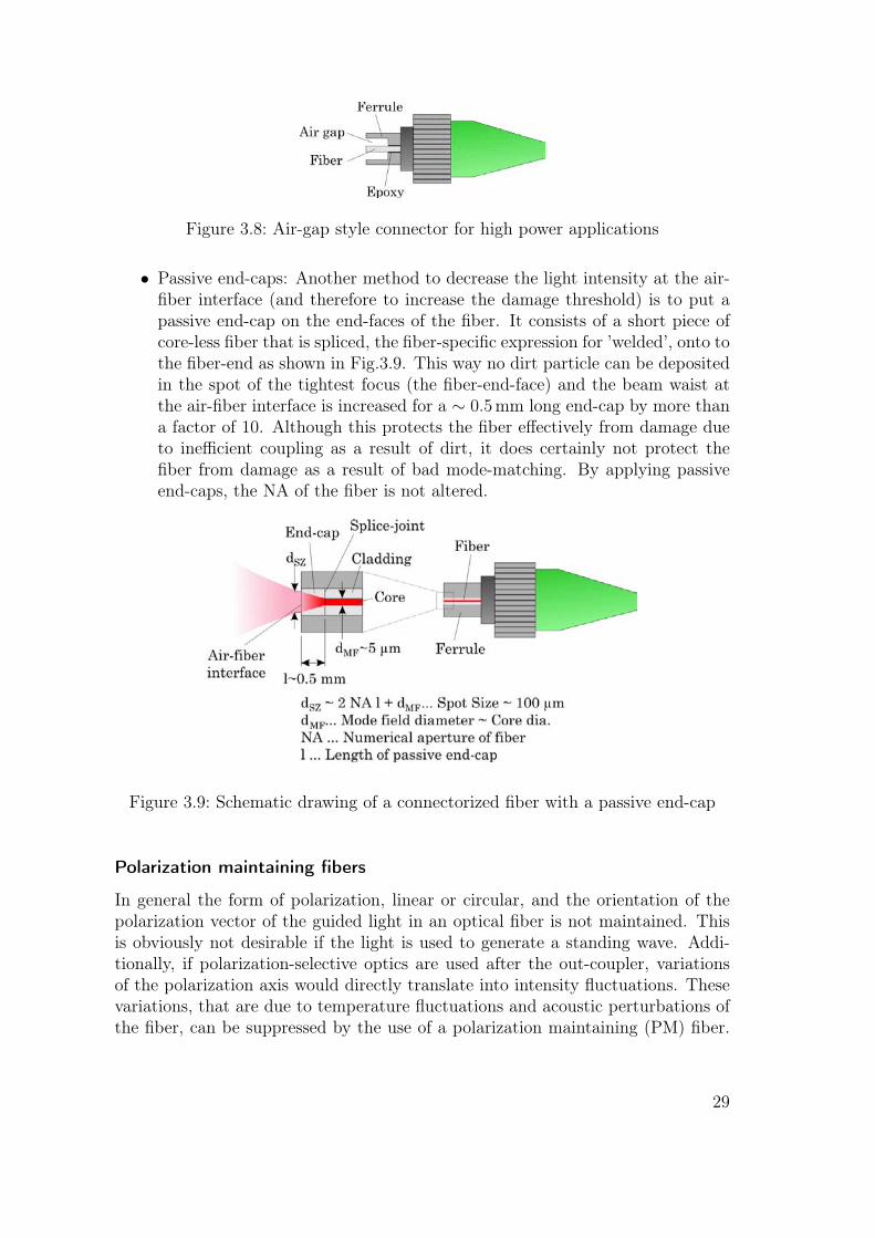
Figure 3.8: Air-gap style connector for high power applications

• Passive end-caps: Another method to decrease the light intensity at the air-fiber interface (and therefore to increase the damage threshold) is to put apassive end-cap on the end-faces of the fiber. It consists of a short piece ofcore-less fiber that is spliced, the fiber-specific expression for ’welded’, onto tothe fiber-end as shown in Fig.3.9. This way no dirt particle can be depositedin the spot of the tightest focus (the fiber-end-face) and the beam waist atthe air-fiber interface is increased for a ∼ 0.5mm long end-cap by more thana factor of 10. Although this protects the fiber effectively from damage dueto inefficient coupling as a result of dirt, it does certainly not protect thefiber from damage as a result of bad mode-matching. By applying passiveend-caps, the NA of the fiber is not altered.

Figure 3.9: Schematic drawing of a connectorized fiber with a passive end-cap

Polarization maintaining fibers

In general the form of polarization, linear or circular, and the orientation of thepolarization vector of the guided light in an optical fiber is not maintained. Thisis obviously not desirable if the light is used to generate a standing wave. Addi-tionally, if polarization-selective optics are used after the out-coupler, variationsof the polarization axis would directly translate into intensity fluctuations. Thesevariations, that are due to temperature fluctuations and acoustic perturbations ofthe fiber, can be suppressed by the use of a polarization maintaining (PM) fiber.

29

Such a fiber possesses a pair of ’stress rods’, a certain geometric variation of therefractive index in its cladding (see Fig. 3.10). These stress rods effectively createa slow and a fast axis in the fiber. If the direction of polarization of the light thatis coupled into the fiber coincides with the slow or fast axis of the PM fiber, theorientation of the polarization axis of the out-coupled light is maintained withinan angle of ±3◦ or ±5◦ respectively and the intensity fluctuations can be reducedto 3−5%. The fluctuations are usually on a minute timescale, but they can be ac-celerated (e.g. for testing) by heating the fiber, e.g. with a hair dryer. To suppressthe remaining ∼ 5% we actively stabilize the light intensity with a PI-controller.

Figure 3.10: Cross section of a polarization maintaining fiber

Coupling efficiency

Throughout this work the coupling or fiber efficiency ηcoupling simply refers to

ηcoupling =Pbefore

Pafter

,

with Pbefore and Pafter being the laser power before and after the fiber. As thedamage threshold directly depends on the coupling efficiency, some care shouldbe taken when coupling the light into the fiber. Given the numerical apertureand the core diameter of the fiber, the beam diameter and the focal length ofthe collimating lens need to be chosen accordingly. The following straightforwardrelations can be used to obtain a set of parameters [Bes99, New]:

dSZ =4λf

πdB

∼ dMF

NArays ∼dB/2

f< NAfiber

Here dSZ stands for spot size of the focused laser beam at the fiber end face, f isthe focal length of the lens used, and dB is the beam diameter at the lens. Themode field diameter dMF is a measure of the width of the guided mode and issimilar to the core diameter of the fiber. NArays is the numerical aperture of the

30

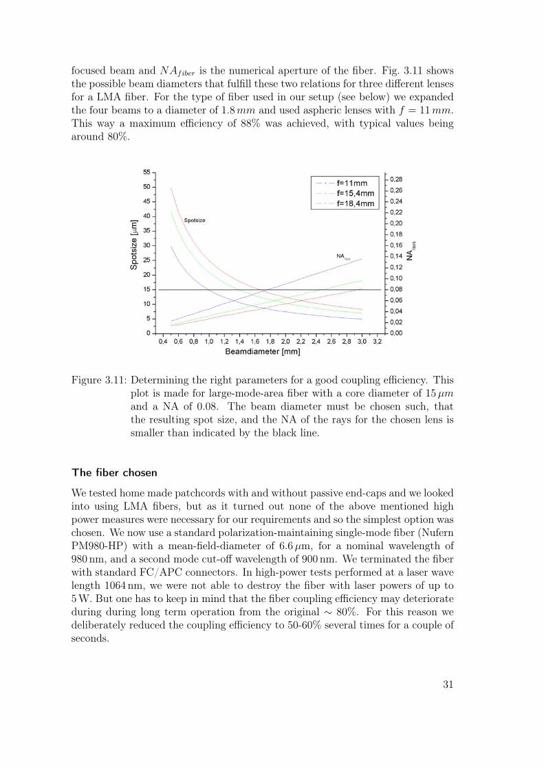
focused beam and NAfiber is the numerical aperture of the fiber. Fig. 3.11 showsthe possible beam diameters that fulfill these two relations for three different lensesfor a LMA fiber. For the type of fiber used in our setup (see below) we expandedthe four beams to a diameter of 1.8mm and used aspheric lenses with f = 11mm.This way a maximum efficiency of 88% was achieved, with typical values beingaround 80%.

Figure 3.11: Determining the right parameters for a good coupling efficiency. Thisplot is made for large-mode-area fiber with a core diameter of 15µmand a NA of 0.08. The beam diameter must be chosen such, thatthe resulting spot size, and the NA of the rays for the chosen lens issmaller than indicated by the black line.

The fiber chosen

We tested home made patchcords with and without passive end-caps and we lookedinto using LMA fibers, but as it turned out none of the above mentioned highpower measures were necessary for our requirements and so the simplest option waschosen. We now use a standard polarization-maintaining single-mode fiber (NufernPM980-HP) with a mean-field-diameter of 6.6µm, for a nominal wavelength of980 nm, and a second mode cut-off wavelength of 900 nm. We terminated the fiberwith standard FC/APC connectors. In high-power tests performed at a laser wavelength 1064 nm, we were not able to destroy the fiber with laser powers of up to5 W. But one has to keep in mind that the fiber coupling efficiency may deteriorateduring during long term operation from the original ∼ 80%. For this reason wedeliberately reduced the coupling efficiency to 50-60% several times for a couple ofseconds.

31

During operation one should always keep an eye on the evolution of the fiberefficiency. If it drops below a critical value of around 60% the transmittance oflaser powers > 1W should be avoided or at least limited to short time intervals.For this reason a whole array of photo-diodes (PD) was installed in the setup. Forevery fiber there is a PD before and after the fiber. They can be used to check thecurrent coupling efficiencies.

3.2.4 Aiming at the atomic ensemble

The preparation of a Bose-Einstein condensate with Cs atoms is in itself a majorexperimental challenge and requires a complex experimental setup [Fli06, Her05].For this purpose our setup includes 16 laser beams aiming into the experimentalchamber. Accordingly, the space around the glass cell is quite valuable, and it getssomehow challenging to find optical access to the region of interest (ROI) in theexperimental chamber. This is particularly the case for a 3D-lattice, where oneneeds optical access from both directions along three mutually orthogonal axes.But optical accessibility was one of the main requirements while planning thisthird generation Cs-BEC experiment, and therefore a glass cell was chosen (seesec. 2.3.1).

General Setup

We decided to arrange the four laser beams for the optical lattice as follows (seeFig.3.12):

• Two mutually orthogonal and retro-reflected beams oriented horizontally ata near 45◦ angle in respect to the glass cell.

• Two counter-propagating beams along the vertical direction..

Figure 3.12: Schematical drawing of the beam arrangement in respect to the ex-perimental chamber

32

The reasons for this arrangement are straightforward: The vertical beams allowfor experiments with an 1D-lattice and a variable external force (e.g. the observa-tion of Bloch-oscillations). This way we can use gravity and/or accelerate the lat-tice by slightly detuning the two counter-propagating beams. For now, the beamsdeviate about half a degree from a perfect vertical alignment, since it is blocked bythe set-up for Raman-sideband-cooling. The near 45◦-arrangement (∼ 50◦) of thevertical beams offered the simplest technical realization, and it has the advantagethat we can distinguish between the different momentum peaks in our time-of-flight(TOF) images. (The imaging axis is orthogonal to the long axis of the chamber.)

For the horizontal beams the setup is realized as shown in Fig. 3.13. This setup isinstalled at the same height as the vacuum chamber and hence some riser-platformsare required. The light is coupled out of the fiber with a waist of around 900µmand is then reduced with a pair of lenses to the desired beam-waist of 500µm atthe ROI. Two mirrors at 45◦ angle offer the necessary degrees of freedom to alignthe laser beams with the atom cloud. At the other side of the glass cell anotherpair of lenses is placed in front of the 0◦-mirror to obtain a beam-waist of 500µmfor the retro-reflected beam at the ROI. An optical isolator protects the fiber fromthe retro-reflected beam.

The setup for the vertical beams is implemented as shown in Fig. 3.14. Thebeam with the propagation direction bottom-to-top (beam Zb−t) is coupled out ofthe fiber one level below the glass cell. It passes the optical diode, three mirrors,and a pair of lenses before it is reflected upward into the ROI by a fixed 45◦-mirror.This mirror is, as it is also used for other laser beams (MOT, Raman-cooling), a 2′′

diameter broadband mirror, which only preserves polarization if the incident beamis either s- or p-polarized (see sec 3.2.2). Due to historic reasons, this 2′′ mirroris mounted such that the propagation direction of the incident beam has to beorthogonal in respect to the long axis of the experimental chamber, for the reflectedbeam to be vertical. As a consequence we were obliged to choose a polarizationaxis for the vertical lattice beams that is in ∼ 45◦ angle to the horizontal latticebeams. This current setup makes a 3D beam configuration with mutual orthogonalpolarizations, as mentioned in section 3.1.2, not possible. Since the same effect aswith orthogonal polarizations can be achieved by mutually detuning the latticeaxes, a beam configuration as shown in Fig. 3.15 was chosen. With a relativedetuning in the MHz-range, the atoms ’see’ an average potential that is basicallyidentical to one produced with mutual orthogonal polarizations (see Fig. 3.3 (b)).

The setup for the beam with the propagation direction top-to-bottom (beamZt−b) is analogous to its counter-part, except that it is arranged on the breadboardabove the glass cell (see Fig. 3.14).

The aiming process

The lattice beams in our setup have a relatively large waist of around 500µm,therefore the aiming process turns out to be quite simple.

1. Pre-alignment:

33

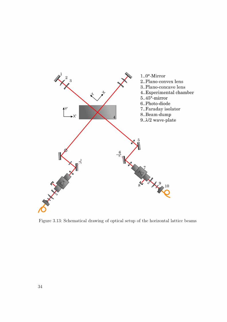
Figure 3.13: Schematical drawing of optical setup of the horizontal lattice beams

34

Figure 3.14: Schematical drawing of optical setup of the vertical lattice beams

35

Figure 3.15: Experimentally realized beam configuration including polarizationand detuning.

At first we align the beams per eye in respect to the existing -already aligned-beams (e.g. Raman-sideband-cooling). At this and the next step we doneither worry about the retro-reflected nor the counter-propagating beam byblocking the 0◦-mirror and by only using one of two Z-beams (e.g., Zt−b).

2. Alignment of incident beams:Next we aim at the atoms by using the three beams, one by one, as a simpledipole trap without forming a standing wave. We do this by producingsamples of ultracold Cs atoms with a temperature of about 1µK while shiningthe beam into the experimental chamber. By using a power of up to 2W wecan achieve a dipole potential depth of > 1µK. The effect of the beam on theatom cloud is easily seen on the absorption or even fluorescence image aftera levitated time-of-flight (TOF) of about 100 ms. As we work with relativelylarge beam waists, we were usually able to see the effect of the beam evenwith a bad pre-alignment. At this point one only needs to exactly align thecenter of the beam with the desired position. The desired position has to bepreviously marked on the absorption image. It indicates the spatial positionin two dimensions of the BEC after evaporation. For aligning the beam alongthe third dimension, we use a second camera providing fluorescence picturesof the atom cloud from a different angle. See Fig. 3.16 for typical images ofthis alignment process.

3. Alignment of the retro-reflected / counter-propagating beams:For the horizontal lattice beams we use the 0◦-mirror to couple the retro-reflected beam back into its own fiber. Even with the optical diode adjustedto maximal isolation, one can detect a very weak beam after the AOM whensufficient high powers are used (1-2W). Here, ’after the AOM’ refers to thepropagation direction of the retro-reflected beam. If the signal of this beamis maximized one can assume to have a perfect overlap of the incoming andretro-reflected beam. To find this signal one can of course deliberately de-

36

Figure 3.16: Alignment of incident beams. Two fluorescence pictures taken after alevitated TOF of 60 ms during the alignment process as described inthe text.

adjust the Faraday isolator, but one needs to keep in mind that the settings ofthe optical diode should not be changed after step 2 of this alignment-process.This is especially true for Faraday isolators with Brewster polarizators de-signed for high laser power. They introduce a substantial beam pointingerror when rotating the polarizator. The alignment is done similarly for theremaining vertical beam. So, if e.g. beam Zt−b was aligned in step 1 and 2,we now overlap beam Zb−t as good as possible with beam Zt−b, and coupleit into the fiber of beam Zt−b. The same considerations as above are valid,except that it is much easier to find the weak beam transmitted through theisolator and the second fiber, since we can now place a photo-diode directlybehind the fiber out-coupler.

37

4 BEC in an Optical LatticePotential

The first part of this chapter briefly introduces the theory describing the physicsof a BEC trapped in a 3D lattice potential. In particular the Bose-Hubbard modeldescribing the quantum phase transition from the superfluid (SF) to the Mottinsulator (MI) state is reviewed. The following section presents some of our mea-surements performed in order to test and characterize the lattice. The last sectionof this chapter reports on the observation of the SF to MI quantum phase tran-sition, as the lattice depth, i.e. the ratio between kinetic energy and interactionenergy, is varied. Additionally -and this is unprecedented- we present first indica-tions of the ability to drive the phase transition via tuning of the scattering length,i.e. as only the interaction term in the Hamiltonian is varied.

4.1 Theoretical Introduction

4.1.1 Band structure, Bloch and Wannier functions

In order to describe the effect of a periodic potential on an atom cloud, we mustfirst review the single-particle physics in such a system. As known from solidstate physics, the movement of a single particle in a periodic potential implies theemergence of a band structure.

The dynamics of a single particle in a 1D periodic potential can by described bythe Schrödinger equation

Hφ = Eφ, with H =p2

2m− V01D

cos2(kx) (4.1)

being the Hamiltonian for an atom in an 1D lattice potential, and p = −ih∇ beingthe momentum operator. According to the Bloch-Theorem (see e.g. [Kit04]), thesolutions (Bloch functions) must have the form

φnq (x) = eiqxun

q (x), (4.2)

where unq (x) are functions with the same periodicity a = λ/2 = π/k as the po-

tential. It is found that the solutions can be completely characterized by theirbehavior in the first Brillouin zone ranging from q = −hk to hk. Remember thathere k is the wavevector of the laser light field and represents the lattice constant.

39

The so-called quasimomentum q characterizes the phase difference of the particle’swavefunction between neighboring lattice sites.

Inserting this ansatz into Eq. 4.1 leads to a Schrödinger equation for unq (x):

Hqunq (x) = En

q unq (x), with Hq =

(p+ q)2

2m− V01D

cos2(kx). (4.3)

In general unq (x) are complicated functions. They can be found numerically after

expanding unq (x) and V01D

cos2(kx) as discrete Fourier sums (see Appendix B). Theeigenvectors define the Bloch functions φn

q (x). They are, as one can see in Fig. (4.2),completely delocalised over the whole lattice. The eigenvalues En

q represent theeigenenergies for the nth energy band. Figure 4.1 shows the band structure fordifferent potential depths. Depending on the lattice depth V01D

, atoms in thelowest bands (Eq

n < V01D) are in bound states of the potential, whilst the higher

bands (Eqn > V01D

) correspond to free particles. For deep lattices the potentialon each lattice site can be approximated by a harmonic potential so that thelevel spacing hωlat corresponds to the energy separation of the two lowest bandsE1

q=π/a − E0q=π/a.

The tunneling matrix element J , which describes the tunnel coupling betweenneighboring lattice sites, is directly related to the width of the lowest energy bandthrough [Jak99]

J =max(E0

q −min(E0q )

4. (4.4)

It is often convenient to express the Bloch functions in terms of Wannier func-tions [Wan37], which also form a complete set of orthogonal basis states and arewave functions that are maximally localized to individual lattice sites.1 For 1D theWannier functions are given by

wn(x− xi) =

√a

2π

∫ π/a

−π/aφn

q (x)e−iqxidq, (4.5)

where xi are the minima of the 1D lattice potential. The absolute-square of thesewave functions can be interpreted as the probability distribution of a particle inthe nth energy band that is spatially localized to the ith lattice site. The basistransformation can also be reversed to give

unq (x) =

√a

2π

∑i

wn(x− xi)e−iqxi . (4.6)

1The Wannier functions are not uniquely defined by Eq. (4.5) because each Bloch wave functionis arbitrary up to a complex phase. But for every band there exist only one Wannier functionwhich has all three of the following properties (Kohn1959):

• It is real.

• It is either symmetric or antisymmetric about either x=0 or x=a/2.

• It falls off exponentially.

Throughout rest of this work we will only refer to these Wannier functions, which are knownas maximally localised Wannier functions.

40

Figure 4.1: Band structure of an 1D optical lattice. Energy of the Bloch stateversus quasimomentum, plotted for different lattice depths. For deeplattices the lowest band becomes flat and the width of the first bandgap corresponds to the level spacing hω on each lattice site.

Figure 4.2: Probability density of the Bloch wave functions for q = 0 and q = hkin the lowest band n = 0 for different lattice depths V0. Bloch statesare completely delocalized over the whole lattice.

41

Figure 4.3: Real part of the Bloch functions in the lowest band for many differentquasimomenta q and for three different lattice depths V0. By summingthe Bloch functions of all possible q’s one obtains a localized wavefunc-tion at position xi = 0.

Figure 4.4: Probability density of a Wannier function for various lattice depths.Wannier functions constitute an orthogonal set of localized wavefunc-tions. The lattice potential is also illustrated.

42

For sufficiently deep lattices the Wannier functions for lower bound bands maybe replaced by the harmonic oscillator wave functions. The major error in thisapproximation is that the Wannier functions fall off exponentially, whereas wavefunctions of the harmonic oscillator decay more rapidly in the tails (e−x2/(2a0)2).

4.1.2 Bose-Hubbard Model

The simplest system for which one can investigate the Mott insulator phase tran-sition at zero temperature are repulsively interacting bosons with spin zero in anoptical lattice. Such a system is nicely described by the Bose-Hubbard model, anextension of the Hubbard model from solid state physics to bosonic particles. Thiswas first realized by Jaksch et al. [Jak99]. The resulting physics of the correspond-ing Hamiltonian is governed by the competition between kinetic- and interactionenergy of the strongly interacting bosons.

Bose-Hubbard Hamiltonian

The Bose-Hubbard Hamiltonian is deduced from the many body Hamiltonian de-scribing N interacting bosons confined by an external potential Vext

H =∫d3xψ†(x)

(− h2

2m∇2 + V (x)

)ψ(x) +

1

2

4πash2

m

∫d3xψ†(x)ψ†(x)ψ(x)ψ(x)

(4.7)where ψ†(x) is a boson field operator for atoms in a given internal atomic state.V (x) is the sum of the lattice potential (see Eq. 3.11) and a possible additionalexternal confinement Vext(x). Since in our setup the waists of the lattice laserbeams are much larger than the atom cloud and also much larger than the possibleexternal confinement produced by the dimple-beam, we can approximate the latticepotential (Eq. 3.11) by V (x) = V01D,x

cos2 kx+ V01D,ycos2 ky + V01D,z

cos2 kz.The second term in the Hamiltonian represents the interactions between the

atoms, with as being the s-wave scattering length and m the mass of the atom.Because we are interested in the local atom-atom interactions, it is favorable to

expand the field operator in the Wannier basis (see section 4.1.1). If one assumesthe energies involved in the system dynamics to be small compared to excitationsenergies to the second band, only Wannier functions of the lowest band have to beconsidered, so that the field operator can be written as

ψ(x) =∑

i

biw0(x− xi), (4.8)

and the Bose-Hubbard Hamiltonian reduces to

H = −J∑〈i,j〉

b†ibj +∑

i

(εi − µ)ni +1

2U∑

i

ni(ni − 1). (4.9)

Here bi and b†i denote the annihilation and creation operator for the ith lattice site,and the operator ni = b†ibi counts the number of atoms at lattice site i. The threeterms can be interpreted as follows:

43

• The first term describes the hopping (tunneling) of atoms between adjacentlattice sites, with J being the tunnel matrix element for a particle to go fromsite i to one of its nearest neighbors j. Therefore 〈i, j〉 denotes all pairs ofnearest neighbors. Delocalization of the atoms minimizes this term since (ina very simplified picture) the ground state energy of the atoms decreases asthe confinement volume increases.

• The second term accounts for the energy offset due to the external confine-ment εi =

∫d3xVext(xi)|w(x − xi))|2 ≈ Vext(xi). Please note that µ was

introduced to act as a Lagrangian multiplier when a grand canonical ensem-ble is considered. It ensures that

∑i〈ni〉 = N and represents the chemical

potential. The difference (µ − εi) can therefore be viewed as the effectivelocal chemical potential at the lattice site i.

• The repulsive interaction between particles in the same lattice site is de-scribed by the third term. Here U quantifies the cost in energy due to therepulsion of two adjacent atoms. The number of possible atom pairs in onelattice site is given by 1

2ni(ni−1). Therefore this term is reduced if the atoms

are localized to certain lattice sites.

For a given optical lattice potential the hopping matrix element J and the on-site repulsion parameter U can be evaluated numerically by calculating the bandstructure and its corresponding Wannier functions and evaluating the followingexpressions:

J = −∫d3xw(x− xi)

(− h2

2m∇2 + V (x)

)w(x− xj) (4.10)

U =4πash

2

m

∫d3x|w(x)|4. (4.11)

The dependence of J and U from the lattice depth V0 is further discussed in thenext section and can be seen in Fig. 4.8. Note that the hopping term decreasesexponentially whereas the interaction term increases slightly due to a tighter con-finement of the interacting bosons. Therefore the ratio U/J is adjusted whenvarying the lattice depth, whereas, by scanning the scattering length as the on-siteinteraction U can be tuned separately.

Solving for the ground state of Bose-Hubbard Hamiltonian in mean field theoryyields two different regimes: the superfluid phase with the number of atoms perlattice site fluctuating, and the Mott-insulator phase, where the particle numberfluctuation at each site tends to zero.

Superfluid Regime

For U/J small, i.e., for a small on-site interaction compared to energy associatedwith tunneling, the ground state is superfluid (SF). The tunneling term dominates

44

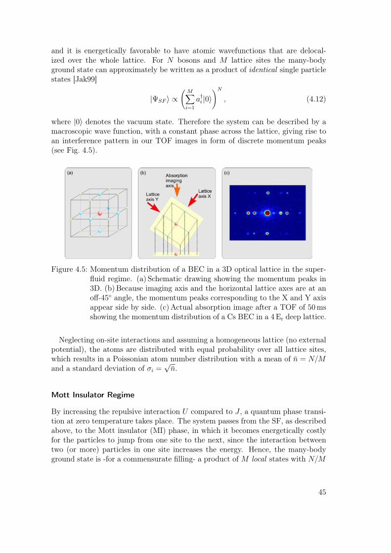
and it is energetically favorable to have atomic wavefunctions that are delocal-ized over the whole lattice. For N bosons and M lattice sites the many-bodyground state can approximately be written as a product of identical single particlestates [Jak99]

|ΨSF 〉 ∝(

M∑i=1

a†i |0〉)N

, (4.12)

where |0〉 denotes the vacuum state. Therefore the system can be described by amacroscopic wave function, with a constant phase across the lattice, giving rise toan interference pattern in our TOF images in form of discrete momentum peaks(see Fig. 4.5).

Figure 4.5: Momentum distribution of a BEC in a 3D optical lattice in the super-fluid regime. (a) Schematic drawing showing the momentum peaks in3D. (b)Because imaging axis and the horizontal lattice axes are at anoff-45◦ angle, the momentum peaks corresponding to the X and Y axisappear side by side. (c)Actual absorption image after a TOF of 50msshowing the momentum distribution of a Cs BEC in a 4 Er deep lattice.

Neglecting on-site interactions and assuming a homogeneous lattice (no externalpotential), the atoms are distributed with equal probability over all lattice sites,which results in a Poissonian atom number distribution with a mean of n = N/Mand a standard deviation of σi =

√n.

Mott Insulator Regime

By increasing the repulsive interaction U compared to J , a quantum phase transi-tion at zero temperature takes place. The system passes from the SF, as describedabove, to the Mott insulator (MI) phase, in which it becomes energetically costlyfor the particles to jump from one site to the next, since the interaction betweentwo (or more) particles in one site increases the energy. Hence, the many-bodyground state is -for a commensurate filling- a product of M local states with N/M

45

atoms per lattice site. It is approximately given by [Jak99]

|ΨMI〉 ∝M∏i=1

(a†i |0〉

)N/M, (4.13)

where N is the atom number and M the number of lattice sites. Commensuratefilling means that N/M is an integer. If the filling is not commensurate the remain-ing particles will act as a SF. Thus, a MI state in a homogeneous system is onlypossible with commensurate filling. This not necessarily true for an inhomogeneoussystem, as argued in the following section.

In the Mott insulator phase each atom is localized to a single lattice site, andthe atom number for each site is exactly determined and integer. Thus there is nocoherent matter wave function spreading across the whole lattice anymore and thephase relations between the local wave functions become arbitrary. Therefore theinterference pattern in the TOF images vanishes (see Fig 4.6).

Figure 4.6: Absorption image after a 50 ms levitated TOF showing the momentumdistribution of a BEC in a 3D optical lattice. With a lattice depth of16 Er the system is clearly in the Mott insulator regime resulting in aloss of long range phase coherence. Therefore no interference peaks arevisible.

4.1.3 Superfluid to Mott Insulator Transition

As mentioned in section 4.1.2 it is the competition between the interaction term12U∑

i ni(ni − 1) and the hopping term −J∑〈i,j〉 b†ibj in the Hamiltonian that is

responsible for the SF to MI transition. If we try to minimize the expectationvalue of the Hamiltonian 〈ψ|HBH |ψ〉 → min to obtain the most probable stateof our system |ψ〉, the interaction parameter U tends to localize the atoms tothe lattice sites, whereas the hopping parameter J tends to delocalize the atomsover the whole lattice. So, depending on the ratio U/J the system at T = 0energetically favors either the SF ground state (with atoms being delocalized overthe whole lattice) or the MI ground state (with a fixed atom number in each latticesite). The critical point (U/J)c where the system will undergo this quantum phase

46

transition is evaluated using mean field calculations [Kam93, Fis89, Ami98], andis given for a homogeneous system with one particle per site by the condition(

U

J

)c= (3 + 2

√2)z ≈ 5.8 · z, (4.14)

where z is the number of nearest neighbors lattice sites. For large occupationsn� 1 the critical value is (

U

J

)c= 4n · z, (4.15)

with n being the mean atom number per lattice site.These estimates agree well with more rigorous calculations [Els99]. The resulting

phase diagram for a two-dimensional square lattice is depicted in Fig. 4.7. It showsthe boundary between Mott insulating and superfluid phase as a function of thechemical potential µ and the hopping matrix element J , both in units of the onsiteinteraction U .

Figure 4.7: Phase diagram showing the boundary between Mott insulating (MI)and superfluid (SF) phase for a two-dimensional square lattice withz = 4 next neighbors. The figure is taken from Ref. [Els99].

At a given U/J the difference in µ between the top and bottom phase-boundarycorresponds to the energy gap ∆E in the excitation spectrum resulting froma particle-hole excitation. Therefore the tip of the lobe in the phase diagram(Fig. 4.7) corresponds to the critical transition point (U/J)c. At this point theenergy difference of particle and hole excitations (from a Mott insulator state)vanishes.

In fact, the excitation spectrum can be used to experimentally probe the onsetof the MI regime. In the SF phase the system can be excited by any arbitrarilysmall excitation, but as it enters the insulating phase, an energy gap ∆E opens upand one can only excite a particle-hole creation with perturbations corresponding

47

to ∆E = hωe, e.g., by modulating the lattice depth at a frequency fe = ∆E/h.For U � J , i.e. when deep in the MI phase, the energy gap equals the onsiteenergy U (see sec. 4.3.3).

Driving the Transition

The phase transition from the SF to the MI phase can be induced via the followingtwo experimentally accessible parameters:

• The lattice depth:A variation in the potential depth of the lattice inevitably changes the po-tential barrier height between lattice sites and therefore the correspondingtunneling/hopping rate of the atoms, but at the same time an increase ofthe lattice depth pushes the atoms closer together, which results in a higheronsite interaction energy. This energy U varies almost linearly as shownin Fig. 4.8 (a), whereas the hopping term J decreases exponentially as de-picted in Fig. 4.8 (b) as the lattice is ramped up. Therefore the ratio U/Jcan be varied over many orders of magnitude by changing the lattice depth.Figure 4.8 (c) shows U/6J plotted versus the lattice depth for different scat-tering lengths a. The expected value of ∼ 5.8 for the phase transition in athree-dimensional lattice is also shown.

• The scattering length:Because of the existence of suitable Feshbach resonances, one can control thes-wave scattering length a via the applied magnetic field strength over a widerange. A change in the scattering length directly influences the interactionproperties of the atoms, and one can therefore vary the onsite interaction en-ergy U without affecting any of the other parameters involved. Figure 4.8 (d)shows the required lattice depth as a function of the scattering length for theexpected phase transition to take place (given by U/6J ∼ 5.8).

Transition in an Inhomogeneous System

So far we have only discussed the transition in a homogeneous system as illustratedin Fig. 4.9 (a). The experimental realizations of a Mott insulator implies (so far)the use of an harmonic external potential as shown in Fig. 4.9 (b). In order todescribe the inhomogeneous situation one can use the standard approximationthat a slowly varying external potential may be accounted for by an effective localchemical potential µloc = µ − εi (see Eq. 4.9). Assuming e.g. that the chemicalpotential at the trap center µ falls into the n = 2 Mott-lobe, one obtains two Mottinsulating domains separated by a superfluid shell when moving to the boundary ofthe trap where µloc vanishes. In this manner, all the different phases that exist fora given J/U are present simultaneously. From Fig. 4.9 (c) it becomes obvious thatthe critical value of J/U depends on the distance from the trap center and that

48

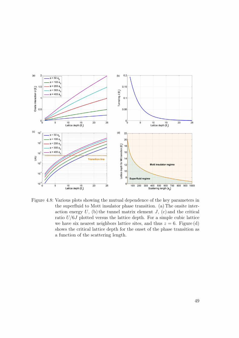
Figure 4.8: Various plots showing the mutual dependence of the key parameters inthe superfluid to Mott insulator phase transition. (a)The onsite inter-action energy U , (b) the tunnel matrix element J , (c) and the criticalratio U/6J plotted versus the lattice depth. For a simple cubic latticewe have six nearest neighbors lattice sites, and thus z = 6. Figure (d)shows the critical lattice depth for the onset of the phase transition asa function of the scattering length.

49

the transition in an inhomogeneous system is therefore continuous. Nevertheless,a rather sharp transition can be observed by ramping the lattice depth over thecritical value, because the ratio J/U depends exponentially on V0. In contrast,J/U depends only linearly on the scattering length as. Hence we expect a rathersmooth transition when raising the scattering length beyond the critical value.In any case, signatures of the SF to MI transition should become apparent fora slightly higher value U/J than predicted for the homogeneous case given inEq. 4.14. At U/J = 5.8 · z only a thin outer shell of the atomic cloud is in theMott insulating regime.

Figure 4.9: Schematic picture illlustrating a lattice with homogenous potentialdepth (a), and a system with inhomogenous potential depth (b). Eachpoint in the inhomogeneous system can approximately be viewed as ahomogeneous system with µ = µloc (c).

4.1.4 Loading of a BEC into the Lattice Potential

Adiabaticity Criteria

Most lattice experiments require the atomic ensemble to be in -or very close to-it’s many body ground state. Therefore an adiabatic transfer of the BEC into thelattice becomes substantial. If the lattice is ramped up slow enough, the wavefunction of the condensate remains in the many body ground state of the system.It is important to note the existence of two time scales of adiabaticity, i.e. one withrespect to interband transitions and the other with respect to intraband excitations.

50

• Interband: Adiabaticity with respect to the (single) particle band structure.If the lattice potential is ramped up too fast, higher energy bands can getpopulated (see sec. 4.2.2). The corresponding time scale is determined by thelevel spacing, therefore this adiabaticity criterion can be written as [Den02]

|〈n, q|∂H/∂t|0, q〉| � (Eqn − Eq

0)2/h. (4.16)

The left-hand side is always less than dV0/dt and for the case of q ∼ 0(stationary BEC) the energy difference between ground state and the firstexcitable state is at least 4Er (e.g. see band structure for V0 = 0). Thereforethe condition 4.16 (for q ∼ 0) is easily fulfilled by choosing a ramp-up speed

dV0/dt� 16E2r/h ∼ 1.3 · 105Er/s, (4.17)

meaning, that the first Er should be ramped up in a time much longer than∼ 7µs. Since the level spacing Eq

n − Eq0 increases for larger lattice depths

(V0 > 1Er), one can continuously raise the ramp-up speed and still maintainadiabaticity. See e.g. Ref. [Jul05] for the ideal ramp-up function. Note thatfor a BEC that is moving relative to the lattice potential, it becomes harderto fulfill this adiabaticity criterion, since Eq

n − Eq0 → 0 as q approaches the

Brillouin zone boundary.

• Intraband: Adiabaticity with respect to many body dynamics within thelowest Bloch band.Depending on the lattice depth and on the external confinement, the manybody ground state has a certain density profile (see below). If parameters arechanged, the atoms have to redistribute over the lattice in order to maintain aconstant chemical potential. This leads to an adiabaticity criterion with timescales that are considerably longer than discussed above. Theoretical studiesof the loading dynamics have been reported in Ref. [Skl02b, Skl02a, Ise05].An experimental study has been performed in Ref. [Ger07] in which theyfound a time scale of ∼ 100ms for adiabatically loading the BEC into thelattice. It is in accordance with the criterion |H| � ∆E2/h, where ∆E isthe energy difference between ground state and possible excitation. If wereduce the question of adiabaticity to whether the atoms can redistributethrough tunneling in order to adapt the size of the system to the instan-taneous Thomas-Fermi shape, we can take ∆E to be of the order of thehopping matrix element J . For the relevant time scales one can also assume|H| ∼ |J |, so that we obtain the following adiabaticity criterion [Ger07]:

h|J |J2

� 1. (4.18)

51

Density Re-distribution

Using the Thomas-Fermi approximation (Ekin ∼ 0) and the Gross-Pitaevskii equa-tion we obtain the usual relations for a BEC in a harmonic potential [Pit03]:

n(r) =

{ µ−V (r)g

for µ− V (r) > 0,

0 otherwise,(4.19)

µ =hω

2

(15Nas

aho

) 25

, (4.20)

n =µ

gwith g =

4πh2as

m. (4.21)

Here n(r) stands for the atom density, µ for the chemical potential, V (r) for theconfining potential, ω = 3

√ωxωyωz for the corresponding geometrically averaged

trap frequency, aho =√

hmω

the characteristic trap size, N the total atom number,as the scattering length, m the atom mass, and n the peak density at the trap centerV (r = 0) = 0. With these expressions one can calculate the density distributionn(r) = n(1− r2/R2

TF ) with the Thomas-Fermi radius RTF = 1/ω√

2µ/m (definedas the radius at which the density vanishes) for a BEC trapped in a harmonicpotential.

If we adiabatically apply a lattice potential we obviously expect these parametersto change: By increasing the lattice depth the atoms are pushed tighter together,thereby increasing the interaction energy U . In an inhomogeneous external con-finement like a harmonic trap, this increase in energy results in an broadeningof the density distribution of the atomic ensemble (see Fig. 4.10). In analogy tothe argumentation used for calculating the above expressions, we can estimate theextension and density of the atom cloud in an optical lattice as follows [Gre03]:

By applying the Thomas-Fermi approximation to the Bose-Hubbard Hamilto-nian the expectation value of the energy for a single lattice site is given by

Ei ' Vextini +U

2ni · (ni − 1). (4.22)

Therefore the chemical potential can be calculated as

µ =∂Ei

∂ni

= Vexti + Uni −U

2= const., (4.23)

where the index i refers to the position of the i-th lattice site. Note that becausethe constant term U/2 does not alter the solution, but rather complicates thealgebra, we will omit it in the subsequent calculations.

Since the extension of the cloud is much smaller than the external potential wecan approximate Vexti by a harmonic potential 1/2mω2r2, so that we can write theaverage atom number per lattice site (at lattice site i) as

ni = nl

(1− i2

i2TF

), (4.24)

52

Figure 4.10: Change in density and Thomas-Fermi radius when loading a BECinto a lattice. Because the onsite interaction augments, the chemicalpotential and therefore the extension of the cloud increases.

53

with nl = µ/U being the peak density in the lattice potential. Note that thedensity here refers to atoms per lattice site and therefore has different units thanits counterpart n, which is in atoms per volume. The spatial coordinate is nowexpressed by the lattice site i = r/(λ/2), so that iTF = RTF · (2/λ) = 1/ω

√2µ/m ·

(2/λ) fives the lattice site at which the atom number vanishes.The chemical potential µ can now be calculated by normalizing the atom number

per site ni to the total atom number N :

N =∑

i

ni '∫nid

3i =∫ iTF

0

µ

U

(1− i2

i2TF

)4πi2di. (4.25)

Since the lattice spacing is much smaller than the extension of the cloud, we canignore the discreteness of the lattice, and we obtain

µ =

(15NU(λ/2)3m3/2ω3

16√

2π

) 25

. (4.26)

Note that this result is equivalent to the one obtained above (Eq. 4.20), except thatthe interaction term is now represented through U rather than g. The factor (λ/2)3

accounts for the different units of g and U . Figure 4.11 shows the correspondingatom number per lattice site nl = µ/U at the center of the external potential asa function of the total atom number and the external trap frequency for differentonsite interactions energies U .

Figure 4.11: Plots showing the peak atom density in atoms per lattice site as afunction of the total atom number and the external trap frequency fordifferent onsite interaction energies.

54

4.2 Testing and Characterizing the Lattice

The following section reports on the experiments that were undertaken to test andcharacterize, the optical lattice.

4.2.1 Bloch Oscillations

To get a little sense of achievement after a long period of setting up and fighting theusual obstacles, we performed the simple experiment of observing Bloch oscillationsof Cs atoms in an one-dimensional optical lattice.

The early quantum theory of electrons in crystal lattices by Bloch led to thestriking prediction that a homogeneous static electric field induces an oscillatoryrather than uniform motion of the electrons [Blo29, Zen34]. These so-called Blochoscillations had been unobserved in solid state crystals for many years, because theresulting time period (∼ ps) is much larger than scattering time of the electronsby the lattice defects.

By using ultracold Cs atoms in optical lattices one can nicely make use of thefollowing advantages: the initial momentum distribution can be tailored at will, theperiodic potential can be turned on and off and is such that the resulting Blochperiod is in the millisecond range, there are no lattice defects, the decoherencecan be adjusted via the scattering length. Already in the mid 90’s Salomon etal. [BD96] reported the observation of Bloch oscillations of Cs atoms at sub-recoiltemperatures.

What are Bloch oscillations?

Bloch oscillations are a quantum effect, which arises when a particle is placed ina one-dimensional periodic potential with periodicity a under the influence of astatic force F . The dynamics are generated by the Hamiltonian

H =p2

2m+ V (x) + Fx, with V (x+ a) = V (x). (4.27)

The resulting dynamics are quite counter-intuitive in a sense that, instead of anaccelerated motion toward infinity, one observes a coherent oscillation with period

τB =h

|F |a, (4.28)

corresponding to the time required for the quasimomentum q to scan a full Brillouinzone, and with an amplitude

lB =∆

2|F |, (4.29)

where ∆ is the width of the corresponding energy band. A simplistic explanationcan be given by assuming an invariance under a translation in space by one latticeperiod and an energy shift δE = Fa, which leads to a phase shift δEt/h. At a time

55

Figure 4.12: Schematic plot showing the ramping procedure for lattice depth, lev-itation fields, and external optical potential for the observation ofBloch oscillations.

τB this phase shift will equal 2π. The available space interval for the oscillatorymotion is limited by the fact that the gained kinetic energy Fx can not be largerthan the width of the Bloch-band (see Fig. 4.1).

For a more detailed theoretical discussion of this peculiar phenomenon and itspossible applications, please refer to Ref. [TH04, Sco04, Kol04, Car05].

Experimental Observations

For this measurement we create a BEC with about 105 Cs atoms. The verticalone-dimensional optical lattice is then ramped up in 1 ms to a lattice depth of 4 Er

and all the trapping and levitation potentials are turned off (see Fig. 4.12). Atthis point the macroscopic matter wave starts evolving according to Eq. 4.27 withgravity acting as the force F = mg. After a certain lattice hold time (accelerationtime) ta the lattice is switched off and the levitation potential is turned back onfor a levitated time of flight (TOF) of 50ms. Subsequently an absorption imageis taken to reveal the resulting momentum distribution of the atom cloud. Fortechnical reasons a regular TOF of 6 ms is performed prior to taking the image.Throughout the rest of this work this short TOF will not explicitly be mentioned,it can be viewed as part of the absorption imaging process.

Fig. 4.13 shows the absorption images taken for various lattice hold times. Onecan nicely see how the momentum distribution scans the first Brillouin zone.

In the near future we certainly plan to investigate this phenomenon more thor-oughly, including the measurement of the interaction-induced decoherence of theBloch oscillations [Buc03, Wit05].

56

Figure 4.13: Bloch Oscillations: Absorption images taken after a levitated TOF of50ms revealing the momentum distribution for different lattice holdtimes.

4.2.2 Measuring the Lattice Depth

Obviously it is quite crucial to have an exact knowledge of the actual lattice depthfor any lattice experiment. Since the effective lattice depth depends on the actuallight power within the glass cell (which one can not measure directly), the actualbeam waist, and the spatial overlap of the counter-propagating laser beams, it isnecessary to verify the depth of our optical lattice potential experimentally, i.e., tohave a method for calibration.

For this purpose we use a simple procedure described in [Den02] where we quicklyturn on the lattice potential (each axis at a time) once the BEC is produced. Afterleaving the atom-cloud evolve for a certain lattice hold time th we shut off thelattice abruptly and measure the resulting momentum distribution as a functionof th.

Theoretical background

The eigenstates (Bloch states) |n, q〉 of the atom-lattice system can be expandedin a discrete plane-wave basis with momenta p = q + 2lhk and vice versa:

|n, q〉 =∞∑

l=−∞an,q(l)|φq+2lhk〉 (4.30)

|φq+2lhk〉 =∞∑

n=0

a∗n,q(l)|n, q〉 (4.31)

Figure 4.14 and 4.15 show the decompositions for q = 0 and a lattice depth of25 Er.

A BEC with a momentum spread � hk can be approximated by a plane wave|Ψ(t = 0)〉 = |φp∼0〉). When suddenly loaded into a lattice, we can re-write its

57

Figure 4.14: The lattice eigenstates can be expressed as a superposition of planewaves with fractional population |an,q(l)|2. Shown is the plane-wavedecomposition of the lattice eigenstates |n, q = 0〉 for the four lowestbands for q = 0 and a lattice depth of 25 Er.

Figure 4.15: The plane waves |φp=q+2lhk〉 can be expressed as a superposition ofBloch states |n, q〉 with fractional population |a∗n,q(l)|2. Here, the de-compositions of plane waves |φp=2lhk〉 with q = 0 for l from 0 to 3 anda lattice depth of 25 Er are shown.

58

wavefunction for convenience in the Bloch state basis |n, q〉

|Ψ(t = 0)〉 =∞∑

n=0

|n, q〉〈n, q|φp〉 =∞∑

n=0

a∗n,q(0)|n, q〉. (4.32)

The BEC wavefunction, while held in the lattice, evolves in time according to

|Ψ(t)〉 =∞∑

n=0

a∗n,q(0)e−i

En(q)h

t|n, q〉. (4.33)

After a time th we abruptly switch off the periodic potential, projecting the resultback onto the plane-wave basis, we obtain the coefficients bq(l) of each of theplane-wave components

bq(l) =∞∑

n=0

a∗n,q(0)an,q(l)e−i

En(q)h

th , (4.34)

which correspond to the populations of the discrete momentum peaks of ourTOF measurements. The resulting interferences of the differently evolving phasese−iEn/ht produce oscillations in the populations of these discrete momentum compo-nents as a function of th, e.g. for the case where only band 0 and 2 are significantlypopulated:

|bq(l)|2 ∝ 1 + cos(E2 − E0

hth). (4.35)

Band 1 and all odd bands are not populated because the symmetry of those eigen-states (antisymmetric) does not match the symmetry of the initial BEC wavefunc-tion.

Therefore the oscillation frequency f0−2 = h/(E2(q = 0)−E0(q = 0)) is a directmeasure of the energy gap between band 0 and 2, which in turn depends on thelattice depth (see section 4.1.1).

The measurement

The following procedure is performed with only a one dimensional lattice, each axisat a time. After producing a BEC with 105−2 ·105 atoms, we switch the lattice onas fast as possible. For this purpose we turn off the active intensity stabilization(PI control, see section 3.2.2). Its use would limit us to ramp-up times of around50µs. To avoid shot-to-shot fluctuations of the light intensity an initializationprocedure at the beginning of each sequence is performed. In this short procedurethe lattice and its intensity stabilization is turned on for a time > 50µs, then thedirect digital synthesis device (DDS) and thereafter the stabilization is turned off.Using this initialization procedure prior to a short unstabilized operation is almostequivalent to a stabilized operation, since the main intensity fluctuations are dueto a drift of the polarization axis (see section 3.2.3), which are on the order of 30 swhereas the time between initialization and actual use of the lattice is on the orderof 5 s (the time it takes to produce a BEC).

59

Without active stabilization the ramp-up time is only restricted by the DDS(bus-tact frequency) and therefore the ramp-up time should be of the order of5µs (a measurement of the actual ramp-up time is currently limited by the muchslower photo-diodes). The After a lattice hold time th the potential is turned off byswitching off the DDS. To reveal the momentum distribution, an absorption imageis taken after a levitated TOF of 50ms. During the entire sequence the atoms arelevitated using the appropriate magnetic fields.

Fig. 4.16 and Fig. 4.17 show the time evolution of a cesium BEC in a 1D latticepotential for the X-axis and Z-axis respectively. Because of the moderate latticedepth only band 0 and 2 are significantly populated, which results in a sinusoidalvariation with frequency f0−2 of the population of the momentum components0,±2 hk. See Fig. 4.18 for the relation between frequency f0−2 and lattice depthV01D

.

Figure 4.16: Time evolution of a BEC in an abruptly ramped 1D lattice (X-axis)with a laser power of 440mW (measured before the glass cell). Thefigure on the left shows a sequence of absorption images. The ploton the right shows the populations of the momentum components(0hk,±2hk) taken for different lattice hold times th. Damped sinu-soidal functions are fitted on the data points (solid lines) and theresulting average oscillation frequency is given in the plot.

Table 4.1 shows the results of our calibration measurements for all three latticeaxes. Note that this calibration has to be redone once in a while but especiallyafter any re-alignment of the lattice beams.

Note that the high reflection loss of the lattice beam in X-direction is due to theunfavorable orientation of the polarization with respect to the glass cell. Given the

60

Figure 4.17: Time evolution of a BEC in an abruptly ramped 1D lattice (Z-axis)with a laser power of 250mW per beam. The figure at the bottomshows a sequence of absorption images. The plot at the top showsthe populations of the momentum components (0hk,±2hk) taken fordifferent lattice hold times th. Damped sine-functions are fitted on thedata points between 0.2ms and 0.4ms (solid lines). To test the fit andthe coherence of the oscillations some points were taken with higherlattice hold times. The resulting oscillation frequency favg

0−2 (averagedover the three fit-results) is also given in the plot.

61

Figure 4.18: Two plots at different scales showing the energy gap between Blochband 0 and 2 and the corresponding frequency f0−2 as a function ofthe lattice depth V01D

. Both plots are calculated numerically with theHamiltonian truncated for |l|>5 (see Appendix B).

abundant laser power, it was chosen this way to ensure that it does not interferewith the lattice beam in Y-direction. Since the X- and the Y-beam are mutuallydetuned to each other by 5 MHz, one could reduce the losses of the beam in X-direction by rotating its polarization by 90◦ without affecting the form or stabilityof the lattice potential.

4.2.3 Lattice-induced Heating

When working with a Bose-Einstein condensate, it is obviously very importantto avoid heating of the atomic ensemble. Heating can be caused by technicallimitations of the experimental setup e.g., intensity or spatial fluctuations of thelaser beam used to trap the atoms. For conventional optical dipole traps [Geh98]it is fairly easy to keep these fluctuations below the critical limit. But for opticallattice potential the technical stability requirements are more stringent, since phasefluctuations of the light field can also cause heating as illustrated in Fig. 4.19. Thesephase fluctuations can be caused by the laser source, the rf-driver of the AOM,or even by mechanical vibrations of the opto-mechanical components, i.e. mirrormounts, etc.

Therefore it is necessary to test the effect of the optical lattice on the BEC interms of heating. Such a test is in principle straightforward and can be performedin many different ways. Here we measure the remaining BEC fraction after thelattice is switched on for a certain amount of time. Obviously one should take careto meet the adiabaticity criteria for ramping the lattice up and down.

62

Axis P(1)beam Reflections Expected V01D

Measured V01DPbeam/Er

X 440mW 38%(2) 11.2Er 9.37± 0.17Er 47.0mW/Er

Y 360mW 3%(3) 14.4Er 8.67± 0.31Er 41.5mW/Er

Z 250mW (5) 8%(4) 9.5Er 7.8± 0.2Er 32.1mW/Er(1) Laser beam power measured before glass cell, (2) calc. for s-polarized @ 40◦(3) calc. for p-polarized @ 50◦, (4) calc. for 0◦ incident beam angle, (5) per beam

Table 4.1: Summary of the lattice depth measurements. For comparison theexpected lattice depth, including the loss due to reflections on theglass cell, is also given. Any discrepancy between expected and mea-sured values are most likely due to misalignment of the incoming andreflected/counter-propagating laser beams and/or the actual beam waistdiffering from the supposed 500µm.

Figure 4.19: Phase fluctuations in the laser light field can cause heating of theatoms trapped in the standing wave. Phase fluctuations can originatefrom the laser source, the rf-driver of the AOM, or from mechanicalinstabilities of the opto-mechanical setup. Phase fluctuations translateinto a spatial movement of the lattice wells. If this movement has aperiodicity of the trap frequency of the lattice well, it will contributeto the heating of the atomic ensemble.

Experimental Sequence

The starting point is a BEC with about 1.5 · 105 atoms. The lattice is rampedup exponentially at a constant rate, according to V0(t) = 10Er · et/100 ms. Thisway, the first part of the ramp is the same for different final lattice depths, andthe different measurements can be compared even if adiabaticity is not completelyfulfilled. Then the lattice is held a certain depth V0 for a variable time th, before itis linearly ramped down to zero in 120ms. See Fig. 4.20. Now, a TOF absorptionimage with an expansion time of 50ms is taken. The BEC fraction of the atomcloud is extracted from the image by applying a bimodal fit [Sel04] as shown inFig. 4.21. The bimodal fit accounts for the fact that the BEC is at the center of thecloud, and that its density distribution is given by the Thomas-Fermi parabola.The atoms that are not in the absolute ground state surround the BEC. Thisthermal fraction is fitted by a Gaussian distribution.

63

Figure 4.20: Ramping of the lattice depth for the measurement of lattice-inducedheating. The ramp up is performed exponentially with a constantrate to ensure the same adiabaticity condition for different final latticedepths during the critical first part of the ramp.

Figure 4.21: Determining the BEC fraction: (a) Absorption image taken after aTOF of 50 ms. (b) Bimodal fit: The BEC fraction is determined bythe area under the TF-parabola divided by the area of the total fit.

64

Observations - 3D Lattice

Figure 4.22 shows the BEC fraction plotted versus the lattice hold time th fordifferent lattice depths V0. For comparison one measurement was made with zerolattice depth. The BEC fraction grows in the first 2 s by almost 20%, indicating anincomplete evaporation during the BEC production sequence. For a shallow lattice(4Er) some heating effect can already be observed. For a lattice depth of 13Er theBEC fraction is substantially reduced on the timescale of 500 ms, a timescale thatis about an order of magnitude larger than the longest lattice hold time performedin any of the experiments presented within this work. Nevertheless, for futureexperiments longer lattice hold times may be required. Therefore the exact causesof the heating and possible improvements have to be investigated.

Figure 4.22: Plot showing the remaining BEC fraction after holding the atoms inthe 3D lattice for a time th for various lattice depths.

In summary we conclude that the lattice-induced heating of the 3D lattice is atthe order of 0.5%

100ms 1Erfor now.

Observations - 1D Lattice

As a second step, the heating caused by each individual lattice axis was examined.In Figure 4.24 (a) the remaining BEC fraction is plotted against the lattice holdtime for a depth of 8Er. At first sight it seems as only the lattice along the X-axis is responsible for the heating observed in the 3D lattice, as the BEC fractionremains more or less constant for the Y, and Z-axis. But, by also plotting theremaining total atom number versus the lattice hold time, see Fig. 4.24 (b), one canobserve a stronger atom loss while holding the atoms in the Z-axis. At this point

65

we attribute this behavior to the following circumstances: The external confiningpotential, generated by the two dimple beams, allows for continuous evaporationonly along one direction (see Fig. 4.23), the X-axis. So, if a given lattice beam doesdisturb the atomic ensemble in its ground state, it will either cause a reductionof the BEC fraction or a reduction of the total atom number, depending on itsrelative orientation to the dimple potential. The 1D lattice in X-direction inhibitsthe continuous evaporation along its direction, resulting in the reduction of theBEC fraction. On the other hand the 1D lattice generated by the beams alongthe Z-axis does not inhibit the continuous evaporation, because the atoms withsufficient energy to overcome the dimple potential, can escape along the X-axis.Hence, the BEC fraction remains almost constant, while the total atom numbercontinuously decreases. When loading the BEC into the 1D lattice along the Y-axis, we observe neither a decrease in the BEC fraction nor to a substantial loss inatom numbers.

At this point we do not fully understand as to why the 1D lattices along the Y-axis hardly influences the BEC, whereas the beams along the other two directionsdo have an observable effect on the atomic ensemble.

Figure 4.23: Schematic plot showing the shape of the external potential created bythe two dimple beams.

66

Figure 4.24: Effects of each individual 1D lattice on the atomic ensemble. The BECfraction (a) and the total atom number (b) after holding the atoms ina 1D lattices is plotted as a function of the lattice hole time for eachindividual lattice direction. For comparison the effect of the 3D latticeis also shown. The measurement was performed with a lattice depthof 8Er.

67

4.3 Experimental Observations of the MottInsulator Transition

4.3.1 Driving the Transition via the Lattice Depth

Experimental Sequence

The experiments are performed with a condensate of about 1.5 · 105 Cs atoms inthe (F = 3,mF = 3) state. After evaporation process is completed (see sec. 2.3.2),the atoms are trapped by the two crossed dimple beams , where one has a waistof ∼ 40µm with a power of 1.5 mW and the other has a waist of ∼ 250µm with apower of 1000 mW. They generate an approximate harmonic trap with the followingtrap frequencies: νx = 20 Hz, νy = 18 Hz, and νz = 27 Hz. During evaporation andthroughout the rest of this experimental sequence, the gravitational potential iscompensated by an appropriate magnetic field gradient.

After the condensate has been prepared, the 3D lattice potential, as describedin sec. 3.2, is superimposed. The lattice depth is exponentially ramped up in60 ms to V0,max = 16Er. At this depth and with a scattering length of 210 a0

the peak atom number per lattice site (corresponding to the SF phase) nl = µ/Ucalculates to approximately 1.3 (see sec. 4.1.4. We therefore expect the trap centerto be in the n = 2 Mott-lobe. The atoms are held for a time th = 10 ms before thelattice is linearly ramped down again. Figure 4.25 (a) illustrates the ramping of thelattice depth. As the depth is ramped up, parts of the atom cloud (inhomogeneoussystem) will undergo a transition from the superfluid to the Mott insulator state.In this state, the tunneling of the atoms is greatly suppressed, and the long rangecoherence of the condensate is lost. If the lattice is ramped below the transitionpoint again, the system restores the phase coherence.

Long Range Phase Coherence

The long range phase coherence of the condensate in the optical lattice can bedirectly tested by observing the multiple matter wave interference pattern. Itis formed after ballistic expansion when all trapping potentials are switched offabruptly. The levitation is kept on, to keep the cloud from falling out of thecamera’s viewing range. After an expansion time of 35ms an absorption imagesis taken. If the condensate is superfluid, the resulting TOF image shows thecharacteristic momentum peaks at ±2hk. If the system is the Mott insulatorregime, the interference peaks in the TOF image vanish [Zwe03, Gre02a].

Observations

To observe the phase transition from the superfluid to the Mott insulator state, wetake levitated TOF-images at various stages of the sequence. TOF-images in theramp-up phase are taken with a sequence as shown in Fig. 4.26 (a). For imagesduring the ramp-down phase a ramping sequence as illustrated in Fig. 4.26 (b) is

68

Figure

4.25:Superfluidto

Mott

insulatortransition:

(a)Schematicaldraw

ingofthe

ramping

procedureofthe

latticedepth.

(b),(c),

and(d)T

OF-im

agestaken

atdifferent

stagesof

thesequence

forvarious

scatteringlengths.

Narrow

interferencepeaksshow

thelong

rangephase

coherenceand

thereforethe

superfluidityofthe

condensate,whereas

theabsence

ofinterferencem

axima

indicatesthe

transitionto

theM

ottinsulator

phase.

69

used. Figure 4.25 (c) shows a series of TOF-images taken with a scattering lengthof 210 a0. For a lattice depth up to about 8Er nearly perfect phase coherencecan be observed, characterized by narrow interference maxima. As the latticepotential is raised, the higher order interference maxima initially increase, becauseof a tighter localization of the atomic wave functions at a single lattice site. Ata potential depth of 12Er the interference peaks have not further increased instrength. Instead, an incoherent background shows up and gains more and morestrength as the lattice depth is raised higher. At a depth of 16Er the higher ordermomentum peaks have basically vanished, indicating the full loss of long rangephase coherence. Figure 4.25 (d) shows a similar series of TOF-images taken witha scattering length of 400 a0. Due to the higher onsite interactions, the phasetransition already takes place at a lower lattice depth. In the sequence with thescattering length set to 100 a0, shown in Figure 4.25(b), long range phase is stillpresent even for 16Er, indicating that the system is not deep in the Mott insulatorregime.

Figure 4.26: Ramping procedure for the lattice depth. (a) For a TOF image takenin the ramp-up phase. (b) For a TOF image taken in the ramp-downphase.

Comparison with the expected transition point

The exact determination of the transition point for an inhomogeneous system isa non-trivial issue [Zwe03, Kas02]. As already discussed in sec. 4.1.3, we expectany signature related to a superfluid to Mott insulator transition to appear forU/6J ∼ 5.8. Figure 4.27 shows the values of the lattice depth and scattering lengthof this measurement in the phase diagram. For the measurements with 210 a0 and400 a0, corresponding to Fig. 4.25 (c) and (d), 16Er were clearly sufficient to enterthe Mott insulater regime. This is in good agreement with the total disappearanceof the interference peaks in the TOF-images. According to this diagram, eventhe measurement performed with 100 a0 should have, at least partially, enteredthe Mott insulating phase. As we are not capable to spatially resolve the differentphases within the atomic cloud, the question remains to whether or to what extendthe system has performed the phase transition.

70

Figure 4.27: Relevant parameters for the SF to MI transition corresponding to theTOF-images shown in Fig. 4.25. The transition line in this plot is fora homogeneous system with n = 1, i.e. U/6J = 5.8, therefore onlyindicating the onset of the continuous phase transition.

4.3.2 Driving the Transition via the Scattering Length

Experimental Sequence

The starting point for this experiment is the same as described in the previoussection: A condensate of about 1.5 · 105 Cs atoms which is optically trapped bythe two dimple beams.

With the scattering length set to 170 a0, the lattice potential is adiabaticallyramped up to 9Er in 200 ms. At this point the ratio U/J and therefore thesystem is deep in the superfluid regime. In contrast to all previous experimentalrealizations of a Mott insulator, we now intend to drive the phase transition byvarying only the interaction term U via the scattering length as. In our setup, as

can be directly changed via Feshbach tuning as described in sec. 2.2.2. Thereforethe current in the magnetic coils is raised from 8.2 A to 10.5A. This correspondsto ramping the scattering length from 170 a0 to 420 a0. At this stage the systemshould be in the Mott insulator regime, resulting in a loss of the long range phasecoherence. It can be restored by ramping down the scattering length again. Themomentum distribution is imaged via a levitated TOF sequence with an expansiontime of 40 ms and a scattering length of 30 a0. Setting the scattering length to lowvalues during the expansion yields more pronounced interference maximas. Theramping procedures are illustrated in Fig 4.28.

71

Figure 4.28: Ramping procedure for lattice depth and scattering length for drivingthe system from the superfluid to the Mott insulator regime and backvia the scattering length.

Observations

Figure 4.29 shows TOF images at various stages of this sequence. At a scatteringlength of 190 a0 excellent phase coherence can be observed, as even the next higherorder interference peaks are visible. As the scattering length is increased, thestrength of the momentum peaks decreases and the incoherent background gainsconsiderably in strength and size. The increase in interaction strength makes a de-localization of the atoms over several lattice sites energetically unfavorable. There-fore the long range phase coherence and its related interference pattern disappears.At a scattering length of 420 a0 the momentum peaks have almost completely van-ished and the TOF image is dominated by a diffuse momentum distribution. Atthis point the ratio U/6J is approximately 6. To drive the system deeper intothe Mott insulator regime a higher scattering length would be required. Due totechnical reasons, this was yet not possible without decoherence effects, but itsrealization is currently worked on.

Comparison with the expected transition point/Required improvements

Figure 4.30 visualizes the parameters corresponding to the TOF-images in Fig. 4.29 (b)within the phase diagram. With a scattering length of 420 a0 and a lattice depthof 9Er we barely crossed the transition line. Thus it is even more surprising thata clear decrease in long range phase coherence is already present. As mentionedin sec. 4.1.3, one expects only a thin shell of the atomic cloud to have entered theMott insulating regime.

72

Figure

4.29:Superfluidto

Mott

insulatortransition

fora

tuningof

theinteraction:

(a)Schematicaldraw

ingof

theram

pingprocedure

ofthelattice

depthand

scatteringlength.

(b)TO

Fim

agestaken

atdifferent

stagesofthe

sequence.N

arrowinterference

peaksshow

thelong

rangephase

coherenceand

thereforethe

superfluidityofthe

condensate.T

hevanishing

oftheinterference

maxim

aindicates

theonset

oftheM

ottinsulator

regime.

73

Figure 4.30: Relevant parameters for the SI to MI transition corresponding to theTOF-images shown in Fig. 4.29. The transition line in this plot is fora homogeneous system with n = 1, i.e. U/6J = 5.8, therefore onlyindicating the onset of the continuous phase transition.

4.3.3 Probing the Excitation Spectrum

The existence of the Mott insulator phase can also be nicely demonstrated byprobing the excitation spectrum. In the Mott insulating regime the atoms arelocalized to a single lattice site. When deep in the MI regime, i.e. U � J , smallexcitations of the system can only be achieved with energies in multiples of U .It corresponds to the energy cost due to onsite interaction if an atom hops to anneighboring lattice site (see Fig. 4.31). Therefore one expects to see an enhancedheating of the atomic ensemble only for excitations that correspond to multiplesof the onsite interaction U .

Experimental Sequence

To probe the excitation spectrum we load the BEC into the lattice potential. Thenthe potential depth V0 is sinusoidally modulated by 20% with a frequency fmod fora duration of 50 ms (see Fig. 4.32). This can be easily accomplished by modulatingthe laser intensity of one of the lattice beams via its AOM. For this we vary theamplitude of the appropiate rf-generators (DDS) sinusoidally. After the excitationthe lattice is ramped down, and the momentum distribtuion of the cloud is imagedwith the usual levitated TOF procedure. We characterize the heating of the atomsby the spatial extension of the cloud after an expansion time of 50 ms at a scatteringlength of 30 a0. This way the change in kinectic energy due to the excitation isbetter measurable.

74

Figure 4.31: Various excitation possibilities and their corresponding change inonsite-interaction energy.

Figure 4.32: Ramping and modulation procedure of the lattice depth. To obtainthe excitation spectrum, the width of the cloud was measured as afunction of the modulation frequency.

75

Observations

Figure 4.33 (a) shows the excitation spectrum for a lattice depth of 5Er. Atthis depth the system is still superfluid and therefore no resonance peaks arepresent. For the spectrum shown in Fig. 4.33 (b) the lattice was ramped up to13Er. Here the system is in the Mott insulator regime, and one can clearly rec-ognize two resonance peaks, one at 1060Hz and one at 2100 Hz, corresponding toU = hfmod = 0.80Er and 2U = 1.58Er. The resulting value for U agrees well withthe theoretically expected value as plotted in Fig. 4.35. For this measurement thescattering length as is set to 300 a0. Additionally a series of measurements withdifferent values is performed. The scattering length is adjusted to the desired valuetoward the end of the evaporation process, and is left constant during the wholeramping sequence of the lattice. For the levitated TOF expansion it is always setto 30 a0.

Figure 4.33: Excitation spectra while in the superfluid phase (a), and while in theMott insulator phase (b). In (a) no resonance peaks are visible, whilein (b) two peaks corresponding to 1U and 2U are present. Bothspectra are taken with the a scattering length of 300 a0.

Figure 4.34 shows the excitation spectra for various other scattering lengths.The position of the resonance peaks is obtained by fitting a double Gaussian tothe data points. The extracted values for U are plotted versus the scattering lengthin Fig. 4.35. The plot exhibits the expected linear dependence from Eq. 4.11, butit also seems to indicate that the calibration of the lattice depth was a bit offfor this measurement. A new lattice depth calibration measurement, as described

76

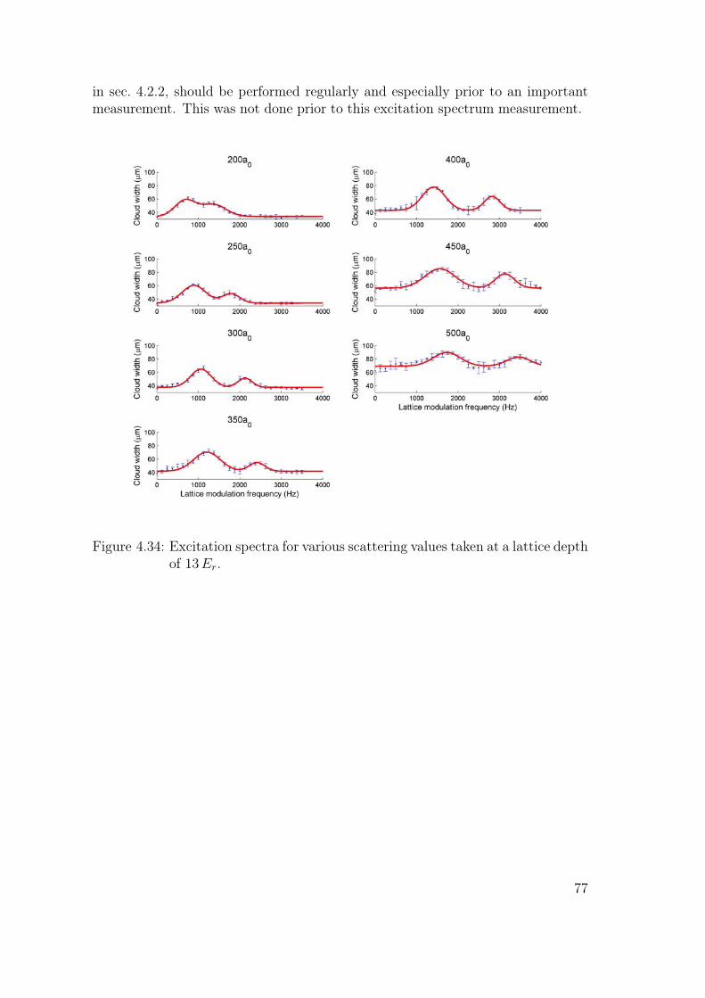
in sec. 4.2.2, should be performed regularly and especially prior to an importantmeasurement. This was not done prior to this excitation spectrum measurement.

Figure 4.34: Excitation spectra for various scattering values taken at a lattice depthof 13Er.

77

Figure 4.35: Measured onsite interaction energy U obtained from the spectra shownin Fig. 4.34 versus the scattering length. The calculated dependencefor 12Er and 13Er is also shown.

78

5 Summary and Outlook

This diploma thesis describes the work on the experimental implementation ofa three dimensional optical lattice and the realization of the superfluid to Mottinsulator transition. The light provided by a fiber-amplified narrow band laser(1064 nm) is split into four beams. The light intensity of each beam can be con-trolled via an AOM that is driven by an amplified direct digital synthesis device(DDS). This way the light intensity and therefore the lattice depth of each latticeaxis can be addressed individually with a time resolution of 5µm. To cancel anyintensity fluctuations, the intensities are stabilized using PI-control devices. Thelaser light of the four beams is guided to the experimental chamber using foursingle mode polarization maintaining fibers each with a length of 3 to 6 meters.The optical fibers are terminated in-house with FC/APC connectors. At the glasscell the four beams are arranged to create a simple cubic lattice at the center ofthe atom trap. Two beams are retro-reflected to generate two mutual orthogonalstanding waves (horizontal). The standing wave along the third lattice axis (ver-tical) is created by two counter-propagating beams. This way the lattice can beaccelerated along the vertical direction. To avoid interference effects caused bymutual orthogonal beams, the laser light along the three lattice axes is mutuallydetuned in the MHz-regime. Therefore we obtain three mutual orthogonal 1Dlattice potentials that can be used independently to create a 1D, a 2D, or a 3Dlattice. The vertical 1D lattice is tested in a first measurement by the observationof Bloch oscillations.

The waist of the lattice beams (500µm) are chosen to be relatively large com-pared to the BEC diameter (≤ 40µm), generating a relatively homogeneous latticepotential for the atoms (if no external potential is turned on). For our setup, alaser power (after the optical fiber) of about 40 mW/Er per beam is required. Weemploy the method presented in [Den02] for the a calibration of the lattice depth.Currently a maximal lattice depth of 25− 30 Er can be achieved. On a long timescale (weeks) the maximal lattice depth is currently limited by some sort of a ther-mal lensing effect. As the other main characterization measurement the heating ofthe BEC in the lattice is determined. The decrease of the BEC fraction while heldin 3D lattice is determined to be approximately 0.5%

100ms 1Er.

In preliminary measurements we are able to drive the superfluid to Mott insu-lator quantum phase transition by ramping the lattice depth as done in [Gre02a].The vanishing of the characteristic momentum peaks, attributed to the loss oflong range phase coherence, can be observed as the lattice depth is ramped up.The interference pattern can be restored by ramping the lattice depth below thetransition point. Additionally -and this is absolutely new- we present promising

79

indications that we are able to drive the SF to MI transition by tuning the scat-tering length, i.e. the interaction energy. In yet another experiment we probe theexcitation spectrum of the system in the MI regime as a function of the scatteringlength.

In summary we have implemented a 3D lattice that fulfills the proposed re-quirements and, as shown in this work, is ready to be used for novel experimentsinvolving a tunable BEC in a lattice potential. For a solid interpretation of ef-fects observed on a long time scale, a thorough characterization of the lattice-potential’s imperfections which are possibly caused by technical limitations is nec-essary. Among other, the mechanical stability of the optical setup is currentlyinvestigated. Also the parameters for ramping the lattice depth are examined inmore detail, as the intraband adiabaticity criterion might be more stringent thanpreviously assumed, especially for 1D lattices [McK06].

For the immediate future various opportunities for experiments involving a tun-able Cs BEC in an optical lattice exist. They include:

• Measurement and characterization of interaction-induced dephasing of Blochoscillations in a 1D lattice potential [Buc03]. Condensed Cs atoms allow anarrow momentum spread in combination with minimal dephasing by switch-ing the interaction strength to zero. In fact, residual dephasing could be usedas a measure to determine the strength of weak interactions. This would beparticularly important in view of an atom interferometer relying on near-zerointeraction strength.

• To drive the SF to MI transition deep into the MI regime and back withtunable interactions. An improved version of the measurement described insec. 4.3.2.

• Controlled production of molecules in the ground state of the lattice poten-tial. The MI state allows to prepare the amazing condition where preciselytwo atoms are located in each lattice site. This makes an controlled asso-ciation of dimer molecules possible, as recently demonstrated for the caseof Rb atoms on a narrow Feshbach resonance near 1000 G [Tha06]. For Csatoms with sufficiently broad Feshbach resonances at low magnetic fields,further control is within reach because it will be possible to tune onto theresonances in contrast to mere sweeps, for example near the 48 G resonance.Also, the rich molecular structure can be exploited for realization of molecularinterferometers [Mar07] in the presence of the lattice and for the controlledinvestigation of molecular Feshbach resonances [Chi05].

The intermediate and long term goals involving the optical lattice include:

• Measurement of collisional properties for two atoms at a time. In view ofthe importance of Cs atoms for atomic clocks and for fundamental reasonsthe collisional properties for Cs atoms in states other than the hyperfinequantum state F = 3, mF = 3 can be mapped out. For this, one would

80

prepare the ideal situation of precisely two ground state atoms per latticesite. Radio-frequency pulses and appropriately chosen magnetic fields canthen transfer (coherently) the full population into any desired hyperfine state,in particular into the clock state F = 3, mF = 0, allowing a measurementof the so-called clock shifts [Leo01] in the regime of ultralow temperatures.Such state-transfer techniques could be used to test the feasibility of BECin other hyperfine states of the Cs atom, and for the search of new Feshbachresonances.

• Measurement of collisional properties for three atoms at a time. In light ofthe recent evidence for Efimov quantum states [Kra06], it should be possibleto investigate the formation and stability of Efimov trimers in the presenceof a lattice [Sto05]. Interferometric techniques might even give informationon the three-body collisional phase. A full observation of Efimov’s scenariomight be possible near broad s-wave Feshbach resonances at 550 G and 800 G.

Another exciting line of research will be the realization of atom interferometersfor the precision measurement of fundamental constants, e.g. the fine structureconstant α [Gup02]. Atom interferometers rely on the matter wave diffraction ofatoms from a grating in the form of one-dimensional standing laser waves, andthey are thus in a natural connection with the matter waves in optical latticesas outlined above. A prime advantage of Cs is again the possibility to tune theinteraction strength by tuning the scattering length as, in this case to minimizethe mean-field interaction of the condensate.

81

82

Appendix A

83

84

Appendix B

Calculating the Bloch and Wannier functions

In sec. 4.1.1 we obtained the following Schrödinger equation for unq (x) by inserting

the Bloch ansatz into the time independent Schrödinger equation:

Hqunq (x) = En

q unq (x), with Hq =

(p+ q)2

2m− V01D

cos2(kx). (5.1)

This appendix points out how this equation was numerically solved using MAT-LAB, to obtain some of the plots that are shown within this work.

Since the potential V and the functions unq (x) are periodic with the same peri-

odicity, they both can be written as discrete Fourier sums:

− V01Dcos2(kx) cos2(kx) = −V01D

(e2ikx + e−2ikx + 2

)(5.2)

unq (x) =

∑l

cn,ql el2ikx (5.3)

Inserting 5.2 and 5.3 into 5.1 yields

1

2m

∑l

(2lhk + q)2cn,ql el2ikx −

∑l

V01D

4cl−1l

n,qel2ikx −∑

l

V01D

4cn,ql+1e

l2ikx −

−∑

l

V01D

2cn,ql el2ikx =

∑l

Enq c

n,ql el2ikx. (5.4)

Because all el2ikx are mutual orthogonal functions, we obtain l equations that mustbe fulfilled independently. They can be written in matrix form as follows

. . . ...· · · A−1 + C B 0

B A0 + C B0 B A+1 + C · · ·

... . . .

...cn,q−1

cn,q0

cn,q+1...

=

...cn,q−1

cn,q0

cn,q+1...

Enq , (5.5)

where Al = (2lhk+q)2

2m, B =

−V01D

4, and C =

−V01D

2, or Al = (2l + q)2, B =

−V01D

4Er,

and C =−V01D

2Erif we want the energies to be in units of recoil energies Er and the

quasimomentum in units of hk.Hence, the eigenvalues En

q of this matrix represent the eigenenergies in the nth

energy band. The corresponding eigenvector cn,q defines the appropriate Blochwave function through 5.3 and 4.2. This eigenwert problem can simply be calcu-lated if the matrix is truncated for large positive and negative l, e.g. a restrictionto −5 ≤ l ≤ 5 is a good choice if only the lowest energy bands are to be considered.Note that the term C creates only an energy offset and can therefore be chosen

85

arbitrarily or omitted. The sign of term B is also irrelevant for the dynamics ina homogeneous lattice, since writing V with sin2 instead of cos2, would yield theopposite sign for B.

The following is a MATLAB code that plots the energy band structure, the Blochfunction of the lowest energyband for different values of q, the absolute square of theBloch and Wannier functions of the lowest energy band for various lattice depths.It also plots the tunneling matrix element J and the onsite interaction energy Uas a function of the lattice depth V0. Further, the plane wave decomposition of theBloch function with q = 0 for the lowest four bands is plotted.

clear%***************Variablendekleration*********************************hbar=1.0545726*10^-34;m=133*1.6605402*10^-27;a0=5.2917725*10^-11;as=200*a0;lambda=1064*10^-9;k=2*pi/lambda;Er=hbar^2*k^2/2/m;%indizes von V0_vec, von denen Blochbänder,V0_plot=[1 6 16]; %-funktionen, und Wannierfkten geplottet werden sollenV0_max=25; %lattice depthV0_unt=V0_max; % unterteilungen von V0 (rechnet also für jedes Er aus)V0_vec=linspace(0,V0_max,V0_unt+1);

l_tot=5; %größe vom hamilton operatorl_vec=linspace(-l_tot,l_tot,2*l_tot+1);

xi_range=2; %xi=x/a von e.g. -3 bis +3 gitterplätzenxi_unt=100; %unterteilungenxi_vec=linspace(-xi_range,xi_range,xi_unt+1);dxi=2*xi_range/xi_unt;dx=dxi*lambda/2;

qi_range=1; %qi=q/(hbar*k) with q quasimomentumqi_unt=100; % anzahl der unterteilungen von qiqi_vec=linspace(-qi_range,qi_range,qi_unt+1);dqi=2*qi_range/qi_unt;dq=dqi*hbar*k;H=zeros(2*l_tot+1,2*l_tot+1); %Hamiltionian

E=zeros(2*l_tot+1,qi_unt+1,V0_unt+1); %energie

gitter=(sin(xi_vec*pi)).^2; %erzeugt gitter funktion mit periodizität%lambda/2, fürs plotten

eb_Wellen2k=zeros(xi_unt+1,2*l_tot+1); %matrix mit den benötigten ebenen Wellen mitfor xii=1:xi_unt+1 %wellenzahl=vielfaches von 2k

xi=xi_vec(xii); %gleiche zeile=gleicher ortfor ljj=1:2*l_tot+1 %gleiche spalte= gleiche wellenzahl

li=l_vec(ljj);

86

eb_Wellen2k(xii,ljj)=exp(i*li*2*pi*xi);end;

end;

uq=zeros(xi_unt+1,2*l_tot+1); %u-funktionen, gl zeile =gl ort, gl spalte= gl band

Blochfun0=zeros(xi_unt+1,qi_unt+1,V0_unt+1); %Blochfunktionen für 0. bandBlochfun1=zeros(xi_unt+1,qi_unt+1,V0_unt+1); %gleiche zeile=gl ortBlochfun2=zeros(xi_unt+1,qi_unt+1,V0_unt+1); %gl spalte= gleiches q

Wanfun0=zeros(xi_unt+1,V0_unt+1); %Wannierfunktion für 0. Band

%********************Berechnungen************************************for V0i=1:V0_unt+1

V0=V0_vec(V0i);for qii=1:qi_unt+1

qi=qi_vec(qii);

for lii=1:2*l_tot+1 %build up hamiltonianli=l_vec(lii);for ljj=1:2*l_tot+1

lj=l_vec(ljj);if (li==lj)

if (li~=-l_tot) H(lii,ljj-1)=-V0/4; end;H(lii,ljj)=(2*li+qi)^2+V0/2;if (li~=l_tot) H(lii,ljj+1)=-V0/4; end;

end;end;

end;%E(:,ai)=eig(H);[cqn,E_matrix]=eig(H); %berechnet eigenwerte, eigenvectorenif (qi==0) c0n=cqn;end;E(:,qii,V0i)=E_matrix*ones(2*l_tot+1,1);uq=eb_Wellen2k*abs(cqn); %berechnet u-Funktionen:uqn=summe(l)cqn*exp(i2lkx)

%absolut ist wichtig da EV zufällig + oder - rauskommen%figure(2)% plot(xi_vec,real(uq)) %plottet die u-Funktionen für alle q’s% hold on

for xii=1:xi_unt+1 %stellt bloch funktionen aus den u-funktionen zusammenxi=xi_vec(xii); %gleiche zeile=gleicher ort, gleiche spalte= gleiche wellenzahlBlochfun0(xii,qii,V0i)=exp(i*pi*qi*xi)*uq(xii,1);Blochfun1(xii,qii,V0i)=exp(i*pi*qi*xi)*uq(xii,2);Blochfun2(xii,qii,V0i)=exp(i*pi*qi*xi)*uq(xii,3);Blochfun3(xii,qii,V0i)=exp(i*pi*qi*xi)*uq(xii,4);Blochfun4(xii,qii,V0i)=exp(i*pi*qi*xi)*uq(xii,5);

end;

end;Wanfun0_unnorm=sum(Blochfun0(:,:,V0i),2); %berechnet wannierfunktion, unnormiert

87

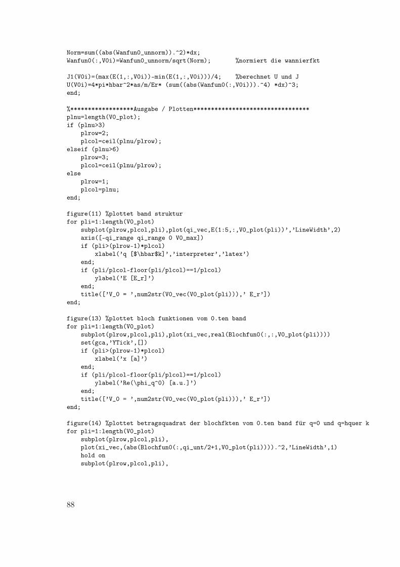
Norm=sum((abs(Wanfun0_unnorm)).^2)*dx;Wanfun0(:,V0i)=Wanfun0_unnorm/sqrt(Norm); %normiert die wannierfkt

J1(V0i)=(max(E(1,:,V0i))-min(E(1,:,V0i)))/4; %berechnet U und JU(V0i)=4*pi*hbar^2*as/m/Er* (sum((abs(Wanfun0(:,V0i))).^4) *dx)^3;end;

%******************Ausgabe / Plotten*********************************plnu=length(V0_plot);if (plnu>3)

plrow=2;plcol=ceil(plnu/plrow);

elseif (plnu>6)plrow=3;plcol=ceil(plnu/plrow);

elseplrow=1;plcol=plnu;

end;

figure(11) %plottet band strukturfor pli=1:length(V0_plot)

subplot(plrow,plcol,pli),plot(qi_vec,E(1:5,:,V0_plot(pli))’,’LineWidth’,2)axis([-qi_range qi_range 0 V0_max])if (pli>(plrow-1)*plcol)

xlabel(’q [$\hbar$k]’,’interpreter’,’latex’)end;if (pli/plcol-floor(pli/plcol)==1/plcol)

ylabel(’E [E_r]’)end;title([’V_0 = ’,num2str(V0_vec(V0_plot(pli))),’ E_r’])

end;

figure(13) %plottet bloch funktionen vom 0.ten bandfor pli=1:length(V0_plot)

subplot(plrow,plcol,pli),plot(xi_vec,real(Blochfun0(:,:,V0_plot(pli))))set(gca,’YTick’,[])if (pli>(plrow-1)*plcol)

xlabel(’x [a]’)end;if (pli/plcol-floor(pli/plcol)==1/plcol)

ylabel(’Re(\phi_q^0) [a.u.]’)end;title([’V_0 = ’,num2str(V0_vec(V0_plot(pli))),’ E_r’])

end;

figure(14) %plottet betragsquadrat der blochfkten vom 0.ten band für q=0 und q=hquer kfor pli=1:length(V0_plot)

subplot(plrow,plcol,pli),plot(xi_vec,(abs(Blochfun0(:,qi_unt/2+1,V0_plot(pli)))).^2,’LineWidth’,1)hold onsubplot(plrow,plcol,pli),

88

plot(xi_vec,(abs(Blochfun0(:,qi_unt+1,V0_plot(pli)))).^2,’--k’,’LineWidth’,1)hold offset(gca,’YTick’,[])if (pli>(plrow-1)*plcol)

xlabel(’x [a]’)end;if (pli/plcol-floor(pli/plcol)==1/plcol)

ylabel(’|\phi_q^0(x)|^2 [a.u.]’)end;title([’V_0 = ’,num2str(V0_vec(V0_plot(pli))),’ E_r’])

end;

figure(15) %plottet betragsquad. der wannierfkt des 0ten bandesfor pli=1:length(V0_plot)

hohe=max((abs(Wanfun0(:,V0_plot(length(V0_plot))))).^2 *dx);if (V0_vec(V0_plot(pli))==0) gitterhohe=0;else gitterhohe=hohe;end;subplot(plrow,plcol,pli),plot(xi_vec,(abs(Wanfun0(:,V0_plot(pli)))).^2 *dx,’LineWidth’,2)axis([-xi_range xi_range 0 hohe])hold onsubplot(plrow,plcol,pli),plot(xi_vec,gitter*gitterhohe,’r’)hold off%set(gca,’YTick’,[])if (pli>(plrow-1)*plcol)

xlabel(’x [a]’)end;if (pli/plcol-floor(pli/plcol)==1/plcol)

ylabel(’|w_0(x-x_0)|^2’)end;title([’V_0 = ’,num2str(V0_vec(V0_plot(pli))),’ E_r’])

end;

figure(16) %plottet tunnelwert Jplot(V0_vec,J1)xlabel(’lattice depth V0 [E_r]’)ylabel(’tunnel term J [E_r}’)title(’Tunnel Term J’)

figure(17) %plottet wechselwirkung Uplot(V0_vec,U)xlabel(’lattice depth V0 [E_r]’)ylabel(’interaction energy [E_r}’)title(’Onsite Interaction Energy’)

figure(18) %plottet die band -> plane wave decompositionfor pli=1:4

subplot(1,4,pli),bar(l_vec*2,(abs(c0n(:,pli))).^2)axis([-8 8 0 0.6])title([’Band n=’,num2str(pli-1)])if (pli==1) ylabel(’probability |a_{n,0}(l)|^2’)

89

end;%if (pli==2)text(2,-0.07,’plane wave with momentum $p=2l\hbar\,k$’,’interpreter’,’latex’)%end;xlabel(’2l’)

end;

figure(19) %plottet die plane wave -> band decompositionfor pli=1:4

subplot(1,4,pli),bar([0:10],(abs(c0n(l_tot+pli,:)’)).^2)axis([-1 8 0 0.6])title([’plane wave e^{i2lkx}, l=’,num2str(-1+pli)])if (pli==1) ylabel(’probability |a_{n,0}^*(l)|^2’)end;%if (pli==2) text(5,-0.07,’wavefunction $|n,0>$’,’interpreter’,’latex’)%end;xlabel(’n’)

end;

90

Bibliography

[AL03] H. Z. A. Liem, J. Limpert and A. Tünnermann, 100-W single-frequencymaster-oscillator fiber power amplifier, Opt. Lett. 28, 1537 (2003).

[Ami98] L. Amico and V. Penna, Dynamical Mean Field Theory of the Bose-Hubbard Model, Phys. Rev. Lett. 80, 2189 (1998).

[And95] M. H. Anderson, J. R. Ensher, M. R. Matthews, C. E. Wieman, and E. A.Cornell, Observation of Bose-Einstein Condensation in a Dilute AtomicVapor, Science 269, 198 (1995).

[And97] M. R. Andrews, C. G. Townsend, H.-J. Miesner, D. S. D. andD. M. Kurn,and W. Ketterle, Observation of Interference Between Two Bose-EinsteinCondensates, Science 275, 637 (1997).

[And98] B. P. Anderson and M. A. Kasevich, Macroscopic Quantum Interferencefrom Atomic Tunnel Arrays, Science 282, 1686 (1998).

[AS01] J. R. Abo-Shaeer, C. Raman, J. M. Vogels, and W. Ketterle, Observationof Vortex Lattices in Bose-Einstein Condensates, Science 292, 476 (2001).

[BD96] M. Ben Dahan, E. Peik, J. Reichel, Y. Castin, and C. Salomon, BlochOscillations of Atoms in an Optical Potential, Phys. Rev. Lett. 76, 4508(1996).

[Bes99] G. Best and O. M. Sezerman, Shedding light on hy-brid optics: A tutorial in coupling (1999), download:http://www.ozoptics.com/ALLNEW_PDF/ART0002.pdf.

[BIP98] BIPM, Le System Interational d’Unites (SI), Tech. rep., Bureau Interna-tional des Poids at Measures, Sevres, France (1998).

[Blo29] F. Bloch, Über die Quantenmechanik der Elektronen in Kristallgittern, Z.Physik 52, 555 (1929).

[Bos24] S. Bose, Plancks Gesetz und Lichtquantenhypothese, Z. Phys. 26, 178(1924).

[Bou82] M. Bouchiat, J. Guena, L. Hunter, and L. Pottier, Observation of a parityviolation in cesium, Physics Letters B 117, 358 (1982).

91

[Buc03] A. Buchleitner and A. R. Kolovsky, Interaction-Induced Decoherence ofAtomic Bloch Oscillations, Phys. Rev. Lett. 91, 253002 (2003).

[Car05] I. Carusotto, L. Pitaevskii, S. Stringari, G. Modugno, and M. Inguscio,Sensitive Measurement of Forces at the Micron Scale Using Bloch Oscil-lations of Ultracold Atoms, Physical Review Letters 95, 093202 (2005).

[Chi00] C. Chin, V. Vuletic, A. J. Kerman, and S. Chu, High Resolution FeshbachSpectroscopy of Cesium, Phys. Rev. Lett. 85, 2717 (2000).

[Chi01a] C. Chin, Cooling, Collisions and Coherence of Cold Cesium Atoms in aTrap, Ph.D. thesis, Stanford University (2001).

[Chi01b] C. Chin, V. Leiber, V. Vuletić, A. J.Kerman, and S. Chu, Measurementof an electron’s electric dipole moment using Cs atoms trapped in opticallattices, Phys. Rev. A 63, 33401 (2001).

[Chi04] C. Chin, V. Vuletic, A. J. Kerman, S. Chu, E. Tiesinga, P. Leo, and C. J.Williams, Precision Feshbach spectroscopy of ultracold Cs2, Phys. Rev. A70, 032701 (2004).

[Chi05] C. Chin, T. Kraemer, M. Mark, J. Herbig, P. Waldburger, H.-C.Nägerl,and R. Grimm, Observation of Feshbach-like resonances in collisions be-tween ultracoldmolecules, Phys. Rev. Lett. 94, 123201 (2005).

[Dal99] J. Dalibard, Collisional dynamics of ultra-cold atomic gases, in: M. In-guscio, S. Stringari, and C. E. Wieman (Eds.), Proceedings of the Inter-national School of Physics - Enrico Fermi, 321, IOS Press, 1999.

[Dav94] N. Davidson, H. Lee, M. Kasevich, and S. Chu, Raman Cooling of Atomsin Two and Three Dimensions, Phys. Rev. Lett. 72, 3158 (1994).

[Dav95] K. B. Davis, M.-O. Mewes, M. R. Andrews, N. J. van Druten, D. Durfee,D. M. Kurn, and W. Ketterle, Bose-Einstein Condensation in a Gas ofSodium Atoms, Phys. Rev. Lett. 75, 3969 (1995).

[Den00] J. Denschlag, J. E. Simsarian, D. L. Feder, C. W. C. andL. A. Collins,J. Cubizolles, L. Deng, E. W. Hagley, K. H. W. P. Reinhardt, S. L. Rol-ston, B. I. Schneider, and W. D. Phillips, Generating Solitons by PhaseEngineering of a Bose-Einstein Condensate, Science 287, 97 (2000).

[Den02] J. H. Denschlag, J. E. Simsarian, H. Häffner, C. McKenzie, A. Browaeys,D. Cho, K. Helmerson, S. L. Rolston, and W. D. Phillips, A Bose-Einsteincondensate in an optical lattice, Journal of Physics B 35, 3095 (2002).

[Ein25] A. Einstein, Quantentheorie des einatomigen idealen Gases. Zweite Ab-handlung, Sitzungber. Preuss. Akad. Wiss. 1925, 3 (1925).

92

[Els99] N. Elstner and H. Monien, Dynamics and Thermodynamics of the Bose-Hubbard model, Phys. Rev. B 59, 12184 (1999).

[Fis89] M. P. A. Fisher, P. B. Weichman, G. Grinstein, and D. S. Fisher, Bosonlocalization and the superfluid-insulator transition, Phys. Rev. B 40, 546(1989).

[Fli06] A. Flir, Implementierung und Untersuchung von Raman-Seitenbandkühlung zur Erzeugung eines ultrakalten Cäsium-gases, Master’s thesis, University of Innsbruck (2006), download:http://www.ultracold.at.

[Geh98] M. E. Gehm, K. M. O’Hara, T. A. Savard, and J. E. Thomas, Dynamicsof noise-induced heating in atom traps, Phys. Rev. A 58, 3914 (1998).

[Ger07] T. Gericke, F. Gerbier, A. Widera, S. Foelling, O. Mandel, and I. Bloch,Adiabatic loading of a Bose-Einstein condensate in a 3D optical lattice,Journal of Modern Optics 54, 735Ű743 (2007).

[Gre02a] M. Greiner, O. Mandel, T. Esslinger, and T. W. H. I. Bloch, Quantumphase transition from a superfluid to a Mott insulator in a gasof ultracoldatoms, Nature 415, 39 (2002).

[Gre02b] M. Greiner, O. Mandel, T. W. Hänsch, and I. Bloch, Collapse and revivalof the matter wave field of a Bose-Einstein condensate, Nature 419, 51(2002).

[Gre03] M. Greiner, Ultracold quantum gases in three-dimensional optical lat-tice potentials, Ph.D. thesis, Ludwig-Maximilians-Universität München(2003).

[Gri00] R. Grimm, M. Weidemüller, and Y. Ovchinnikov, Optical dipole traps forneutral atoms, Adv. At. Mol. Opt. Phys. 42, 95 (2000),

[Gui99] L. Guidoni and P. Verkerk, Optical lattices: cold atoms ordered by light,Journal of Optics B: Quantum and Semiclassical Optics 1, R23 (1999).

[Gup02] S. Gupta, K. Dieckmann, Z. Hadzibabic, and D. E. Pritchard, ContrastInterferometry using Bose-Einstein Condensates to Measure h/m and al-pha, Phys. Rev. Lett. 89, 140401 (2002).

[Hal] E. Haller, Phd thesis unpublished, university of Innsbruck.

[Hen00] J. Hensley, A. Whicht, B. Young, and S. Chu, Progress towards a Mea-surement of h/M, in: E. Arimondo, P. D. Natale, and M. Inguscio (Eds.),Proc. 17th Int. Conf. Atomic Physics, 43–57, AIP, Melville, New York,2000.

93

[Her03] J. Herbig, T. Kraemer, M. Mark, T. Weber, C. Chin, H.-C. Nägerl, andR. Grimm, Preparation of a Pure Molecular Quantum Gas, Science 301,1510 (2003), published online 21 Aug 2003, doi10.1126/science.1088876.

[Her05] J. Herbig, Quantum degenerate Cesium: Atoms and Molecules, Ph.D. the-sis, Innsbruck University (2005), download: http://www.ultracold.at.

[Ino98] S. Inouye, M. R. Andrews, J. Stenger, H.-J. Miesner, and D. M. S.-K. W.Ketterle, Observation of Feshbach resonances in a Bose-Einstein conden-sate, Nature 392, 151 (1998).

[Ino99] S. Inouye, T. Pfau, S. Gupta, A. P. Chikkatur, A. G. D. E. Pritchard,and W. Ketterle, Phase-coherent amplification of atomic matter waves,Nature 402, 641 (1999).

[Ise05] L. Isella and J. Ruostekoski, Nonadiabatic dynamics of a Bose-Einsteincondensate in an optical lattice, Physical Review A 72, 011601 (2005).

[Jak99] D. Jaksch, Bose-Einstein condensation and applications, Ph.D. thesis,University of Innsbruck (1999).

[Jul05] P. S. Julienne, C. J. Williams, Y. B. Band, and M. Trippenbach, LoadingBose-Einstein-condensed atoms into the ground state of an optical lattice,Physical Review A 72, 053615 (2005).

[Kam93] A. P. Kampf and G. T. Zimanyi, Superconductor-insulator phase transi-tion in the boson Hubbard model, Phys. Rev. B 47, 279 (1993).

[Kas02] V. A. Kashurnikov, N. V. Prokof’ev, and B. V. Svistunov, Revealing thesuperfluid–Mott-insulator transition in an optical lattice, Phys. Rev. A 66,031601 (2002).

[Ket99] W. Ketterle, D. S. Durfee, and D. M. Stamper-Kurn, Making, probing andunderstanding Bose-Einstein condensates, in: M. Inguscio, S. Stringari,and C. E. Wieman (Eds.), Proceedings of the International School ofPhysics - Enrico Fermi, 67, IOS Press, 1999, arxivcond-mat/9904034.

[Köh06] T. Köhler, K. Góral, and P. S. Julienne, Production of cold molecules viamagnetically tuneable Feshbach resonances, Reviews of Modern Physics78, 1311 (2006).

[Kit04] C. Kittel, Introduction to solid state physics, Wiley (8th ed), 2004.

[Kol04] A. R. Kolovsky, Bloch oscillations in the Mott-insulator regime, PhysicalReview A 70, 015604 (2004).

[Kra04] T. Kraemer, J. Herbig, M. Mark, T. Weber, C. Chin, H.-C. Nägerl, andR. Grimm, Optimized production of a cesium Bose-Einstein condensate,Appl. Phys. B 79, 1013 (2004).

94

[Kra06] T. Kraemer, M. Mark, P. Waldburger, J. Danzl, C. Chin, B. Engeser,A. Lange, K. Pilch, A. Jaakola, H.-C. Nägerl, and R. Grimm, Evidencefor Efimov quantum states in an ulracold gas of caesium atoms, Nature440, 315 (2006).

[Leo01] P. J. Leo, P. S. Julienne, F. H. Mies, and C. J. Williams, CollisionalFrequency Shifts in 133Cs Fountain Clocks, Phys. Rev. Lett. 86, 3743(2001).

[Mar07] M. Mark, T. Kraemer, P. Waldburger, J. Herbig, C. Chin, H. C. Naegerl,and R. Grimm, ‘St"uckelberg interferometry’ with ultracold molecules (2007).

[McK06] S. B. McKagan, D. L. Feder, and W. P. Reinhardt, An Investigation ofMean-field Effects for a Bose Condensate in an Optical Lattice, PhysicalReview A (Atomic, Molecular, and Optical Physics) 74, 013612 (2006).

[Met99] H. J. Metcalf and P. van der Straten, Laser cooling and trapping, Springer-Verlag, New York, 1999.

[Mey] T. P. Meyrath and F. Schreck, Digital RF Synthesizer: DC to135 MHz, Atom Optics Laboratory, University of Texas at Austin,http://george.ph.utexas.edu/ control/index.html, august 10, 2005 ed.

[New] Newport, Photonics Tutorial, www.newport.com.

[Orz01] C. Orzel, A. K. Tuchman, M. L. Fenselau, M. Yasuda, and M. A. Kasevich,Squeezed States in a Bose-Einstein Condensate, Science 291, 2386 (2001).

[Pet94] K. I. Petsas, A. B. Coates, and G. Grynberg, Crystallography of opticallattices, Phys. Rev. A 50, 5173 (1994).

[Pit03] L. Pitaevskii and S. Stringari, Bose-Einstein Condensation, InternationalSeries of Monographs on Physics 116, Oxford University Press, 2003.

[Reg03] C. A. Regal, C. Ticknor, J. L. Bohn, and D. S. Jin, Creation of ultracoldmolecules from a Fermi gas of atoms, Nature 424, 47 (2003).

[Ryc04] D. Rychtarik, B. Engeser, H.-C. Nägerl, and RudolfGrimm, Two-Dimensional Bose-Einstein Condensate in an Optical Surface Trap, Rhys.Rev. Lett. 92, 173003 (2004), doi10.1103/PhysRevLett.92.173003.

[Sch] F. Schreck, Manual of experiment control system CONTROL, Universityof Innbruck, http://george.ph.utexas.edu/ control/index.html, march 23,2003 ed.

95

[Sco04] R. G. Scott, A. M. Martin, S. Bujkiewicz, T. M. Fromhold, N. Malossi,O. Morsch, M. Cristiani, and E. Arimondo, Transport and disruptionof Bose-Einstein condensates in optical lattices, Physical Review A 69,033605 (2004).

[Sel04] J. Selim, Bose-Einstein Condensation of Molecules, Ph.D. thesis, Unver-sity of Innsbruck (2004), download: http://www.ultracold.at.

[SK98] D. M. Stamper-Kurn, H.-J. Miesner, A. P. Chikkatur, S. I. andJ. Stenger,and W. Ketterle, Reversible Formation of a Bose-Einstein Condensate,Phys. Rev. Lett. 81, 2194 (1998).

[Skl02a] S. E. Sklarz, I. Friedler, D. J. Tannor, Y. B. Band, and C. J. Williams,Flat-phase loading of a Bose-Einstein condensate into an optical lattice,Phys. Rev. A 66, 053620 (2002).

[Skl02b] S. E. Sklarz and D. J. Tannor, Loading a Bose-Einstein condensate ontoan optical lattice: An application of optimal control theory to the nonlinearSchrödinger equation, Phys. Rev. A 66, 053619 (2002).

[Sna98] M. J. Snadden, J. M. McGuirk, P. Bouyer, K. G. Haritos, andM. A.Kasevich, Measurement of the Earth’s Gravity Gradient with anAtom Interferometer-BasedGravity Gradiometer, Phys. Rev. Lett. 81, 971(1998).

[Sto05] M. Stoll and T. Köhler, Production of three-body Efimov molecules in anoptical lattice, Phys. Rev. A 72, 022714 (2005).

[TH04] H. J. K. T Hartmann, F Keck and S. Mossmann, Dynamics of Blochoscillations, New Journal of Physics 6, 2 (2004).

[Tha06] G. Thalhammer, K. Winkler, F. Lang, S. Schmid, R. Grimm, and J. H.Denschlag, Long-lived Feshbach molecules in a 3D optical lattice, Phys.Rev. Lett. 96, 050402 (2006).

[Tie92] E. Tiesinga, A. Moerdijk, B. J. Verhaar, and H. T. C. Stoof, Conditionsfor Bose-Einstein condensation in magnetically trapped atomic cesium,Phys. Rev. A 46, R1167 (1992).

[Unt05] P. Unterwaditzer, Aufbau eines vollständigen Diodenlasersystems zurLaserkühlung und Detektion von gespeicherten Cs-Atomen, Master’s the-sis, University of Innsbruck (2005), download: http://www.ultracold.at.

[Wan37] G. H. Wannier, The Structure of Electronic Excitation Levels in InsulatingCrystals, Phys. Rev. 52, 191 (1937).

96

[Web03a] T. Weber, Bose-Einstein Condensation of Optically Trapped Ce-sium, Ph.D. thesis, University of Innsbruck (2003), download:http://www.ultracold.at.

[Web03b] T. Weber, J. Herbig, M. Mark, H.-C. Nägerl, and R. Grimm, Bose-Einstein Condensation of Cesium, Science 299, 232 (2003).

[Web03c] T. Weber, J. Herbig, M. Mark, H.-C. Nägerl, and R. Grimm, Three-bodyrecombination at large scattering lengths in an ultracold atomicgas, Phys.Rev. Lett. 91, 123201 (2003), doi10.1103/PhysRevLett.91.123201.

[Win06] K. Winkler, G. Thalhammer, F. Lang, R. Grimm, J. H. Denschlag, A. J.Daley, A. Kantian, H. P. Buechler, and P. Zoller, Repulsively bound atompairs in an optical lattice, Nature 441, 853 (2006).

[Wit05] D. Witthaut, M. Werder, S. Mossmann, and H. J. Korsch, Bloch oscil-lations of Bose-Einstein condensates: Breakdown and revival, PhysicalReview E 71, 036625 (2005).

[Zen34] C. Zener, The Theory of the Change in Resistance in a Magnetic Field,Proceedings of the Royal Society of London. Series A 145, 268 (1934).

[Zwe03] W. Zwerger, Mott-Hubbard transition of cold atoms in optical lattices,Journal of Optics B 5, S9 (2003).

97

Danke

Nicht fehlen darf natürlich die Danksagung.Als erstes gebührt der Dank meinem Betreuer Hanns-Christoph Nägerl - denn

ohne ihn gäbe es diese Diplomarbeit nicht. Als höchst engagierter Forscher undProfessor schafft es Hanns-Christoph dennoch für allfällige Fragen immer zur Ver-fügung zu stehen.

Ich möchte auch Rudi Grimm dafür danken, mir eine Diplomarbeit in seinerArbeitsgruppe ermöglicht zu haben.

Ganz herzlich bedanken möchte ich mich bei Mattias und Elmar, quasi Pilot undCo-Pilot im CsIII Labor. Als Doktoranden waren sie es, die mein Unwissen undmeine Tollpatschigkeit ’auszubaden’ hatten. Besonders oft musste Elmar ’dranglauben’. Mit seiner ruhigen Art (muss wohl an Udo Jürgens liegen?) hat eres immer wieder geschafft, mir so manches ’geheimnisvolles’ Konzept näher zubringen. Danke Mattias, Danke Elmar.

Für einen gutes ’Laborklima’ mitverantwortlich war sicherlich auch ’Toni Su-perlegal’, dessen heitere Art immer wieder für gute Stimmung sorgte. Währendder Zeit des Verfassens war es auch ’El Boludo’, der meine Motivation mit seinementspannten Humor auf Kurs brachte. Gracias ca’on.

Ein grosses Danke auch dem Rest der Truppe, für die ausgesprochene Hilfs-bereitschaft bei technischen, physikalischen oder sonstigen Problemchen die mirim Zuge dieser Diplomarbeit so manches Kopfzerbrechen bereiteten, aber vorallemfür die kollegiale Atmosphäre.

In Bezug auf diese Arbeit möchte ich ausserdem Andrew, Orlaith und ’TheNiko-dude’ danken. Als ’native english-speakers’ haben Sie sich die qualvolle Mühegemacht Teile des Manuskripts korrekturzulesen.

99