a tutorial approach to the analysis of a geothermal ... · project number: mb8-aamx a tutorial...

Project Number: MB8-AAMX

A Tutorial Approach to the Analysis of aGeothermal Heating Problem

A Major Qualifying Project Report

submitted to the Faculty

of the

WORCESTER POLYTECHNIC INSTITUTE

in partial fulfillment of the requirements for the

Degree of Bachelor of Science

by

Eric Ostrom

Date: August 15, 2014

Approved:

Professor M. Berezovski, Advisor

Professor Arthur C. Heinricher, Advisor

1

Abstract

This report covers the background from calculus, ordinary differential equations, including

initial value problems and boundary value problems, that a student would need to use in

the analysis of a partial differential equation. The approach is used to complete a detailed

analysis of a mathematical model for a a geothermal heat pump.

Acknowledgments

I would like to thank Professor Tilley for his help with the geothermal sections as well

as Professors Berezovski and Heinricher for their help with the tutorial sections. I would

also like to thank my family, Lindsey Weber, Laura Rosen, and the staff in the Student

Development and Counseling Center for their support.

i

Contents

1 Introduction 1

1.1 Outline of the Report . . . . . . . . . . . . . . . . . . . . . . . . . . . . . . . 3

2 Key Tools from Calculus 6

2.1 Differential Calculus . . . . . . . . . . . . . . . . . . . . . . . . . . . . . . . 6

2.2 Integral Calculus . . . . . . . . . . . . . . . . . . . . . . . . . . . . . . . . . 8

2.2.1 Examples . . . . . . . . . . . . . . . . . . . . . . . . . . . . . . . . . 10

2.3 Basic Ordinary Differential Equations . . . . . . . . . . . . . . . . . . . . . . 12

3 Key Tools from Ordinary Differential Equations 13

3.1 First-order ODEs . . . . . . . . . . . . . . . . . . . . . . . . . . . . . . . . . 13

3.2 Qualitative Behavior of Solutions . . . . . . . . . . . . . . . . . . . . . . . . 16

3.3 Examples and Counter-Examples . . . . . . . . . . . . . . . . . . . . . . . . 18

3.4 Second Order ODEs . . . . . . . . . . . . . . . . . . . . . . . . . . . . . . . 21

3.4.1 Characteristic Equation . . . . . . . . . . . . . . . . . . . . . . . . . 21

3.4.2 Initial Conditions . . . . . . . . . . . . . . . . . . . . . . . . . . . . . 23

4 Boundary Value Problems 25

4.1 Boundary Conditions . . . . . . . . . . . . . . . . . . . . . . . . . . . . . . . 26

4.2 The most basic example . . . . . . . . . . . . . . . . . . . . . . . . . . . . . 26

5 Partial Differential Equations 28

5.1 Derivation of the Heat Equation . . . . . . . . . . . . . . . . . . . . . . . . . 28

5.2 Separation of Variables . . . . . . . . . . . . . . . . . . . . . . . . . . . . . . 29

ii

6 The Math and Physics of a Geothermal Heat Pump 33

7 Analysis of PDE for the Geothermal Heat Pump 42

7.1 Defining Parameters . . . . . . . . . . . . . . . . . . . . . . . . . . . . . . . 43

7.2 Nondimensionalization . . . . . . . . . . . . . . . . . . . . . . . . . . . . . . 44

7.3 Similarity Solution . . . . . . . . . . . . . . . . . . . . . . . . . . . . . . . . 45

7.4 Separation of Variables . . . . . . . . . . . . . . . . . . . . . . . . . . . . . . 45

7.5 Results . . . . . . . . . . . . . . . . . . . . . . . . . . . . . . . . . . . . . . . 48

8 Summary 54

A Matlab 55

iii

List of Figures

3.1 No Oscillation . . . . . . . . . . . . . . . . . . . . . . . . . . . . . . . . . . . 18

3.2 Blowing Up . . . . . . . . . . . . . . . . . . . . . . . . . . . . . . . . . . . . 19

3.3 Multiple solutions . . . . . . . . . . . . . . . . . . . . . . . . . . . . . . . . . 20

7.1 Pipe setup . . . . . . . . . . . . . . . . . . . . . . . . . . . . . . . . . . . . . 42

7.2 Varying Eigenvalues 1 . . . . . . . . . . . . . . . . . . . . . . . . . . . . . . 49

7.3 Varying Eigenvalues 2 . . . . . . . . . . . . . . . . . . . . . . . . . . . . . . 49

7.4 Varying Eigenfunctions 1 . . . . . . . . . . . . . . . . . . . . . . . . . . . . . 50




7.8 Temperature . . . . . . . . . . . . . . . . . . . . . . . . . . . . . . . . . . . . 52

iv

List of Tables

7.1 Parameters . . . . . . . . . . . . . . . . . . . . . . . . . . . . . . . . . . . . 43

v

Chapter 1

Introduction

The purpose of this project is to develop and explain the mathematical background that an

undergraduate student would need to attack an applied mathematics problem involving par-

tial differential equations. The application is from geothermal heating and the mathematical

tools include calculus, ordinary differential equations, and partial differential equations.

The mathematical model for heat flow in a uniform bar illustrates the basic tools that

we will review in this report. Picture a metal bar of length L where the goal is to model the

temperature for the bar at each position x between x = 0 and x = L and each time t ≥ 0.

Let u = u(x, t) be the function that records the temperature we are modeling. With a little

bit of basic physics, (see Lesson 4 of [10] or the summary on page 28 in this report) we arrive

at the heat equation:

ut = uxx (1.1)

In this equation,

ut =∂u

∂t

is the rate of change of temperature with respect to time t for a fixed x and

uxx =∂2u

∂x2

is the “concavity” of u with respect to x for fixed t. There is usually added information,

such as the requirement that the temperatures at the endpoints x = 0 and x = L are fixed

for all time:

u(0, t) = u0, and u(L, t) = uL for all t ≥ 0. (1.2)

1

There could also be a specified initial temperature profile:

u(x, 0) = φ0(x) for 0 < x < L. (1.3)

Basically, the partial differential equation (1.1) says that the temperature at a point is

changing rapidly (in time for that fixed x) if the temperature u is very convex or concave

at the point x. On the other hand, if the slope of u (in the x-direction) is constant, then

uxx = 0 and the temperature is constant (again, in time for the fixed x).

In some applications, boundary conditions have a different physical meaning. For exam-

ple, requiring that

ux(0, t) = 0, and ux(L, t) = 0 for all t ≥ 0 (1.4)

means that there is no heat flow through the boundary (the boundary is insulated from the

surrounding material). Boundary conditions such as

ux(0, t) + u(0, t) = 0, and ux(L, t) + u(L, t) = 0 for all t ≥ 0 (1.5)

are an application of the basic Newton Law of Cooling at the boundary where the heat flow

depends on the temperature at the boundary. For example, the temperature will decrease

in the x-direction (ux(0, t) < 0) if the temperature at the boundary (or just outside the

boundary) is positive (u(0, t) > 0 so that ux(0, t) = −u(0, t) < 0).

We will consider at least three different methods for solving equation (1.1) in later chap-

ters, but it is instructive for this introduction to consider one of the simplest. This approach

is called the method of similarity solutions1 and the basic idea is to look for solutions of a

particular form:

u = u(x, t) = f(x/√t)

= f(y) where y := x/√t.

In words, the solution in the (x, t) plane is constant along curves of the form x = const ·√t.

We plug these into the heat equation (1.1) to obtain

uxx =∂2u

∂x2= f ′′(y) · 1

t

1There is a nice video created by Professor Chris Tisdell explaining the method at

https://www.youtube.com/watch?v=dNLmvhZWEq8.

2

ut =∂u

∂t= f ′(y) · x√

t3· −1

2=−1

2f ′(y) · y · 1

t

. So, rearranging terms,

f ′′(y) + f ′(y)y

2= 0. (1.6)

The good news is that the original partial differential equation (1.1) has been transformed

into an ordinary differential equation (1.6).

The better news is that this new ordinary differential equation can be solved (by sepa-

rating and integrating):

f(y) = −C∫ ∞y

e−s2/4ds.

We have then

u(x, t) = f(x/√t)

= −C∫ ∞x/√t

e−s2/4ds. (1.7)

Not a really nice formula for the solution, but a solution and a formula none the less. The

reader may be, and probably should be, a little nervous that the formula in (1.7) has a bit

of a problem at t = 0 because we are dividing by√t:

u(x, 0)?= −C

∫ ∞∞

e−s2/4ds.

It isn’t at all clear what this last integral means and should, at least, be interpreted carefully

as a limit. It is also not clear how the initial and boundary conditions can be satisfied by

this special solution.

1.1 Outline of the Report

This report is intended to be a tour of the mathematical tools from Calculus and Ordinary

Differential Equations that student would need to understand in order to analyze a pretty

complex partial differential equation that arises in a realistic application.

In the next chapter, we are going to start with the basic tools that a WPI student would

learn to use in Calculus. The main point here is that the problems solved in Calculus II

(evaluating integrals and finding antiderivatives) are key to solving what are called ordinary

differential equations.

3

The theory of ordinary differential equations is reviewed in Chapter 3. The material

discussed here includes some of the basic theory of existence and uniqueness for solutions as

well as the qualitative behavior of solutions. The theory tells us when it is worth looking

for a solution (one will exist) and when the solution we find is the only possible solution (we

have uniqueness).

The basic tools from Calculus (simple integration) don’t quite cover the kinds of problems

that arise when the equations involve both first and second derivatives. In many cases, the

second-order equation can be transformed to a system of first-order equations and so the

fundamental existence and uniqueness theorems apply. In some cases, it is possible to reduce

the second-order differential equation to a first-order equation and to use the basic calculus

tools to actually solve the problem.

When solving a differential equation, we usually find a “general solution” first and then

are faced with the challenge of choosing the one solution that fits the physical problem. For

example, in using Newtonian mechanics, if a particle moves on a line with position x = x(t)

at time t, the analysis starts with F = ma = mx. If there is no force acting on the particle,

then F = 0 and so x = 0. Just integrate twice to find that x(t) = C1 + C2t. This is the

“general solution” but there is exactly one solution with a specified position and velocity at

some fixed time. In fact, in this solution, C1 is the position at time t = 0 and C2 is the

velocity at time t = 0 (and in fact the velocity for any time t!).

Notice that we need two pieces of information to find a unique solution to a second-order

differential equation. For third-order differential equations, we would need three pieces of

data. For initial value problems (IVP), all of the data are given at one specific time or

position. In some applications, the two pieces of information could tell us something about

the solution at two different times or places. These types of problems are called boundary

value problem (BVP) and bring a new set of challenges to the solution process.

The bad news is that we lose some of the nice uniqueness theory when we move from

initial value problems to boundary value problems. This is in fact good news for applications

like the geothermal heat pump model (and the heat equation) because this non-uniqueness

provides the flexibility needed to build the solutions we need. In the cases studied here, zero

is always a solution but the BVP can also have non-zero solutions, called eigenfunctions, and

4

we can use these eigenfunctions to build solutions to complex problems. The eigenfunctions

are associated with eigenvalues which are parameters that appear when we use the method

of separation of variables to turn the PDE into a family of ODE’s. We will go over what an

eigenfunction and an eigenvalue are in Section 4.2.

In a partial differential equation (PDE), the unknown function has more than one variable

and rates of change depend on directions. The methods used to solve ODEs don’t work

immediately on PDEs because the answers we get will get depend on the “direction” we

integrate. However, one common method for solving a PDE is to turn it into a family of

ODEs, then we can use methods for solving ODEs on each member of the family. The most

common way to do this is called separation of variables.

Partial differential equations arise when we analyze a geothermal heat pump system.

Geothermal heat pump systems have been developed to use the ground as a heat source (or

sink) for heating (or cooling) buildings. Mathematically, a geothermal system uses the heat

equation, a PDE. We will look more deeply at this example in Chapters 6 and 7.

5

Chapter 2

Key Tools from Calculus

This chapter starts with the assumption that the reader is a first or second-year student

(probably at WPI) who has a basic background in calculus (integral and differential). The

goal is to review the key topics and ideas that are necessary for the analysis of the physical

system summarized in Chapter 7 on geothermal heating.

A differential equation is an equation that involves an unknown function (say y), its

derivatives (such as y′ or y′′), and its independent variable (say x). For example, y′(x) = x

is differential equation for the unknown function y = y(x) which can be solved by simply

integrating both sides with respect to x. If we change the problem slightly to y′(x) = y,

we still have a differential equation for the unknown function y = y(x) but cannot simply

“integrate both sides” with respect to x; the problem is that the unknown function y now

appears on both sides of the equation. It turns out that we can still use the basic tools of

calculus to solve this differential equation, but we need to do some rearranging first; we need

to separate variables before we can integrate.

Before we begin looking at differential equations, we need to review the relevant topics

of Calculus. The relevant topics include derivatives, antiderivatives, and integrals.

2.1 Differential Calculus

Calculus classes can be summarized in the following way: define the derivative and then

develop the rules that let us calculate the derivative for more and more complex functions.

6

Along the way, connect the calculations to applications from engineering and science. The

most basic physical example asks that we find the velocity (or acceleration) for a particle if

we know the position at each time t. The basic approach is to compute an average velocity:

x(t+ ∆t)− x(t)

∆t=

∆x

∆t

is the average velocity on the interval [t, t+ ∆t]. If we take a limit as ∆t→ 0 we obtain an

instantaneous velocity.

To make this a little more concrete, the derivative of a function f of a single variable x

is defined by the limit:

f ′(x) := lim∆x→0

f(x+ ∆x)− f(x)

∆x(2.1)

If we think of the graph of the function f(x) in the (x, y)-plane, then f ′(x) is the slope of

the tangent line to the curve at the point (x, f(x)). For the definition of the derivative, see

page 99 in[20].

For example, if the function is f(x) = x2, then we can compute the limit in (2.1):

lim∆x→0

(x+ ∆x)2 − x2

∆x= lim

∆x→0

x2 + 2x∆x+ ∆x2 − x2

∆x= lim

∆x→02x+ ∆x = 2x.

It isn’t hard to show that the same basic argument works for any power n:

lim∆x→0

(x+ ∆x)n − xn

∆x= lim

∆x→0

xn + nxn−1∆x+ · · ·+ ∆xn − xn

∆x

= lim∆x→0

nxn−1 +O(∆x)

= nxn−1 (Wahoo!)

We have then the general power rule:

d

dxxn = nxn−1 (2.2)

While the calculations above seem to assume that n was a positive integer, this rule in fact

works for any real number n.

Perhaps the most useful theorem from Differential Calculus is the so-called Chain Rule.

It allows us to compute the derivative for more and more complex functions by treating them

7

a compositions of simpler functions. The Chain Rule says that the derivative of f composed

with g is the product of the derivatives:

d

dxf(g(x)) = f ′

(g(x)

)· g′(x) (2.3)

where it is important to note that the prime (′) must be interpreted carefully. Here is an

example.

Example 2.1. Define f(x) := sin(x) and g(x) := 2πx. Then

f ′(x) = cos(x) and g′(x) = 2π

and the Chain Rule tells us that

d

dxsin(2πx) = cos(2πx) · 2π

There is one more definition from Calculus that is crucial to the discussion of the geother-

mal heat pump: the partial derivative. When a function depends on more than one variable,

then there is more than one direction to use when computing the derivative. (Picture a hill:

the slope depends on the direction you walk.) The definition for a partial derivative takes

the basic definition and uses it for each variable separately:

ux(x, t) := lim∆x→0

u(x+ ∆x, t)− u(x, t)

∆x(2.4)

ut(x, t) := lim∆t→0

u(x, t+ ∆t)− u(x, t)

∆t(2.5)

All of the Calculus rules that work for functions of one variable apply again.

2.2 Integral Calculus

The next step in Calculus reverses the question: if we know the derivative of a function, can

we find the function? Again, the most basic physical example asks us to find the position

of a particle at time t if we know the velocity at all times t. It turns out that this physical

problem is closely tied to the problem of finding the area under or between curves. This is

8

the connection between the integral defined by the Riemann sum and the antiderivative and

the connection is captured in the Fundamental Theorem of Calculus.

We call F (x) an antiderivative for f(x) if F ′(x) = f(x). Note that we did not say the

antiderivative; if we can find one, then adding a constant gives us another antiderivative. For

example, we know from Calculus I (and the example just completed) that one antiderivative

for 2x is x2 (because the derivative of x2 is 2x). We also know that another antiderivative

is x2 + 2π because the derivative of the added constant is zero. To see the definition of the

antiderivative, see page 248 of [20].

Finding the antiderivative usually relies on knowledge of many basic derivatives and a few

rules (like the chain rule) that reduce complicated problems to simpler ones. For example,

if f(x) = 2x then the last example demonstrated that F (x) = x2 is an antiderivative for

f(x). To simplify notation, and perhaps to confuse many generations of students, a standard

notation for the antiderivative is ∫f(x)dx = F (x).

This is called the integral sign and it just happens to be the same symbol used to define

another mathematical object, called the Riemann integral.

The Riemann integral is defined as the limit of Riemann sums:∫ b

a

f(x)dx := limN→∞

N∑j=1

f(xj)b− aN

(2.6)

where

xj = a+ j · b− aN

, j = 1, . . . N.

If we think of the graph of y = f(x) in the (x, y)-plane, then the summation on the right

is an approximation to the area between the curve and the x-axis (we are adding a bunch

of rectangles with width (b− a)/N and height f(xj)). In the limit as N goes to infinity, we

get the area under the curve. To be precise, we should call (2.6) a Riemann integral. Note

that the actual definition is more general and allows non-uniform mesh and evaluation at

different points, but this is the basic idea. To see the definitions of the Riemann Sum and

the definite integral, see pages 272-273 of [20].

The Fundamental Theorem of Calculus makes the connection between the antiderivative

and the Riemann integral:

9

Theorem 2.1. Given a function f(x) continuous on the interval a ≤ x ≤ b. If F (x) is an

(any) antiderivative for f(x), then∫ b

a

f(x)dx = F (b)− F (a).

To see a proof of the Fundamental Theorem of Calculus, see page 282 in [20]. The basic

idea is that if you define a function by the Riemann integral with a variable upper limit:

G(x) :=

∫ x

a

f(z)dz

you can show (pretty easily) that G(x) is an antiderivative.

2.2.1 Examples

Now we will work our way through three examples that a student might see in a Calculus II

course.

Example 2.2. Find the antiderivative for f(x) = x3.

The power rule for the derivative (equation (2.2)) can be turned around to provide a

power rule for integration: the antiderivative of xn is 1n+1

xn+1. So we have∫x3dx =

1

4x4 + C (2.7)

Notice that there is an arbitrary constant C. This means that there is a family of solutions

that depend on C that are all antiderivatives.

If we were asked to compute an integral, then using the Fundamental Theorem of Cal-

culus, we get ∫ 10

0

x3dx =1

4x4∣∣10

0=

104

4− 04

4= 2500 (2.8)

Example 2.3. Find the following antiderivative:∫2x cos(x2)dx (2.9)

10

In this example, u = x2 and du = 2x dx. Thus∫2x cos(x2)dx =

∫cos(u)du = sin(u) + C = sin(x2) + C (2.10)

This method, called u-substitution in Calculus II, is just the Chain Rule from Calculus I

(backwards).

Example 2.4. ∫ x

1

1

udu (2.11)

Notice that the problem has limits but one of the limits is a variable. This means that the

end result will be an equation. Therefore,∫ x

1

1

udu = ln(u)

x

1 = ln(x)− ln(1) = ln(x) (2.12)

It is important to realize the difference between the x and the u. Although we are integrating

with respect to u, the solution is a function of x.

11

2.3 Basic Ordinary Differential Equations

The difference between a differential equation and a simple integration problem is merely

the way it is worded. Some differential equations can be rewritten as a simple integration

problem, but some are more complicated. This does not mean that they cannot be solved,

but that they are a different type of problem and require a little bit of ingenuity.

All of the integration problems discussed in the last section can be rewritten as differential

equation. For example, the problem solved in Example 2.2 can be restated as solve

dy

dx= x3, y(0) = 0

and then find y(10) = 2500.

Equation (2.9) can be restated as solve

dy

dx= 2x cos(x2).

Equation (2.11) can be rewritten as

dy

dx=

1

x, y(1) = 0.

Another simple example of a differential equation is y′ = y whose solution is y = Cex.

This may look likedy

dx= x

but it is fundamentally different. We cannot just “integrate both sides” because that would

ask us to compute∫ydx and we don’t y(x) yet. We can do some algebra and rewrite

the differential equation so that the unknown function does not appear on one side of the

equation and then we can just integrate. The real solution is∫dy

y=

∫dx⇒ ln(y) = x+ C ⇒ y = ex+C = C1e

x

We’ll look at this type of problem again when we discuss characteristic equations in

Section 3.4.1.

12

Chapter 3

Key Tools from Ordinary Differential

Equations

There are many different types of ordinary differential equations (ODEs). The term “ordi-

nary” just means that there are only ordinary derivatives and there is only one independent

variable. We start with the simplest kind of first-order ordinary differential equation where

it is possible to build a solution by integration. Second-order differential equations require a

different approach and we’ll consider only the simple case of constant coefficients where the

method of characteristic equations works. The ordinary differential equation almost always

has an infinite family of solutions where a single unique solution is obtained when initial

data (like position and velocity at time t = 0) is added to the problem specification.

3.1 First-order ODEs

How do we solve

y′(x) = F (x, y(x)), y(x0) = y0? (3.1)

Before we look into solving this problem, we need to know if there exists a unique solution.

Theorem 3.1. Given equation (3.1), if F and Fy are continuous near (x0, y0), then there

exists a unique solution near the point.

To see the theorem, see page 4 in [11]. In [7], see page 125 for the Uniqueness theorem

13

and page 128 for the Existence theorem or page 130 to see a Corollary that looks like this

theorem.

Uniqueness proof:

Assume that we have two solutions, u(x) and v(x) for equation (3.1). We must show

u(x) ≡ v(x), x0 ≤ x ≤ x1. Let’s assume there is some interval a < x < b, x0 ≤ a < b ≤ x1

where u 6= v while u(a) = v(a). We can assume that w(x) = u(x) − v(x) > 0 on the open

interval a < x < b. (If not, then we have w(x) = 0 for all x and so so u(x) ≡ v(x) and the

theorem is proved.) Therefore

w′(x) = F (x, u(x))− F (x, v(x))

by applying Taylor’s theorem to the second argument of F , we have

w′(x) = F (x, u(x))− F (x, v(x)) =∂F (x, ξ)

∂yw(x)

where ξ is between u(x) and v(x). The choice of ξ depends on x, but the continuous function

|∂F (x, ξ)/∂y| is bounded by a constant M and so

w′(x) ≤M |w(x)| for all x0 ≤ x ≤ x1.

But |w(x)| = w(x) for a < x < b and

w′ ≤Mw, a ≤ x < b

Now multiply by e−Mx. This turns w′−Mw ≤ 0 into (we−Mx)′ ≤ 0. Integrating from x = a

gives us

w(x)e−Mx − w(a)e−Ma ≤ 0

Since w(a) = u(a)− v(a) = 0,

w(x)e−Mx ≤ 0

forcing w(x) ≤ 0 which contradicts w(x) > 0. Therefore w(x) = u(x)− v(x) ≡ 0.

Existance proof: For some a, b > 0, the domain within which F is defined includes the

rectangle

R = {(x, y) : |x− x0| ≤ a, |y − y0| ≤ b}

14

Let M represent the maximum value of |F (x, y)| on R and L represent the maximum value

of |∂F (x, y)/∂y| on R. Next we will construct a sequence of approximations. Since F is

defined in a neighborhood of (x0, y0), f(s, y0) is defined provided |s− x0| ≤ a. Hence

y1(x) = y0 +

∫ x

x0

f(s, y0)ds

is defined for |x − x0| ≤ a. To calculate the next iterate requires that F (s, y1) be defined.

Therefore, we must guarantee that |s − x0| ≤ a and |y1(s) − y0| ≤ b remain in R. Since

|f | ≤M on R,

|y1(s)− y0| =∣∣∣∣∫ x

x0

F (s, y0)ds

∣∣∣∣ ≤ ∫ x

x0

|F (s, y0)|ds ≤M(x− x0)

To keep (x, y1(x)) in R, we must further restrict x so that Mx ≤ b; therefore, we demand

|x− x0| ≤ min(a, b/M). This argument applies to each of the iterates yn(x).

To examine the convergence of the iterates, restrict x further by requiring |x − x0| ≤min(a, b/M, α/L) for some α < 1. Also, if y(x), z(x) are any two functions defined for such

values of x, let

||y − z|| = max{|y(x)− z(x)| : |x− x0| ≤ min(a, b/M, α/L)}

We will use ||...|| to compare the maximum distance between iterates.

To compare ym(x) and yn(x) for arbitrary iterates m,n, compute

|ym(x)− yn(x)| =∣∣∣∣∫ x

x0

[F (s, ym−1(s))− F (s, yn−1(s))]ds

∣∣∣∣≤∫ x

x0

|F (s, ym−1(s))− F (s, yn−1(s))|ds

≤∫ x

x0

max(s,y)∈R

[∣∣∣∣∂F∂y (s, y)

∣∣∣∣] |ym−1(s)− yn−1(s)|ds

≤ L

∫ x

x0

|ym−1(s)− yn−1(s)|ds

≤ L(x− x0)||ym−1 − yn−1||

Since L|x− x0| ≤ α, this string of inequalities yields

||ym − yn|| ≤ α||ym−1 − yn−1||

15

If m > n, then

||ym − yn|| ≤ α||ym−1 − yn−1|| ≤ α2||ym−2 − yn−2|| ≤ ... ≤ αn||ym−n − y0||

Using triangle inequality and contraction relation, we obtain

||ym−n − y0|| = ||ym−n − ym−n−1 + ...+ y2 − y1 + y1 − y0||

≤ ||ym−n − ym−n−1||+ ...+ ||y2 − y1||+ ||y1 − y0||

≤ (αm−n−1 + ...+ α + 1)||y1 − y0||

≤ b

1− α

Combining the results, we get

||ym − yn|| ≤αnb

1− α, m ≥ n

Since α < 1, as n (and m) grows large, the sequence converges. Therefore, y(x) =

limn→∞ yn(x) and we have constructed a solution to the initial value problem.

3.2 Qualitative Behavior of Solutions

One of the important lessons that students learn in studying differential equations is that

finding “the solution” isn’t always the goal. In particular, the differential equation itself

sometimes contains more information about the behavior of the solution than the solution

formula itself. For example, if we have the equation y′ = y2 then we know that the solution

curve is nondecreasing simply because the righthand side of the equation is always greater

than or equal to zero.

Example 3.1. Solutions cannot oscillate.

Start with a really simple ODE

y′ = F (y), y(x0) = y0. (3.2)

The claim is that any solution to this equation must be increasing all of the time or decreas-

ing all of the time (or constant). The solutions cannot oscillate.

16

A student probably knows how to solve some even simpler examples. For example, the

solution to

y′(x) = cos(x), y(0) = 0 (3.3)

is (just by integrating both sides)

y(x) = sin(x).

What is special about equation (3.2) (and not true about (3.3)) is that the righthand

side of the differential equation depends on the solution y but not the independent variable x.

Before looking at the example more carefully, try to find an example of an equation like

(3.2) which does oscillate. An obvious first try would be

y′ =√

1− y2, y(0) = 0. (3.4)

Separate and integrate:

dy√1− y2

= dx ⇒∫

dy√1− y2

=

∫dx (3.5)

The result is

arcsin(y) = x+ C

and using the initial condition, we get C = 0 so the solution is y = sin(x). The problem is

that the step where we inverted the sine function assumed that the domain was limited to

an interval (like −π/2 ≤ x ≤ π/2) on which the sine curve is actually monotone increasing.

In other words, we don’t get the full sin(x) curve as a solution, only a small segment that

does not oscillate.

Now go back to the original example. Assume that we have a solution curve that does

actually oscillate. What that means is that we can find a horizontal line y = y1 and the

solution curve must cross that line going up at some position x1 (so the slope is positive at

x1). There has to be a later position x2 where the solution curve crosses again, but now

going down so the slope at x2 is negative. But then we have the following:

0 < y′(x1) = F (y(x1)) = F (y1) = F (y(x2)) = y′(x2) < 0

and the inequalities at each end of the sandwich are strict. This is a contradiction and shows

that the solution curve cannot oscillate.

17

Figure 3.1: No Oscillation

3.3 Examples and Counter-Examples

Example 3.2. No Solutions.

y′ = F (y), y(x0) = y0. (3.6)

The claim is that there may be no solution to this . Let’s start with a simple example.

y′ =

−10 : x ≥ 0

10 : x < 0

with the initial condition y(0) = 0. Because F (y) is discontinuous at y = 0, the existence

theorem is broken. Besides, where would we go? As soon as we try to leave zero, we are

forced back up.

Example 3.3. Solutions can blow-up in finite time.


y′ = F (y), y(x0) = y0. (3.7)

The claim is that any solution to this equation can go to infinity before the independent

variable reaches infinity.

Let’s start with a simple example.

y′ = y2, y(0) = 1 (3.8)

18

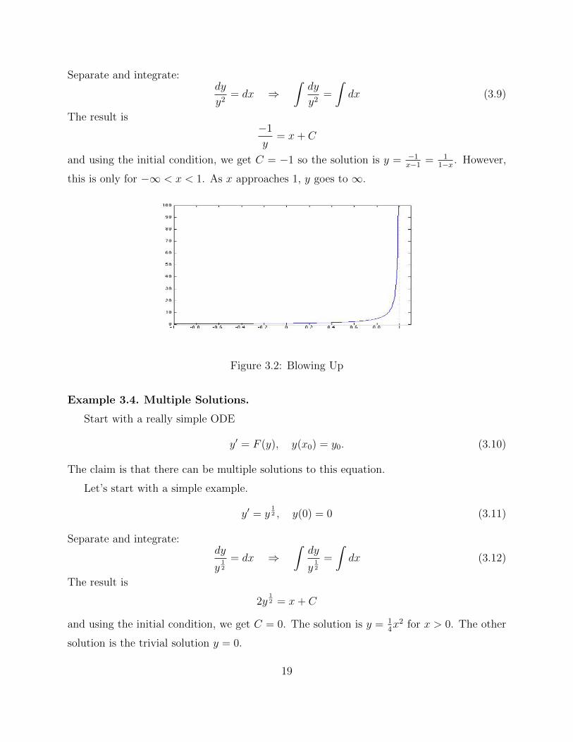
Separate and integrate:dy

y2= dx ⇒

∫dy

y2=

∫dx (3.9)

The result is−1

y= x+ C

and using the initial condition, we get C = −1 so the solution is y = −1x−1

= 11−x . However,

this is only for −∞ < x < 1. As x approaches 1, y goes to ∞.

Figure 3.2: Blowing Up

Example 3.4. Multiple Solutions.


y′ = F (y), y(x0) = y0. (3.10)

The claim is that there can be multiple solutions to this equation.

Let’s start with a simple example.

y′ = y12 , y(0) = 0 (3.11)

Separate and integrate:dy

y12

= dx ⇒∫

dy

y12

=

∫dx (3.12)

The result is

2y12 = x+ C

and using the initial condition, we get C = 0. The solution is y = 14x2 for x > 0. The other

solution is the trivial solution y = 0.

19

Figure 3.3: Multiple solutions

20

3.4 Second Order ODEs

Previously we worked with first order ODEs. This means that the highest derivative is one.

Now we will work with second order ODEs with second derivatives. Old solution methods

do not work anymore. For example, for y′ = y we can separate and integrate. However, for

y′′ = y we cannot separate and integrate.

d2y

dx2= y ⇒ d(y′)

y= dx

but y cannot be integrated with respect to y′.

To show why this is true, let us assume that y = x2

dy′

y?=d(2x)

x2= 2

dx

x26= dy

y

3.4.1 Characteristic Equation

If the equation is of the form

ay′′ + by′ + cy = 0 (3.13)

with constant coefficients. Then we will assume the solutions are of the form

y = erx

Once we plug this in, we get

ar2erx + brerx + cerx = 0

We can factor out the exponential.

erx(ar2 + br + c) = 0

Since the exponential can never equal zero, we need to find the roots of the characteristic

equation

ar2 + br + c = 0. (3.14)

If there are two distinct real roots r1, r2 then the solution is of the form

y = C1er1x + C2e

r2x (3.15)

21

If there is one repeated real root r then the solution seems to be

y = C1erx + C2e

rx = (C1 + C2)erx (3.16)

so there is only one constant. There is in fact a distinct solution but it does not come directly

from the characteristic equation. To find this solution, look for a new solution of the form

y(x) = u(x)erx. Plug this in and collect terms to find that u(x) must satisfy u′′ = 0, which

implies that u(x) = x and so the general solution when the characteristic equation has a

repeated root is

y = C1erx + C2xe

rx (3.17)

If the roots are complex r = a± bi then the solution is of the form

y = C1eax sin(bx) + C2e

ax cos(bx) (3.18)

where we used Euler’s equation

eiθ = cos(θ) + i sin(θ)

Example 3.5. Let us solve

y′′ + 3y′ − 4y = 0 (3.19)

If we use a characteristic equation, we get r2 + 3r − 4 = 0 which can be factored to (r +

4)(r − 1) = 0. Thus r1 = −4 and r2 = 1. Therefore, the solution is

y = C1e−4x + C2e

x


y′′ + 2y′ + 1y = 0 (3.20)

If we use a characteristic equation, we get r2 + 2r + 1 = 0 which can be factored to (r +

1)(r + 1) = 0. Thus r1 = r2 = −1. Therefore, the solution is

y = C1e−x + C2xe

−x


y′′ + y = 0 (3.21)

22

If we use a characteristic equation, we get r2 + 1 = 0 which cannot be factored. However,

r2 = −1. Thus r = ±i. Therefore, the solution is

y = C1 sin(x) + C2 cos(x)

Example 3.8. Solve

y′′ = 0 (3.22)

For this problem, we just integrate to get

y = C1 + C2x

But we get the same solution by using the characteristic equation method. The characteristic

equation is r2 = 0. Thus r1 = r2 = 0. So

y = C1e0 + C2xe

0 = C1 + C2x

Example 3.9. Now if the coefficients are not constant, such as in

y′′ + xy = 0 (3.23)

then this method will not work. If we assume the solution is

y = erx

and we are assuming that r is constant, then we can plug in and get

0 = r2erx + xerx (3.24)

= (r2 + x)erx (3.25)

Since the exponential is never zero, r2 + x = 0. But this cannot be true for all x if r is

constant.

3.4.2 Initial Conditions

A second order ODE needs two initial conditions. These initial conditions are often at the

same point:

y(x0) = y1, y′(x0) = y2

23

The reason that we need two initial conditions is because in a second order ODE, there are

two constants of integration. These conditions allow us to solve for the constants and get a

unique solution.

Example 3.10. Look at example 3.5 with initial conditions y(0) = 1, y′(0) = 6.

y(x) = C1e−4x + C2e

x

Then plug in and get

y(0) = C1e0 + C2e

0 = C1 + C2 = 1 (3.26)

The derivative is

y′(x) = −4C1e−4x + C2e

x

and plug in to get

y′(0) = −4C1e0 + C2e

0 = −4C1 + C2 = 6 (3.27)

now subtract equation (3.27) from (3.26). The result is

5C1 = −5⇒ C1 = −1

Therefore

−1 + C2 = 1⇒ C2 = 2

Thus the solution is

y(x) = −e−4x + 2ex

24

Chapter 4

Boundary Value Problems

One difference between an initial value problem (IVP) and a boundary value problem (BVP)

is that the conditions for the BVP are separated in time or space.

Example 4.1. The IVP

y′′ + y = 0, y(0) = 0, y′(0) = 1

has exactly one solution y = sin(x). Although

y′′ + y = 0, y(0) = 0, y(π

2

)= 1

has the same solution of y = sin(x), it is a different type of problem. To show that it has the

same solution, notice that the solution is of the form y = C1 sin(x) +C2 cos(x). By applying

the first boundary condition, we have C2 = 0. By applying the second boundary condition,

we have C1 = 1. Therefore the solution is y = sin(x).

However, there are BVPs that have infinitely many solutions.

Example 4.2. Look at

y′′ + y = 0, y(0) = 0, y(π) = 0

Notice that the solution is of the form y = C1 sin(x) + C2 cos(x). By applying the first

boundary condition, we have C2 = 0. By applying the second boundary condition does

not give us a value for C1. Therefore the solution is y = C sin(x) for any real number C.

Therefore, there are infinitely many solutions.

25

4.1 Boundary Conditions

The boundary conditions do not need to be positions at two points. It can have derivatives

at points like

y′′ + y = 0, y′(0) = 1, y′(π

2

)= 0

with solution y = sin(x). However, there can be a combination as well, such as

y′′ + y = 0, y(0) = 0, y′(π

2

)+ y

(π2

)= 1

with solution y = sin(x).

4.2 The most basic example

In linear algebra a student learns about eigenvalues and eigenvectors. Take a set of linear

equations in matrix form: A~x = λ~x. Here A is a square matrix, ~x is a vector, and λ is a

constant. Notice that ~x = 0 is always a solution. For a given matrix A, there may exist

λs, called eigenvalues, where we can find a nonzero solutions ~x, called the eigenvectors. The

eigenvalues and eigenvectors are paired so that the equation is only true when both are

plugged in. See page 76 in [11].

Let us look at how we find eigenvalues. Start with

A~x = λ~x

If we move the right hand side to the other side, we get

(A− λI)~x = 0

where I is the identity matrix. If det(A − λI) 6= 0 then x = 0 is the only solution. If

det(A− λI) = 0 then there exists a nonzero solution. This equation (det(A− λI)) gives us

a polynomial in λ called the characteristic polynomial.

Eigenfunctions are similar to eigenvectors. The equation Lx = λx where L is a linear

transformation, which can involve derivatives, has λ as an eigenvalue and x as the eigen-

function.

Eigenfunctions are multiple solutions to the same ODE that each correlates to a different

eigenvalue. Therefore the final solution is a sum of constant multiples of the eigenfunctions.

26

Example 4.3. The IVP

y′′ + λ2y = 0, y(0) = 0, y′(0) = 0

has only the solution y = 0 no matter what value λ takes. However, the BVP

y′′ + λ2y = 0, y(0) = 0, y(1) = 0

has a nonzero solution y = sin(λx) if λ = π, 2π, 3π.... Therefore a non-solution is

y = A sin(λx)

where A is a constant if λ is a multiple of π or

y = 0

if λ is not a multiple of π.

27

Chapter 5

Partial Differential Equations

5.1 Derivation of the Heat Equation

Let us assume that we have a one-dimensional rod of length L that is made of a single

homogeneous conducting material. The rod is laterally insulated (heat flows only in the

x-direction) and is thin (temperature at all points of a cross section is constant). Using

the principle of conservation of heat on a segment [x, x + ∆x], net change of heat inside

[x, x + ∆x] = net flux across the boundaries. At any time t, total heat inside [x, x + ∆x]

=∫ x+∆x

xcρAu(s, t)ds, where c is the thermal capacity, ρ is the density, and A is the cross-

section area. We can write the conservation of energy equation as

d

dt

∫ x+∆x

x

cρAu(s, t)ds =

∫ x+∆x

x

cρAut(s, t)ds = kA[ux(x+ ∆x, t)− ux(x, t)

]where k is thermal conductivity. Using the Mean Value Theorem, we get

cρAut(ξ, t)∆x = kA[ux(x+ ∆x, t)− ux(x, t)

]which becomes

ut(ξ, t) =k

cρ

ux(x+ ∆x, t)− ux(x, t)∆x

Finally, letting ∆x go to zero, gives us

ut(x, t) = αuxx(x, t)

28

5.2 Separation of Variables

One method for solving a PDE is separation of variables. If we have the heat equation

ut = uxx, then using separation of variables, we let u(x, t) = X(x)φ(t). Now ut = Xφ′ and

uxx = X ′′φ. Therefore Xφ′ = X ′′φ. To separate the variables, divide both sides by Xφ.

Now we haveX ′′

X=φ′

φ

Since both sides are with respect to different variables, both sides must equal a constant.

This can be seen by fixing one variable while letting the other vary. Both sides must still be

equal. It does not matter which variable is fixed and which one varies, it must always equal

a constant.X ′′

X=φ′

φ= −λ2

The constant needs to be negative because we want φ(t) to go to zero as t goes to ∞ [10].

Therefore, we get two ODEs

X ′′ + λ2X = 0

and

φ′ + λ2φ = 0

The solution to the first ODE is

X = A sin(λx) +B cos(λx)

The solution to the second ODE looks like

φ = Ce−λ2t

When we put the two together to find u, the arbitrary constants can be combined into two

constants.

u = Ae−λ2t sin(λx) +Be−λ

2t cos(λx)

This is a solution to the heat equation for any constants A, B, λ.

Now, there are also boundary and initial conditions. A basic form for these conditions is

u(0, t) = u0, u(L, t) = uL, u(x, 0) = f(x)

29

In many cases, when we apply the boundary conditions, we find that there are multiple

values of λ that fit the conditions. The initial condition is then used to find the arbitrary

constants. This is done using the Fourier series of f(x).

If we look at the initial condition first then we notice that there have to be multiple

λs because otherwise there are only a few possible f(x) would have to be a combination of

sin(λx) and cos(λx).

Example 5.1. Let’s assume that L = 1. Let us look at the heat equation with the conditions

u(0, t) = 0, u(1, t) = 0, u(x, 0) = f(x)

By applying the first condition, we get that B = 0. The second condition gives us

Ae−λ2t sin(λ) = 0

The exponential can never be zero, so we need to solve

A sin(λ) = 0

Since we do not want the trivial solution where u = 0, when A = 0, we will pick λ.

sin(λ) = 0⇒ λ = 0,±π,±2π,±3π, ...

Therefore there are many λs that fit the boundary conditions. This means that we have

many solutions

un = Ane−(nπ)2t sin(nπx)

and

u0 = A0x

The sum of the solutions is still a solution.

u = A0x+∞∑n=1

Ane−(nπ)2t sin(nπx)

As t approaches ∞, u becomes u0. At x = 1, u = A0 = 0. Thus

u =∞∑n=1

Ane−(nπ)2t sin(nπx)

30

Now we will use the initial condition, giving us

f(x) =∞∑n=1

An sin(nπx)

Notice the orthogonality of the sine functions. This means that∫ 1

0

sin(mπx) sin(nπx)dx =

0 : m 6= n

12

: m = n

We can multiply both sides by sin(mπx) and integrate from zero to one.∫ 1

0

f(x) sin(mπx)dx =

∫ 1

0

∞∑n=1

An sin(nπx) sin(mπx) =

∫ 1

0

Am sin2(mπx) =1

2Am

This means that the constants are

Am = 2

∫ 1

0

f(x) sin(mπx)dx

Now that we have found the values of An and λ, we have solved the problem and found our

solution.

This was an easy example. Now let’s look at one with more complicated conditions.

Example 5.2. Let’s assume that L = 1. Let us look at the heat equation with the conditions

u′(0, t) = 0, u′(1, t) + u(1, t) = 0, u(x, 0) = f(x)

By applying the first condition, we get that A = 0. The second condition gives us

Be−λ2t cos(λ)−Be−λ2tλ sin(λ) = 0

Since the exponential never equals zero and we are looking for a nonzero solution, we need

to pick λ so that it is the root of

cos(λ)− λ sin(λ) = 0

cos(λ) = λ sin(λ)⇒ cot(λ) = λ

Notice that there are multiple values of λ that satisfy this equation. This means that we

have multiple solutions.

un = Bne−λ2

nt cos(λnx)

31

Notice that if we plug the sum into the heat equation, it is still a solution. So

u =∞∑n=1

Bne−λ2

nt cos(λnx)

Now we will use the third condition

f(x) =∞∑n=1

Bn cos(λnx)

Notice the orthogonality of the cosine functions. This means that

∫ 1

0

cos(λmx) cos(λnx)dx =

0 : m 6= n

12

: m = n

We can multiply both sides by cos(λmx) and integrate from zero to one.∫ 1

0

f(x) cos(λmx)dx =

∫ 1

0

∞∑n=1

Bn cos(λnx) cos(λmx) =

∫ 1

0

Bm cos2(λmx) =1

2Bm

This means that the constants are

Bm = 2

∫ 1

0

f(x) cos(λmx)dx

Now that we have found the values of Bn and λ, we have solved the problem and found our

solution.

32

Chapter 6

The Math and Physics of a

Geothermal Heat Pump

We will now look at an example that uses PDEs, IVPs, and BVPs. This example is of a

geothermal heat pump. Before we get started, let’s cover some background of geothermal

systems as well as the math and physics of geothermal heat pumps.

Geothermal heat pump systems have been developed to use the ground as a heat source or

sink for heating and cooling buildings. These systems take advantage of the fairly constant

temperatures found in the ground. The components of the system such as the materials

used in the piping, spacing of the pipes, the depth of the piping, the nature of the soil the

piping passes through, and the air and soil temperatures can all affect the efficiency of these

systems. A variety of numerical and analytical methods have been developed to study these

systems as well as the effects of varying components or configurations.

Ground Source Heat Pump (GSHP) systems can be categorized based on the method

used to deliver ground temperatures to the heat pump by the ground heat exchanger

(GHX). These include the ground coupled heat pump (GCHP), the groundwater heat pump

(GWHP), and the surface water heat pump (SWHP). The GCHP system is a closed loop

system that circulates a fluid through pipes to come in contact with the ground. In the

GWHP system, there is an open loop GHX that circulates water from wells. The SWHP

system can be either open or closed, and uses a body of water directly to receive and deliver

fluid or indirectly as a site to lay down pipe in a closed loop configuration. GCHP systems

33

are the most common and the most studied, and don’t have the limitations of other systems.

There are also more direct methods where pipes carry refrigerant directly into the ground

where heat exchange occurs, but they are costly and not commonly used.

Austrian engineer Peter Ritter von Rittinger developed the heat pump in 1852. The first

application of the heat pump as a geothermal system was in 1912. This was when the first

patent for a ground loop system was documented in Switzerland [18]. It became popular in

North America and Europe after World War Two until the early 1950’s when oil and gas

became generally used for heating. Then it became popular again in the 1970’s after the

first oil crisis.

A GCHP system has a heat pump, which transfers heat to or from the GHX to cool or

heat a building, respectively. The GHX circulates water or anti-freeze fluid in a closed loop

system of pipes that can be placed either horizontally or vertically. In a horizontal system

the pipes are buried three to six feet below the surface and travel parallel to the ground

[5]. At this depth, the ground temperature is fairly stable relative to the air temperature

without the increased costs of going deeper. The horizontal system needs about 400 to 600

feet of pipe for each ton of refrigeration (12,000 BTU/hour) required [21]. A mid-sized, 2,000

square-foot home needs about three tons of refrigeration and therefore corresponds to about

1,200 to 1,800 feet of pipe [21].

In vertical systems, the pipes are placed 100 to 400 feet deep into the ground and per-

pendicular to the surface [5]. The boreholes are drilled twenty feet apart to minimize any

heat transfer that could occur between the boreholes due to their proximity to each other,

while using as little land as possible [13]. Into the boreholes, one or two u-tubes are placed

and then the borehole is filled with grout. The grout serves two purposes. One is to provide

material around the pipes that has good thermal conductive properties and improve contact

with the pipe. The other is to protect the ground water from surface contamination. The

u-tubes, formed by fusing the ends of two pipes to form a continuous loop, are placed with

the joined end down the borehole.

Vertical systems are more efficient than horizontal systems and therefore require less

piping. They require approximately 300 to 600 feet per ton of refrigeration [22]. This is

because the deeper ground has less fluctuation in temperature from seasonal changes in air

34

temperature. At depths below 6 feet, the ground temperature is fairly constant throughout

the year and is a reflection of the mean annual air temperature [24]. The ground, therefore, is

cooler than the air in summer and warmer than the air in the winter. This helps to maximize

the difference between the ambient air and ground temperatures, regardless of season, and

therefore more heat transfer may occur. However, the vertical system costs more because

of the cost of drilling. This is in contrast to horizontal systems where the land is dug up

and the pipes are laid down in trenches and buried. The amount of land needed is much

larger for the horizontal systems than the vertical systems to lay the entire pipe that is

required. The “slinky coil” ground loop configuration, where overlapping loops of pipe are

laid horizontally, decreases the amount of land needed [13] but due to pipe overlapping is

less efficient. The amount of pipe needed is partially determined by the size of the building

being heated and cooled. A larger building will require more energy to heat and cool the

increased space. Since more piping means more contact between the ground and the water

in the pipes, which allows more heat transfer, a larger building will need more pipes to fulfill

its increased energy demands compared to a smaller building. If installed properly and with

the correct materials, the system can last decades [5]. Horizontal systems are often the best

choice for residential homes because they are cheaper, while vertical systems are usually

chosen for commercial buildings with higher energy demands and less land available [23].

Geothermal pipe can be made from a variety of materials. Although metal pipe made of

copper or carbon steel can be used, the majority of piping is made of non-metallic materials.

There are advantages and disadvantages of each type of material. The important factors

are chemical resistance to corrosion or degradation, pressure rating, method of connecting

pipe to form sealed loop, rigidity, and cost [25]. The most common types are Polyethylene

(PE), High Density Polyethylene (HDPE), PVC (polyvinyl chloride) and CPVC (chlorinated

polyvinyl chloride). Polyethylene piping is the widely used. One advantage is that it can

be manufactured straight or curved so it can be used horizontally in a standard parallel

piping arrangement as well as in a “slinky coil” arrangement. PE pipe has good chemical

resistance, and pipes are connected using heat fusion rather than glued resulting in a better

sealed loop, but does not have an adequate pressure rating for vertical boreholes. HDPE

pipe is generally considered the first choice for most geothermal applications. It is basically

35

an improved form of PE with better rigidity, thermal properties, and chemical resistance.

Warranties for HDPE pipe can extend beyond 50 or 75 years. High pressure ratings and a

tight seal created by heat fusion joining of pipe make it a good choice for vertical placement.

It is too rigid to use in a horizontal “slinky coil” pattern. The biggest disadvantage is its

cost as it is among the most expensive pipe you can buy. PVC pipe is cheap and has good

chemical resistance, but it does not provide a great sealed loop because it is assembled using

glue and is too rigid for a horizontal “slinky coil” configuration. CPVC pipe is not a good

choice due to its poor chemical resistance and glued joints resulting in leaks [14].

The relative efficiencies of ground source heat pumps are compared by their values for

the coefficient of performance (COP). The COP is a measure of how much energy the system

moves versus how much it uses. The equation is:

COP =Q

W(6.1)

where Q is the heat supplied or removed and W is the work consumed by the heat pump. In

a system that performs both heating and cooling, the COP for heating is always more than

the COP for cooling [6]. This is because in heating mode the electrical energy is used to bring

heat into the building so the flow of energy is in the same direction, into the building. The

total energy output of the heat pump into the building is the sum of the energy extracted

from outside plus the electrical energy input minus the amount of electrical energy lost as

heat outside the building. However, in cooling mode the flow of heat is in the opposite

direction. The total energy output of the heat pump or air conditioner during cooling is the

energy extracted from inside plus the electrical energy utilized. Since the electrical energy

is input then output along with the heat from inside, the true output is only the energy

extracted from inside in the form of heat. The difference between the heat transferred when

heating and when cooling is the work consumed by the heat pump. Based on the first law

of thermodynamics this can be represented mathematically as:

Qhot = Qcold +W (6.2)

where Qhot is the heat transferred from the environment during heating, Qcold is the heat

transferred to the environment during cooling, and W is the work consumed by the heat

36

pump.

COPheating =|Qhot|W

=|Qcold|+W

W(6.3)

COPcooling =|Qcold|W

(6.4)

By substituting for W ,

COPheating =Qhot

Qhot–Qcold

(6.5)

For a heat pump running at maximum theoretical efficiency, based on Carnot’s theorem,

Qhot

Thot=Qcold

Tcold(6.6)

with Thot and Tcold representing the hot and cold temperatures (in degrees Kelvin), respec-

tively. Therefore at maximum theoretical efficiency

COPheating =Thot

Thot–Tcold(6.7)

COPcooling =Tcold

Thot–Tcold(6.8)

From these equations it can be shown that the COP for a heat pump will vary with the

temperature conditions, and as the difference between the hot and cold temperatures nar-

rows, the COP increases [6]. With widening of the temperature difference, more heat must

be transferred to achieve the same end temperature, and the COP falls. These heat pumps

are most efficient when the indoor and outdoor temperatures are closer than when they are

farther apart [27]. Heat pumps are rated with COP determined at standard temperatures.

The COP values for heat pumps and air conditioning units today are in the 3.0 – 5.0 range

[19], however, these are under standard conditions. The COP values measured in real world

applications are generally lower.

The energy efficiency ration (EER) is another efficiency measure that is related to the

COP, but is measured over time.

EER =output energy in BTU

input electrical energy in Watt-hour(6.9)

The units for the EER are BTU/W/h. In order to compare different units, measurements

are taken under standard conditions. By converting BTU’s and Watts to a common energy

unit, the relationship between COP and EER can be determined [6].

EER = COP ∗ 3.41 (6.10)

37

Another term, the seasonal energy efficiency ration (SEER) is also used to compare units.

The SEER is based on measurement of the system over the course of a season with varying

temperatures [6].

A variety of mathematical models have been developed over the years to study GSHP

systems. Much of the work has been to look at vertical GHX’s. Both numerical and ana-

lytical methods have been used. The history of these models goes back to Lord Kelvin who

developed the line source model in 1882. The ground is assumed to be an infinite medium

with uniform initial temperature. The flux along the surface of the ground and down the

bottom of the borehole is ignored. According to this theory, the equation is

u(r, t)− u0 =q1

4πk

∫ ∞r2

4at

e−x

xdx (6.11)

where r is the distance from the line-source and t is the time since the start; u(r, t) is

the temperature at distance r and time t; u0 is the initial temperature; q1 is the heating

rate per length of line source; k is the thermal conductivity of the ground; and a is the

thermal diffusivity of the ground. This model can only be applied to little pipes and a small

timeframe of a few hours to months because of the assumption of the infinite line source.

This theory has been utilized and adapted over the years, but of all the adaptations, the

Hart and Couvillion method may be more accurate than the others [30].

There is also the cylindrical source model. Carslaw and Jaeger [2] first developed it, and

others refined it later [8]. This model is the exact solution for a buried cylindrical pipe of

infinite length with the boundary conditions of constant temperature along the surface of

the pipe or a constant heat transfer rate between the pipe and the ground. In this model,

the borehole is a cylinder of infinite length, surrounded by homogeneous soil with constant

properties. The heat transfer between the soil and the borehole is of pure heat conduction.

The equations are∂2u

∂r2+

1

r

∂u

∂r=

1

a

∂u

∂tfor rb < r <∞, (6.12)

−2πrbk∂u

∂r= q1 for r = rb, t > 0, (6.13)

u− u0 = 0 for t = 0, r > rb. (6.14)

This is the heat equation in polar coordinates with a boundary condition and an initial

38

condition. The solution is

u− u0 =q1

kG(at

rb,r

rb). (6.15)

where rb is the radius of the borehole. The temperature on the wall of the borehole, when

r = rb, is of interest since it represents the temperature used in the design of ground heat

exchangers. The expression G is difficult and involves integrating a complicated function

from zero to infinity. This complicated function involves some Bessel functions [30].

Both Kelvin’s line source theory and the cylindrical source method ignore the axial

heat flow along the borehole depth. In 1987, Eskilson accounted for the finite length of

the borehole. In his model, the soil is homogeneous with constant initial and boundary

conditions, but it ignores the thermal capacitance of the borehole elements. The equations

are∂2u

∂r2+

1

r

∂u

∂r+∂2u

∂z2=

1

a

∂u

∂t, (6.16)

u(r, 0, t) = u0, (6.17)

u(r, z, 0) = u0, (6.18)

q1(t) =1

H

∫ D+H

D

2πrk∂u

∂r r=rb

dz, (6.19)

where H is the borehole length and D is the uppermost part of the borehole. This equation is

the heat equation in cylindrical coordinates. This model uses the numerical finite difference

method on the radial-axial coordinate system to get the temperature distribution of the

borehole. The solution is

ub − u0 = − q1

2πkg

(t

ts,rbH

)(6.20)

where ts = H2

9ais the steady-state time [30].

There are also several computer programs that simulate the performance of GCHP sys-

tems. DOE-2.1e simulates systems using water source heat pumps with horizontal or vertical

GHXs. It uses Eskilson’s g-function to model the GHXs. It does not account for how the

grouting materials and anti-freeze affect the heat transfer performance. The eQUEST pro-

gram uses DOE-2.2 as its simulation engine. It simulates systems at a specific hour using

an improved simulation module. This program uses an improved g-function algorithm de-

veloped by Yavuzturk and Spitler to calculate the temperature at the walls of the borehole.

39

EnergyPlus is a flexible whole-building simulation program. It has text files for inputs and

outputs. This program simulates the annual energy when a water source heat pump with

GHXs is used in the whole building. EnergyGauge simulates a system with a geothermal

heat pump for residential homes during a suitable run time. TRNSYS is a transient system

simulation program with a modular construction. It uses the Duct Storage (DST) model by

Hellstrom. This program calculates the performance of a water source heat pump with a

GHX [4].

Prior work has been done to look at geothermal heat pump systems, and develop math-

ematical models to study the heat loss from the fluid as it travels from the base where the

temperature is maximum to the surface. A previous MQP, written by Rasco [26], studied a

geothermal heat system that uses water to carry heat from deep in the earth. Although the

residential GCHP system has a different set-up, both involve using pipes carrying water to

carry heat/energy to the surface. In his paper, he looked at how heat is lost from the fluid

as water flows up the pipes. The mathematical methods involved are similar to those we

will be using for this project, but we will be looking at the effects of the heat loss from the

fluids on the surrounding soil. Tilley and Baumann [28] analyzed the effects of pipe length,

pipe radius, fluid flow rate, and the amount of energy loss across the soil-fluid boundary on

the transport of energy from the source to the surface. They found that the major deter-

minant of the transport of energy from the source to the surface is the Peclet number (Pe).

The Peclet number is the ratio of advective heat transfer and diffusive heat transfer. With

higher Peclet numbers axial convection is maximized and the effects of radial diffusion are

minimized. In a paper by Frei et al [12], they looked at a system using concentric piping

to study the temperature profiles in the annulus as well as the radial heat transfer from the

fluid to the soil. A formula for the Biot number for the soil is derived where the Biot number

changes over time. The Biot number is a ratio between the heat transfer coefficient for the

soil-fluid boundary, and the thermal conductivity of the soil. It is a measure of the heat

transfer across the boundary relative to the heat conduction in the soil.

This example looks at how the temperature of the soil is affected by the components of a

vertical geothermal heat pump system. As has been discussed, models have been developed

to look at the changes in the temperature of the fluid within the pipes of a vertical GCHP

40

system as it passes through the ground. In these models, it is the effects of the ground

temperature on the temperature of the fluid that are examined. As the fluid returns with

the heat it has picked up at the bottom of the loop, heat is lost as the fluid (through the

walls of the pipe) is in contact with the soil and heat is lost as the fluid moves towards

the surface. In this project, the emphasis is on the effects that heat transfer from the fluid

passing upwards through the pipes to the soil has on the temperature of the ground around

the pipes. In the next chapter we will work through the math that was used in this project.

41

Chapter 7

Analysis of PDE for the Geothermal

Heat Pump

We want to study the effect of heat transfer from the the pipe to the soil. We will make the

assumption that heat flux at the boundary is continuous. Because the pipe wall is small,

we can assume that the fluid and the soil are practically touching. Let us examine the heat

equation as it pertains to the boundary between the fluid and the soil.

Figure 7.1: Pipe setup

We will start with the heat equation with convection

Tt = κ(Txx + Tzz)− (uTx + wTz) for 0 < x < R, 0 < z < L

42

where u,w are the velocities in the x, z directions respectively, with boundary conditions

Tx(0, z, t) = 0

Tx(R, z, t) + βT (R, z, t) = 0

T (x, 0, t) = 0

but we also assume Tt = 0 because we are searching for the steady-state solution.

Next we will nondimensionalize the equations to eliminate units and scale variables. We

will also find a ratio for the heat transfer on the boundary, which will be dependent on

time, using a similarity solution. To solve the nondimensionalized heat equation, we will use

separation of variables. However, before we can solve for the function of x, we must create a

set of basis functions. Then we can use superposition to sum up the basis functions to solve

for our function of x. This will provide the flow of heat in the x-direction from the pipe to

the soil.

7.1 Defining Parameters

Before we start, we will define certain parameters. Firstly, the thermal conductivity k of a

material is the ability conduct heat. In addition, we want to define the thermal diffusivity,

the ratio of the ability to conduct over the ability to store heat.

Table 7.1: Parameters

[12]

Water Soil (organics) Soil (minerals)

Mass density ρ 998.6 1300 2650

Specific Heat cp 4185.6 1926 733

Thermal conductivity k 0.59846 0.25 2.9

Thermal diffusivity κ 1.4318×10−7 9.98×10−8 1.49×10−6

43

7.2 Nondimensionalization

Before we solve the above equation, we will eliminate the units to focus on the important

parts of the equation. To do this, we will nondimensionalize the heat equation.

x = Rx

z = Lz

w = Ww

u =R

LWu

T = (∆T )Θ(x, z)

so the equation becomes

R

LW

1

RΘxu+

W

LΘzw = κ

(1

R2Θxx +

1

L2Θzz

)(7.1)

which can be simplified to

WR2

L(Θxu+ Θzw) = κ

(Θxx +

R2

L2Θzz

)(7.2)

We then let ε = RL

and Pe = WRκ

where Pe is the Peclet number. Since R is much smaller

than L, ε is small. From Hagen-Poiseuille flow, we apply

u = 0

w = 1− x2

Then the equation is

εPewΘz = Θxx + ε2Θzz (7.3)

Since ε is small, ε2 is very small. We can let ε2 → 0. Since Pe is large, we can also let

P e = εPe. Then the equation becomes

P ewΘz = Θxx (7.4)

with boundary conditions

Θx(0, z) = 0 (7.5)

Θx(1, z) + βΘ(1, z) = 0 (7.6)

Θ(x, 0) = 0 (7.7)

44

7.3 Similarity Solution

The Biot number is a ratio between the heat transfer coefficient for the soil-fluid boundary,

and the thermal conductivity of the soil. It is a measure of the heat transfer across the

boundary relative to the heat conduction in the soil. We will derive the Biot number using

a similarity solution. Let f(y) = Θ(x, t) and y = x√t. We plug these into the heat equation

Θt = Θxx

and get∂2Θ

∂x2= f ′′(y) · 1

t

∂Θ

∂t= f ′(y) · x√

t3· −1

2

So

f ′′(y) + f ′(y)y

2= 0

which, when solved, produces

f(y) = −C∫ ∞y

e−s2/4ds

also

Θ(w)x (1, t) =

kskw

Θ(s)x (1, t), Θ(w)(1, t) = Θ(s)(1, t)

where Θ(w) is the temperature of the water and Θ(s) is the temperature of the soil. Therefore,

to find the Biot number of the soil,

Bi(t) =kskw

Θ(s)x (1, t)

Θ(s)(1, t)=kskw

1√πt

(7.8)

This number is represented by β.

7.4 Separation of Variables

We can use separation of variables to solve the nondimensionalized heat equation.

P ewΘz = Θxx (7.9)

45

with boundary conditions

Θx(0, z) = 0 (7.10)

Θx(1, z) + βΘ(1, z) = 0 (7.11)

Θ(x, 0) = 0 (7.12)

We assume the solution to be of the form

Θ(x, z) = φ(x)Z(z) (7.13)

Note that

Θz = φ(x)Z ′(z), Θxx = φ′′(x)Z(z)

Substituting these into equation (7.9), we arrive at

P ewφZ ′ = φ′′Z (7.14)

Then we divide both sides by wφZ and set equal to a separation constant.

P eZ ′

Z=

φ′′

wφ= −λ (7.15)

Thus, we have two ordinary differential equations.

φ′′ + λwφ = 0 (7.16)

P eZ ′ + λZ = 0 (7.17)

So we have the BVP

φ′′ + λwφ = 0 (7.18)

φ′(0) = 0 (7.19)

φ′(1) + βφ(1) = 0 (7.20)

Before we can solve the variable velocity problem with φ, we must solve a constant velocity

problem

ψ′′ + µψ = 0 (7.21)

ψ′(0) = 0 (7.22)

46

ψ′(1) + βψ(1) = 0 (7.23)

because we will use these as a set of basis functions for our variable velocity problem. Thus,

ψ = C1 sin(√µx) + C2 cos(

√µx) (7.24)

ψ′(0) = 0⇒ C1 = 0

C2(−√µ sin(√µ) + β cos(

√µ)) = 0

Since C2=0 is trivial, we want

−√µ sin(√µ) + β cos(

√µ) = 0 (7.25)

Therefore

ψi = Ci cos(√µix) (7.26)

We will define

φk =∞∑i=1

Cikψi (7.27)

So we will use ∫ 1

0

(φ′′k + λ(1− x2)φk)ψldx = 0

When we plug φ into this equation, we get∫ 1

0

∞∑j=1

Cjk(ψ′′j + λ(1− x2)ψj)ψldx = 0

However

ψ′′j = −µjψj

So when we plug that in, we get∫ 1

0

∞∑j=1

Cjk(−µjψj + λ(1− x2)ψj)ψldx = 0

Since the ψ’s are orthonormal,

−µiCik +

∫ 1

0

∞∑j=1

Cjkλ(1− x2)ψjψldx = 0

47

This can be rewritten as

M~c = λB~c (7.28)

where M is a diagonal matrix with the µ’s as the values, ~c is the Cjk ’s, and B is a matrix

with ∫ 1

0

(1− x2)ψjψidx

as the ij-th component. The reason that we can exchange the summation and integration is

Fubini’s Theorem. This is a generalized eigenvalue problem and is solvable.

Now we must solve for Z.

P eZ ′ + λZ = 0

Z(0) = 0

Thus

Zi = Aie−λiP e

z (7.29)

where Ai = Zi(0). Now we have

Θi = φiZi (7.30)

Therefore

Θ =∑i

φiZi (7.31)

Now that we have found the solution, we need to solve it numerically.

7.5 Results

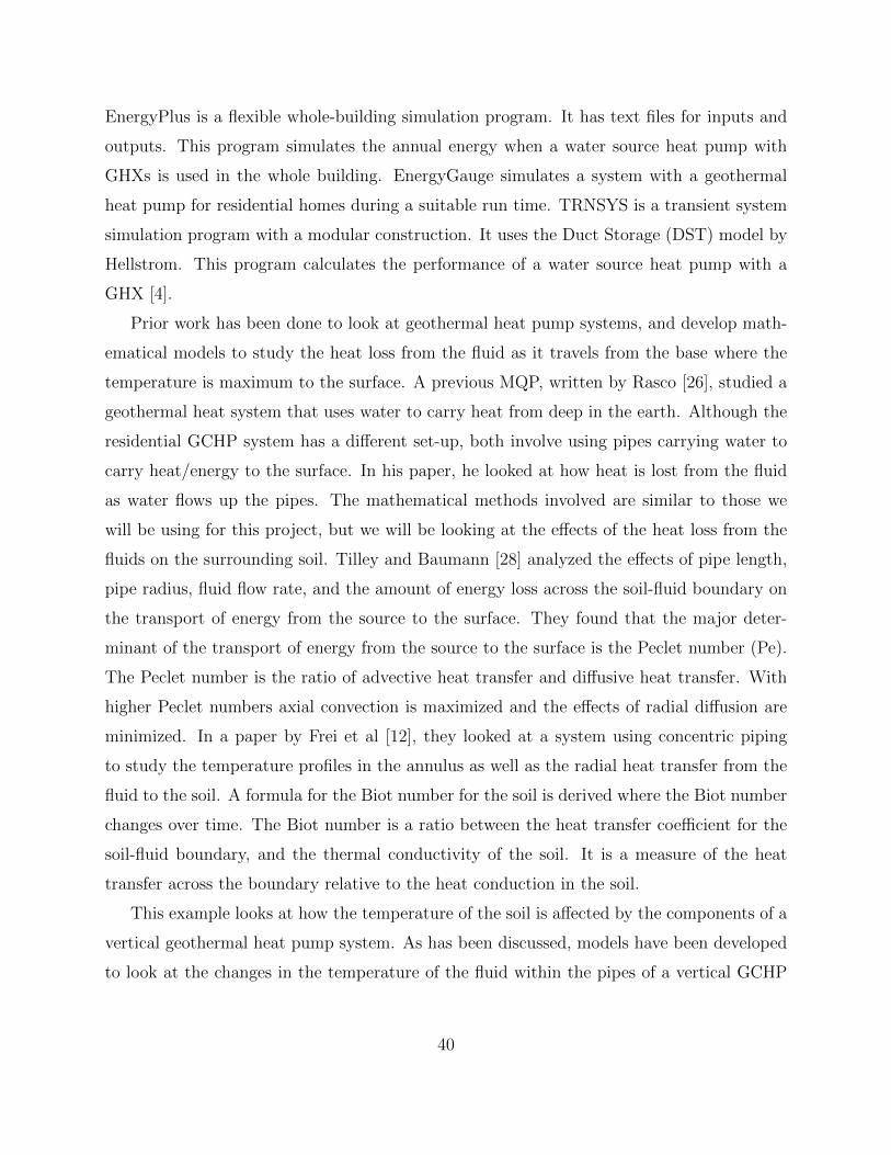
In figure 7.2, you can see how the µ’s (eigenvalues) vary with respect to the β (Biot number).

Each curve is a different µ. As you can see, µ starts high and declines to a value as β

approaches zero. As we increase the index, µ increases.

Figure 7.3 shows how λ varies with respect to β. Each curve is a different λ. As you can

see, λ starts high and declines to a value as β approaches zero. As we increase the index, λ

increases.

Figure 7.4 shows how ψ1, ψ2, ψ3 vary with x for a value of β (β = 5). ψ oscillates as a

function of x. ψ1 does not even have half a period in this domain. ψ2 has a period of about

48

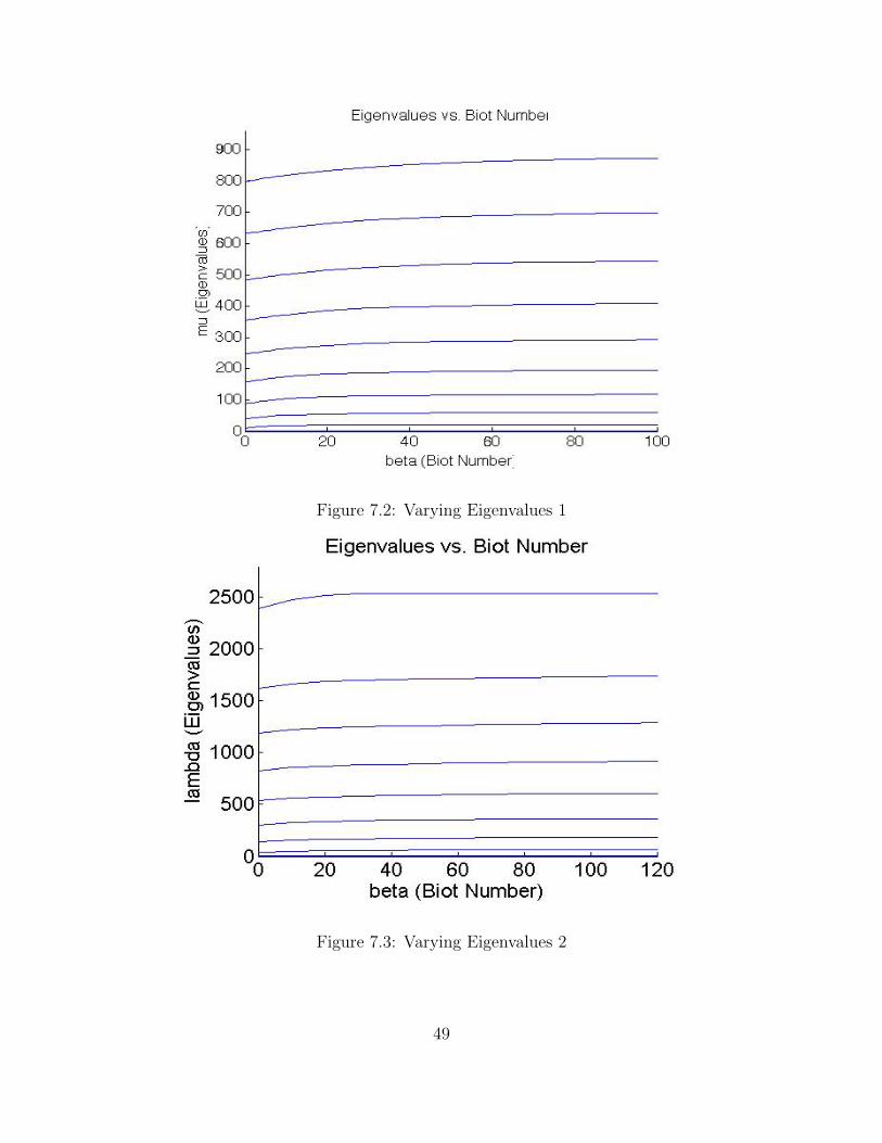
Figure 7.2: Varying Eigenvalues 1

Figure 7.3: Varying Eigenvalues 2

49

Figure 7.4: Varying Eigenfunctions 1


50

.4. ψ3 has a period of about .15. Figure 7.5 shows how ψ1, ψ2, ψ3 vary with x for a different

value of β (β = 20). ψ oscillates as a function of x. ψ1 does not even have half a period in

this domain. ψ2 has a period of about .3. ψ3 has a period of about .1. By comparing these

two graphs, you can see that ψ changes with β.


Figure 7.6 shows how φ1, φ2, φ3 vary with x for a value of β (β = 5). φ oscillates as a

function of x. φ1 does not even have half a period in this domain. φ2 has a period of about

.4. φ3 has a period of about .15. Figure 7.7 shows how φ1, φ2, φ3 vary with x for a different

value of β (β = 20). φ oscillates as a function of x. φ1 does not even have half a period in

this domain. φ2 has a period of about .3. φ3 has a period of about .1. By comparing these

two graphs, you can see that φ changes with β.

Figure 7.8 shows how the temperature changes over β up to a constant multiple. For

simplicity, z = 0, x = 1, and each Aj = 1. If we assume that kskw

= 1, then this graph is for

time from 1π

to ∞.

Given the assumptions, this graph is correct. However, this graph does not fit the physical

model. Notice that the graph has a section that is negative; this should not happen. Also,

51


Figure 7.8: Temperature

52

at the beginning, there should not be a section that increases. The problem is probably the

assumption that each Aj = 1.

If we are given a position (x, z) at time t, then we can find the temperature there. Given

t, we can find β, where

β =kskw

1√πt

in equation (7.8). Now that we know β, we can find our µs by solving equation (7.25)

−√µ sin(√µ) + β cos(

√µ) = 0.

Notice that we get a sequence of µ1, µ2, µ3, .... Now we can use our µs to find the ψs where

ψi = Ci cos(√µix)

from equation (7.26). Next we can find λs and φs by first finding the λ and Cik using equation

(7.28)

M~c = λB~c

then using the C to put together the φs using equation (7.27)

φk =∞∑i=1

Cikψi.

Thus, we can use the λs to find Zs using equation (7.29)

Zi = Aie−λiP e

z.

Since we know the φs and Zs, we can combine the according to equation (7.30) and sum up

to get equation (7.31)

Θ =∑i

φiZi.

Then we can plug in x and z and get a value for the temperature.

53

Chapter 8

Summary

The purpose of this project was to analyze the partial differential equation associated with

the geothermal heat pump. Chapter 6 develops the mathematical model for the heat pump.

In chapter 7, we obtain a formula for the solution to the PDE in terms of eigenfunctions,

which can be approximated numerically. Observe that the soil temperature does change with

respect to time. It appears to increase as time increases. I believe that this could make the

system more efficient as time goes to infinity. More research would have to be done. For one,

this project only looks at half of the system. Another project could look at how this can

be applied to the whole system. Also, someone could look at whether or not this actually

effects the efficiency of the system.

The other purpose of this project was to develop the background needed to solve the

PDE. We assume that the reader is a WPI student who has taken Calculus and Ordinary

Differential Equations. In chapters 2 and 3, we review relevant topics from these courses

that are needed to understand how to solve the PDE. Chapter 4 covers a new type of ODE

call boundary value problems. A BVP can have a solution called an eigenfunction which

corresponds to a specific eigenvalue. In chapter 5, we cover PDEs, specifically the method of

separation of variables, and how this can lead to the need for eigenvalues and eigenfunctions.

54

Appendix A

Matlab

This section includes Matlab codes that were made for this project. The first Matlab file is

a function called froot that finds the roots of −√µ sin(√µ) + β cos(

√µ) = 0. The second

Matlab file is a function called lambda that finds the µs (M), λs (L), and the constants (C).

The third file, called graphs, creates the graphs that were used in chapter 3. The fourth

Matlab file, called geothermal, numerically calculates the µs (M), λs (L), and the constants

(C) as well as creates the graphs seen in section 7.5.

55

1 function mu=froot(m0,B,itmax)

2 f=@(x) B*cos(sqrt(x))-sqrt(x)*sin(sqrt(x));

3 x1=m0(1);

4 x2=m0(2);

5 i=1;

6 while i<itmax

7 x=x2-((x2-x1)/(f(x2)-f(x1)))*f(x2);

8 if abs(f(x))<10ˆ(-10);

9 break

10 end

11 i=i+1;

12 if f(x)*f(x2)<0

13 x1=x2;

14 end

15 x2=x;

16 end

17 mu=[x(i+1)];

56

1 function [L, C, M]=lambda(B)

2 for i=1:10

3 mu1(i)=froot([piˆ2*(i-1)ˆ2,piˆ2*(i-1)ˆ2+.5*i],B,25);

4 end

5

6 syms x

7

8 for i=1:10

9 for j=1:10

10 b1(i,j)=int((1-xˆ2)*cos(sqrt(mu1(i))*x)*cos(sqrt(mu1(j))*x),0,1);

11 end

12 end

13

14 b=double(b1);

15

16

17 M=diag(mu1(:));

18

19

20 [C,L]=eig(M,b);

57

1 %# File name =graphs.m

2 fplot(@(x) sin(x),[-pi/2,pi/2])

3 axis([-pi/2-.5,pi/2+.5,-1.1,1.1])

4

5

6 %# vertical line

7 hx = graph2d.constantline(0, ’LineStyle’,’:’, ’Color’,[.7 .7 .7]);

8 changedependvar(hx,’x’);

9

10 %# horizontal line

11 hy = graph2d.constantline(0, ’Color’,[.7 .7 .7]);

12 changedependvar(hy,’y’);

13

14 %%

15

16 fplot(@(x) 1/(1-x),[-1,1])

17 axis([-1,1.1,-.1,100])

18

19 hx = graph2d.constantline(1, ’LineStyle’,’:’, ’Color’,[.7 .7 .7]);

20 changedependvar(hx,’x’);

21

22

23 %%

24

25 hold on

26

27 fplot(@(x) 0,[0,5])

28 fplot(@(x) .25*xˆ2, [0,5])

29 axis([0,5,-.1,7])

30

58

31 hold off

59

1 %# File name=geothermal.m

2 B=.1;

3 for i=1:10

4 mu1(i,1)=piˆ2*(i-1)ˆ2;

5 mu1(i,2)=froot([piˆ2*(i-1)ˆ2,piˆ2*(i-1)ˆ2+.5*i],B,25);

6 end

7

8 for j=3:11

9 for i=1:10

10 mu1(i,j)=froot([mu1(i,j-1), mu1(i,j-2)],B*(j-1),25);

11 end

12 end

13

14 for i=1:10

15 mu1(i,12)=froot([mu1(i,1),mu1(i,11)],2,25);

16 end

17

18 for j=13:20

19 for i=1:10

20 mu1(i,j)=froot([mu1(i,j-1), mu1(i,j-2)],(j-10),25);

21 end

22 end

23

24 for i=1:10

25 mu1(i,21)=froot([mu1(i,1),mu1(i,20)],20,25);

26 end

27

28 for j=22:29

29 for i=1:10

30 mu1(i,j)=froot([mu1(i,j-1), mu1(i,j-2)],10*(j-19),25);

60

31 end

32 end

33

34 beta=[0,.1,.2,.3,.4,.5,.6,.7,.8,.9,1,2,3,4,5,6,7,8,9,10,20,30,40,50,60,70,80,90,100];

35

36

37 for i=1:10

38 hold on

39 niceplot(beta(:),mu1(i,:),’beta (Biot Number)’,’mu (Eigenvalues)’,’Eigenvalues vs. Biot Number’);

40 end

41

42 %%

43

44 for i=1:12

45 [L(:,:,i+1), C(:,:,i+1), M(:,:,i+1)]=lambda(5*i);

46 end

47

48 [L(:,:,1), C(:,:,1), M(:,:,1)]=lambda(0);

49

50 for i=1:13

51 for j=1:10

52 l(j,i)=L(j,j,i);

53 m(j,i)=M(j,j,i);

54 end

55 end

56

57 for i=1:13

58 p(i)=5*(i-1);

59 end

60

61

61 hold on

62 for i=1:9

63 niceplot(p,l(i,:),’beta (Biot Number)’,’lambda (Eigenvalues)’,’Eigenvalues vs. Biot Number’)

64 end

65 hold off

66

67 %%

68

69 for i=1:10

70 for j=1:100

71 ps1(j,i)=cos(m(i,2)*((1/99)*(j-1)));

72 x(j)=(1/99)*(j-1);

73 end

74 end

75

76 phi1=ps1*C(:,:,2);

77 figure(2)

78 hold on

79 for i=1:3

80 niceplot(x,ps1(:,i),’x’,’psi (Eigenfunctions)’,’Eigenfunctions 1’)

81 end

82 hold off

83 figure(3)

84 hold on

85 for i=1:3

86 niceplot(x,phi1(:,i),’x’,’phi (Eigenfunctions)’,’Eigenfunctions 3’)

87 end

88 hold off

89

90 for i=1:10

62

91 for j=1:100

92 ps2(j,i)=cos(m(i,5)*((1/99)*(j-1)));

93 x(j)=(1/99)*(j-1);

94 end

95 end

96

97 phi2=(ps2*C(:,:,5));

98 figure(4)

99 hold on

100 for i=1:3

101 niceplot(x,ps2(:,i),’x’,’psi (Eigenfunctions)’,’Eigenfunctions 2’)

102 end

103 hold off

104 figure(5)

105 hold on

106 for i=1:3

107 niceplot(x,phi2(:,i),’x’,’phi (Eigenfunctions)’,’Eigenfunctions 4’)

108 end

109 hold off

110

111 %%

112 for i=1:10

113 [L2(:,:,i+1), C2(:,:,i+1), M2(:,:,i+1)]=lambda(.1*i);

114 end

115

116 [L2(:,:,1), C2(:,:,1), M2(:,:,1)]=lambda(0);

117

118 for i=1:11

119 for j=1:10

120 l2(j,i)=L2(j,j,i);

63

121 m2(j,i)=M2(j,j,i);

122 end

123 end

124

125 for i=1:11

126 p2(i)=.1*(i-1);

127 end

128

129 for i=1:10

130 for j=1:11

131 ps3(j,i)=cos(m2(i,j));

132 end

133 end

134 for i=1:11

135 phi3(:,i)=ps3(i,:)*C2(:,:,i);

136 end

137

138

139

140

141 theta=sum(phi3,1);

142 figure(6)

143 niceplot(p2,theta,’beta (Biot number)’,’Temperature’,’Temperature vs Beta’)

64

Bibliography

[1] Al-Khoury, Rafid. Computational Modeling of Shallow Geothermal Systems. First. Lei-

den: CRC Press, 2012. Print.

[2] Carslaw, H.S. and J.C. Jaeger. 1947. Conduction of heat in solids. Oxford, U.K.: Clare-

more Press.

[3] Chiasson, Andrew. Simulation and Design of Hybrid Geothermal Heat Pump Systems.

University of Wyoming. Ann Arbor: ProQuest/UMI, 2007. (Publication No. 3278005).

[4] Cho, Soolyeon, and Sedighehsadat Mirianhosseinabadi. “Simulation Modeling of

Ground Source Heat Pump Systems for the Performance Analysis of Residential Build-

ings.” Proceedings of BS2013: 13th Conference of International Building Performance

Simulation Association. Chambery: 2013. 1960-1967. Print.

[5] “Choosing and Installing Geothermal Heat Pumps.” Energy.gov.

U.S. Department of Energy, 24 Jun 2012. Web. 9 Mar 2014.

<http://energy.gov/energysaver/articles/choosing-and-installing-geothermal-heat-

pumps>.

[6] “COPs, EERs, and SEERs How Efficient is Your Air Conditioning System?.” Power

Knot. Power Knot LLC. Web. 9 Mar 2014. <http://www.powerknot.com/how-efficient-

is-your-air-conditioning-system.html>.

[7] Davis, Paul W. Differential Equations for Mathematics, Science, and Engineering. En-

glewood Cliffs, N.J.: Prentice Hall, 1992. Print.

65

[8] Deerman, J.D. and S.P. Kavanaugh. 1991. Simulation of vertical U-tube ground coupled

heat pump systems using the cylindrical heat source solution. ASHRAE Transactions

97(1): 287?295.

[9] Do, Sung Lok, and Jeff S. Haberl. “A reveiw of ground-coupled heat pump models used

in whole-building computer simulation programs.” Proceedings of the 17th Symposium

for Improving Building Systems in Hot and Humid Climates. Austin: Print.

[10] Farlow, Stanley J. Partial Differential Equations for Scientists and Engineers. New

York: Wiley, 1982. Print.

[11] Farr, William. “Ordinary Differential Equations.” Worcester Polytechnic Institute, . 4

Oct. 2010. Unpublished Lecture Notes.

[12] Frei, S., K. Lockwood, G. Stewart, J. Boyer, and B. Tilley. “On thermal resistance in

concentric residential geothermal heat exchangers.” Springer Science+Business Media

Dordrecht: n. pag. Web.

[13] “Geothermal Heat Pumps.” Energy.gov. U.S. Department of Energy, 24 Jun 2012. Web.

9 Mar 2014. <http://energy.gov/energysaver/articles/geothermal-heat-pumps >.

[14] “Geothermal Pipe: What to Use and What to Stay Away From.” Geother-

mal Pros and Cons. Geothermal Pros and Cons, 10 May 2012. Web. 9 Mar.

2014. <http://geothermalprosandcons.net/geothermal-pipe-what-to-use-and-what-to-

stay-away-from/>.

[15] “GSHP - Ground Source Heat Pump.” ICAX. ICAX, n.d. Web. 9 Mar 2014.

<http://www.icax.co.uk/ gshp.html>.

[16] Hackel, Scott, Gregory Nellis, and Sanford Klein. “Optimization of Hybrid Geothermal

Heat Pump Systems.” 9th International IEA Heat Pump Conference. Zurich: Print.

[17] “Heat Pumps.” ICAX. ICAX, n.d. Web. 9 Mar 2014.

<http://www.icax.co.uk/Heat Pumps.html>.

66

[18] “The History of Geothermal Energy.” Geothermal Utilities. N.p.. Web. 9 Mar 2014.

<http://www. geoutilities.ca/about geothermal/history.html>.

[19] Howard, Brian Clark. N.p., n. d. 9 Mar 2014.

<http://energyblog.nationalgeographic.com/2013/09/17/10-myths-about-geothermal-

heating-and-cooling/>.

[20] Larson, Ron, Robert P. Hostetler, and Bruce Edwards. Calculus with analytic geometry.

8th ed. Boston: Houghton Mifflin Co., 2006. Print.

[21] Lawson, Terry. “How Much Room Outside Do I Need for a Geothermal System?.” New

River Heating & Air. New River Heating & Air, Inc., 15 Mar 2011. Web. 11 Mar 2014.

[22] “Loop Configurations for Geothermal Systems.” Kocher’s Water Pumps and Tanks.

N.p., n.d. Web. 9 Mar 2014.

[23] Maehlum, Mathias. “Geothermal Heating and Cooling Systems.” . Energy Informative,

2 May 2013. Web. 7 May 2014. <http://energyinformative.org/geothermal-heating-and-

cooling-systems/>.

[24] “Mean Annual Air Temperature.” ICAX. ICAX, n.d. Web. 9 Mar 2014.

<http://www.icax.co.uk/Mean Annual Air Temperature.html>.

[25] Rafferty, Kevin. “Piping Geothermal Fluids.” Trans. Array Geothermal Direct Use En-

gineering and Design Guidebook. Third Edition. Klamath Falls, OR: Geo-Heat Center,

Oregon Institute of Technology, 1998. Chapter 10. Print.

[26] Rasco, Miguel.A. “Boundary Value Problems in Geothermal Heat.” MQP Report ad-

vised by B.S. Tilley August 2011

[27] “Seasonal Performance Factor.” ICAX. ICAX, n.d. Web. 9 Mar 2014.

<http://www.icax.co.uk/Seasonal Performance Factor.html>.

[28] Tilley,B. and T. Baumann. “On temperature attenuation in staged open-loop wells”

Renewable Energy 48 (2012) 416-423.

67

[29] United States. Environmental Protection Agency. Environmental Technology Verifica-

tion Report:ECR Technologies, Inc. EarthLinked Ground-Source Heat Pump Water

Heating System. Research Triangle Park: U.S. Environmental Protection Agency, 2006.

Print.

[30] Yang, H., P. Cui, and Z. Fang. “Vertical-borehole ground-coupled heat pumps: A review

of models and systems.” Applied Energy. 87.1 (2010): 16 - 27. Print.

[31] Yavuzturk, C., J.D. Spitler. 1999. A Short Time Step Response Factor Model for Vertical

Ground Loop Heat Exchangers. ASHRAE Transactions. 105(2): 475-485.

68

a tutorial approach to the analysis of a geothermal ... · project number: mb8-aamx a tutorial...

Documents