A Tutorial Introduction to the

Minimum Description Length Principle

Peter Grunwald

Centrum voor Wiskunde en Informatica

Kruislaan 413, 1098 SJ Amsterdam

The Netherlands

pdg@cwi.nl

www.grunwald.nl

Abstract

This tutorial provides an overview of and introduction to Rissanen’s Minimum De-scription Length (MDL) Principle. The first chapter provides a conceptual, entirelynon-technical introduction to the subject. It serves as a basis for the technical intro-duction given in the second chapter, in which all the ideas of the first chapter are mademathematically precise. This tutorial will appear as the first two chapters in the collec-tion Advances in Minimum Description Length: Theory and Applications [Grunwald,Myung, and Pitt 2004], to be published by the MIT Press.

Contents

1 Introducing MDL 51.1 Introduction and Overview . . . . . . . . . . . . . . . . . . . . . . . . . 51.2 The Fundamental Idea:

Learning as Data Compression . . . . . . . . . . . . . . . . . . . . . . . 61.2.1 Kolmogorov Complexity and Ideal MDL . . . . . . . . . . . . . . 81.2.2 Practical MDL . . . . . . . . . . . . . . . . . . . . . . . . . . . . 8

1.3 MDL and Model Selection . . . . . . . . . . . . . . . . . . . . . . . . . . 91.4 Crude and Refined MDL . . . . . . . . . . . . . . . . . . . . . . . . . . . 121.5 The MDL Philosophy . . . . . . . . . . . . . . . . . . . . . . . . . . . . 141.6 MDL and Occam’s Razor . . . . . . . . . . . . . . . . . . . . . . . . . . 171.7 History . . . . . . . . . . . . . . . . . . . . . . . . . . . . . . . . . . . . 191.8 Summary and Outlook . . . . . . . . . . . . . . . . . . . . . . . . . . . . 20

2 Tutorial on MDL 232.1 Plan of the Tutorial . . . . . . . . . . . . . . . . . . . . . . . . . . . . . 232.2 Information Theory I: Probabilities and Codelengths . . . . . . . . . . . 24

2.2.1 Prefix Codes . . . . . . . . . . . . . . . . . . . . . . . . . . . . . 252.2.2 The Kraft Inequality - Codelengths & Probabilities, I . . . . . . 262.2.3 The Information Inequality - Codelengths & Probabilities, II . . 31

2.3 Statistical Preliminaries and Example Models . . . . . . . . . . . . . . . 322.4 Crude MDL . . . . . . . . . . . . . . . . . . . . . . . . . . . . . . . . . . 34

2.4.1 Description Length of Data given Hypothesis . . . . . . . . . . . 352.4.2 Description Length of Hypothesis . . . . . . . . . . . . . . . . . . 35

2.5 Information Theory II: Universal Codes and Models . . . . . . . . . . . 372.5.1 Two-part Codes as simple Universal Codes . . . . . . . . . . . . 392.5.2 From Universal Codes to Universal Models . . . . . . . . . . . . 402.5.3 NML as an Optimal Universal Model . . . . . . . . . . . . . . . . 42

2.6 Simple Refined MDL and its Four Interpretations . . . . . . . . . . . . . 442.6.1 Compression Interpretation . . . . . . . . . . . . . . . . . . . . . 462.6.2 Counting Interpretation . . . . . . . . . . . . . . . . . . . . . . . 462.6.3 Bayesian Interpretation . . . . . . . . . . . . . . . . . . . . . . . 492.6.4 Prequential Interpretation . . . . . . . . . . . . . . . . . . . . . . 51

3

2.7 General Refined MDL: Gluing it All Together . . . . . . . . . . . . . . . 542.7.1 Model Selection with Infinitely Many Models . . . . . . . . . . . 542.7.2 The Infinity Problem . . . . . . . . . . . . . . . . . . . . . . . . . 552.7.3 The General Picture . . . . . . . . . . . . . . . . . . . . . . . . . 58

2.8 Beyond Parametric Model Selection . . . . . . . . . . . . . . . . . . . . 602.9 Relations to Other Approaches to Inductive Inference . . . . . . . . . . 63

2.9.1 What is ‘MDL’? . . . . . . . . . . . . . . . . . . . . . . . . . . . 642.9.2 MDL and Bayesian Inference . . . . . . . . . . . . . . . . . . . . 642.9.3 MDL, Prequential Analysis and Cross-Validation . . . . . . . . . 672.9.4 Kolmogorov Complexity and Structure Function; Ideal MDL . . 67

2.10 Problems for MDL? . . . . . . . . . . . . . . . . . . . . . . . . . . . . . 682.10.1 Conceptual Problems: Occam’s Razor . . . . . . . . . . . . . . . 692.10.2 Practical Problems with MDL . . . . . . . . . . . . . . . . . . . 70

2.11 Conclusion . . . . . . . . . . . . . . . . . . . . . . . . . . . . . . . . . . 71

4

Chapter 1

Introducing the MDL Principle

1.1 Introduction and Overview

How does one decide among competing explanations of data given limited observations?This is the problem of model selection. It stands out as one of the most importantproblems of inductive and statistical inference. The Minimum Description Length(MDL) Principle is a relatively recent method for inductive inference that provides ageneric solution to the model selection problem. MDL is based on the following insight:any regularity in the data can be used to compress the data, i.e. to describe it usingfewer symbols than the number of symbols needed to describe the data literally. Themore regularities there are, the more the data can be compressed. Equating ‘learning’with ‘finding regularity’, we can therefore say that the more we are able to compressthe data, the more we have learned about the data. Formalizing this idea leads to ageneral theory of inductive inference with several attractive properties:

1. Occam’s Razor MDL chooses a model that trades-off goodness-of-fit on the ob-served data with ‘complexity’ or ‘richness’ of the model. As such, MDL embodiesa form of Occam’s Razor, a principle that is both intuitively appealing and infor-mally applied throughout all the sciences.

2. No overfitting, automatically MDL procedures automatically and inherently pro-tect against overfitting and can be used to estimate both the parameters and thestructure (e.g., number of parameters) of a model. In contrast, to avoid over-fitting when estimating the structure of a model, traditional methods such asmaximum likelihood must be modified and extended with additional, typically adhoc principles.

3. Bayesian interpretation MDL is closely related to Bayesian inference, but avoidssome of the interpretation difficulties of the Bayesian approach1, especially in therealistic case when it is known a priori to the modeler that none of the modelsunder consideration is true. In fact:

5

4. No need for ‘underlying truth’ In contrast to other statistical methods, MDLprocedures have a clear interpretation independent of whether or not there existssome underlying ‘true’ model.

5. Predictive interpretation Because data compression is formally equivalent to aform of probabilistic prediction, MDL methods can be interpreted as searchingfor a model with good predictive performance on unseen data.

In this chapter, we introduce the MDL Principle in an entirely non-technical way,concentrating on its most important applications, model selection and avoiding over-fitting. In Section 1.2 we discuss the relation between learning and data compression.Section 1.3 introduces model selection and outlines a first, ‘crude’ version of MDL thatcan be applied to model selection. Section 1.4 indicates how these ‘crude’ ideas needto be refined to tackle small sample sizes and differences in model complexity betweenmodels with the same number of parameters. Section 1.5 discusses the philosophy un-derlying MDL, and considers its relation to Occam’s Razor. Section 1.7 briefly discussesthe history of MDL. All this is summarized in Section 1.8.

1.2 The Fundamental Idea:

Learning as Data Compression

We are interested in developing a method for learning the laws and regularities in data.The following example will illustrate what we mean by this and give a first idea of howit can be related to descriptions of data.

Regularity . . . Consider the following three sequences. We assume that each se-quence is 10000 bits long, and we just list the beginning and the end of each sequence.

00010001000100010001 . . . 0001000100010001000100010001 (1.1)

01110100110100100110 . . . 1010111010111011000101100010 (1.2)

00011000001010100000 . . . 0010001000010000001000110000 (1.3)

The first of these three sequences is a 2500-fold repetition of 0001. Intuitively, thesequence looks regular; there seems to be a simple ‘law’ underlying it; it might makesense to conjecture that future data will also be subject to this law, and to predictthat future data will behave according to this law. The second sequence has beengenerated by tosses of a fair coin. It is intuitively speaking as ‘random as possible’, andin this sense there is no regularity underlying it. Indeed, we cannot seem to find such aregularity either when we look at the data. The third sequence contains approximatelyfour times as many 0s as 1s. It looks less regular, more random than the first; but itlooks less random than the second. There is still some discernible regularity in thesedata, but of a statistical rather than of a deterministic kind. Again, noticing that sucha regularity is there and predicting that future data will behave according to the sameregularity seems sensible.

6

...and Compression We claimed that any regularity detected in the data can be usedto compress the data, i.e. to describe it in a short manner. Descriptions are alwaysrelative to some description method which maps descriptions D′ in a unique manner todata sets D. A particularly versatile description method is a general-purpose computerlanguage like C or Pascal. A description of D is then any computer program thatprints D and then halts. Let us see whether our claim works for the three sequencesabove. Using a language similar to Pascal, we can write a program

for i = 1 to 2500; print ‘0001‘; next; halt

which prints sequence (1) but is clearly a lot shorter. Thus, sequence (1) is indeedhighly compressible. On the other hand, we show in Section 2.2, that if one generatesa sequence like (2) by tosses of a fair coin, then with extremely high probability, theshortest program that prints (2) and then halts will look something like this:

print ‘011101001101000010101010........1010111010111011000101100010‘; halt

This program’s size is about equal to the length of the sequence. Clearly, it does nothingmore than repeat the sequence.

The third sequence lies in between the first two: generalizing n = 10000 to arbitrarylength n, we show in Section 2.2 that the first sequence can be compressed to O(logn)bits; with overwhelming probability, the second sequence cannot be compressed at all;and the third sequence can be compressed to some length αn, with 0 < α < 1.

Example 1.1 [compressing various regular sequences] The regularities underly-ing sequences (1) and (3) were of a very particular kind. To illustrate that any typeof regularity in a sequence may be exploited to compress that sequence, we give a fewmore examples:

The Number π Evidently, there exists a computer program for generating the firstn digits of π – such a program could be based, for example, on an infinite se-ries expansion of π. This computer program has constant size, except for thespecification of n which takes no more than O(logn) bits. Thus, when n is verylarge, the size of the program generating the first n digits of π will be very smallcompared to n: the π-digit sequence is deterministic, and therefore extremelyregular.

Physics Data Consider a two-column table where the first column contains numbersrepresenting various heights from which an object was dropped. The second col-umn contains the corresponding times it took for the object to reach the ground.Assume both heights and times are recorded to some finite precision. In Sec-tion 1.3 we illustrate that such a table can be substantially compressed by firstdescribing the coefficients of the second-degree polynomial H that expresses New-ton’s law; then describing the heights; and then describing the deviation of thetime points from the numbers predicted by H.

7

Natural Language Most sequences of words are not valid sentences according to theEnglish language. This fact can be exploited to substantially compress Englishtext, as long as it is syntactically mostly correct: by first describing a grammarfor English, and then describing an English text D with the help of that grammar[Grunwald 1996], D can be described using much less bits than are needed withoutthe assumption that word order is constrained.

1.2.1 Kolmogorov Complexity and Ideal MDL

To formalize our ideas, we need to decide on a description method, that is, a formallanguage in which to express properties of the data. The most general choice is ageneral-purpose2 computer language such as C or Pascal. This choice leads to thedefinition of the Kolmogorov Complexity [Li and Vitanyi 1997] of a sequence as thelength of the shortest program that prints the sequence and then halts. The lower theKolmogorov complexity of a sequence, the more regular it is. This notion seems to behighly dependent on the particular computer language used. However, it turns out thatfor every two general-purpose programming languages A and B and every data sequenceD, the length of the shortest program for D written in language A and the length of theshortest program forD written in language B differ by no more than a constant c, whichdoes not depend on the length of D. This so-called invariance theorem says that, aslong as the sequence D is long enough, it is not essential which computer language onechooses, as long as it is general-purpose. Kolmogorov complexity was introduced, andthe invariance theorem was proved, independently by Kolmogorov [1965], Chaitin [1969]and Solomonoff [1964]. Solomonoff’s paper, called A Theory of Inductive Inference,contained the idea that the ultimate model for a sequence of data may be identifiedwith the shortest program that prints the data. Solomonoff’s ideas were later extendedby several authors, leading to an ‘idealized’ version of MDL [Solomonoff 1978; Li andVitanyi 1997; Gacs, Tromp, and Vitanyi 2001]. This idealized MDL is very general inscope, but not practically applicable, for the following two reasons:

1. uncomputability It can be shown that there exists no computer program that,for every set of data D, when given D as input, returns the shortest program thatprints D [Li and Vitanyi 1997].

2. arbitrariness/dependence on syntax In practice we are confronted with smalldata samples for which the invariance theorem does not say much. Then thehypothesis chosen by idealized MDL may depend on arbitrary details of the syntaxof the programming language under consideration.

1.2.2 Practical MDL

Like most authors in the field, we concentrate here on non-idealized, practical versionsof MDL that explicitly deal with the two problems mentioned above. The basic ideais to scale down Solomonoff’s approach so that it does become applicable. This is

8

achieved by using description methods that are less expressive than general-purposecomputer languages. Such description methods C should be restrictive enough so thatfor any data sequence D, we can always compute the length of the shortest descriptionof D that is attainable using method C; but they should be general enough to allow usto compress many of the intuitively ‘regular’ sequences. The price we pay is that, usingthe ‘practical’ MDL Principle, there will always be some regular sequences which wewill not be able to compress. But we already know that there can be no method forinductive inference at all which will always give us all the regularity there is — simplybecause there can be no automated method which for any sequence D finds the shortestcomputer program that prints D and then halts. Moreover, it will often be possible toguide a suitable choice of C by a priori knowledge we have about our problem domain.For example, below we consider a description method C that is based on the class ofall polynomials, such that with the help of C we can compress all data sets which canmeaningfully be seen as points on some polynomial.

1.3 MDL and Model Selection

Let us recapitulate our main insights so far:

MDL: The Basic IdeaThe goal of statistical inference may be cast as trying to find regularity in the data.‘Regularity’ may be identified with ‘ability to compress’. MDL combines these twoinsights by viewing learning as data compression: it tells us that, for a given set ofhypotheses H and data set D, we should try to find the hypothesis or combinationof hypotheses in H that compresses D most.

This idea can be applied to all sorts of inductive inference problems, but it turns out tobe most fruitful in (and its development has mostly concentrated on) problems of modelselection and, more generally, dealing with overfitting. Here is a standard example (weexplain the difference between ‘model’ and ‘hypothesis’ after the example).

Example 1.2 [Model Selection and Overfitting] Consider the points in Figure 1.1.We would like to learn how the y-values depend on the x-values. To this end, we maywant to fit a polynomial to the points. Straightforward linear regression will giveus the leftmost polynomial - a straight line that seems overly simple: it does notcapture the regularities in the data well. Since for any set of n points there exists apolynomial of the (n − 1)-st degree that goes exactly through all these points, simplylooking for the polynomial with the least error will give us a polynomial like the onein the second picture. This polynomial seems overly complex: it reflects the randomfluctuations in the data rather than the general pattern underlying it. Instead of pickingthe overly simple or the overly complex polynomial, it seems more reasonable to prefera relatively simple polynomial with small but nonzero error, as in the rightmost picture.

9

Figure 1.1: A simple, a complex and a trade-off (3rd degree) polynomial.

This intuition is confirmed by numerous experiments on real-world data from a broadvariety of sources [Rissanen 1989; Vapnik 1998; Ripley 1996]: if one naively fits a high-degree polynomial to a small sample (set of data points), then one obtains a very goodfit to the data. Yet if one tests the inferred polynomial on a second set of data comingfrom the same source, it typically fits this test data very badly in the sense that thereis a large distance between the polynomial and the new data points. We say that thepolynomial overfits the data. Indeed, all model selection methods that are used inpractice either implicitly or explicitly choose a trade-off between goodness-of-fit andcomplexity of the models involved. In practice, such trade-offs lead to much betterpredictions of test data than one would get by adopting the ‘simplest’ (one degree)or most ‘complex3’ (n− 1-degree) polynomial. MDL provides one particular means ofachieving such a trade-off.

It will be useful to make a precise distinction between ‘model’ and ‘hypothesis’:

Models vs. HypothesesWe use the phrase point hypothesis to refer to a single probability distribution orfunction. An example is the polynomial 5x2 + 4x + 3. A point hypothesis is alsoknown as a ‘simple hypothesis’ in the statistical literature.We use the word model to refer to a family (set) of probability distributions orfunctions with the same functional form. An example is the set of all second-degree polynomials. A model is also known as a ‘composite hypothesis’ in thestatistical literature.We use hypothesis as a generic term, referring to both point hypotheses and mod-els.

In our terminology, the problem described in Example 1.2 is a ‘hypothesis selectionproblem’ if we are interested in selecting both the degree of a polynomial and the cor-responding parameters; it is a ‘model selection problem’ if we are mainly interested in

10

selecting the degree.

To apply MDL to polynomial or other types of hypothesis and model selection, wehave to make precise the somewhat vague insight ‘learning may be viewed as datacompression’. This can be done in various ways. In this section, we concentrate on theearliest and simplest implementation of the idea. This is the so-called two-part codeversion of MDL:

Crude4, Two-part Version of MDL Principle (Informally Stated)Let H(1),H(2), . . . be a list of candidate models (e.g., H(k) is the set of k-th degreepolynomials), each containing a set of point hypotheses (e.g., individual polynomi-als). The best point hypothesis H ∈ H(1) ∪H(2) ∪ . . . to explain the data D is theone which minimizes the sum L(H) + L(D|H), where

• L(H) is the length, in bits, of the description of the hypothesis; and

• L(D|H) is the length, in bits, of the description of the data when encodedwith the help of the hypothesis.

The best model to explain D is the smallest model containing the selected H.

Example 1.3 [Polynomials, cont.] In our previous example, the candidate hypothe-ses were polynomials. We can describe a polynomial by describing its coefficients in acertain precision (number of bits per parameter). Thus, the higher the degree of a poly-nomial or the precision, the more5 bits we need to describe it and the more ‘complex’it becomes. A description of the data ‘with the help of’ a hypothesis means that thebetter the hypothesis fits the data, the shorter the description will be. A hypothesisthat fits the data well gives us a lot of information about the data. Such informationcan always be used to compress the data (Section 2.2). Intuitively, this is because weonly have to code the errors the hypothesis makes on the data rather than the full data.In our polynomial example, the better a polynomial H fits D, the fewer bits we needto encode the discrepancies between the actual y-values yi and the predicted y-valuesH(xi). We can typically find a very complex point hypothesis (large L(H)) with a verygood fit (small L(D|H)). We can also typically find a very simple point hypothesis(small L(H)) with a rather bad fit (large L(D|H)). The sum of the two descriptionlengths will be minimized at a hypothesis that is quite (but not too) ‘simple’, with agood (but not perfect) fit.

11

1.4 Crude and Refined MDL

Crude MDL picks the H minimizing the sum L(H)+L(D|H). To make this procedurewell-defined, we need to agree on precise definitions for the codes (description methods)giving rise to lengths L(D|H) and L(H). We now discuss these codes in more detail.We will see that the definition of L(H) is problematic, indicating that we somehowneed to ‘refine’ our crude MDL Principle.

Definition of L(D|H) Consider a two-part code as described above, and assume forthe time being that all H under consideration define probability distributions. If H isa polynomial, we can turn it into a distribution by making the additional assumptionthat the Y -values are given by Y = H(X)+Z, where Z is a normally distributed noiseterm.

For each H we need to define a code with length L(· | H) such that L(D|H)can be interpreted as ‘the codelength of D when encoded with the help of H’. Itturns out that for probabilistic hypotheses, there is only one reasonable choice forthis code. It is the so-called Shannon-Fano code, satisfying, for all data sequencesD, L(D|H) = − logP (D|H), where P (D|H) is the probability mass or density of Daccording to H – such a code always exists, Section 2.2.

Definition of L(H): A Problem for Crude MDL It is more problematic to finda good code for hypotheses H. Some authors have simply used ‘intuitively reasonable’codes in the past, but this is not satisfactory: since the description length L(H) ofany fixed point hypothesis H can be very large under one code, but quite short underanother, our procedure is in danger of becoming arbitrary. Instead, we need some addi-tional principle for designing a code for H. In the first publications on MDL [Rissanen1978; Rissanen 1983], it was advocated to choose some sort of minimax code for H,minimizing, in some precisely defined sense, the shortest worst-case total descriptionlength L(H)+L(D|H), where the worst-case is over all possible data sequences. Thus,the MDL Principle is employed at a ‘meta-level’ to choose a code for H. However, thiscode requires a cumbersome discretization of the model space H, which is not alwaysfeasible in practice. Alternatively, Barron [1985] encoded H by the shortest computerprogram that, when input D, computes P (D|H). While it can be shown that thisleads to similar codelengths, it is computationally problematic. Later, Rissanen [1984]realized that these problems could be side-stepped by using a one-part rather than atwo-part code. This development culminated in 1996 in a completely precise prescrip-tion of MDL for many, but certainly not all practical situations [Rissanen 1996]. Wecall this modern version of MDL refined MDL:

Refined MDL In refined MDL, we associate a code for encoding D not with a singleH ∈ H, but with the full model H. Thus, given model H, we encode data not in twoparts but we design a single one-part code with lengths L(D|H). This code is designedsuch that whenever there is a member of (parameter in) H that fits the data well, in

12

the sense that L(D | H) is small, then the codelength L(D|H) will also be small. Codeswith this property are called universal codes in the information-theoretic literature[Barron, Rissanen, and Yu 1998]. Among all such universal codes, we pick the one thatis minimax optimal in a sense made precise in Section 2.5. For example, the set H(3) ofthird-degree polynomials is associated with a code with lengths L(· | H(3)) such that,the better the data D are fit by the best-fitting third-degree polynomial, the shorterthe codelength L(D | H). L(D | H) is called the stochastic complexity of the data giventhe model.

Parametric Complexity The second fundamental concept of refined MDL is theparametric complexity of a parametric model H which we denote by COMP(H). Thisis a measure of the ‘richness’ of model H, indicating its ability to fit random data.This complexity is related to the degrees-of-freedom in H, but also to the geometricalstructure of H; see Example 1.4. To see how it relates to stochastic complexity, let, forgiven data D, H denote the distribution in H which maximizes the probability, andhence minimizes the codelength L(D | H) of D. It turns out that

stochastic complexity of D given H = L(D | H) +COMP(H).

Refined MDL model selection between two parametric models (such as the models offirst and second degree polynomials) now proceeds by selecting the model such thatthe stochastic complexity of the given data D is smallest. Although we used a one-partcode to encode data, refined MDL model selection still involves a trade-off between twoterms: a goodness-of-fit term L(D | H) and a complexity term COMP(H). However,because we do not explicitly encode hypotheses H any more, there is no arbitrarinessany more. The resulting procedure can be interpreted in several different ways, someof which provide us with rationales for MDL beyond the pure coding interpretation(Sections 2.6.1–2.6.4):

1. Counting/differential geometric interpretation The parametric complexity ofa model is the logarithm of the number of essentially different, distinguishablepoint hypotheses within the model.

2. Two-part code interpretation For large samples, the stochastic complexity canbe interpreted as a two-part codelength of the data after all, where hypotheses Hare encoded with a special code that works by first discretizing the model spaceH into a set of ‘maximally distinguishable hypotheses’, and then assigning equalcodelength to each of these.

3. Bayesian interpretation In many cases, refined MDL model selection coincideswith Bayes factor model selection based on a non-informative prior such as Jef-freys’ prior [Bernardo and Smith 1994].

4. Prequential interpretation Refined MDL model selection can be interpreted asselecting the model with the best predictive performance when sequentially pre-dicting unseen test data, in the sense described in Section 2.6.4. This makes it

13

an instance of Dawid’s [1984] prequential model validation and also relates it tocross-validation methods.

Refined MDL allows us to compare models of different functional form. It even accountsfor the phenomenon that different models with the same number of parameters maynot be equally ‘complex’:

Example 1.4 Consider two models from psychophysics describing the relationship be-tween physical dimensions (e.g., light intensity) and their psychological counterparts(e.g. brightness) [Myung, Balasubramanian, and Pitt 2000]: y = axb + Z (Stevens’model) and y = a ln(x + b) + Z (Fechner’s model) where Z is a normally distributednoise term. Both models have two free parameters; nevertheless, it turns out that ina sense, Stevens’ model is more flexible or complex than Fechner’s. Roughly speaking,this means there are a lot more data patterns that can be explained by Stevens’ modelthan can be explained by Fechner’s model. Myung, Balasubramanian, and Pitt [2000]generated many samples of size 4 from Fechner’s model, using some fixed parametervalues. They then fitted both models to each sample. In 67% of the trials, Stevens’model fitted the data better than Fechner’s, even though the latter generated the data.Indeed, in refined MDL, the ‘complexity’ associated with Stevens’ model is much largerthan the complexity associated with Fechner’s, and if both models fit the data equallywell, MDL will prefer Fechner’s model.

Summarizing, refined MDL removes the arbitrary aspect of crude, two-part code MDLand associates parametric models with an inherent ‘complexity’ that does not dependon any particular description method for hypotheses. We should, however, warn thereader that we only discussed a special, simple situation in which we compared a finitenumber of parametric models that satisfy certain regularity conditions. Whenever themodels do not satisfy these conditions, or if we compare an infinite number of models,then the refined ideas have to be extended. We then obtain a ‘general’ refined MDLPrinciple, which employs a combination of one-part and two-part codes.

1.5 The MDL Philosophy

The first central MDL idea is that every regularity in data may be used to compressthat data; the second central idea is that learning can be equated with finding regu-larities in data. Whereas the first part is relatively straightforward, the second part ofthe idea implies that methods for learning from data must have a clear interpretationindependent of whether any of the models under consideration is ‘true’ or not. QuotingJ. Rissanen [1989], the main originator of MDL:

“We never want to make the false assumption that the observed data actuallywere generated by a distribution of some kind, say Gaussian, and then go onto analyze the consequences and make further deductions. Our deductions may

14

be entertaining but quite irrelevant to the task at hand, namely, to learn usefulproperties from the data.”

Jorma Rissanen [1989]

Based on such ideas, Rissanen has developed a radical philosophy of learning andstatistical inference that is considerably different from the ideas underlying mainstreamstatistics, both frequentist and Bayesian. We now describe this philosophy in moredetail:

1. Regularity as Compression According to Rissanen, the goal of inductive in-ference should be to ‘squeeze out as much regularity as possible’ from the given data.The main task for statistical inference is to distill the meaningful information presentin the data, i.e. to separate structure (interpreted as the regularity, the ‘meaningfulinformation’) from noise (interpreted as the ‘accidental information’). For the threesequences of Example 1.2, this would amount to the following: the first sequence wouldbe considered as entirely regular and ‘noiseless’. The second sequence would be con-sidered as entirely random - all information in the sequence is accidental, there is nostructure present. In the third sequence, the structural part would (roughly) be thepattern that 4 times as many 0s than 1s occur; given this regularity, the descriptionof exactly which of all sequences with four times as many 0s than 1s occurs, is theaccidental information.

2. Models as Languages Rissanen interprets models (sets of hypotheses) as nothingmore than languages for describing useful properties of the data – a modelH is identifiedwith its corresponding universal code L(· | H). Different individual hypotheses withinthe models express different regularities in the data, and may simply be regarded asstatistics, that is, summaries of certain regularities in the data. These regularities arepresent and meaningful independently of whether some H∗ ∈ H is the ‘true state ofnature’ or not. Suppose that the model H under consideration is probabilistic. Intraditional theories, one typically assumes that some P ∗ ∈ H generates the data, andthen ‘noise’ is defined as a random quantity relative to this P ∗. In the MDL view‘noise’ is defined relative to the model H as the residual number of bits needed toencode the data once the model H is given. Thus, noise is not a random variable: itis a function only of the chosen model and the actually observed data. Indeed, thereis no place for a ‘true distribution’ or a ‘true state of nature’ in this view – there areonly models and data. To bring out the difference to the ordinary statistical viewpoint,consider the phrase ‘these experimental data are quite noisy’. According to a traditionalinterpretation, such a statement means that the data were generated by a distributionwith high variance. According to the MDL philosophy, such a phrase means only thatthe data are not compressible with the currently hypothesized model – as a matter ofprinciple, it can never be ruled out that there exists a different model under which thedata are very compressible (not noisy) after all!

15

3. We Have Only the Data Many (but not all6) other methods of inductiveinference are based on the idea that there exists some ‘true state of nature’, typicallya distribution assumed to lie in some model H. The methods are then designed as ameans to identify or approximate this state of nature based on as little data as possible.According to Rissanen7, such methods are fundamentally flawed. The main reason isthat the methods are designed under the assumption that the true state of nature isin the assumed model H, which is often not the case. Therefore, such methods onlyadmit a clear interpretation under assumptions that are typically violated in practice.Many cherished statistical methods are designed in this way - we mention hypothesistesting, minimum-variance unbiased estimation, several non-parametric methods, andeven some forms of Bayesian inference – see Example 2.22. In contrast, MDL has aclear interpretation which depends only on the data, and not on the assumption of anyunderlying ‘state of nature’.

Example 1.5 [Models that are Wrong, yet Useful] Even though the modelsunder consideration are often wrong, they can nevertheless be very useful. Ex-amples are the successful ‘Naive Bayes’ model for spam filtering, Hidden MarkovModels for speech recognition (is speech a stationary ergodic process? probablynot), and the use of linear models in econometrics and psychology. Since thesemodels are evidently wrong, it seems strange to base inferences on them usingmethods that are designed under the assumption that they contain the true distri-bution. To be fair, we should add that domains such as spam filtering and speechrecognition are not what the fathers of modern statistics had in mind when theydesigned their procedures – they were usually thinking about much simpler do-mains, where the assumption that some distribution P ∗ ∈ H is ‘true’ may not beso unreasonable.

4. MDL and Consistency Let H be a probabilistic model, such that each P ∈ H isa probability distribution. Roughly, a statistical procedure is called consistent relativeto H if, for all P ∗ ∈ H, the following holds: suppose data are distributed accordingto P ∗. Then given enough data, the learning method will learn a good approximationof P ∗ with high probability. Many traditional statistical methods have been designedwith consistency in mind (Section 2.3).

The fact that in MDL, we do not assume a true distribution may suggest that we donot care about statistical consistency. But this is not the case: we would still like ourstatistical method to be such that in the idealized case where one of the distributions inone of the models under consideration actually generates the data, our method is ableto identify this distribution, given enough data. If even in the idealized special casewhere a ‘truth’ exists within our models, the method fails to learn it, then we certainlycannot trust it to do something reasonable in the more general case, where there maynot be a ‘true distribution’ underlying the data at all. So: consistency is importantin the MDL philosophy, but it is used as a sanity check (for a method that has beendeveloped without making distributional assumptions) rather than as a design principle.

In fact, mere consistency is not sufficient. We would like our method to convergeto the imagined true P ∗ fast, based on as small a sample as possible. Two-part code

16

MDL with ‘clever’ codes achieves good rates of convergence in this sense (Barron andCover [1991], complemented by [Zhang 2004], show that in many situations, the ratesare minimax optimal). The same seems to be true for refined one-part code MDL[Barron, Rissanen, and Yu 1998], although there is at least one surprising exceptionwhere inference based on the NML and Bayesian universal model behaves abnormally– see [Csiszar and Shields 2000] for the details.

Summarizing this section, the MDL philosophy is quite agnostic about whether any ofthe models under consideration is ‘true’, or whether something like a ‘true distribution’even exists. Nevertheless, it has been suggested [Webb 1996; Domingos 1999] thatMDL embodies a naive belief that ‘simple models’ are ‘a priori more likely to be true’than complex models. Below we explain why such claims are mistaken.

1.6 MDL and Occam’s Razor

When two models fit the data equally well, MDL will choose the one that is the ‘sim-plest’ in the sense that it allows for a shorter description of the data. As such, itimplements a precise form of Occam’s Razor – even though as more and more databecomes available, the model selected by MDL may become more and more ‘complex’!Occam’s Razor is sometimes criticized for being either (1) arbitrary or (2) false [Webb1996; Domingos 1999]. Do these criticisms apply to MDL as well?

‘1. Occam’s Razor (and MDL) is arbitrary’ Because ‘description length’ is asyntactic notion it may seem that MDL selects an arbitrary model: different codeswould have led to different description lengths, and therefore, to different models. Bychanging the encoding method, we can make ‘complex’ things ‘simple’ and vice versa.This overlooks the fact we are not allowed to use just any code we like! ‘Refined’MDL tells us to use a specific code, independent of any specific parameterization ofthe model, leading to a notion of complexity that can also be interpreted without anyreference to ‘description lengths’ (see also Section 2.10.1).

‘2. Occam’s Razor is false’ It is often claimed that Occam’s razor is false - weoften try to model real-world situations that are arbitrarily complex, so why should wefavor simple models? In the words of G. Webb8: ‘What good are simple models of acomplex world?’

The short answer is: even if the true data generating machinery is very complex,it may be a good strategy to prefer simple models for small sample sizes. Thus, MDL(and the corresponding form of Occam’s razor) is a strategy for inferring models fromdata (“choose simple models at small sample sizes”), not a statement about how theworld works (“simple models are more likely to be true”) – indeed, a strategy cannotbe true or false, it is ‘clever’ or ‘stupid’. And the strategy of preferring simpler models

17

is clever even if the data generating process is highly complex, as illustrated by thefollowing example:

Example 1.6 [‘Infinitely’ Complex Sources] Suppose that data are subject to thelaw Y = g(X) + Z where g is some continuous function and Z is some noise termwith mean 0. If g is not a polynomial, but X only takes values in a finite interval,say [−1, 1], we may still approximate g arbitrarily well by taking higher and higherdegree polynomials. For example, let g(x) = exp(x). Then, if we use MDL to learna polynomial for data D = ((x1, y1), . . . , (xn, yn)), the degree of the polynomial f (n)

selected by MDL at sample size n will increase with n, and with high probability,f (n) converges to g(x) = exp(x) in the sense that maxx∈[−1,1] |f (n)(x)− g(x)| → 0. Ofcourse, if we had better prior knowledge about the problem we could have tried to learng using a model class M containing the function y = exp(x). But in general, both ourimagination and our computational resources are limited, and we may be forced to useimperfect models.

If, based on a small sample, we choose the best-fitting polynomial f within the setof all polynomials, then, even though f will fit the data very well, it is likely to bequite unrelated to the ‘true’ g, and f may lead to disastrous predictions of futuredata. The reason is that, for small samples, the set of all polynomials is very largecompared to the set of possible data patterns that we might have observed. Therefore,any particular data pattern can only give us very limited information about whichhigh-degree polynomial best approximates g. On the other hand, if we choose thebest-fitting f◦ in some much smaller set such as the set of second-degree polynomials,then it is highly probable that the prediction quality (mean squared error) of f◦ onfuture data is about the same as its mean squared error on the data we observed: thesize (complexity) of the contemplated model is relatively small compared to the set ofpossible data patterns that we might have observed. Therefore, the particular patternthat we do observe gives us a lot of information on what second-degree polynomial bestapproximates g.

Thus, (a) f◦ typically leads to better predictions of future data than f ; and (b)unlike f , f◦ is reliable in that it gives a correct impression of how good it will pre-dict future data even if the ‘true’ g is ‘infinitely’ complex. This idea does not justappear in MDL, but is also the basis of Vapnik’s [1998] Structural Risk Minimizationapproach and many standard statistical methods for non-parametric inference. In suchapproaches one acknowledges that the data generating machinery can be infinitely com-plex (e.g., not describable by a finite degree polynomial). Nevertheless, it is still a goodstrategy to approximate it by simple hypotheses (low-degree polynomials) as long asthe sample size is small. Summarizing:

18

The Inherent Difference between Under- and OverfittingIf we choose an overly simple model for our data, then the best-fitting point hy-pothesis within the model is likely to be almost the best predictor, within thesimple model, of future data coming from the same source. If we overfit (choosea very complex model) and there is noise in our data, then, even if the complexmodel contains the ‘true’ point hypothesis, the best-fitting point hypothesis withinthe model is likely to lead to very bad predictions of future data coming from thesame source.

This statement is very imprecise and is meant more to convey the general idea thanto be completely true. As will become clear in Section 2.10.1, it becomes provablytrue if we use MDL’s measure of model complexity; we measure prediction quality bylogarithmic loss; and we assume that one of the distributions in H actually generatesthe data.

1.7 History

The MDL Principle has mainly been developed by J. Rissanen in a series of papers start-ing with [Rissanen 1978]. It has its roots in the theory of Kolmogorov or algorithmiccomplexity [Li and Vitanyi 1997], developed in the 1960s by Solomonoff [1964], Kol-mogorov [1965] and Chaitin [1966, 1969]. Among these authors, Solomonoff (a formerstudent of the famous philosopher of science, Rudolf Carnap) was explicitly interestedin inductive inference. The 1964 paper contains explicit suggestions on how the under-lying ideas could be made practical, thereby foreshadowing some of the later work ontwo-part MDL. While Rissanen was not aware of Solomonoff’s work at the time, Kol-mogorov’s [1965] paper did serve as an inspiration for Rissanen’s [1978] developmentof MDL.

Another important inspiration for Rissanen was Akaike’s [1973] AIC method formodel selection, essentially the first model selection method based on information-theoretic ideas. Even though Rissanen was inspired by AIC, both the actual methodand the underlying philosophy are substantially different from MDL.

MDL is much closer related to the Minimum Message Length Principle, developedby Wallace and his co-workers in a series of papers starting with the ground-breaking[Wallace and Boulton 1968]; other milestones are [Wallace and Boulton 1975] and[Wallace and Freeman 1987]. Remarkably, Wallace developed his ideas without beingaware of the notion of Kolmogorov complexity. Although Rissanen became aware ofWallace’s work before the publication of [Rissanen 1978], he developed his ideas mostlyindependently, being influenced rather by Akaike and Kolmogorov. Indeed, despitethe close resemblance of both methods in practice, the underlying philosophy is quitedifferent - see Section 2.9.

The first publications on MDL only mention two-part codes. Important progresswas made by Rissanen [1984], in which prequential codes are employed for the first

19

time and [Rissanen 1987], introducing the Bayesian mixture codes into MDL. This ledto the development of the notion of stochastic complexity as the shortest codelengthof the data given a model [Rissanen 1986; Rissanen 1987]. However, the connectionto Shtarkov’s normalized maximum likelihood code was not made until 1996, and thisprevented the full development of the notion of ‘parametric complexity’. In the meantime, in his impressive Ph.D. thesis, Barron [1985] showed how a specific version of thetwo-part code criterion has excellent frequentist statistical consistency properties. Thiswas extended by Barron and Cover [1991] who achieved a breakthrough for two-partcodes: they gave clear prescriptions on how to design codes for hypotheses, relatingcodes with good minimax codelength properties to rates of convergence in statisticalconsistency theorems. Some of the ideas of Rissanen [1987] and Barron and Cover[1991] were, as it were, unified when Rissanen [1996] introduced a new definition ofstochastic complexity based on the normalized maximum likelihood code (Section 2.5).The resulting theory was summarized for the first time by Barron, Rissanen, and Yu[1998], and is called ‘refined MDL’ in the present overview.

1.8 Summary and Outlook

We discussed how regularity is related to data compression, and how MDL employs thisconnection by viewing learning in terms of data compression. One can make this precisein several ways; in idealized MDL one looks for the shortest program that generatesthe given data. This approach is not feasible in practice, and here we concern ourselveswith practical MDL. Practical MDL comes in a crude version based on two-part codesand in a modern, more refined version based on the concept of universal coding. Thebasic ideas underlying all these approaches can be found in the boxes spread throughoutthe text.

These methods are mostly applied to model selection but can also be used for otherproblems of inductive inference. In contrast to most existing statistical methodology,they can be given a clear interpretation irrespective of whether or not there existssome ‘true’ distribution generating data – inductive inference is seen as a search forregular properties in (interesting statistics of) the data, and there is no need to assumeanything outside the model and the data. In contrast to what is sometimes thought,there is no implicit belief that ‘simpler models are more likely to be true’ – MDL doesembody a preference for ‘simple’ models, but this is best seen as a strategy for inferencethat can be useful even if the environment is not simple at all.

In the next chapter, we make precise both the crude and the refined versions ofpractical MDL. For this, it is absolutely essential that the reader familiarizes him- orherself with two basic notions of coding and information theory: the relation betweencodelength functions and probability distributions, and (for refined MDL), the idea ofuniversal coding – a large part of the chapter will be devoted to these.

20

Notes

1. See Section 2.9.2, Example 2.22.2. By this we mean that a universal Turing Machine can be implemented in it [Li and Vitanyi 1997].3. Strictly speaking, in our context it is not very accurate to speak of ‘simple’ or ‘complex’ polyno-

mials; instead we should call the set of first degree polynomials ‘simple’, and the set of 100-th degreepolynomials ‘complex’.4. The terminology ‘crude MDL’ is not standard. It is introduced here for pedagogical reasons, to

make clear the importance of having a single, unified principle for designing codes. It should be notedthat Rissanen’s and Barron’s early theoretical papers on MDL already contain such principles, albeitin a slightly different form than in their recent papers. Early practical applications [Quinlan and Rivest1989; Grunwald 1996] often do use ad hoc two-part codes which really are ‘crude’ in the sense definedhere.5. See the previous note.6. For example, cross-validation cannot easily be interpreted in such terms of ‘a method hunting for

the true distribution’.7. The present author’s own views are somewhat milder in this respect, but this is not the place to

discuss them.8. Quoted with permission from KDD Nuggets 96:28, 1996.

21

22

Chapter 2

Minimum Description Length

Tutorial

2.1 Plan of the Tutorial

In Chapter 1 we introduced the MDL Principle in an informal way. In this chapter wegive an introduction to MDL that is mathematically precise. Throughout the text, weassume some basic familiarity with probability theory. While some prior exposure tobasic statistics is highly useful, it is not required. The chapter can be read withoutany prior knowledge of information theory. The tutorial is organized according to thefollowing plan:

• The first two sections are of a preliminary nature:

– Any understanding of MDL requires some minimal knowledge of informationtheory – in particular the relationship between probability distributions andcodes. This relationship is explained in Section 2.2.

– Relevant statistical notions such as ‘maximum likelihood estimation’ arereviewed in Section 2.3. There we also introduce the Markov chain modelwhich will serve as an example model throughout the text.

• Based on this preliminary material, in Section 2.4 we formalize a simple versionof the MDL Principle, called the crude two-part MDL Principle in this text. Weexplain why, for successful practical applications, crude MDL needs to be refined.

• Section 2.5 is once again preliminary: it discusses universal coding, the information-theoretic concept underlying refined versions of MDL.

• Sections 2.6–2.8 define and discuss refined MDL. They are the key sections of thetutorial:

– Section 2.6 discusses basic refined MDL for comparing a finite number ofsimple statistical models and introduces the central concepts of parametric

23

and stochastic complexity. It gives an asymptotic expansion of these quanti-ties and interprets them from a compression, a geometric, a Bayesian and apredictive point of view.

– Section 2.7 extends refined MDL to harder model selection problems, andin doing so reveals the general, unifying idea, which is summarized in Fig-ure 2.4.

– Section 2.8 briefly discusses how to extend MDL to applications beyondmodel section.

• Having defined ‘refined MDL’ in Sections 2.6–2.8, the next two sections place itin context:

– Section 2.9 compares MDL to other approaches to inductive inference, mostnotably the related but different Bayesian approach.

– Section 2.10 discusses perceived as well as real problems with MDL. Theperceived problems relate to MDL’s relation to Occam’s Razor, the realproblems relate to the fact that applications of MDL sometimes performsuboptimally in practice.

• Finally, Section 2.11 provides a conclusion.

Reader’s GuideThroughout the text, paragraph headings reflect the most important concepts.Boxes summarize the most important findings. Together, paragraph headings andboxes provide an overview of MDL theory.It is possible to read this chapter without having read the non-technical overviewof Chapter 1. However, we strongly recommend reading at least Sections 1.3 andSection 1.4 before embarking on the present chapter.

2.2 Information Theory I: Probabilities and Codelengths

This first section is a mini-primer on information theory, focusing on the relationshipbetween probability distributions and codes. A good understanding of this relationshipis essential for a good understanding of MDL. After some preliminaries, Section 2.2.1introduces prefix codes, the type of codes we work with in MDL. These are related toprobability distributions in two ways. In Section 2.2.2 we discuss the first relationship,which is related to the Kraft inequality : for every probability mass function P , thereexists a code with lengths − logP , and vice versa. Section 2.2.3 discusses the secondrelationship, related to the information inequality, which says that if the data are

24

distributed according to P , then the code with lengths − logP achieves the minimumexpected codelength. Throughout the section we give examples relating our findings toour discussion of regularity and compression in Section 1.2 of Chapter 1.

Preliminaries and Notational Conventions - Codes We use log to denote log-arithm to base 2. For real-valued x we use dxe to denote the ceiling of x, that is,x rounded up to the nearest integer. We often abbreviate x1, . . . , xn to xn. Let Xbe a finite or countable set. A code for X is defined as a 1-to-1 mapping from X to∪n≥1{0, 1}n. ∪n≥1{0, 1}n is the set of binary strings (sequences of 0s and 1s) of length1 or larger. For a given code C, we use C(x) to denote the encoding of x. Every codeC induces a function LC : X → N called the codelength function. LC(x) is the numberof bits (symbols) needed to encode x using code C.

Our definition of code implies that we only consider lossless encoding in MDL1: forany description z it is always possible to retrieve the unique x that gave rise to it. Moreprecisely, because the code C must be 1-to-1, there is at most one x with C(x) = z.Then x = C−1(z), where the inverse C−1 of C is sometimes called a ‘decoding function’or ‘description method’.

Preliminaries and Notational Conventions - Probability Let P be a proba-bility distribution defined on a finite or countable set X . We use P (x) to denote theprobability of x, and we denote the corresponding random variable by X. If P is afunction on finite or countable X such that

∑

x P (x) < 1, we call P a defective distri-bution. A defective distribution may be thought of as a probability distribution thatputs some of its mass on an imagined outcome that in reality will never appear.

A probabilistic source P is a sequence of probability distributions P (1), P (2), . . . onX 1,X 2, . . . such that for all n, P (n) and P (n+1) are compatible: P (n) is equal to the‘marginal’ distribution of P (n+1) restricted to n outcomes. That is, for all xn ∈ X n,P (n)(xn) =

∑

y∈X P (n+1)(xn, y). Whenever this cannot cause any confusion, we write

P (xn) rather than P (n)(xn). A probabilistic source may be thought of as a probabilitydistribution on infinite sequences2. We say that the data are i.i.d. (independently andidentically distributed) under source P if for each n, xn ∈ X n, P (xn) =

∏ni=1 P (xi).

2.2.1 Prefix Codes

In MDL we only work with a subset of all possible codes, the so-called prefix codes.A prefix code3 is a code such that no codeword is a prefix of any other codeword.For example, let X = {a, b, c}. Then the code C1 defined by C1(a) = 0, C1(b) = 10,C1(c) = 11 is prefix. The code C2 with C2(a) = 0, C2(b) = 10 and C2(c) = 01, whileallowing for lossless decoding, is not a prefix code since 0 is a prefix of 01. The prefixrequirement is natural, and nearly ubiquitous in the data compression literature. Wenow explain why.

Example 2.1 Suppose we plan to encode a sequence of symbols (x1, . . . , xn) ∈ X n.

25

We already designed a code C for the elements in X . The natural thing to do is toencode (x1, . . . , xn) by the concatenated string C(x1)C(x2) . . . C(xn). In order for thismethod to succeed for all n, all (x1, . . . , xn) ∈ X n, the resulting procedure must definea code, i.e. the function C(n) mapping (x1, . . . , xn) to C(x1)C(x2) . . . C(xn) must beinvertible. If it were not, we would have to use some marker such as a comma toseparate the codewords. We would then really be using a ternary rather than a binaryalphabet.

Since we always want to construct codes for sequences rather than single symbols,we only allow codes C such that the extension C(n) defines a code for all n. We saythat such codes have ‘uniquely decodable extensions’. It is easy to see that (a) everyprefix code has uniquely decodable extensions. Conversely, although this is not at alleasy to see, it turns out that (b), for every code C with uniquely decodable extensions,there exists a prefix code C0 such that for all n, xn ∈ X n, LC(n)(xn) = L

C(n)0

(xn) [Cover

and Thomas 1991]. Since in MDL we are only interested in code-lengths, and never inactual codes, we can restrict ourselves to prefix codes without loss of generality.

Thus, the restriction to prefix code may also be understood as a means to sendconcatenated messages while avoiding the need to introduce extra symbols into thealphabet.

Whenever in the sequel we speak of ‘code’, we really mean ‘prefix code’. We call aprefix code C for a set X complete if there exists no other prefix code that compressesat least one x more and no x less then C, i.e. if there exists no code C ′ such that forall x, LC′(x) ≤ LC(x) with strict inequality for at least one x.

2.2.2 The Kraft Inequality - Codelengths and Probabilities, Part I

In this subsection we relate prefix codes to probability distributions. Essential forunderstanding the relation is the fact that no matter what code we use, most sequencescannot be compressed, as demonstrated by the following example:

Example 2.2 [Compression and Small Subsets: Example 1.2, Continued.]In Example 1.2 we featured the following three sequences:

00010001000100010001 . . . 0001000100010001000100010001 (2.1)

01110100110100100110 . . . 1010111010111011000101100010 (2.2)

00011000001010100000 . . . 0010001000010000001000110000 (2.3)

We showed that (a) the first sequence - an n-fold repetition of 0001 - could be sub-stantially compressed if we use as our code a general-purpose programming language(assuming that valid programs must end with a halt-statement or a closing bracket,such codes satisfy the prefix property). We also claimed that (b) the second sequence, nindependent outcomes of fair coin tosses, cannot be compressed, and that (c) the thirdsequence could be compressed to αn bits, with 0 < α < 1. We are now in a positionto prove statement (b): strings which are ‘intuitively’ random cannot be substantially

26

compressed. Let us take some arbitrary but fixed description method over the dataalphabet consisting of the set of all binary sequences of length n. Such a code mapsbinary strings to binary strings. There are 2n possible data sequences of length n.Only two of these can be mapped to a description of length 1 (since there are only twobinary strings of length 1: ‘0’ and ‘1’). Similarly, only a subset of at most 2m sequencescan have a description of length m. This means that at most

∑mi=1 2

m < 2m+1 datasequences can have a description length ≤ m. The fraction of data sequences of lengthn that can be compressed by more than k bits is therefore at most 2−k and as suchdecreases exponentially in k. If data are generated by n tosses of a fair coin, then all 2n

possibilities for the data are equally probable, so the probability that we can compressthe data by more than k bits is smaller than 2−k. For example, the probability thatwe can compress the data by more than 20 bits is smaller than one in a million.

We note that after the data (2.2) has been observed, it is always possible to design acode which uses arbitrarily few bits to encode this data - the actually observed sequencemay be encoded as ‘1’ for example, and no other sequence is assigned a codeword. Thepoint is that with a code that has been designed before seeing any data, it is virtuallyimpossible to substantially compress randomly generated data.

The example demonstrates that achieving a short description length for the data isequivalent to identifying the data as belonging to a tiny, very special subset out of alla priori possible data sequences.

A Most Important Observation Let Z be finite or countable. For concreteness,we may take Z = {0, 1}n for some large n, say n = 10000. From Example 2.2 we knowthat, no matter what code we use to encode values in Z, ‘most’ outcomes in Z willnot be substantially compressible: at most two outcomes can have description length1 = − log 1/2; at most four outcomes can have length 2 = − log 1/4, and so on. Nowconsider any probability distribution on Z. Since the probabilities P (z) must sum up toone (

∑

z P (z) = 1), ‘most’ outcomes in Z must have small probability in the followingsense: at most 2 outcomes can have probability ≥ 1/2; at most 4 outcomes can haveprobability ≥ 1/4; at most 8 can have ≥ 1/8-th etc. This suggests an analogy betweencodes and probability distributions: each code induces a code length function thatassigns a number to each z, where most z’s are assigned large numbers. Similarly, eachdistribution assigns a number to each z, where most z’s are assigned small numbers.

It turns out that this correspondence can be made mathematically precise by meansof the Kraft inequality [Cover and Thomas 1991]. We neither precisely state nor provethis inequality; rather, in Figure 2.1 we state an immediate and fundamental conse-quence: probability mass functions correspond to codelength functions. The followingexample illustrates this and at the same time introduces a type of code that will befrequently employed in the sequel:

Example 2.3 [Uniform Distribution Corresponds to Fixed-length Code] Sup-pose Z hasM elements. The uniform distribution PU assigns probabilities 1/M to each

27

Probability Mass Functions correspond to Codelength FunctionsLet Z be a finite or countable set and let P be a probability distribution on Z. Thenthere exists a prefix code C for Z such that for all z ∈ Z, LC(z) = d− logP (z)e.C is called the code corresponding to P .Similarly, let C ′ be a prefix code for Z. Then there exists a (possibly defective)probability distribution P ′ such that for all z ∈ Z, − logP ′(z) = LC′(z). P ′ iscalled the probability distribution corresponding to C ′.

Moreover C ′ is a complete prefix code iff P is proper (∑

z P (z) = 1).

Thus, large probability according to P means small code length according to thecode corresponding to P and vice versa.We are typically concerned with cases where Z represents sequences of n outcomes;that is, Z = X n (n ≥ 1) where X is the sample space for one observation.

Figure 2.1: The most important observation of this tutorial.

element. We can arrive at a code corresponding to PU as follows. First, order and num-ber the elements in Z as 0, 1, . . . ,M−1. Then, for each z with number j, set C(z) to beequal to j represented as a binary number with dlogMe bits. The resulting code has,for all z ∈ Z, LC(z) = dlogMe = d− logPU (z)e. This is a code corresponding to PU(Figure 2.1). In general, there exist several codes corresponding to PU , one for each or-dering of Z. But all these codes share the same length function LU (z) := d− logPU (z)e.;therefore, LU (z) is the unique codelength function corresponding to PU .

For example, if M = 4, Z = {a, b, c, d}, we can take C(a) = 00, C(b) = 01, C(c) =10, C(d) = 11 and then LU (z) = 2 for all z ∈ Z. In general, codes corresponding touniform distributions assign fixed lengths to each z and are called fixed-length codes.To map a non-uniform distribution to a corresponding code, we have to use a moreintricate construction [Cover and Thomas 1991].

In practical applications, we almost always deal with probability distributions P andstrings xn such that P (xn) decreases exponentially in n; for example, this will typicallybe the case if data are i.i.d., such that P (xn) =

∏

P (xi). Then − logP (xn) increaseslinearly in n and the effect of rounding off − logP (xn) becomes negligible. Note thatthe code corresponding to the product distribution of P on X n does not have to be then-fold extension of the code for the original distribution P on X – if we were to requirethat, the effect of rounding off would be on the order of n . Instead, we directly design acode for the distribution on the larger space Z = X n. In this way, the effect of roundingchanges the codelength by at most 1 bit, which is truly negligible. For this and other4

reasons, we henceforth simply neglect the integer requirement for codelengths. Thissimplification allows us to identify codelength functions and (defective) probability

28

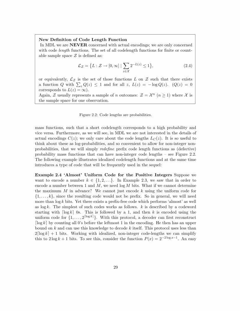
New Definition of Code Length FunctionIn MDL we are NEVER concerned with actual encodings; we are only concernedwith code length functions. The set of all codelength functions for finite or count-able sample space Z is defined as:

LZ ={

L : Z → [0,∞] |∑

z∈X

2−L(z) ≤ 1}

, (2.4)

or equivalently, LZ is the set of those functions L on Z such that there existsa function Q with

∑

z Q(z) ≤ 1 and for all z, L(z) = − logQ(z). (Q(z) = 0corresponds to L(z) =∞).Again, Z usually represents a sample of n outcomes: Z = X n (n ≥ 1) where X isthe sample space for one observation.

Figure 2.2: Code lengths are probabilities.

mass functions, such that a short codelength corresponds to a high probability andvice versa. Furthermore, as we will see, in MDL we are not interested in the details ofactual encodings C(z); we only care about the code lengths LC(z). It is so useful tothink about these as log-probabilities, and so convenient to allow for non-integer non-probabilities, that we will simply redefine prefix code length functions as (defective)probability mass functions that can have non-integer code lengths – see Figure 2.2.The following example illustrates idealized codelength functions and at the same timeintroduces a type of code that will be frequently used in the sequel:

Example 2.4 ‘Almost’ Uniform Code for the Positive Integers Suppose wewant to encode a number k ∈ {1, 2, . . .}. In Example 2.3, we saw that in order toencode a number between 1 and M , we need logM bits. What if we cannot determinethe maximum M in advance? We cannot just encode k using the uniform code for{1, . . . , k}, since the resulting code would not be prefix. So in general, we will needmore than log k bits. Yet there exists a prefix-free code which performs ‘almost’ as wellas log k. The simplest of such codes works as follows. k is described by a codewordstarting with dlog ke 0s. This is followed by a 1, and then k is encoded using theuniform code for {1, . . . , 2dlog ke}. With this protocol, a decoder can first reconstructdlog ke by counting all 0’s before the leftmost 1 in the encoding. He then has an upperbound on k and can use this knowledge to decode k itself. This protocol uses less than2dlog ke + 1 bits. Working with idealized, non-integer code-lengths we can simplifythis to 2 log k + 1 bits. To see this, consider the function P (x) = 2−2 log x−1. An easy

29

calculation gives

∑

x∈1,2,...

P (x) =∑

x∈1,2,...

2−2 log x−1 =1

2

∑

x∈1,2,...

x−2 <1

2+

1

2

∑

x=2,3,...

1

x(x− 1)= 1,

so that P is a (defective) probability distribution. Thus, by our new definition (Fig-ure 2.2), there exists a prefix code with, for all k, L(k) = − logP (k) = 2 log k + 1. Wecall the resulting code the ‘simple standard code for the integers’. In Section 2.5 wewill see that it is an instance of a so-called ‘universal’ code.

The idea can be refined to lead to codes with lengths log k+O(log log k); the ‘best’possible refinement, with code lengths L(k) increasing monotonically but as slowly aspossible in k, is known as ‘the universal code for the integers’ [Rissanen 1983]. However,for our purposes in this tutorial, it is good enough to encode integers k with 2 log k+1bits.

Example 2.5 [Example 1.2 and 2.2, Continued.] We are now also in a posi-tion to prove the third and final claim of Examples 1.2 and 2.2. Consider the threesequences (2.1), (2.2) and (2.3) on page 26 again. It remains to investigate howmuch the third sequence can be compressed. Assume for concreteness that, beforeseeing the sequence, we are told that the sequence contains a fraction of 1s equalto 1/5 + ε for some small unknown ε. By the Kraft inequality, Figure 2.1, for alldistributions P , there exists some code on sequences of length n such that for allxn ∈ Xn, L(xn) = d− logP (xn)e. The fact that the fraction of 1s is approximatelyequal to 1/5 suggests to model xn as independent outcomes of a coin with bias1/5-th. The corresponding distribution P0 satisfies

− logP0(xn) = log

(

1

5

)n[1](

4

5

)n[0]

= n[

−(1

5+ ε)

log1

5−(4

5− ε)

log4

5

]

=

n[log 5− 8

5+ 2ε],

where n[j] denotes the number of occurrences of symbol j in xn. For small enough ε,the part between brackets is smaller than 1, so that, using the code L0 with lengths− logP0, the sequence can be encoded using αn bits were α satisfies 0 < α < 1.Thus, using the code L0, the sequence can be compressed by a linear amount, ifwe use a specially designed code that assigns short codelengths to sequences withabout four times as many 0s than 1s.

We note that after the data (2.3) has been observed, it is always possible to designa code which uses arbitrarily few bits to encode xn - the actually observed sequencemay be encoded as ‘1’ for example, and no other sequence is assigned a codeword.The point is that with a code that has been designed before seeing the actualsequence, given only the knowledge that the sequence will contain approximatelyfour times as many 0s than 1s, the sequence is guaranteed to be compressed by anamount linear in n.

Continuous Sample Spaces How does the correspondence work for continuous-valued X ? In this tutorial we only consider P on X such that P admits a density5.

30

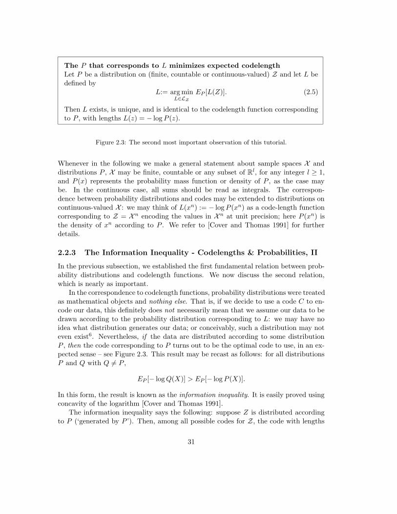
The P that corresponds to L minimizes expected codelengthLet P be a distribution on (finite, countable or continuous-valued) Z and let L bedefined by

L:= argminL∈LZ

EP [L(Z)]. (2.5)

Then L exists, is unique, and is identical to the codelength function correspondingto P , with lengths L(z) = − logP (z).

Figure 2.3: The second most important observation of this tutorial.

Whenever in the following we make a general statement about sample spaces X anddistributions P , X may be finite, countable or any subset of Rl, for any integer l ≥ 1,and P (x) represents the probability mass function or density of P , as the case maybe. In the continuous case, all sums should be read as integrals. The correspon-dence between probability distributions and codes may be extended to distributions oncontinuous-valued X : we may think of L(xn) := − logP (xn) as a code-length functioncorresponding to Z = X n encoding the values in X n at unit precision; here P (xn) isthe density of xn according to P . We refer to [Cover and Thomas 1991] for furtherdetails.

2.2.3 The Information Inequality - Codelengths & Probabilities, II

In the previous subsection, we established the first fundamental relation between prob-ability distributions and codelength functions. We now discuss the second relation,which is nearly as important.

In the correspondence to codelength functions, probability distributions were treatedas mathematical objects and nothing else. That is, if we decide to use a code C to en-code our data, this definitely does not necessarily mean that we assume our data to bedrawn according to the probability distribution corresponding to L: we may have noidea what distribution generates our data; or conceivably, such a distribution may noteven exist6. Nevertheless, if the data are distributed according to some distributionP , then the code corresponding to P turns out to be the optimal code to use, in an ex-pected sense – see Figure 2.3. This result may be recast as follows: for all distributionsP and Q with Q 6= P ,

EP [− logQ(X)] > EP [− logP (X)].

In this form, the result is known as the information inequality. It is easily proved usingconcavity of the logarithm [Cover and Thomas 1991].

The information inequality says the following: suppose Z is distributed accordingto P (‘generated by P ’). Then, among all possible codes for Z, the code with lengths

31

− logP (Z) ‘on average’ gives the shortest encodings of outcomes of P . Why shouldwe be interested in the average? The law of large numbers [Feller 1968] implies that,for large samples of data distributed according to P , with high P -probability, the codethat gives the shortest expected lengths will also give the shortest actual codelengths,which is what we are really interested in. This will hold if data are i.i.d., but also moregenerally if P defines a ‘stationary and ergodic’ process.

Example 2.6 Let us briefly illustrate this. Let P ∗, QA and QB be three proba-bility distributions on X , extended to Z = X n by independence. Hence P ∗(xn) =∏

P ∗(xi) and similarly for QA and QB . Suppose we obtain a sample generated byP ∗. Mr. A and Mrs. B both want to encode the sample using as few bits as possible,but neither knows that P ∗ has actually been used to generate the sample. A decidesto use the code corresponding to distribution QA and B decides to use the code cor-responding to QB . Suppose that EP∗ [− logQA(X)] < EP∗ [− logQB(X)]. Then,by the law of large numbers , with P ∗-probability 1, n−1[− logQj(X1, . . . , Xn)]→EP∗ [− logQj(X)], for both j ∈ {A,B} (note − logQj(X

n) = −∑n

i=1 logQj(Xi)).It follows that, with probability 1, Mr. A will need less (linearly in n) bits toencode X1, . . . , Xn than Mrs. B.

The qualitative content of this result is not so surprising: in a large sample generatedby P , the frequency of each x ∈ X will be approximately equal to the probabilityP (x). In order to obtain a short codelength for xn, we should use a code that assigns asmall codelength to those symbols in X with high frequency (probability), and a largecodelength to those symbols in X with low frequency (probability).

Summary and Outlook In this section we introduced (prefix) codes and thoroughlydiscussed the relation between probabilities and codelengths. We are now almost readyto formalize a simple version of MDL – but first we need to review some concepts ofstatistics.

2.3 Statistical Preliminaries and Example Models

In the next section we will make precise the crude form of MDL informally presentedin Section 1.3. We will freely use some convenient statistical concepts which we reviewin this section; for details see, for example, [Casella and Berger 1990]. We also describethe model class of Markov chains of arbitrary order, which we use as our runningexample. These admit a simpler treatment than the polynomials, to which we returnin Section 2.8.

Statistical Preliminaries A probabilistic model 7 M is a set of probabilistic sources.Typically one uses the word ‘model’ to denote sources of the same functional form. Weoften index the elements P of a model M using some parameter θ. In that case wewrite P as P (· | θ), and M as M = {P (· | θ) | θ ∈ Θ}, for some parameter space Θ. IfM can be parameterized by some connected Θ ⊆ Rk for some k ≥ 1 and the mapping

32

θ → P (· | θ) is smooth (appropriately defined), we callM a parametric model or family.For example, the modelM of all normal distributions on X = R is a parametric modelthat can be parameterized by θ = (µ, σ2) where µ is the mean and σ2 is the variance ofthe distribution indexed by θ. The family of all Markov chains of all orders is a model,but not a parametric model. We call a model M an i.i.d. model if, according to allP ∈M, X1, X2, . . . are i.i.d. We callM k-dimensional if k is the smallest integer k sothat M can be smoothly parameterized by some Θ ⊆ Rk.

For a given model M and sample D = xn, the maximum likelihood (ML) P isthe P ∈ M maximizing P (xn). For a parametric model with parameter space Θ, themaximum likelihood estimator θ is the function that, for each n, maps xn to the θ ∈ Θthat maximizes the likelihood P (xn | θ). The ML estimator may be viewed as a‘learning algorithm’. This is a procedure that, when input a sample xn of arbitrarylength, outputs a parameter or hypothesis Pn ∈ M. We say a learning algorithm isconsistent relative to distance measure d if for all P ∗ ∈ M, if data are distributedaccording to P ∗, then the output Pn converges to P ∗ in the sense that d(P ∗, Pn) → 0with P ∗-probability 1. Thus, if P ∗ is the ‘true’ state of nature, then given enough data,the learning algorithm will learn a good approximation of P ∗ with very high probability.

Example 2.7 [Markov and Bernoulli models] Recall that a k-th order Markovchain on X = {0, 1} is a probabilistic source such that for every n > k,

P (Xn = 1 | Xn−1 = xn−1, . . . , Xn−k = xn−k) =

P (Xn = 1 | Xn−1 = xn−1, . . . , Xn−k = xn−k, . . . , X1 = x1). (2.6)

That is, the probability distribution on Xn depends only on the k symbols preceding n.Thus, there are 2k possible distributions of Xn, and each such distribution is identifiedwith a state of the Markov chain. To fully identify the chain, we also need to specify thestarting state, defining the first k outcomes X1, . . . , Xk. The k-th order Markov modelis the set of all k-th order Markov chains, i.e. all sources satisfying (2.6) equipped witha starting state.

The special case of the 0-th order Markov model is the Bernoulli or biased coinmodel, which we denote by B(0) We can parameterize the Bernoulli model by a param-eter θ ∈ [0, 1] representing the probability of observing a 1. Thus, B(0) = {P (· | θ) | θ ∈[0, 1]}, with P (xn | θ) by definition equal to

P (xn | θ) =n∏

i=1

P (xi | θ) = θn[1](1− θ)n[0] ,

where n[1] stands for the number of 1s, and n[0] for the number of 0s in the sample.Note that the Bernoulli model is i.i.d. The log-likelihood is given by

logP (xn | θ) = n[1] log θ + n[0] log(1− θ). (2.7)

33

Taking the derivative of (2.7) with respect to θ, we see that for fixed xn, the log-likelihood is maximized by setting the probability of 1 equal to the observed frequency.Since the logarithm is a monotonically increasing function, the likelihood is maximizedat the same value: the ML estimator is given by θ(xn) = n[1]/n.

Similarly, the first-order Markov model B(1) can be parameterized by a vector θ =(θ[1|0], θ[1|1]) ∈ [0, 1]2 together with a starting state in {0, 1}. Here θ[1|j] represents theprobability of observing a 1 following the symbol j. The log-likelihood is given by

logP (xn | θ) = n[1|1] log θ[1|1] + n[0|1] log(1− θ[1|1]) + n[1|0] log θ[1|0] + n[0|0] log(1− θ[1|0]),

n[i|j] denoting the number of times outcome i is observed in state (previous outcome)

j. This is maximized by setting θ = (θ[1|0], θ[1|1]), with θ[i|j] = n[i|j] = n[ji]/n[j] set tothe conditional frequency of i preceded by j. In general, a k-th order Markov chain has2k parameters and the corresponding likelihood is maximized by setting the parameterθ[i|j] equal to the number of times i was observed in state j divided by the number oftimes the chain was in state j.

Suppose now we are given data D = xn and we want to find the Markov chain thatbest explains D. Since we do not want to restrict ourselves to chains of fixed order, werun a large risk of overfitting: simply picking, among all Markov chains of each order,the ML Markov chain that maximizes the probability of the data, we typically end upwith a chain of order n− 1 with starting state given by the sequence x1, . . . , xn−1, andP (Xn = xn | Xn−1 = xn−1) = 1. Such a chain will assign probability 1 to xn. Belowwe show that MDL makes a more reasonable choice.

2.4 Crude MDL

Based on the information-theoretic (Section 2.2) and statistical (Section 2.3) prelimi-naries discussed before, we now formalize a first, crude version of MDL.

LetM be a class of probabilistic sources (not necessarily Markov chains). Supposewe observe a sample D = (x1, . . . , xn) ∈ X n. Recall ‘the crude8 two-part code MDLPrinciple’ from Section 1.3, page 11:

Crude9, Two-part Version of MDL PrincipleLet H(1),H(2), . . . be a set of candidate models. The best point hypothesis H ∈H(1) ∪ H(2) ∪ . . . to explain data D is the one which minimizes the sum L(H) +L(D|H), where

• L(H) is the length, in bits, of the description of the hypothesis; and

• L(D|H) is the length, in bits, of the description of the data when encodedwith the help of the hypothesis.

The best model to explain D is the smallest model containing the selected H.

34

In this section, we implement this crude MDL Principle by giving a precise definitionof the terms L(H) and L(D|H). To make the first term precise, we must design acode C1 for encoding hypotheses H such that L(H) = LC1(H). For the second term,we must design a set of codes C2,H (one for each H ∈ M) such that for all D ∈ X n,L(D|H) = LC2,H

(D). We start by describing the codes C2,H .

2.4.1 Description Length of Data given Hypothesis

Given a sample of size n, each hypothesis H may be viewed as a probability distributionon X n. We denote the corresponding probability mass function by P (· | H). We needto associate with P (· | H) a code, or really, just a codelength function for X n. Wealready know that there exists a code with length function L such that for all xn ∈ X n,L(xn) = − logP (xn | H). This is the code that we will pick. It is a natural choice fortwo reasons:

1. With this choice, the code length L(xn | H) is equal to minus the log-likelihoodof xn according to H, which is a standard statistical notion of ‘goodness-of-fit’.

2. If the data turn out to be distributed according to P , then the code L(· | H) willuniquely minimize the expected code length (Section 2.2).

The second item implies that our choice is, in a sense, the only reasonable choice10.To see this, suppose M is a finite i.i.d. model containing, say, M distributions.Suppose we assign an arbitrary but finite code length L(H) to each H ∈M. Sup-pose X1, X2, . . . are actually distributed i.i.d. according to some ‘true’ H∗ ∈ M.By the reasoning of Example 2.6, we see that MDL will select the true distributionP (· | H∗) for all large n, with probability 1. This means that MDL is consistentfor finite M. If we were to assign codes to distributions in some other mannernot satisfying L(D | H) = − logP (D | H), then there would exist distributionsP (· | H) such that L(D|H) 6= − logP (D|H). But by Figure 2.1, there must besome distribution P (· | H ′) with L(·|H) = − logP (· | H ′). Now let M = {H,H ′}and suppose data are distributed according to P (· | H ′). Then, by the reasoningof Example 2.6, MDL would select H rather than H ′ for all large n! Thus, MDLwould be inconsistent even in this simplest of all imaginable cases – there wouldthen be no hope for good performance in the considerably more complex situationswe intend to use it for11.

2.4.2 Description Length of Hypothesis

In its weakest and crudest form, the two-part code MDL Principle does not give anyguidelines as to how to encode hypotheses (probability distributions). Every code forencoding hypotheses is allowed, as long as such a code does not change with the samplesize n.

To see the danger in allowing codes to depend on n, consider the Markov chainexample: if we were allowed to use different codes for different n, we could use, foreach n, a code assigning a uniform distribution to all Markov chains of order n− 1

35

with all parameters equal to 0 or 1. Since there are only a finite number (2n−1) ofthese, this is possible. But then, for each n, xn ∈ Xn, MDL would select the MLMarkov chain of order n− 1. Thus, MDL would coincide with ML and, no matterhow large n, we would overfit.

Consistency of Two-part MDL Remarkably, if we fix an arbitrary code for allhypotheses, identical for all sample sizes n, this is sufficient to make MDL consistent12

for a wide variety of models, including the Markov chains. For example, let L bethe length function corresponding to some code for the Markov chains. Suppose someMarkov chain P ∗ generates the data such that L(P ∗) < ∞ under our coding scheme.Then, broadly speaking, for every P ∗ of every order, with probability 1 there existssome n0 such that for all samples larger than n0, two-part MDL will select P ∗ – heren0 may depend on P ∗ and L.

While this results indicates that MDL may be doing something sensible, it certainlydoes not justify the use of arbitrary codes - different codes will lead to preferences ofdifferent hypotheses, and it is not at all clear how a code should be designed that leadsto good inferences with small, practically relevant sample sizes.

Barron and Cover [1991] have developed a precise theory of how to design codes C1

in a ‘clever’ way, anticipating the developments of ‘refined MDL’. Practitioners haveoften simply used ‘reasonable’ coding schemes, based on the following idea. Usuallythere exists some ‘natural’ decomposition of the models under consideration, M =⋃

k>0M(k) where the dimension of M(k) grows with k but is not necessarily equal to

k. In the Markov chain example, we have B =⋃B(k) where B(k) is the k-th order,

2k-parameter Markov model. Then within each submodel M(k), we may use a fixed-length code for θ ∈ Θ(k). Since the set Θ(k) is typically a continuum, we somehow needto discretize it to achieve this.

Example 2.8 [a Very Crude Code for the Markov Chains] We can describea Markov chain of order k by first describing k, and then describing a parametervector θ ∈ [0, 1]k

′with k′ = 2k. We describe k using our simple code for the integers

(Example 2.4). This takes 2 log k + 1 bits. We now have to describe the k′-componentparameter vector. We saw in Example 2.7 that for any xn, the best-fitting (ML) k-th order Markov chain can be identified with k′ frequencies. It is not hard to see thatthese frequencies are uniquely determined by the counts n[1|0...00], n[1|0...01], . . . , n[1|1...11].Each individual count must be in the (n+1)-element set {0, 1, . . . , n}. Since we assumen is given in advance13, we may use a simple fixed-length code to encode this count,taking log(n + 1) bits (Example 2.3). Thus, once k is fixed, we can describe such aMarkov chain by a uniform code using k′ log(n + 1) bits. With the code just definedwe get for any P ∈ B, indexed by parameter Θ(k),

L(P ) = L(k,Θ(k)) = 2 log k + 1 + k log(n+ 1),

so that with these codes, MDL tells us to pick the k, θ(k) minimizing

L(k, θ(k)) + L(D | k, θ(k)) = 2 log k + 1 + k log(n+ 1)− logP (D | k, θ(k)), (2.8)

36

where the θ(k) that is chosen will be equal to the ML estimator for M(k).

Why (not) this code? We may ask two questions about this code. First, why didwe only reserve codewords for θ that are potentially ML estimators for the given data?The reason is that, given k′ = 2k, the codelength L(D | k, θ(k)) is minimized by θ(k)(D),the ML estimator within θ(k). Reserving codewords for θ ∈ [0, 1]k

′that cannot be ML

estimates would only serve to lengthen L(D | k, θ(k)) and can never shorten L(k, θ(k)).Thus, the total description length needed to encode D will increase. Since our statedgoal is to minimize description lengths, this is undesirable.

However, by the same logic we may also ask whether we have not reserved too manycodewords for θ ∈ [0, 1]k

′

. And in fact, it turns out that we have: the distance betweentwo adjacent ML estimators is O(1/n). Indeed, if we had used a coarser precision, onlyreserving codewords for parameters with distances O(1/

√n), we would obtain smaller

code lengths - (2.8) would become

L(k, θ(k)) + L(D | k, θ(k)) = − logP (D | k, θ(k)) + k

2logn+ ck, (2.9)

where ck is a small constant depending on k, but not n [Barron and Cover 1991]. InSection 2.6 we show that (2.9) is in some sense ‘optimal’.

The Good News and the Bad News The good news is (1) we have found aprincipled, non-arbitrary manner to encode data D given a probability distributionH, namely, to use the code with lengths − logP (D | H); and (2), asymptotically,any code for hypotheses will lead to a consistent criterion. The bad news is that wehave not found clear guidelines to design codes for hypotheses H ∈ M. We foundsome intuitively reasonable codes for Markov chains, and we then reasoned that thesecould be somewhat ‘improved’, but what is conspicuously lacking is a sound theoreticalprinciple for designing and improving codes.

We take the good news to mean that our idea may be worth pursing further. Wetake the bad news to mean that we do have to modify or extend the idea to get ameaningful, non-arbitrary and practically relevant model selection method. Such anextension was already suggested in Rissanen’s early works [Rissanen 1978; Rissanen1983] and refined by Barron and Cover [1991]. However, in these works, the principlewas still restricted to two-part codes. To get a fully satisfactory solution, we need tomove to ‘universal codes’, of which the two-part codes are merely a special case.

2.5 Information Theory II: Universal Codes and Models

We have just indicated why the two-part code formulation of MDL needs to be refined.It turns out that the key concept we need is that of universal coding. Broadly speaking,a code L that is universal relative to a set of candidate codes L allows us to compressevery sequence xn almost as well as the code in L that compresses that particular

37

sequence most. Two-part codes are universal (Section 2.5.1), but there exist otheruniversal codes such as the Bayesian mixture code (Section 2.5.2) and the NormalizedMaximum Likelihood (NML) code (Section 2.5.3). We also discuss universal models,which are just the probability distributions corresponding to universal codes. In thissection, we are not concerned with learning from data; we only care about compressingdata as much as possible. We reconnect our findings with learning in Section 2.6.

Coding as Communication Like many other topics in coding, ‘universal coding’can best be explained if we think of descriptions as messages: we can always view adescription as a message that some sender or encoder, say Mr. A, sends to some receiveror decoder, say Mr. B. Before sending any messages, Mr. A and Mr. B meet in person.They agree on the set of messages that A may send to B. Typically, this will be the setX n of sequences x1, . . . , xn, where each xi is an outcome in the space X . They alsoagree upon a (prefix) code that will be used by A to send his messages to B. Once thishas been done, A and B go back to their respective homes and A sends his messagesto B in the form of binary strings. The unique decodability property of prefix codesimplies that, when B receives a message, he should always be able to decode it in aunique manner.

Universal Coding Suppose our encoder/sender is about to observe a sequence xn ∈X n which he plans to compress as much as possible. Equivalently, he wants to sendan encoded version of xn to the receiver using as few bits as possible. Sender andreceiver have a set of candidate codes L for X n available14. They believe or hope thatone of these codes will allow for substantial compression of xn. However, they mustdecide on a code for X n before sender observes the actual xn, and they do not knowwhich code in L will lead to good compression of the actual xn. What is the bestthing they can do? They may be tempted to try the following: upon seeing xn, sendersimply encodes/sends xn using the L ∈ L that minimizes L(xn) among all L ∈ L.But this naive scheme will not work: since decoder/receiver does not know what xn

has been sent before decoding the message, he does not know which of the codes inL has been used by sender/encoder. Therefore, decoder cannot decode the message:the resulting protocol does not constitute a uniquely decodable, let alone a prefix code.Indeed, as we show below, in general no code L exists such that for all xn ∈ X n,L(xn) ≤ minL∈L L(x

n): in words, there exists no code which, no matter what xn is,always mimics the best code for xn.

Example 2.9 Suppose we think that our sequence can be reasonably well-compressedby a code corresponding to some biased coin model. For simplicity, we restrict ourselvesto a finite number of such models. Thus, let L = {L1, . . . , L9} where L1 is the codelength function corresponding to the Bernoulli model P (· | θ) with parameter θ = 0.1,L2 corresponds to θ = 0.2 and so on. From (2.7) we see that, for example,

L8(xn) = − logP (xn|0.8) = −n[0] log 0.2− n[1] log 0.8

L9(xn) = − logP (xn|0.9) = −n[0] log 0.1− n[1] log 0.9.

38

Both L8(xn) and L9(x

n) are linearly increasing in the number of 1s in xn. However, ifthe frequency n1/n is approximately 0.8, then minL∈L L(x

n) will be achieved for L8. Ifn1/n ≈ 0.9 then minL∈L L(x

n) is achieved for L9. More generally, if n1/n ≈ j/10 thenLj achieves the minimum15. We would like to send xn using a code L such that forall xn, we need at most L(xn) bits, where L(xn) is defined as L(xn) := minL∈L L(x

n).Since − log is monotonically decreasing, L(xn) = − logP (xn | θ(xn)). We already gavean informal explanation as to why a code with lengths L does not exist. We can nowexplain this more formally as follows: if such a code were to exist, it would correspondto some distribution P . Then we would have for all xn, L(xn) = − log P (xn). But,by definition, for all xn ∈ X n, L(xn) ≤ L(xn) = − logP (xn|θ(xn)) where θ(xn) ∈{0.1, . . . , 0.9}. Thus we get for all xn, − log P (xn) ≤ − logP (xn | θ(xn)) or P (xn) ≥P (xn | θ(xn)), so that, since |L| > 1,

∑

xn

P (xn) ≥∑

xn

P (xn | θ(xn)) =∑

xn

maxθ

P (xn | θ) > 1, (2.10)

where the last inequality follows because for any two θ1, θ2 with θ1 6= θ2, there is atleast one xn with P (xn | θ1) > P (xn | θ2). (2.10) says that P is not a probabilitydistribution. It follows that L cannot be a codelength function. The argument canbe extended beyond the Bernoulli model of the example above: as long as |L| > 1,and all codes in L correspond to a non-defective distribution, (2.10) must still hold,so that there exists no code L with L(xn) = L(xn) for all xn. The underlying reasonthat no such code exists is the fact that probabilities must sum up to something ≤ 1;or equivalently, that there exists no coding scheme assigning short code words to manydifferent messages – see Example 2.2.

Since there exists no code which, no matter what xn is, always mimics the best code forxn, it may make sense to look for the next best thing: does there exist a code which,for all xn ∈ X n, is ‘nearly’ (in some sense) as good as L(xn)? It turns out that inmany cases, the answer is yes: there typically exists codes L such that no matter whatxn arrives, L(xn) is not much larger than L(xn), which may be viewed as the codethat is best ‘with hindsight’ (i.e., after seeing xn). Intuitively, codes which satisfy thisproperty are called universal codes - a more precise definition follows below. The first(but perhaps not foremost) example of a universal code is the two-part code that wehave encountered in Section 2.4.

2.5.1 Two-part Codes as simple Universal Codes

Example 2.10 [finite L] Let L be as in Example 2.9. We can devise a code L2-p

for all xn ∈ X n as follows: to encode xn, we first encode the j ∈ {1, . . . , 9} such thatLj(x

n) = minL∈L L(xn), using a uniform code. This takes log 9 bits. We then encode

xn itself using the code indexed by j. This takes Lj bits. Note that in contrast to thenaive scheme discussed in Example 2.9, the resulting scheme properly defines a prefixcode: a decoder can decode xn by first decoding j, and then decoding xn using Lj .

39

Thus, for every possible xn ∈ X n, we obtain

L2-p(xn) = min

L∈LL(xn) + log 9.

For all L ∈ L, minxn L(xn) grows linearly in n: minθ,xn − logP (xn | θ) = −n log 0.9 ≈

0.15n. Unless n is very small, no matter what xn arises, the extra number of bits weneed using L2-p compared to L(xn) is negligible.

More generally, let L = {L1, . . . , LM} where M can be arbitrarily large, and the Ljcan be any codelength functions we like; they do not necessarily represent Bernoullidistributions any more. By the reasoning of Example 2.10, there exists a (two-part)code such that for all xn ∈ X n,

L2-p(xn) = min

L∈LL(xn) + logM. (2.11)

In most applications minL(xn) grows linearly in n, and we see from (2.11) that, as soonas n becomes substantially larger than logM , the relative difference in performancebetween our universal code and L(xn) becomes negligible. In general, we do not alwayswant to use a uniform code for the elements in L; note that any arbitrary code on Lwill give us an analogue of (2.11), but with a worst-case overhead larger than logM -corresponding to the largest codelength of any of the elements in L.

Example 2.11 [Countably Infinite L] We can also construct a 2-part code for ar-bitrary countably infinite sets of codes L = {L1, L2, . . .}: we first encode some k usingour simple code for the integers (Example 2.4). With this code we need 2 log k+1 bitsto encode integer k. We then encode xn using the code Lk. L2-p is now defined as thecode we get if, for any xn, we encode xn using the Lk minimizing the total two-partdescription length 2 log k + 1 + Lk(x

n).In contrast to the case of finite L, there does not exist a constant c any more such

that for all n, xn ∈ X n, L2-p(xn) ≤ infL∈L L(x

n) + c. Instead we have the followingweaker, but still remarkable property: for all k, all n, all xn, L2-p(x

n) ≤ Lk(xn) +

2 log k + 1, so that also,

L2-p(xn) ≤ inf

L∈{L1,...,Lk}L(xn) + 2 log k + 1.

For any k, as n grows larger, the code L2-p starts to mimic whatever L ∈ {L1, . . . , Lk}compresses the data most. However, the larger k, the larger n has to be before thishappens.

2.5.2 From Universal Codes to Universal Models

Instead of postulating a set of candidate codes L, we may equivalently postulate a setM of candidate probabilistic sources, such that L is the set of codes corresponding toM. We already implicitly did this in Example 2.9.

40

The reasoning is now as follows: we think that one of the P ∈M will assign a highlikelihood to the data to be observed. Therefore we would like to design a code that,for all xn we might observe, performs essentially as well as the code corresponding tothe best-fitting, maximum likelihood (minimum codelength) P ∈ M for xn. Similarly,we can think of universal codes such as the two-part code in terms of the (possiblydefective, see Section 2.2 and Figure 2.1)) distributions corresponding to it. Suchdistributions corresponding to universal codes are called universal models. The use ofmapping universal codes back to distributions is illustrated by the Bayesian universalmodel which we now introduce.

Universal model: Twice Misleading Terminology The words ‘universal’ and‘model’ are somewhat of a misnomer: first, these codes/models are only ‘universal’relative to a restricted ‘universe’ M. Second, the use of the word ‘model’ will bevery confusing to statisticians, who (as we also do in this paper) call a family ofdistributions such as M a ’model’. But the phrase originates from informationtheory, where a ‘model’ often refers to a single distribution rather than a family.Thus, a ‘universal model’ is a single distribution, representing a statistical ‘model’M.

Example 2.12 [Bayesian Universal Model] Let M be a finite or countable set ofprobabilistic sources, parameterized by some parameter set Θ. Let W be a distributionon Θ. Adopting terminology from Bayesian statistics, W is usually called a priordistribution. We can construct a new probabilistic source PBayes by taking a weighted(according to W ) average or mixture over the distributions in M. That is, we definefor all n, xn ∈ X ,

PBayes(xn) :=

∑

θ∈Θ

P (xn | θ)W (θ). (2.12)

It is easy to check that PBayes is a probabilistic source according to our definition.In case Θ is continuous, the sum gets replaced by an integral but otherwise nothingchanges in the definition. In Bayesian statistics, PBayes is called the Bayesian marginallikelihood or Bayesian mixture [Bernardo and Smith 1994]. To see that PBayes is auniversal model, note that for all θ0 ∈ Θ,

− log PBayes(xn) := − log

∑

θ∈Θ

P (xn | θ)W (θ) ≤ − logP (xn | θ0) + cθ0 (2.13)

where the inequality follows because a sum is at least as large as each of its terms,and cθ = − logW (θ) depends on θ but not on n. Thus, PBayes is a universal modelor equivalently, the code with lengths − log PBayes is a universal code. Note that thederivation in (2.13) only works if Θ is finite or countable; the case of continuous Θ istreated in Section 2.6.

Bayes is Better than Two-part The Bayesian model is in a sense superior to thetwo-part code. Namely, in the two-part code we first encode an element of M or its

41

parameter set Θ using some code L0. Such a code must correspond to some ‘prior’distribution W on M so that the two-part code gives codelengths

L2-p(xn) = min

θ∈Θ− logP (xn|θ)− logW (θ) (2.14)

where W depends on the specific code L0 that was used. Using the Bayes code withprior W , we get as in (2.13),

− log PBayes(xn) = − log

∑

θ∈Θ

P (xn | θ)W (θ) ≤ minθ∈Θ

− logP (xn|θ)− logW (θ).

The inequality becomes strict whenever P (xn|θ) > 0 for more than one value of θ.Comparing to (2.14), we see that in general the Bayesian code is preferable over thetwo-part code: for all xn it never assigns codelengths larger than L2-p(x

n), and in manycases it assigns strictly shorter codelengths for some xn. But this raises two importantissues: (1) what exactly do we mean by ‘better’ anyway? (2) can we say that ‘someprior distributions are better than others’? These questions are answered below.

2.5.3 NML as an Optimal Universal Model

We can measure the performance of universal models relative to a set of candidatesources M using the regret :

Definition 2.13 [Regret] LetM be a class of probabilistic sources. Let P be a prob-ability distribution on X n (P is not necessarily in M). For given xn, the regret of Prelative toM is defined as

− log P (xn)− minP∈M

{− logP (xn)}. (2.15)

The regret of P relative toM for xn is the additional number of bits needed to encodexn using the code/distribution P , as compared to the number of bits that had beenneeded if we had used code/distribution in M that was optimal (‘best-fitting’) withhind-sight. For simplicity, from now on we tacitly assume that for all the models Mwe work with, there is a single θ(xn) maximizing the likelihood for every xn ∈ X n. Inthat case (2.15) simplifies to

− log P (xn)− {− logP (xn | θ(xn))}.

We would like to measure the quality of a universal model P in terms of its regret.However, P may have small (even < 0) regret for some xn, and very large regret forother xn. We must somehow find a measure of quality that takes into account allxn ∈ X n. We take a worst-case approach, and look for universal models P with smallworst-case regret, where the worst-case is over all sequences. Formally, the maximumor worst-case regret of P relative to M is defined as

Rmax(P ):= maxxn∈Xn

{

− log P (xn)− {− logP (xn | θ(xn))}}

.

42

If we use Rmax as our quality measure, then the ‘optimal’ universal model relative toM, for given sample size n, is the distribution minimizing

minP

Rmax(P ) = minP

maxxn∈Xn

{

− log P (xn)− {− logP (xn | θ(xn))}}

(2.16)

where the minimum is over all defective distributions on X n. The P minimizing (2.16)corresponds to the code minimizing the additional number of bits compared to code inM that is best in hindsight in the worst-case over all possible xn. It turns out that wecan solve for P in (2.16). To this end, we first define the complexity of a given modelM as

COMPn(M):= log∑

xn∈Xn

P (xn | θ(xn)). (2.17)

This quantity plays a fundamental role in refined MDL, Section 2.6. To get a first ideaof why COMPn is called model complexity, note that the more sequences xn withlarge P (xn | θ(xn)), the larger COMPn(M). In other words, the more sequences thatcan be fit well by an element of M, the larger M’s complexity.

Proposition 2.14 [Shtarkov 1987] Suppose that COMPn(M) is finite. Then theminimax regret (2.16) is uniquely achieved for the distribution Pnml given by

Pnml(xn):=

P (xn | θ(xn))∑

yn∈Xn P (yn | θ(yn)). (2.18)

The distribution Pnml is known as the Shtarkov distribution or the normalized maximumlikelihood (NML) distribution.

Proof Plug in Pnml in (2.16) and notice that for all xn ∈ X n,

− log P (xn)− {− logP (xn | θ(xn))} = Rmax(P ) = COMPn(M), (2.19)

so that Pnml achieves the same regret, equal to COMPn(M), no matter what xn

actually obtains. Since every distribution P on X n with P 6= Pnml must satisfy P (zn) <Pnml(z

n) for at least one zn ∈ X n, it follows that

Rmax(P ) ≥ − logP (zn) + logP (zn | θ(zn)) >− log Pnml(z

n) + logP (zn | θ(zn)) = Rmax(Pnml).

2

Pnml is quite literally a ‘normalized maximum likelihood’ distribution: it tries to assignto each xn the probability of xn according to the ML distribution for xn. By (2.10),this is not possible: the resulting ‘probabilities’ add to something larger than 1. Butwe can normalize these ‘probabilities’ by dividing by their sum

∑

yn∈Xn P (yn | θ(yn)),and then we obtain a probability distribution on X n after all.

43

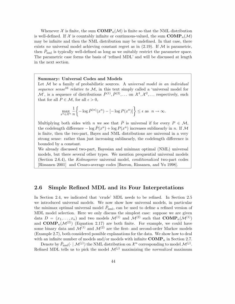
Whenever X is finite, the sum COMPn(M) is finite so that the NML distributionis well-defined. If X is countably infinite or continuous-valued, the sum COMPn(M)may be infinite and then the NML distribution may be undefined. In that case, thereexists no universal model achieving constant regret as in (2.19). If M is parametric,then Pnml is typically well-defined as long as we suitably restrict the parameter space.The parametric case forms the basis of ‘refined MDL’ and will be discussed at lengthin the next section.

Summary: Universal Codes and ModelsLet M be a family of probabilistic sources. A universal model in an individualsequence sense16 relative to M, in this text simply called a ‘universal model forM’, is a sequence of distributions P (1), P (2), . . . on X 1,X 2, . . . respectively, suchthat for all P ∈M, for all ε > 0,

maxxn∈Xn

1

n

{

− log P (n)(xn)− [− logP (xn)]

}

≤ ε as n→∞.

Multiplying both sides with n we see that P is universal if for every P ∈ M,the codelength difference − log P (xn) + logP (xn) increases sublinearly in n. If Mis finite, then the two-part, Bayes and NML distributions are universal in a verystrong sense: rather than just increasing sublinearly, the codelength difference isbounded by a constant.We already discussed two-part, Bayesian and minimax optimal (NML) universalmodels, but there several other types. We mention prequential universal models(Section 2.6.4), the Kolmogorov universal model, conditionalized two-part codes[Rissanen 2001] and Cesaro-average codes [Barron, Rissanen, and Yu 1998].

2.6 Simple Refined MDL and its Four Interpretations

In Section 2.4, we indicated that ‘crude’ MDL needs to be refined. In Section 2.5we introduced universal models. We now show how universal models, in particularthe minimax optimal universal model Pnml, can be used to define a refined version ofMDL model selection. Here we only discuss the simplest case: suppose we are givendata D = (x1, . . . , xn) and two models M(1) and M(2) such that COMPn(M(1))and COMPn(M(2)) (Equation 2.17) are both finite. For example, we could havesome binary data and M(1) and M(2) are the first- and second-order Markov models(Example 2.7), both considered possible explanations for the data. We show how to dealwith an infinite number of models and/or models with infinite COMPn in Section 2.7.

Denote by Pnml(· | M(j)) the NML distribution on X n corresponding to modelM(j).Refined MDL tells us to pick the model M(j) maximizing the normalized maximum

44

likelihood Pnml(D | M(j)), or, by (2.18), equivalently, minimizing

− log Pnml(D | M(j)) = − logP (D | θ(j)(D)) +COMPn(M(j)) (2.20)

From a coding theoretic point of view, we associate with eachM(j) a code with lengthsPnml(· | M(j)), and we pick the model minimizing the codelength of the data. Thecodelength − log Pnml(D | M(j)) has been called the stochastic complexity of the dataD relative to modelM(j) [Rissanen 1987], whereas COMPn(M(j)) is called the para-metric complexity or model cost ofM(j) (in this survey we simply call it ‘complexity’).We have already indicated in the previous section that COMPn(M(j)) measures some-thing like the ‘complexity’ of model M(j). On the other hand, − logP (D | θ(j)(D)) isminus the maximized log-likelihood of the data, so it measures something like (minus)fit or error – in the linear regression case, it can be directly related to the mean squarederror, Section 2.8. Thus, (2.20) embodies a trade-off between lack of fit (measured byminus log-likelihood) and complexity (measured by COMPn(M(j))). The confidencein the decision is given by the codelength difference

∣

∣

∣

∣

− log Pnml(D | M(1))− [− log Pnml(D | M(2))]

∣

∣

∣

∣

.

In general, − log Pnml(D | M) can only be evaluated numerically – the only exceptionthis author is aware of is whenM is the Gaussian family, Example 2.20. In many caseseven numerical evaluation is computationally problematic. But the re-interpretationsof Pnml we provide below also indicate that in many cases, − log P (D | M) is relativelyeasy to approximate.

Example 2.15 [Refined MDL and GLRT] Generalized likelihood ratio testing[Casella and Berger 1990] tells us to pick the M(j) maximizing logP (D | θ(j)(D)) +c where c is determined by the desired type-I and type-II errors. In practice oneoften applies a naive variation17, simply picking the modelM(j) maximizing logP (D |θ(j)(D)). This amounts to ignoring the complexity terms COMPn(M(j)) in (2.20):MDL tries to avoid overfitting by picking the model maximizing the normalized ratherthan the ordinary likelihood. The more distributions in M that fit the data well, thelarger the normalization term.

The hope is that the normalization term COMPn(M(j)) strikes the right balancebetween complexity and fit. Whether it really does depends on whether COMPn isa ‘good’ measure of complexity. In the remainder of this section we shall argue thatit is, by giving four different interpretations of COMPn and of the resulting trade-off(2.20):

1. Compression interpretation.

2. Counting interpretation.

3. Bayesian interpretation.

4. Prequential (predictive) interpretation.

45

2.6.1 Compression Interpretation

Rissanen’s original goal was to select the model that detects the most regularity inthe data; he identified this with the ‘model that allows for the most compression ofdata xn’. To make this precise, a code is associated with each model. The NML codewith lengths − log Pnml(· | M(j)) seems to be a very reasonable choice for such a codebecause of the following two properties:

1. The better the best-fitting distribution in M(j) fits the data, the shorter thecodelength − log Pnml(D | M(j)).

2. No distribution in M(j) is given a prior preference over any other distribution,since the regret of Pnml(· | M(j)) is the same for all D ∈ X n (Equation (2.19)).Pnml is the only complete prefix code with this property, which may be restatedas: Pnml treats all distributions within eachM(j) on the same footing!

Therefore, if one is willing to accept the basic ideas underlying MDL as first principles,then the use of NML in model selection is now justified to some extent. Below we giveadditional justifications that are not directly based on data compression; but we firstprovide some further interpretation of − log Pnml.

Compression and Separating Structure from Noise We present the followingideas in an imprecise fashion – Rissanen and Tabus [2004] recently showed how tomake them precise. The stochastic complexity of data D relative to M, given by(2.20) can be interpreted as the amount of information in the data relative to M,measured in bits. Although a one-part codelength, it still consists of two terms: a termCOMPn(M) measuring the amount of structure ormeaningful information in the data(as ‘seen through M’), and a term − logP (D | θ(D)) measuring the amount of noiseor accidental information in the data. To see that this second term measures noise,consider the regression example, Example 1.2, again. As will be seen in Section 2.8,Equation (2.40), in that case − logP (D | θ(D)) becomes equal to a linear function of themean squared error of the best-fitting polynomial in the set of k-th degree polynomials.To see that the first term measures structure, we reinterpret it below as the number ofbits needed to specify a ‘distinguishable’ distribution in M, using a uniform code onall ‘distinguishable’ distributions.

2.6.2 Counting Interpretation

The parametric complexity can be interpreted as measuring (the log of) the number ofdistinguishable distributions in the model. Intuitively, the more distributions a modelcontains, the more patterns it can fit well so the larger the risk of overfitting. However,if two distributions are very ‘close’ in the sense that they assign high likelihood to thesame patterns, they do not contribute so much to the complexity of the overall model.It seems that we should measure complexity of a model in terms of the number ofdistributions it contains that are ‘essentially different’ (distinguishable), and we now

46

show that COMPn measures something like this. Consider a finite model M withparameter set Θ = {θ1, . . . , θM}. Note that

∑

xn∈Xn

P (xn|θ(xn)) =∑

j=1..M

∑

xn:θ(xn)=θj

P (xn|θj) =

∑

j=1..M

(

1−∑

xn:θ(xn)6=θj

P (xn|θj))

= M −∑

j

P (θ(xn) 6= θj |θj).

We may think of P (θ(xn) 6= θj |θj) as the probability, according to θj , that the datalook as if they come from some θ 6= θj . Thus, it is the probability that θj is mistaken foranother distribution in Θ. Therefore, for finite M, Rissanen’s model complexity is thelogarithm of the number of distributions minus the summed probability that some θj is‘mistaken’ for some θ 6= θj . Now supposeM is i.i.d. By the law of large numbers [Feller

1968], we immediately see that the ‘sum of mistake probabilities’∑

j P (θ(xn) 6= θj |θj)tends to 0 as n grows. It follows that for large n, the model complexity converges tologM . For large n, the distributions inM are ‘perfectly distinguishable’ (the probabil-ity that a sample coming from one is more representative of another is negligible), andthen the parametric complexity COMPn(M) ofM is simply the log of the number ofdistributions in M.

Example 2.16 [NML vs. Two-part Codes] Incidentally, this shows that for finitei.i.d. M, the two-part code with uniform prior W on M is asymptotically minimaxoptimal: for all n, the regret of the 2-part code is logM (Equation 2.11), whereas wejust showed that for n→∞, R(Pnml) = COMPn(M)→ logM . However, for small n,some distributions inMmay be mistaken for one another; the number of distinguishabledistributions in M is then smaller than the actual number of distributions, and this isreflected in COMPn(M) being (sometimes much) smaller than logM .

For the more interesting case of parametric models, containing infinitely many distribu-tions, Balasubramanian [1997, 2004] has a somewhat different counting interpretationof COMPn(M) as a ratio between two volumes. Rissanen and Tabus [2004] give amore direct counting interpretation of COMPn(M). These extensions are both basedon the asymptotic expansion of Pnml, which we now discuss.

Asymptotic Expansion of Pnml and COMPn Let M be a k-dimensional para-metric model. Under regularity conditions onM and the parameterization Θ→M, tobe detailed below, we obtain the following asymptotic expansion of COMPn [Rissanen1996; Takeuchi and Barron 1997; Takeuchi and Barron 1998; Takeuchi 2000]:

COMPn(M) =k

2log

n

2π+ log

∫

θ∈Θ

√

|I(θ)|dθ + o(1). (2.21)

Here k is the number of parameters (degrees of freedom) in model M, n is the samplesize, and o(1)→ 0 as n→∞. |I(θ)| is the determinant of the k×k Fisher information

47

matrix18 I evaluated at θ. In case M is an i.i.d. model, I is given by

Iij(θ∗):=Eθ∗

{

− ∂2

∂θi∂θjlogP (X|θ)

}

θ=θ∗.

This is generalized to non-i.i.d. models as follows:

Iij(θ∗):= lim

n→∞

1

nEθ∗

{

− ∂2

∂θi∂θjlogP (Xn|θ)

}

θ=θ∗.

(2.21) only holds if the model M, its parameterization Θ and the sequence x1, x2, . . .all satisfy certain conditions. Specifically, we require:

1. COMPn(M) <∞ and∫√

|I(θ)|dθ <∞;

2. θ(xn) does not come arbitrarily close to the boundary of Θ: for some ε > 0, forall large n, θ(xn) remains farther than ε from the boundary of Θ.

3. M and Θ satisfy certain further conditions. A simple sufficient condition is thatM be an exponential family [Casella and Berger 1990]. Roughly, this is a familythat can be parameterized so that for all x, P (x | β) = exp(βt(x))f(x)g(β),where t : X → R is a function of X. The Bernoulli model is an exponentialfamily, as can be seen by setting β := ln(1 − θ) − ln θ and t(x) = x. Alsothe multinomial, Gaussian, Poisson, Gamma, exponential, Zipf and many othermodels are exponential families; but, for example, mixture models are not.

More general conditions are given by Takeuchi and Barron [1997, 1998, 2000]. Essen-tially, if M behaves ‘asymptotically’ like an exponential family, then (2.21) still holds.For example, (2.21) holds for the Markov models and for AR and ARMA processes.

Example 2.17 [Complexity of the Bernoulli Model] The Bernoulli model B(0)

can be parameterized in a 1-1 way by the unit interval (Example 2.7). Thus, k = 1.An easy calculation shows that the Fisher information is given by θ(1 − θ). Pluggingthis into (2.21) and calculating

∫√

|θ(1− θ)|dθ gives

COMPn(B(0)) =1

2log n+

1

2log

π

2− 3 + o(1) =

1

2logn− 2.674251935 + o(1).

Computing the integral of the Fisher determinant is not easy in general. Hanson andFu [2004] compute it for several practically relevant models.

Whereas for finite M, COMPn(M) remains finite, for parametric models it generallygrows logarithmically in n. Since typically − logP (xn | θ(xn)) grows linearly in n, it isstill the case that for fixed dimensionality k (i.e. for a fixed M that is k-dimensional)and large n, the part of the codelength − log Pnml(x

n | M) due to the complexity ofM is very small compared to the part needed to encode data xn with θ(xn). The term∫

Θ

√

|I(θ)|dθ may be interpreted as the contribution of the functional form of M to

48

the model complexity [Balasubramanian 2004]. It does not grow with n so that, whenselecting between two models, it becomes irrelevant and can be ignored for very largen. But for small n, it can be important, as can be seen from Example 1.4, Fechner’sand Stevens’ model. Both models have two parameters, yet the

∫

Θ

√

|I(θ)|dθ-term ismuch larger for Fechner’s than for Stevens’ model. In the experiments of Myung, Bala-subramanian, and Pitt [2000], the parameter set was restricted to 0 < a <∞, 0 < b < 3for Stevens’ model and 0 < a <∞, 0 < b <∞ for Fechner’s model. The variance of theerror Z was set to 1 in both models. With these values, the difference in

∫

Θ

√

|I(θ)|dθis 3.804, which is non-negligible for small samples. Thus, Stevens’ model contains moredistinguishable distributions than Fechner’s, and is better able to capture random noisein the data – as Townsend [1975] already speculated almost 30 years ago. Experimentssuggest that for regression models such as Stevens’ and Fechner’s’, as well as for Markovmodels and general exponential families, the approximation (2.21) is reasonably accu-rate already for small samples. But this is certainly not true for general models:

The Asymptotic Expansion of COMPn Should Be Used with Care!(2.21) does not hold for all parametric models; and for some models for which itdoes hold, the o(1) term may only converge to 0 only for quite large sample sizes.Foster and Stine [1999, 2004] show that the approximation (2.21) is, in general,only valid if k is much smaller than n.

Two-part codes and COMPn(M) We now have a clear guiding principle (mini-max regret) which we can use to construct ‘optimal’ two-part codes, that achieve theminimax regret among all two-part codes. How do such optimal two-part codes compareto the NML codelength? Let M be a k-dimensional model. By slightly adjusting thearguments of [Barron and Cover 1991, Appendix], one can show that, under regularityconditions, the minimax optimal two-part code P2-p achieves regret

− log P2-p(xn | M) + logP (xn | θ(xn)) = k

2log

n

2π+ log

∫

θ∈Θ

√

|I(θ)|dθ + f(k) + o(1),

where f : N → R is a bounded positive function satisfying limk→∞ f(k) = 0. Thus, forlarge k, optimally designed two-part codes are about as good as NML. The problemwith two-part code MDL is that in practice, people often use much cruder codes withmuch larger minimax regret.

2.6.3 Bayesian Interpretation

The Bayesian method of statistical inference provides several alternative approaches tomodel selection. The most popular of these is based on Bayes factors [Kass and Raftery1995]. The Bayes factor method is very closely related to the refined MDL approach.Assuming uniform priors on modelsM(1) andM(2), it tells us to select the model with

49

largest marginal likelihood PBayes(xn | M(j)), where PBayes is as in (2.12), with the sum

replaced by an integral, and w(j) is the density of the prior distribution on M(j):

PBayes(xn | M(j)) =

∫

P (xn | θ)w(j)(θ)dθ. (2.22)

M is Exponential Family Let now PBayes = PBayes(· | M) for some fixed modelM. Under regularity conditions on M, we can perform a Laplace approximation ofthe integral in (2.12). For the special case that M is an exponential family, we obtainthe following expression for the regret [Jeffreys 1961; Schwarz 1978; Kass and Raftery1995; Balasubramanian 1997]:

− log PBayes(xn)− [− logP (xn | θ(xn))] = k

2log

n

2π− logw(θ) + log

√

|I(θ)|+ o(1).

(2.23)Let us compare this with (2.21). Under the regularity conditions needed for (2.21), thequantity on the right of (2.23) is within O(1) of COMPn(M). Thus, the code lengthachieved with PBayes is within a constant of the minimax optimal − log Pnml(x

n). Since

− logP (xn | θ(xn)) increases linearly in n, this means that if we compare two modelsM(1) and M(2), then for large enough n, Bayes and refined MDL select the samemodel. If we equip the Bayesian universal model with a special prior known as theJeffreys-Bernardo prior [Jeffreys 1946; Bernardo and Smith 1994],

wJeffreys(θ) =

√

|I(θ)|∫

θ∈Θ

√

|I(θ)|dθ, (2.24)

then Bayes and refined NML become even more closely related: plugging in (2.24) into(2.23), we find that the right-hand side of (2.23) now simply coincides with (2.21). Aconcrete example of Jeffreys’ prior is given in Example 2.19. Jeffreys introduced hisprior as a ‘least informative prior’, to be used when no useful prior knowledge aboutthe parameters is available [Jeffreys 1946]. As one may expect from such a prior, itis invariant under continuous 1-to-1 reparameterizations of the parameter space. Thepresent analysis shows that, when M is an exponential family, then it also leads toasymptotically minimax codelength regret: for large n, refined NML model selectionbecomes indistinguishable from Bayes factor model selection with Jeffreys’ prior.

M is not an Exponential Family Under weak conditions on M, Θ and the se-quence xn, we get the following generalization of (2.23):

− log PBayes(xn | M) =

− logP (xn | θ(xn)) + k

2log

n

2π− logw(θ) + log

√

∣

∣I(xn)∣

∣+ o(1). (2.25)

Here I(xn) is the so-called observed information, sometimes also called observed Fisherinformation; see [Kass and Voss 1997] for a definition. If M is an exponential family,

50

then the observed Fisher information at xn coincides with the Fisher information atθ(xn), leading to (2.23). IfM is not exponential, then if data are distributed accordingto one of the distributions in M, the observed Fisher information still converges withprobability 1 to the expected Fisher information. If M is neither exponential, norare the data actually generated by a distribution in M, then there may be O(1)-discrepancies between − log Pnml and − log PBayes even for large n.

2.6.4 Prequential Interpretation

Distributions as Prediction Strategies Let P be a distribution on X n. Applyingthe definition of conditional probability, we can write for every xn:

P (xn) =n∏

i=1

P (xi)

P (xi−1)=

n∏

i=1

P (xi | xi−1), (2.26)

so that also

− logP (xn) =n∑

i=1

− logP (xi | xi−1) (2.27)

Let us abbreviate P (Xi = · | X i−1 = xi−1) to P (Xi | xi−1). P (Xi | xi−1) (capitalXi) is the distribution (not a single number) of Xi given xi−1; P (xi | xi−1) (lower casexi) is the probability (a single number) of actual outcome xi given xi−1. We can thinkof − logP (xi | xi−1) as the loss incurred when predicting Xi based on the conditionaldistribution P (Xi | xi−1), and the actual outcome turned out to be xi. Here ‘loss’ ismeasured using the so-called logarithmic score, also known simply as ‘log loss’. Notethat the more likely x is judged to be, the smaller the loss incurred when x actuallyobtains. The log loss has a natural interpretation in terms of sequential gambling [Coverand Thomas 1991], but its main interpretation is still in terms of coding: by (2.27),the codelength needed to encode xn based on distribution P is just the accumulated logloss incurred when P is used to sequentially predict the i-th outcome based on the past(i− 1)-st outcomes.

(2.26) gives a fundamental re-interpretation of probability distributions as predic-tion strategies, mapping each individual sequence of past observations x1, . . . , xi−1 to aprobabilistic prediction of the next outcome P (Xi | xi−1). Conversely, (2.26) also showsthat every probabilistic prediction strategy for sequential prediction of n outcomes maybe thought of as a probability distribution on X n: a strategy is identified with a functionmapping all potential initial segments xi−1 to the prediction that is made for the nextoutcome Xi, after having seen xi−1. Thus, it is a function S : ∪0≤i<nX i → PX , wherePX is the set of distributions on X . We can now define, for each i < n, all xi ∈ X i,P (Xi | xi−1):=S(xi−1). We can turn these partial distributions into a distribution onX n by sequentially plugging them into (2.26).

Log Loss for Universal Models Let M be some parametric model and let Pbe some universal model/code relative to M. What do the individual predictions

51

P (Xi | xi−1) look like? Readers familiar with Bayesian statistics will realize thatfor i.i.d. models, the Bayesian predictive distribution PBayes(Xi | xi−1) converges to

the ML distribution P (· | θ(xi−1)); Example 2.19 provides a concrete case. It seemsreasonable to assume that something similar holds not just for PBayes but for universalmodels in general. This in turn suggests that we may approximate the conditionaldistributions P (Xi | xi−1) of any ‘good’ universal model by the maximum likelihoodpredictions P (· | θ(xi−1)). Indeed, we can recursively define the ‘maximum likelihoodplug-in’ distribution Pplug-in by setting, for i = 1 to n,

Pplug-in(Xi = · | xi−1):=P (X = · | θ(xi−1)). (2.28)

Then

− log Pplug-in(xn):=

n∑

i=1

− logP (xi | θ(xi−1)). (2.29)

Indeed, it turns out that under regularity conditions on M and xn,

− log Pplug-in(xn) = − logP (xn | θ(xn)) + k

2log n+O(1), (2.30)

showing that Pplug-in acts as a universal model relative to M, its performance beingwithin a constant of the minimax optimal Pnml. The construction of Pplug-in can beeasily extended to non-i.i.d. models, and then, under regularity conditions, (2.30) stillholds; we omit the details.

We note that all general proofs of (2.30) that we are aware of show that (2.30) holdswith probability 1 or in expectation for sequences generated by some distributionin M [Rissanen 1984; Rissanen 1986; Rissanen 1989]. Note that the expressions(2.21) and (2.25) for the regret of Pnml and PBayes hold for a much wider classof sequences; they also hold with probability 1 for i.i.d. sequences generated bysufficiently regular distributions outside M. Not much is known about the regretobtained by Pplug-in for such sequences, except for some special cases such as ifMis the Gaussian model.

In general, there is no need to use the ML estimator θ(xi−1) in the definition (2.28).Instead, we may try some other estimator which asymptotically converges to the MLestimator – it turns out that some estimators considerably outperform the ML estima-tor in the sense that (2.29) becomes a much better approximation of − log Pnml, seeExample 2.19. Irrespective of whether we use the ML estimator or something else,we call model selection based on (2.29) the prequential form of MDL in honor of A.P.Dawid’s ‘prequential analysis’, Section 2.9. It is also known as ‘predictive MDL’. Thevalidity of (2.30) was discovered independently by Rissanen [1984] and Dawid [1984].

The prequential view gives us a fourth interpretation of refined MDL model selec-tion: given modelsM(1) andM(2), MDL tells us to pick the model that minimizes theaccumulated prediction error resulting from sequentially predicting future outcomesgiven all the past outcomes.

52

Example 2.18 [GLRT and Prequential Model Selection] How does this differfrom the naive version of the generalized likelihood ratio test (GLRT) that we intro-duced in Example 2.15? In GLRT, we associate with each model the log-likelihood(minus log loss) that can be obtained by the ML estimator. This is the predictorwithin the model that minimizes log loss with hindsight, after having seen the data.In contrast, prequential model selection associates with each model the log-likelihood(minus log loss) that can be obtained by using a sequence of ML estimators θ(xi−1)to predict data xi. Crucially, the data on which ML estimators are evaluated has notbeen used in constructing the ML estimators themselves. This makes the predictionscheme ‘honest’ (different data are used for training and testing) and explains why itautomatically protects us against overfitting.

Example 2.19 [Laplace and Jeffreys] Consider the prequential distribution for theBernoulli model, Example 2.7, defined as in (2.28). We show that if we take θ in (2.28)equal to the ML estimator n[1]/n, then the resulting Pplug-in is not a universal model;but a slight modification of the ML estimator makes Pplug-in a very good universalmodel. Suppose that n ≥ 3 and (x1, x2, x3) = (0, 0, 1) – a not-so-unlikely initial segmentaccording to most θ. Then Pplug-in(X3 = 1 | x1, x2) = P (X = 1 | θ(x1, x2)) = 0, so thatby (2.29),

− log Pplug-in(xn) ≥ − log Pplug-in(x3 | x1, x2) =∞,

whence Pplug-in is not universal. Now let us consider the modified ML estimator

θλ(xn):=

n[1] + λ

n+ 2λ. (2.31)

If we take λ = 0, we get the ordinary ML estimator. If we take λ = 1, then an exerciseinvolving beta-integrals shows that, for all i, xi, P (Xi | θ1(xi−1)) = PBayes(Xi | xi−1),where PBayes is defined relative to the uniform prior w(θ) ≡ 1. Thus θ1(x

i−1) corre-sponds to the Bayesian predictive distribution for the uniform prior. This predictionrule was advocated by the great probabilist P.S. de Laplace, co-originator of Bayesianstatistics. It may be interpreted as ML estimation based on an extended sample, con-taining some ‘virtual’ data: an extra 0 and an extra 1.

Even better, a similar calculation shows that if we take λ = 1/2, the resulting esti-mator is equal to PBayes(Xi | xi−1) defined relative to Jeffreys’ prior. Asymptotically,PBayes with Jeffreys’ prior achieves the same codelengths as Pnml (Section 2.6.3). Itfollows that Pplug-in with the slightly modified ML estimator is asymptotically indistin-guishable from the optimal universal model Pnml!

For more general modelsM, such simple modifications of the ML estimator usuallydo not correspond to a Bayesian predictive distribution; for example, ifM is not convex(closed under taking mixtures) then a point estimator (an element ofM) typically doesnot correspond to the Bayesian predictive distribution (a mixture of elements of M).Nevertheless, modifying the ML estimator by adding some virtual data y1, . . . , ym andreplacing P (Xi | θ(xi−1)) by P (Xi | θ(xi−1, ym)) in the definition (2.28) may still lead

53

to good universal models. This is of great practical importance, since, using (2.29),− log Pplug-in(x

n) is often much easier to compute than − log PBayes(xn).

Summary We introduced the refined MDL Principle for model selection in a re-stricted setting. Refined MDL amounts to selecting the model under which the dataachieve the smallest stochastic complexity, which is the codelength according to theminimax optimal universal model. We gave an asymptotic expansion of stochastic andparametric complexity, and interpreted these concepts in four different ways.

2.7 General Refined MDL: Gluing it All Together

In the previous section we introduced a ‘refined’ MDL principle based on minimax re-gret. Unfortunately, this principle can be applied only in very restricted settings. Wenow show how to extend refined MDL, leading to a general MDL Principle, applicableto a wide variety of model selection problems. In doing so we glue all our previousinsights (including ‘crude MDL’) together, thereby uncovering a single general, under-lying principle, formulated in Figure 2.4. Therefore, if one understands the material inthis section, then one understands the Minimum Description Length Principle.

First, Section 2.7.1, we show how to compare infinitely many models. Then, Sec-tion 2.7.2, we show how to proceed for modelsM for which the parametric complexityis undefined. Remarkably, a single, general idea resides behind our solution of bothproblems, and this leads us to formulate, in Section 2.7.3, a single, general refinedMDL Principle.

2.7.1 Model Selection with Infinitely Many Models

Suppose we want to compare more than two models for the same data. If the numberto be compared is finite, we can proceed as before and pick the model M(k) withsmallest − log Pnml(x

n | M(k)). If the number of models is infinite, we have to be morecareful. Say we compare models M(1),M(2), . . . for data xn. We may be tempted topick the model minimizing − log Pnml(x

n | M(k)) over all k ∈ {1, 2, . . .}, but in somecases this gives unintended results. To illustrate, consider the extreme case that everyM(k) contains just one distribution. For example, let M(1) = {P1},M(2) = {P2}, . . .where {P1, P2, . . .} is the set of all Markov chains with rational-valued parameters. Inthat case, COMPn(M(k)) = 0 for all k, and we would always select the maximumlikelihood Markov chain that assigns probability 1 to data xn. Typically this will be achain of very high order, severely overfitting the data. This cannot be right! A betteridea is to pick the model minimizing

− log Pnml(xn | M(k)) + L(k), (2.32)

where L is the codelength function of some code for encoding model indices k. We wouldtypically choose the standard prior for the integers, L(k) = 2 log k+1, Example 2.4. By

54

using (2.32) we avoid the overfitting problem mentioned above: ifM(1) = {P1},M(2) ={P2}, . . . where P1, P2, . . . is a list of all the rational-parameter Markov chains, (2.32)would reduce to two-part code MDL (Section 2.4) which is asymptotically consistent.On the other hand, ifM(k) represents the set of k-th order Markov chains, the term L(k)is typically negligible compared to COMPn(M(k)), the complexity term associatedwith M(k) that is hidden in − log Pnml(M(k)): thus, the complexity of M(k) comesfrom the fact that for large k, M(k) contains many distinguishable distributions; notfrom the much smaller term L(k) ≈ 2 log k.

To make our previous approach for a finite set of models compatible with (2.32),we can reinterpret it as follows: we assign uniform codelengths (a uniform prior) to theM(1), . . . ,M(M) under consideration, so that for k = 1, . . . ,M , L(k) = logM . We thenpick the model minimizing (2.32). Since L(k) is constant over k, it plays no role in theminimization and can be dropped from the equation, so that our procedure reduces toour original refined MDL model selection method. We shall henceforth assume that wealways encode the model index, either implicitly (if the number of models is finite) orexplicitly. The general principle behind this is explained in Section 2.7.3.

2.7.2 The Infinity Problem

For some of the most commonly used models, the parametric complexity COMP(M)is undefined. A prime example is the Gaussian location model, which we discuss below.As we will see, we can ‘repair’ the situation using the same general idea as in theprevious subsection.

Example 2.20 Parametric Complexity of the Normal Distributions Let Mbe the family of Normal distributions with fixed variance σ2 and varying mean µ,identified by their densities

P (x|µ) = 1√2πσ

e−(x−µ)2

2σ2 ,

extended to sequences x1, . . . , xn by taking product densities. As is well-known [Casellaand Berger 1990], the ML estimator µ(xn) is equal to the sample mean: µ(xn) =n−1

∑ni=1 xi. An easy calculation shows that

COMPn(M) =

∫

xnP (xn | µ(xn))dxn =∞,

where we abbreviated dx1 . . . dxn to dxn. Therefore, we cannot use basic MDL modelselection. It also turns out that I(µ) = σ−2 so that

∫

Θ

√

|I(θ)|dθ =

∫

µ∈R

√

|I(µ)|dµ =∞.

Thus, the Bayesian universal model approach with Jeffreys’ prior cannot be appliedeither. Does this mean that our MDL model selection and complexity definitions break

55

down even in such a simple case? Luckily, it turns out that they can be repaired, aswe now show. Barron, Rissanen, and Yu [1998] and Foster and Stine [2001] show that,for all intervals [a, b],

∫

xn:µ(xn)∈[a,b]P (xn | µ(xn))dxn =

b− a√2πσ

·√n. (2.33)

Suppose for the moment that it is known that µ lies in some set [−K,K] for some fixedK. Let MK be the set of conditional distributions thus obtained: MK = {P ′(· | µ) |µ ∈ R}, where P ′(xn | µ) is the density of xn according to the normal distributionwith mean µ, conditioned on |n−1∑xi| ≤ K. By (2.33), the ‘conditional’ minimaxregret distribution Pnml(· | MK) is well-defined for all K > 0. That is, for all xn with|µ(xn)| ≤ K,

Pnml(xn | MK) =

P ′(xn | µ(xn))∫

xn : |µ(xn)|<K P ′(xn | µ(xn))dxn,

with regret (or ‘conditional’ complexity),

COMPn(MK) = log

∫

|µ(xn)|<KP ′(xn | µ(xn))dxn = logK +

1

2log

n

2π− log σ + 1.

This suggests to redefine the complexity of the full modelM so that its regret dependson the area in which µ falls. The most straightforward way of achieving this is to definea meta-universal model for M, combining the NML with a two-part code: we encodedata by first encoding some value for K. We then encode the actual data xn using thecode Pnml(·|MK). The resulting code Pmeta is a universal code for M with lengths

− log Pmeta(xn|M):=min

K

{

− log Pmeta(xn | MK) + L(K)

}

. (2.34)

The idea is now to base MDL model selection on Pmeta(·|M) as in (2.34) rather thanon the (undefined) Pnml(·|M). To make this work, we need to choose L in a clevermanner. A good choice is to encode K ′ = logK as an integer, using the standard codefor the integers. To see why, note that the regret of Pmeta now becomes:

− log Pmeta(xn | M)− [− logP (xn | µ(xn))] =

minK:logK∈{1,2,...}

{

logK +1

2log

n

2π− log σ + 1 + 2 logdlogKe

}

+ 1 ≤

log |µ(xn)|+ 2 log log |µ(xn)|+ 1

2log

n

2π− log σ + 4 ≤

COMPn(M|µ|) + 2 logCOMPn(M|µ|) + 3. (2.35)

If we had known a good bound K on |µ| a priori, we could have used the NML modelPnml(· | MK). With ‘maximal’ a priori knowledge, we would have used the modelPnml(· | M|µ|), leading to regret COMPn(M|µ|). The regret achieved by Pmeta is

56

almost as good as this ‘smallest possible regret-with-hindsight’ COMPn(M|µ|): thedifference is much smaller than, in fact logarithmic in, COMPn(M|µ|) itself, no matterwhat xn we observe. This is the underlying reason why we choose to encode K withlog-precision: the basic idea in refined MDL was to minimize worst-case regret, oradditional code-length compared to the code that achieves the minimal code-lengthwith hindsight. Here, we use this basic idea on a meta-level: we design a code suchthat the additional regret is minimized, compared to the code that achieves the minimalregret with hindsight.

This meta-two-part coding idea was introduced by Rissanen [1996]. It can be extendedto a wide range of models with COMPn(M) = ∞; for example, if the Xi representoutcomes of a Poisson or geometric distribution, one can encode a bound on µ just likein Example 2.20. If M is the full Gaussian model with both µ and σ2 allowed to vary,one has to encode a bound on µ and a bound on σ2. Essentially the same holds forlinear regression problems, Section 2.8.

Renormalized Maximum Likelihood Meta-two-part coding is just one possiblesolution to the problem of undefined COMPn(M). It is suboptimal, the main reasonbeing the use of 2-part codes. Indeed, these 2-part codes are not complete (Section 2.2):they reserve several codewords for the same data D = (x1, . . . , xn) (one for each integervalue of logK); therefore, there must exist more efficient (one-part) codes P ′meta suchthat for all xn ∈ X n, P ′meta(x

n) > Pmeta(xn); in keeping with the idea that we should

minimize description length, such alternative codes are preferable. This realizationhas led to a search for more efficient and intrinsic solutions to the problem. Fosterand Stine [2001] consider the possibility of restricting the parameter values rather thanthe data, and develop a general framework for comparing universal codes for modelswith undefined COMP(M). Rissanen [2001] suggests the following elegant solution.He defines the Renormalized Maximum Likelihood (RNML) distribution Prnml. In ourGaussian example, this universal model would be defined as follows. Let K(xn) be thebound on µ(xn) that maximizes Pnml(x

n | MK) for the actually given K. That is,K(xn) = |µ(xn)|. Then Prnml is defined as, for all xn ∈ X n,

Prnml(xn|M) =

Pnml(xn|M

K(xn))∫

xn∈RnPnml(xn | MK(xn))dx

n. (2.36)

Model selection between a finite set of models now proceeds by selecting the modelmaximizing the re-normalized likelihood (2.36).

Region Indifference All the approaches considered thus far slightly prefer someregions of the parameter space over others. In spite of its elegance, even the Rissanenrenormalization is slightly ‘arbitrary’ in this way: had we chosen the origin of thereal line differently, the same sequence xn would have achieved a different codelength− log Prnml(x

n | M). In recent work, Liang and Barron [2004a, 2004b] consider a

57

novel and quite different approach for dealing with infinite COMPn(M) that partiallyaddresses this problem. They make use of the fact that, while Jeffreys’ prior is improper(∫√

|I(θ)|dθ is infinite), using Bayes’ rule we can still compute Jeffreys’ posterior basedon the first few observations, and this posterior turns out to be a proper probabilitymeasure after all. Liang and Barron use universal models of a somewhat different typethan Pnml, so it remains to be investigated whether their approach can be adapted tothe form of MDL discussed here.

2.7.3 The General Picture

Section 2.7.1 illustrates that, in all applications of MDL, we first define a single uni-versal model that allows us to code all sequences with length equal to the given samplesize. If the set of models is finite, we use the uniform prior. We do this in order to be as‘honest’ as possible, treating all models under consideration on the same footing. Butif the set of models becomes infinite, there exists no uniform prior any more. Therefore,we must choose a non-uniform prior/non-fixed length code to encode the model index.In order to treat all models still ‘as equally as possible’, we should use some code whichis ‘close’ to uniform, in the sense that the codelength increases only very slowly withk. We choose the standard prior for the integers (Example 2.4), but we could also havechosen different priors, for example, a prior P (k) which is uniform on k = 1..M forsome large M , and P (k) ∝ k−2 for k > M . Whatever prior we choose, we are forcedto encode a slight preference of some models over others; see Section 2.10.1.

Section 2.7.2 applies the same idea, but implemented at a meta-level: we try toassociate with M(k) a code for encoding outcomes in X n that achieves uniform (=minimax) regret for every sequence xn. If this is not possible, we still try to assignregret as ‘uniformly’ as we can, by carving up the parameter space in regions withlarger and larger minimax regret, and devising a universal code that achieves regret notmuch larger than the minimax regret achievable within the smallest region containingthe ML estimator. Again, the codes we used encoded a slight preference of some regionsof the parameter space over others, but our aim was to keep this preference as small aspossible. The general idea is summarized in Figure 2.4, which provides an (informal)definition of MDL, but only in a restricted context. If we go beyond that context,these prescriptions cannot be used literally – but extensions in the same spirit suggestthemselves. Here is a first example of such an extension:

Example 2.21 [MDL and Local Maxima in the Likelihood] In practice we oftenwork with models for which the ML estimator cannot be calculated efficiently; or atleast, no algorithm for efficient calculation of the ML estimator is known. Examples arefinite and Gaussian mixtures and Hidden Markov models. In such cases one typicallyresorts to methods such as EM or gradient descent, which find a local maximum ofthe likelihood surface (function) P (xn | θ), leading to a local maximum likelihoodestimator (LML) θ(xn). Suppose we need to select between a finite number of suchmodels. We may be tempted to pick the modelMmaximizing the normalized likelihood

58

GENERAL ‘REFINED’ MDL PRINCIPLE for Model SelectionSuppose we plan to select between models M(1),M(2), . . . for data D =(x1, . . . , xn). MDL tells us to design a universal code P for X n, in which theindex k of M(k) is encoded explicitly. The resulting code has two parts, the twosub-codes being defined such that

1. All modelsM(k) are treated on the same footing, as far as possible: we assigna uniform prior to these models, or, if that is not a possible, a prior ‘close to’uniform.

2. All distributions within each M(k) are treated on the same footing, as faras possible: we use the minimax regret universal model Pnml(x

n | M(k)). Ifthis model is undefined or too hard to compute, we instead use a differentuniversal model that achieves regret ‘close to’ the minimax regret for eachsubmodel of M(k) in the sense of (2.35).

In the end, we encode data D using a hybrid two-part/one-part universal model,explicitly encoding the models we want to select between and implicitly encodingany distributions contained in those models.

Figure 2.4: The Refined MDL Principle.

59

Pnml(xn | M). However, if we then plan to use the local estimator θ(xn) for predicting

future data, this is not the right thing to do. To see this, note that, if suboptimalestimators θ are to be used, the ability of model M to fit arbitrary data patterns maybe severely diminished! Rather than using Pnml, we should redefine it to take intoaccount the fact that θ is not the global ML estimator:

P ′nml(xn):=

P (xn | θ(xn))∑

xn∈Xn P (xn | θ(xn)),

leading to an adjusted parametric complexity

COMP′n(M):= log∑

xn∈Xn

P (xn | θ(xn)), (2.37)

which, for every estimator θ different from θ must be strictly smaller thanCOMPn(M).

Summary We have shown how to extend refined MDL beyond the restricted settingsof Section 2.6. This uncovered the general principle behind refined MDL for modelselection, given in Figure 2.4. General as it may be, it only applies to model selection– in the next section we briefly discuss extensions to other applications.

2.8 Beyond Parametric Model Selection

The general principle as given in Figure 2.4 only applies to model selection. It canbe extended in several directions. These range over many different tasks of inductiveinference – we mention prediction, transduction (as defined in [Vapnik 1998]), clustering[Kontkanen, Myllymaki, Buntine, Rissanen, and Tirri 2004] and similarity detection [Li,Chen, Li, Ma, and Vitanyi 2003]. In these areas there has been less research and a‘definite’ MDL approach has not yet been formulated.

MDL has been developed in some detail for some other inductive tasks: non-parametric inference, parameter estimation and regression and classification problems.We give a very brief overview of these - for details we refer to [Barron, Rissanen, andYu 1998; Hansen and Yu 2001] and, for the classification case, [Grunwald and Langford2004].

Non-Parametric Inference Sometimes the model class M is so large that it can-not be finitely parameterized. For example, let X = [0, 1] be the unit interval andlet M be the i.i.d. model consisting of all distributions on X with densities f suchthat − log f(x) is a continuous function on X . M is clearly ‘non-parametric’: it can-not be meaningfully parameterized by a connected finite-dimensional parameter setΘ(k) ⊆ Rk. We may still try to learn a distribution fromM in various ways, for exam-ple by histogram density estimation [Rissanen, Speed, and Yu 1992] or kernel densityestimation [Rissanen 1989]. MDL is quite suitable for such applications, in which we

60

typically select a density f from a class M(n) ⊂ M, where M(n) grows with n, andevery P ∗ ∈ M can be arbitrarily well approximated by members of M(n),M(n+1), . . .in the sense that limn→∞ infP∈M(n) D(P ∗‖P ) = 0 [Barron, Rissanen, and Yu 1998].Here D is the Kullback-Leibler divergence [Cover and Thomas 1991] between P ∗ andP .

MDL Parameter Estimation: Three Approaches The ‘crude’ MDL method(Section 2.4) was a means of doing model selection and parameter estimation at thesame time. ‘Refined’ MDL only dealt with selection of models. If instead, or at thesame time, parameter estimates are needed, they may be obtained in three differentways. Historically the first way [Rissanen 1989; Hansen and Yu 2001] was to simply usethe refined MDL Principle to pick a parametric model M(k), and then, within M(k),pick the ML estimator θ(k). After all, we associate withM(k) the distribution Pnml withcodelengths ‘as close as possible’ to those achieved by the ML estimator. This suggeststhat within M(k), we should prefer the ML estimator. But upon closer inspection,Figure 2.4 suggests to use a two-part code also to select θ within M(k); namely, weshould discretize the parameter space in such a way that the resulting 2-part codeachieves the minimax regret among all two-part codes; we then pick the (quantized) θminimizing the two-part code length. Essentially this approach has been worked out indetail by Barron and Cover [1991]. The resulting estimators may be called two-part codeMDL estimators. A third possibility is to define predictive MDL estimators such as theLaplace and Jeffreys estimators of Example 2.19; once again, these can be understoodas an extension of Figure 2.4 [Barron, Rissanen, and Yu 1998]. These second and thirdpossibilities are more sophisticated than the first. However, if the model M is finite-dimensional parametric and n is large, then both the two-part and the predictive MDLestimators will become indistinguishable from the maximum likelihood estimators. Forthis reason, it has sometimes been claimed that MDL parameter estimation is just MLparameter estimation. Since for small samples, the estimates can be quite different,this statement is misleading.

Regression In regression problems we are interested in learning how the valuesy1, . . . , yn of a regression variable Y depend on the values x1, . . . , xn of the regres-sor variable X. We assume or hope that there exists some function h : X → Y so thath(X) predicts the value Y reasonably well, and we want to learn such an h from data.To this end, we assume a set of candidate predictors (functions) H. In Example 1.2, wetook H to be the set of all polynomials. In the standard formulation of this problem,we take h to express that

Yi = h(Xi) + Zi, (2.38)

where the Zi are i.i.d. Gaussian random variables with mean 0 and some varianceσ2, independent of Xi. That is, we assume Gaussian noise: (2.38) implies that theconditional density of y1, . . . , yn, given x1, . . . , xn, is equal to the product of n Gaussian

61

When the Codelength for xn Can Be IgnoredIf all models under consideration represent conditional densities or probability massfunctions P (Y | X), then the codelength for X1, . . . , Xn can be ignored in modeland parameter selection. Examples are applications of MDL in classification andregression.

Figure 2.5: Ignoring codelengths.

densities:

P (yn | xn, σ, h) =(

1√2πσ

)n

exp

(

−∑n

i=1(yi − h(xi))2

2σ2

)

. (2.39)

With this choice, the log-likelihood becomes a linear function of the squared error:

− logP (yn | xn, σ, h) = 1

2σ2

n∑

i=1

(yi − h(xi))2 +

n

2log 2πσ2. (2.40)

Let us now assume that H = ∪k≥1H(k) where for each k, H(k) is a set of functionsh : X → Y. For example, H(k) may be the set of k-th degree polynomials.

With each model H(k) we can associate a set of densities (2.39), one for each (h, σ2)with h ∈ H(k) and σ2 ∈ R+. LetM(k) be the resulting set of conditional distributions.Each P (· | h, σ2) ∈ M(k) is identified by the parameter vector (α0, . . . , αk, σ

2) so thath(x):=

∑kj=0 αjx

j . By Section 2.7.1, (2.8) MDL tells us to select the model minimizing

− log P (yn | M(k), xn) + L(k) (2.41)

where we may take L(k) = 2 log k+1, and P (· | M(k), ·) is now a conditional universalmodel with small minimax regret. (2.41) ignores the codelength of x1, . . . , xn. Intu-itively, this is because we are only interested in learning how y depends on x; therefore,we do not care how many bits are needed to encode x. Formally, this may be under-stood as follows: we really are encoding the x-values as well, but we do so using afixed code that does not depend on the hypothesis h under consideration. Thus, weare really trying to find the model M(k) minimizing

− log P (yn | M(k), xn) + L(k) + L′(xn)

where L′ represents some code for X n. Since this codelength does not involve k, itcan be dropped from the minimization; see Figure 2.5. We will not go into the precisedefinition of P (yn | M(k), xn). Ideally, it should be an NML distribution, but just as inExample 2.20, this NML distribution is not well-defined. We can get reasonable alter-native universal models after all using any of the methods described in Section 2.7.2;see [Barron, Rissanen, and Yu 1998] and [Rissanen 2000] for details.

62

‘Non-probabilistic’ Regression and Classification In the approach we just de-scribed, we modeled the noise as being normally distributed. Alternatively, it has beentried to directly try to learn functions h ∈ H from the data, without making any prob-abilistic assumptions about the noise [Rissanen 1989; Barron 1990; Yamanishi 1998;Grunwald 1998; Grunwald 1999]. The idea is to learn a function h that leads to goodpredictions of future data from the same source in the spirit of Vapnik’s [1998] statisticallearning theory. Here prediction quality is measured by some fixed loss function; dif-ferent loss functions lead to different instantiations of the procedure. Such a version ofMDL is meant to be more robust, leading to inference of a ‘good’ h ∈ H irrespective ofthe details of the noise distribution. This loss-based approach has also been the methodof choice in applying MDL to classification problems. Here Y takes on values in a finiteset, and the goal is to match each feature X (for example, a bit map of a handwrittendigit) with its corresponding label or class (e.g., a digit). While several versions ofMDL for classification have been proposed [Quinlan and Rivest 1989; Rissanen 1989;Kearns, Mansour, Ng, and Ron 1997], most of these can be reduced to the same ap-proach based on a 0/1-valued loss function [Grunwald 1998]. In recent work [Grunwaldand Langford 2004] we show that this MDL approach to classification without makingassumptions about the noise may behave suboptimally: we exhibit situations where nomatter how large n, MDL keeps overfitting, selecting an overly complex model withsuboptimal predictive behavior. Modifications of MDL suggested by Barron [1990] andYamanishi [1998] do not suffer from this defect, but they do not admit a natural codinginterpretation any longer. All in all, current versions of MDL that avoid probabilisticassumptions are still in their infancy, and more research is needed to find out whetherthey can be modified to perform well in more general and realistic settings.

Summary In the previous sections, we have covered basic refined MDL (Section 2.6),general refined MDL (Section 2.7), and several extensions of refined MDL (this section).This concludes our technical description of refined MDL. It only remains to place MDLin its proper context: what does it do compared to other methods of inductive inference?And how well does it perform, compared to other methods? The next two sections aredevoted to these questions.

2.9 Relations to Other Approaches to Inductive Inference

How does MDL compare to other model selection and statistical inference methods?In order to answer this question, we first have to be precise about what we mean by‘MDL’; this is done in Section 2.9.1. We then continue in Section 2.9.2 by summarizingMDL’s relation to Bayesian inference, Wallace’s MML Principle, Dawid’s prequentialmodel validation, cross-validation and an ‘idealized’ version of MDL based on Kol-mogorov complexity. The literature has also established connections between MDLand Jaynes’ [2003] Maximum Entropy Principle [Feder 1986; Li and Vitanyi 1997;Grunwald 1998; Grunwald 2000; Grunwald and Dawid 2004] and Vapnik’s [1998] struc-

63

tural risk minimization principle [Grunwald 1998], but there is no space here to discussthese. Relations between MDL and Akaike’s AIC [Burnham and Anderson 2002] aresubtle. They are discussed by, for example, Speed and Yu [1993].

2.9.1 What is ‘MDL’?

‘MDL’ is used by different authors in somewhat different meanings. Some authorsuse MDL as a broad umbrella term for all types of inductive inference based on datacompression. This would, for example, include the ‘idealized’ versions of MDL based onKolmogorov complexity and Wallaces’s MML Principle, to be discussed below. On theother extreme, for historical reasons, some authors use the MDL Criterion to describea very specific (and often not very successful) model selection criterion equivalent toBIC, discussed further below.

Here we adopt the meaning of the term that is embraced in the survey [Barron,Rissanen, and Yu 1998], written by arguably the three most important contributors tothe field: we use MDL for general inference based on universal models. These include,but are not limited to approaches in the spirit of Figure 2.4. For example, someauthors have based their inferences on ‘expected’ rather than ‘individual sequence’universal models [Barron, Rissanen, and Yu 1998; Liang and Barron 2004a]. Moreover,if we go beyond model selection (Section 2.8), then the ideas of Figure 2.4 have to bemodified to some extent. In fact, one of the main strengths of “MDL” in this broadsense is that it can be applied to ever more exotic modeling situations, in which themodels do not resemble anything that is usually encountered in statistical practice.An example is the model of context-free grammars, already suggested by Solomonoff[1964]. In this tutorial, we call applications of MDL that strictly fit into the scheme ofFigure 2.4 refined MDL for model/hypothesis selection; when we simply say ‘MDL’, wemean ‘inductive inference based on universal models’. This form of inductive inferencegoes hand in hand with Rissanen’s radical MDL philosophy, which views learning asfinding useful properties of the data, not necessarily related to the existence of a ‘truth’underlying the data. This view was outlined in Chapter 1, Section 1.5. Although MDLpractitioners and theorists are usually sympathetic to it, the different interpretationsof MDL listed in Section 2.6 make clear that MDL applications can also be justifiedwithout adopting such a radical philosophy.

2.9.2 MDL and Bayesian Inference

Bayesian statistics [Lee 1997; Bernardo and Smith 1994] is one of the most well-known,frequently and successfully applied paradigms of statistical inference. It is often claimedthat ‘MDL is really just a special case of Bayes19’. Although there are close similarities,this is simply not true. To see this quickly, consider the basic quantity in refined MDL:the NML distribution Pnml, Equation (2.18). While Pnml – although defined in acompletely different manner – turns out to be closely related to the Bayesian marginallikelihood, this is no longer the case for its ‘localized’ version (2.37). There is no mention

64

of anything like this code/distribution in any Bayesian textbook! Thus, it must be thecase that Bayes and MDL are somehow different.

MDL as a Maximum Probability Principle For a more detailed analysis, weneed to distinguish between the two central tenets of modern Bayesian statistics: (1)Probability distributions are used to represent uncertainty, and to serve as a basis formaking predictions; rather than standing for some imagined ‘true state of nature’. (2)All inference and decision-making is done in terms of prior and posterior distributions.MDL sticks with (1) (although here the ‘distributions’ are primarily interpreted as‘codelength functions’), but not (2): MDL allows the use of arbitrary universal mod-els such as NML and prequential universal models; the Bayesian universal model doesnot have a special status among these. In this sense, Bayes offers the statistician lessfreedom in choice of implementation than MDL. In fact, MDL may be reinterpreted asa maximum probability principle, where the maximum is relative to some given model,in the worst-case over all sequences (Rissanen [1987, 1989] uses the phrase ‘global max-imum likelihood principle’). Thus, whenever the Bayesian universal model is used inan MDL application, a prior should be used that minimizes worst-case codelength re-gret, or equivalently, maximizes worst-case relative probability. There is no comparableprinciple for choosing priors in Bayesian statistics, and in this respect, Bayes offers alot more freedom than MDL.

Example 2.22 There is a conceptual problem with Bayes’ use of prior distribu-tions: in practice, we very often want to use models which we a priori know to bewrong – see Example 1.5. If we use Bayes for such models, then we are forced toput a prior distribution on a set of distributions which we know to be wrong - thatis, we have degree-of-belief 1 in something we know not to be the case. From anMDL viewpoint, these priors are interpreted as tools to achieve short codelengthsrather than degrees-of-belief and there is nothing strange about the situation; butfrom a Bayesian viewpoint, it seems awkward. To be sure, Bayesian inference oftengives good results even if the model M is known to be wrong; the point is that(a) if one is a strict Bayesian, one would never apply Bayesian inference to suchmisspecified M, and (b), the Bayesian theory offers no clear explanation of whyBayesian inference might still give good results for such M. MDL provides bothcodelength and predictive-sequential interpretations of Bayesian inference, whichhelp explain why Bayesian inference may do something reasonable even if M ismisspecified. To be fair, we should add that there exists variations of the Bayesianphilosophy (e.g. De Finetti [1974]’s) which avoid the conceptual problem we justdescribed.

MDL and BIC In the first paper on MDL, Rissanen [1978] used a two-part code andshowed that, asymptotically, and under regularity conditions, the two-part codelengthof xn based on a k-parameter modelM with an optimally discretized parameter spaceis given by

− logP (xn | θ(xn)) + k

2log n, (2.42)

65

thus ignoring O(1)-terms, which, as we have already seen, can be quite important.In the same year Schwarz [1978] showed that, for large enough n, Bayesian modelselection between two exponential families amounts to selecting the model minimizing(2.42), ignoring O(1)-terms as well. As a result of Schwarz’s paper, model selectionbased on (2.42) became known as the BIC (Bayesian Information Criterion). Nottaking into account the functional form of the model M, it often does not work verywell in practice.

It has sometimes been claimed that MDL = BIC; for example, [Burnham andAnderson 2002, page 286] write “Rissanen’s result is equivalent to BIC”. This is wrong,even for the 1989 version of MDL that Burnham and Anderson refer to – as pointedout by Foster and Stine [2004], the BIC approximation only holds if the number ofparameters k is kept fixed and n goes to infinity. If we select between nested familiesof models where the maximum number of parameters k considered is either infinite orgrows with n, then model selection based on both Pnml and on PBayes tends to selectquite different models than BIC - if k gets closer to n, the contribution to COMPn(M)of each additional parameter becomes much smaller than 0.5 logn [Foster and Stine2004]. However, researchers who claim MDL = BIC have a good excuse: in earlywork, Rissanen himself has used the phrase ‘MDL criterion’ to refer to (2.42), andunfortunately, the phrase has stuck.

MDL andMML MDL shares some ideas with theMinimum Message Length (MML)Principle which predates MDL by 10 years. Key references are [Wallace and Boulton1968; Wallace and Boulton 1975] and [Wallace and Freeman 1987]; a long list is in[Comley and Dowe 2004]. Just as in MDL, MML chooses the hypothesis minimizingthe code-length of the data. But the codes that are used are quite different from those inMDL. First of all, in MML one always uses two-part codes, so that MML automaticallyselects both a model family and parameter values. Second, while the MDL codes such asPnml minimize worst-case relative code-length (regret), the two-part codes used by MMLare designed to minimize expected absolute code-length. Here the expectation is takenover a subjective prior distribution defined on the collection of models and parametersunder consideration. While this approach contradicts Rissanen’s philosophy, in practiceit often leads to similar results.

Indeed, Wallace and his co-workers stress that their approach is fully (subjective)Bayesian. Strictly speaking, a Bayesian should report his findings by citing the fullposterior distribution. But sometimes one is interested in a single model, or hypothesisfor the data. A good example is the inference of phylogenetic trees in biological applica-tions: the full posterior would consist of a mixture of several of such trees, which mightall be quite different from each other. Such a mixture is almost impossible to interpret– to get insight in the data we need a single tree. In that case, Bayesians often usethe MAP (Maximum A Posteriori) hypothesis which maximizes the posterior, or theposterior mean parameter value. The first approach has some unpleasant properties,for example, it is not invariant under reparameterization. The posterior mean approachcannot be used if different model families are to be compared with each other. The

66

universal codes codes onlyuse two−part

Bayesian:

use general

total code−minimizing

select H

lengthof D

MDL MML

according toin expectationcodes optimalcodes optimal

in worst−casesense

subjectiveprior

non−Bayesian:

MDL Prequential

use predictiveuniversal modelsfor generalloss functions

statisticalmore than

inference, e.g.prequentialprobability

universal models,non−predictiveincluding

use general

for log loss only

predictiveuniversalmodelswithlog loss

universal models,

Figure 2.6: Rissanen’s MDL, Wallace’s MML and Dawid’s Prequential Approach.

MML method provides a theoretically sound way of proceeding in such cases.

2.9.3 MDL, Prequential Analysis and Cross-Validation

In a series of papers, A.P. Dawid [1984, 1992, 1997] put forward a methodology forprobability and statistics based on sequential prediction which he called the prequentialapproach. When applied to model selection problems, it is closely related to MDL -Dawid proposes to construct, for each model M(j) under consideration, a ‘probabilityforecasting system’ (a sequential prediction strategy) where the i + 1-st outcome ispredicted based on either the Bayesian posterior PBayes(θ|xi) or on some estimator

θ(xi). Then the model is selected for which the associated sequential prediction strategyminimizes the accumulated prediction error. Related ideas were put forward by Hjorth[1982] under the name forward validation and Rissanen [1984]. From Section 2.6.4we see that this is just a form of MDL - strictly speaking, every universal code canbe thought of as as prediction strategy, but for the Bayesian and the plug-in universalmodels (Sections 2.6.3, 2.6.4) the interpretation is much more natural than for others20.Dawid mostly talks about such ‘predictive’ universal models. On the other hand,Dawid’s framework allows to adjust the prediction loss to be measured in terms ofarbitrary loss functions, not just the log loss. In this sense, it is more general thanMDL. Finally, the prequential idea goes beyond statistics: there is also a ‘prequentialapproach’ to probability theory developed by Dawid [Dawid and Vovk 1999] and Shaferand Vovk [2001].

Note that the prequential approach is similar in spirit to cross-validation. In thissense MDL is related to cross-validation as well. The main differences are that in MDLand the prequential approach, (1) all predictions are done sequentially (the future isnever used to predict the past), and (2) each outcome is predicted exactly once.

2.9.4 Kolmogorov Complexity and Structure Function; Ideal MDL

Kolmogorov complexity [Li and Vitanyi 1997] has played a large but mostly inspi-rational role in Rissanen’s development of MDL. Over the last fifteen years, several‘idealized’ versions of MDL have been proposed, which are more directly based onKolmogorov complexity theory [Barron 1985; Barron and Cover 1991; Li and Vitanyi

67

1997; Vereshchagin and Vitanyi 2002]. These are all based on two-part codes, wherehypotheses are described using a universal programming language such as C or Pas-

cal. For example, in one proposal [Barron and Cover 1991], given data D one picksthe distribution minimizing

K(P ) +[

− logP (D)]

, (2.43)

where the minimum is taken over all computable probability distributions, and K(P ) isthe length of the shortest computer program that, when input (x, d), outputs P (x) to dbits precision. While such a procedure is mathematically well-defined, it cannot be usedin practice. The reason is that in general, the P minimizing (2.43) cannot be effectivelycomputed. Kolmogorov himself used a variation of (2.43) in which one adopts, amongall P with K(P ) − logP (D) ≈ K(D), the P with smallest K(P ). Here K(D) is theKolmogorov complexity of D, that is, the length of the shortest computer program thatprints D and then halts. This approach is known as the Kolmogorov structure functionor minimum sufficient statistic approach [Vitanyi 2004]. In this approach, the idea ofseparating data and noise (Section 2.6.1) is taken as basic, and the hypothesis selectionprocedure is defined in terms of it. The selected hypothesis may now be viewed ascapturing all structure inherent in the data - given the hypothesis, the data cannot bedistinguished from random noise. Therefore, it may be taken as a basis for lossy datacompression – rather than sending the whole sequence, one only sends the hypothesisrepresenting the ‘structure’ in the data. The receiver can then use this hypothesis togenerate ‘typical’ data for it - this data should then ‘look just the same’ as the originaldata D. Rissanen views this separation idea as perhaps the most fundamental aspectof ‘learning by compression’. Therefore, in recent work he has tried to relate MDL(as defined here, based on lossless compression) to the Kolmogorov structure function,thereby connecting it to lossy compression, and, as he puts it, ‘opening up a new chapterin the MDL theory’ [Vereshchagin and Vitanyi 2002; Vitanyi 2004; Rissanen and Tabus2004].

Summary and Outlook We have shown that MDL is closely related to, yet distinctfrom, several other methods for inductive inference. In the next section we discuss howwell it performs compared to such other methods.

2.10 Problems for MDL?

Some authors have criticized MDL either on conceptual grounds (the idea makes nosense) [Webb 1996; Domingos 1999] or on practical grounds (sometimes it does notwork very well in practice) [Kearns, Mansour, Ng, and Ron 1997; Pednault 2003]. Arethese criticisms justified? Let us consider them in turn.

68

2.10.1 Conceptual Problems: Occam’s Razor

The most-often heard conceptual criticisms are invariably related to Occam’s razor.We have already discussed in Section 1.5 of the previous chapter why we regard thesecriticisms as being entirely mistaken. Based on our newly acquired technical knowledgeof MDL, let us discuss these criticisms a little bit further:

1. ‘Occam’s Razor (and MDL) is arbitrary’ (page 17) If we restrict ourselvesto refined MDL for comparing a finite number of models for which the NML distributionis well-defined, then there is nothing arbitrary about MDL - it is exactly clear whatcodes we should use for our inferences. The NML distribution and its close cousins,the Jeffreys’ prior marginal likelihood PBayes and the asymptotic expansion (2.21) areall invariant to continuous 1-to-1 reparameterizations of the model: parameterizing ourmodel in a different way (choosing a different ‘description language’) does not changethe inferred description lengths.

If we go beyond models for which the NML distribution is defined, and/or we com-pare an infinite set of models at the same time, then some ‘subjectivity’ is introduced –while there are still tough restrictions on the codes that we are allowed to use, all suchcodes prefer some hypotheses in the model over others. If one does not have an a prioripreference over any of the hypotheses, one may interpret this as some arbitrarinessbeing added to the procedure. But this ‘arbitrariness’ is of an infinitely milder sortthan the arbitrariness that can be introduced if we allow completely arbitrary codesfor the encoding of hypotheses as in crude two-part code MDL, Section 2.4.

Things get more subtle if we are interested not in model selection (find the bestorder Markov chain for the data) but in infinite-dimensional estimation (find thebest Markov chain parameters for the data, among the set B of all Markov chainsof each order). In the latter case, if we are to apply MDL, we somehow have tocarve up B into subsets M(0) ⊆ M(1) ⊆ . . . ⊆ B. Suppose that we have alreadychosen M(1) = B(1) as the set of 1-st order Markov chains. We normally takeM(0) = B(0) , the set of 0-th order Markov chains (Bernoulli distributions). Butwe could also have defined M(0) as the set of all 1-st order Markov chains withP (Xi+1 = 1 | Xi = 1) = P (Xi+1 = 0 | Xi = 0). This defines a one-dimensionalsubset of B(1) that is not equal to B(0). While there are several good reasons21 forchoosing B(0) rather than M(0), there may be no indication that B(0) is somehowa priori more likely than M(0). While MDL tells us that we somehow have tocarve up the full set B, it does not give us precise guidelines on how to do this –different carvings may be equally justified and lead to different inferences for smallsamples. In this sense, there is indeed some form of arbitrariness in this type ofMDL applications. But this is unavoidable: we stress that this type of arbitrarinessis enforced by all combined model/parameter selection methods - whether they beof the Structural Risk Minimization type [Vapnik 1998], AIC-type [Burnham andAnderson 2002], cross-validation or any other type. The only alternative is treatingall hypotheses in the huge class B on the same footing, which amounts to maximumlikelihood estimation and extreme overfitting.

69

2. ‘Occam’s razor is false’ (page 17) We often try to model real-world situationsthat can be arbitrarily complex, so why should we favor simple models? We gave ininformal answer on page 17 where we claimed that even if the true data generatingmachinery is very complex, it may be a good strategy to prefer simple models for smallsample sizes.

We are now in a position to give one formalization of this informal claim: it issimply the fact that MDL procedures, with their built-in preference for ‘simple’ modelswith small parametric complexity, are typically statistically consistent achieving goodrates of convergence (page 16), whereas methods such as maximum likelihood which donot take model complexity into account are typically in-consistent whenever they areapplied to complex enough models such as the set of polynomials of each degree or theset of Markov chains of all orders. This has implications for the quality of predictions:with complex enough models, no matter how many training data we observe, if weuse the maximum likelihood distribution to predict future data from the same source,the prediction error we make will not converge to the prediction error that could beobtained if the true distribution were known; if we use an MDL submodel/parameterestimate (Section 2.8), the prediction error will converge to this optimal achieveableerror.

Of course, consistency is not the only desirable property of a learning method, andit may be that in some particular settings, and under some particular performancemeasures, some alternatives to MDL outperform MDL. Indeed this can happen – seebelow. Yet it remains the case that all methods the author knows of that successfullydeal with models of arbitrary complexity have a built-in preference for selecting sim-pler models at small sample sizes – methods such as Vapnik’s [1998] Structural RiskMinimization, penalized minimum error estimators [Barron 1990] and the Akaike crite-rion [Burnham and Anderson 2002] all trade-off complexity with error on the data, theresult invariably being that in this way, good convergence properties can be obtained.While these approaches measure ‘complexity’ in a manner different from MDL, andattach different relative weights to error on the data and complexity, the fundamentalidea of finding a trade-off between ‘error’ and ‘complexity’ remains.

2.10.2 Practical Problems with MDL

We just described some perceived problems about MDL. Unfortunately, there are alsosome real ones: MDL is not a perfect method. While in many cases, the methodsdescribed here perform very well22 there are also cases where they perform suboptimallycompared to other state-of-the-art methods. Often this is due to one of two reasons:

1. An asymptotic formula like (2.21) was used and the sample size was not largeenough to justify this [Navarro 2004].

2. Pnml was undefined for the models under consideration, and this was solved bycutting off the parameter ranges at ad hoc values [Lanterman 2004].

70

In these cases the problem probably lies with the use of invalid approximations ratherthan with the MDL idea itself. More research is needed to find out when the asymp-totics and other approximations can be trusted, and what is the ‘best’ way to dealwith undefined Pnml. For the time being, we suggest to avoid using (2.21) wheneverpossible, and to never cut off the parameter ranges at arbitrary values – instead, ifCOMPn(M) becomes infinite, then some of the methods described in Section 2.7.2should be used. Given these restrictions, Pnml and Bayesian inference with Jeffreys’prior are the preferred methods, since they both achieve the minimax regret. If theyare either ill-defined or computationally prohibitive for the models under consideration,one can use a prequential method or a sophisticated two-part code such as describedby Barron and Cover [1991].

MDL and Misspecification However, there is a class of problems where MDL isproblematic in a more fundamental sense. Namely, if none of the distributions un-der consideration represents the data generating machinery very well, then both MDLand Bayesian inference may sometimes do a bad job in finding the ‘best’ approxima-tion within this class of not-so-good hypotheses. This has been observed in practice23

[Kearns, Mansour, Ng, and Ron 1997; Clarke 2002; Pednault 2003]. Grunwald andLangford [2004] show that MDL can behave quite unreasonably for some classificationproblems in which the true distribution is not in M. This is closely related to theproblematic behavior of MDL for classification tasks as mentioned in Section 2.8. Allthis is a bit ironic, since MDL was explicitly designed not to depend on the untenableassumption that some P ∗ ∈M generates the data. But empirically we find that whileit generally works quite well if some P ∗ ∈M generates the data, it may sometimes failif this is not the case.

2.11 Conclusion

MDL is a versatile method for inductive inference: it can be interpreted in at leastfour different ways, all of which indicate that it does something reasonable. It istypically asymptotically consistent, achieving good rates of convergence. It achieves allthis without having been designed for consistency, being based on a philosophy whichmakes no metaphysical assumptions about the existence of ‘true’ distributions. All thisstrongly suggests that it is a good method to use in practice. Practical evidence showsthat in many contexts it is, in other contexts its behavior can be problematic. In theauthor’s view, the main challenge for the future is to improve MDL for such cases, bysomehow extending and further refining MDL procedures in a non ad-hoc manner. Iam confident that this can be done, and that MDL will continue to play an importantrole in the development of statistical, and more generally, inductive inference.

Further Reading MDL can be found on the web at www.mdl-research.org. Goodplaces to start further exploration of MDL are [Barron, Rissanen, and Yu 1998] and

71

[Hansen and Yu 2001]. Both papers provide excellent introductions, but they aregeared towards a more specialized audience of information theorists and statisticians,respectively. Also worth reading is Rissanen’s [1989] monograph. While outdated asan introduction to MDL methods, this famous ‘little green book’ still serves as a greatintroduction to Rissanen’s radical but appealing philosophy, which is described veryeloquently.

Acknowledgments The author would like to thank Jay Myung, Mark Pitt, Stevende Rooij and Teemu Roos, who read a preliminary version of this chapter and suggestedseveral improvements.

Notes

1. But see Section 2.9.4.2. Working directly with distributions on infinite sequences is more elegant, but it requires measure

theory, which we want to avoid here.3. Also known as instantaneous codes and called, perhaps more justifiably, ‘prefix-free’ codes in [Li

and Vitanyi 1997].4. For example, with non-integer codelengths the notion of ‘code’ becomes invariant to the size of the

alphabet in which we describe data.5. As understood in elementary probability, i.e. with respect to Lebesgue measure.6. Even if one adopts a Bayesian stance and postulates that an agent can come up with a (subjective)

distribution for every conceivable domain, this problem remains: in practice, the adopted distributionmay be so complicated that we cannot design the optimal code corresponding to it, and have to usesome ad hoc-instead.7. Henceforth, we simply use ‘model’ to denote probabilistic models; we typically use H to denote

sets of hypotheses such as polynomials, and reserve M for probabilistic models.8. The terminology ‘crude MDL’ is not standard. It is introduced here for pedagogical reasons, to

make clear the importance of having a single, unified principle for designing codes. It should be notedthat Rissanen’s and Barron’s early theoretical papers on MDL already contain such principles, albeitin a slightly different form than in their recent papers. Early practical applications [Quinlan and Rivest1989; Grunwald 1996] often do use ad hoc two-part codes which really are ‘crude’ in the sense definedhere.9. See the previous endnote.

10. but see [Grunwald 1998], Chapter 5 for more discussion.11. See Section 1.5 of Chapter 1 for a discussion on the role of consistency in MDL.12. See, for example [Barron and Cover 1991], [Barron 1985]13. Strictly speaking, the assumption that n is given in advance (i.e., both encoder and decoder known) contradicts the earlier requirement that the code to be used for encoding hypotheses is not allowedto depend on n. Thus, strictly speaking, we should first encode some n explicitly, using 2 log n+1 bits(Example 2.4), and then pick the n (typically, but not necessarily equal to the actual sample size) thatallows for the shortest three-part codelength of the data (first encode n, then (k, θ), then the data).In practice this will not significantly alter the chosen hypothesis, unless for some quite special datasequences.14. As explained in Figure 2.2, we identify these codes with their length functions, which is the onlyaspect we are interested in.15. The reason is that, in the full Bernoulli model with parameter θ ∈ [0, 1], the maximum likelihoodestimator is given by n1/n, see Example 2.7. Since the likelihood logP (xn | θ) is a continuous functionof θ, this implies that if the frequency n1/n in xn is approximately (but not precisely) j/10, then the

72

ML estimator in the restricted model {0.1, . . . , 0.9} is still given by θ = j/10. Then logP (xn|θ) ismaximized by θ = j/10, so that the L ∈ L that minimizes codelength corresponds to θ = j/10.16. What we call ‘universal model’ in this text is known in the literature as a ‘universal model in theindividual sequence sense’ – there also exist universal models in an ‘expected sense’, see Section 2.9.1.These lead to slightly different versions of MDL.17. To be fair, we should add that this naive version of GLRT is introduced here for educationalpurposes only. It is not recommended by any serious statistician!18. The standard definition of Fisher information [Kass and Voss 1997] is in terms of first derivativesof the log-likelihood; for most parametric models of interest, the present definition coincides with thestandard one.19. The author has heard many people say this at many conferences. The reasons are probably his-torical: while the underlying philosophy has always been different, until Rissanen introduced the useof Pnml, most actual implementations of MDL ‘looked’ quite Bayesian.20. The reason is that the Bayesian and plug-in models can be interpreted as probabilistic sources.The NML and the two-part code models are no probabilistic sources, since P (n) and P (n+1) are notcompatible in the sense of Section 2.2.21. For example, B(0) is better interpretable.22. We mention [Hansen and Yu 2000; Hansen and Yu 2001] reporting excellent behavior of MDLin regression contexts; and [Allen, Madani, and Greiner 2003; Kontkanen, Myllymaki, Silander, andTirri 1999; Modha and Masry 1998] reporting excellent behavior of predictive (prequential) coding inBayesian network model selection and regression. Also, ‘objective Bayesian’ model selection methodsare frequently and successfully used in practice [Kass and Wasserman 1996]. Since these are based onnon-informative priors such as Jeffreys’, they often coincide with a version of refined MDL and thusindicate successful performance of MDL.23. But see Viswanathan., Wallace, Dowe, and Korb [1999] who point out that the problem of [Kearns,Mansour, Ng, and Ron 1997] disappears if a more reasonable coding scheme is used.

73

74

Bibliography

Akaike, H. (1973). Information theory as an extension of the maximum likelihoodprinciple. In B. N. Petrov and F. Csaki (Eds.), Second International Symposiumon Information Theory, Budapest, pp. 267–281. Akademiai Kiado.

Allen, T. V., O. Madani, and R. Greiner (2003, July). Comparing model selectioncriteria for belief networks. Under submission.

Balasubramanian, V. (1997). Statistical inference, Occam’s Razor, and statisticalmechanics on the space of probability distributions. Neural Computation 9, 349–368.

Balasubramanian, V. (2004). MDL, Bayesian inference and the geometry of the spaceof probability distributions. In P. D. Grunwald, I. J. Myung, and M. A. Pitt(Eds.), Advances in Minimum Description Length: Theory and Applications. MITPress.

Barron, A. (1990). Complexity regularization with application to artificial neuralnetworks. In G. Roussas (Ed.), Nonparametric Functional Estimation and RelatedTopics, Dordrecht, pp. 561–576. Kluwer Academic Publishers.

Barron, A. and T. Cover (1991). Minimum complexity density estimation. IEEETransactions on Information Theory 37 (4), 1034–1054.

Barron, A. R. (1985). Logically Smooth Density Estimation. Ph. D. thesis, Depart-ment of EE, Stanford University, Stanford, Ca.

Barron, A. R., J. Rissanen, and B. Yu (1998). The Minimum Description LengthPrinciple in coding and modeling. IEEE Transactions on Information The-ory 44 (6), 2743–2760. Special Commemorative Issue: Information Theory: 1948-1998.

Bernardo, J. and A. Smith (1994). Bayesian theory. John Wiley.

Burnham, K. P. and D. R. Anderson (2002). Model Selection and Multimodel Infer-ence. New York: Springer-Verlag.

Casella, G. and R. Berger (1990). Statistical Inference. Wadsworth.

Chaitin, G. (1966). On the length of programs for computing finite binary sequences.Journal of the ACM 13, 547–569.

75

Chaitin, G. (1969). On the length of programs for computing finite binary sequences:statistical considerations. Journal of the ACM 16, 145–159.

Clarke, B. (2002). Comparing Bayes and non-Bayes model averaging when modelapproximation error cannot be ignored. Under submission.

Comley, J. W. and D. L. Dowe (2004). Minimum Message Length and generalisedBayesian nets with asymmetric languages. In P. D. Grunwald, I. J. Myung, andM. A. Pitt (Eds.), Advances in Minimum Description Length: Theory and Ap-plications. MIT Press.

Cover, T. and J. Thomas (1991). Elements of Information Theory. New York: WileyInterscience.

Csiszar, I. and P. Shields (2000). The consistency of the BIC Markov order estimator.The Annals of Statistics 28, 1601–1619.

Dawid, A. (1984). Present position and potential developments: Some personal views,statistical theory, the prequential approach. Journal of the Royal Statistical So-ciety, Series A 147 (2), 278–292.

Dawid, A. (1992). Prequential analysis, stochastic complexity and Bayesian infer-ence. In J. Bernardo, J. Berger, A. Dawid, and A. Smith (Eds.), Bayesian Statis-tics, Volume 4, pp. 109–125. Oxford University Press. Proceedings of the FourthValencia Meeting.

Dawid, A. (1997). Prequential analysis. In S. Kotz, C. Read, and D. Banks (Eds.),Encyclopedia of Statistical Sciences, Volume 1 (Update), pp. 464–470. Wiley-Interscience.

Dawid, A. P. and V. G. Vovk (1999). Prequential probability: Principles and prop-erties. Bernoulli 5, 125–162.

De Finetti, B. (1974). Theory of Probability. A critical introductory treatment. Lon-don: John Wiley & Sons.

Domingos, P. (1999). The role of Occam’s razor in knowledge discovery. Data Miningand Knowledge Discovery 3 (4), 409–425.

Feder, M. (1986). Maximum entropy as a special case of the minimum descriptionlength criterion. IEEE Transactions on Information Theory 32 (6), 847–849.

Feller, W. (1968). An Introduction to Probability Theory and Its Applications, Vol-ume 1. Wiley. Third edition.

Foster, D. and R. Stine (1999). Local asymptotic coding and the minimum descriptionlength. IEEE Transactions on Information Theory 45, 1289–1293.

Foster, D. and R. Stine (2001). The competitive complexity ratio. In Proceedings ofthe 2001 Conference on Information Sciences and Systems. WP8 1-6.

Foster, D. P. and R. A. Stine (2004). The contribution of parameters to stochasticcomplexity. In P. D. Grunwald, I. J. Myung, and M. A. Pitt (Eds.), Advances inMinimum Description Length: Theory and Applications. MIT Press.

76

Gacs, P., J. Tromp, and P. Vitanyi (2001). Algorithmic statistics. IEEE Transactionson Information Theory 47 (6), 2464–2479.

Grunwald, P. D. (1996). A minimum description length approach to grammar infer-ence. In G. S. S. Wermter, E. Riloff (Ed.), Connectionist, Statistical and Sym-bolic Approaches to Learning for Natural Language Processing, Number 1040 inSpringer Lecture Notes in Artificial Intelligence, pp. 203–216.

Grunwald, P. D. (1998). The Minimum Description Length Principle and Reasoningunder Uncertainty. Ph. D. thesis, University of Amsterdam, The Netherlands.Available as ILLC Dissertation Series 1998-03.

Grunwald, P. D. (1999). Viewing all models as ‘probabilistic’. In Proceedings of theTwelfth Annual Workshop on Computational Learning Theory (COLT’ 99), pp.171–182.

Grunwald, P. D. (2000). Maximum entropy and the glasses you are looking through.In Proceedings of the Sixteenth Conference on Uncertainty in Artificial Intelli-gence (UAI 2000), pp. 238–246. Morgan Kaufmann Publishers.

Grunwald, P. D. and A. P. Dawid (2004). Game theory, maximum entropy, minimumdiscrepancy, and robust Bayesian decision theory. Annals of Statistics 32 (4).

Grunwald, P. D. and J. Langford (2004). Suboptimal behaviour of Bayes and MDLin classification under misspecification. In Proceedings of the Seventeenth AnnualConference on Computational Learning Theory (COLT’ 04).

Grunwald, P. D., I. J. Myung, and M. A. Pitt (Eds.) (2004). Advances in MinimumDescription Length: Theory and Applications. MIT Press.

Hansen, M. and B. Yu (2000). Wavelet thresholding via MDL for natural images.IEEE Transactions on Information Theory 46, 1778–1788.

Hansen, M. and B. Yu (2001). Model selection and the principle of minimum descrip-tion length. Journal of the American Statistical Association 96 (454), 746–774.

Hanson, A. J. and P. C.-W. Fu (2004). Applications of MDL to selected families ofmodels. In P. D. Grunwald, I. J. Myung, and M. A. Pitt (Eds.), Advances inMinimum Description Length: Theory and Applications. MIT Press.

Hjorth, U. (1982). Model selection and forward validation. Scandinavian Journal ofStatistics 9, 95–105.

Jaynes, E. (2003). Probability Theory: the logic of science. Cambridge UniversityPress. Edited by G. Larry Bretthorst.

Jeffreys, H. (1946). An invariant form for the prior probability in estimation prob-lems. Proceedings of the Royal Statistical Society (London) Series A 186, 453–461.

Jeffreys, H. (1961). Theory of Probability (Third ed.). London: Oxford UniversityPress.

Kass, R. and A. E. Raftery (1995). Bayes factors. Journal of the American StatisticalAssociation 90 (430), 773–795.

77

Kass, R. and P. Voss (1997).Geometrical Foundations of Asymptotic Inference. WileyInterscience.

Kass, R. and L. Wasserman (1996). The selection of prior distributions by formalrules. Journal of the American Statistical Association 91, 1343–1370.

Kearns, M., Y. Mansour, A. Ng, and D. Ron (1997). An experimental and theoreticalcomparison of model selection methods. Machine Learning 27, 7–50.

Kolmogorov, A. (1965). Three approaches to the quantitative definition of informa-tion. Problems Inform. Transmission 1 (1), 1–7.

Kontkanen, P., P. Myllymaki, W. Buntine, J. Rissanen, and H. Tirri (2004). AnMDL framework for data clustering. In P. D. Grunwald, I. J. Myung, and M. A.Pitt (Eds.), Advances in Minimum Description Length: Theory and Applications.MIT Press.

Kontkanen, P., P. Myllymaki, T. Silander, and H. Tirri (1999). On supervised selec-tion of Bayesian networks. In K. Laskey and H. Prade (Eds.), Proceedings of the15th International Conference on Uncertainty in Artificial Intelligence (UAI’99).Morgan Kaufmann Publishers.

Lanterman, A. D. (2004). Hypothesis testing for Poisson versus geometric distri-butions using stochastic complexity. In P. D. Grunwald, I. J. Myung, and M. A.Pitt (Eds.), Advances in Minimum Description Length: Theory and Applications.MIT Press.

Lee, P. (1997). Bayesian Statistics – an introduction. Arnold & Oxford UniversityPress.

Li, M., X. Chen, X. Li, B. Ma, and P. Vitanyi (2003). The similarity metric. In Proc.14th ACM-SIAM Symp. Discrete Algorithms (SODA).

Li, M. and P. Vitanyi (1997). An Introduction to Kolmogorov Complexity and ItsApplications (revised and expanded second ed.). New York: Springer-Verlag.

Liang, F. and A. Barron (2004a). Exact minimax predictive density estimation andMDL. In P. D. Grunwald, I. J. Myung, and M. A. Pitt (Eds.), Advances inMinimum Description Length: Theory and Applications. MIT Press.

Liang, F. and A. Barron (2004b). Exact minimax strategies for predictive densityestimation. To appear in IEEE Transactions on Information Theory.

Modha, D. S. and E. Masry (1998). Prequential and cross-validated regression esti-mation. Machine Learning 33 (1), 5–39.

Myung, I. J., V. Balasubramanian, and M. A. Pitt (2000). Counting probability dis-tributions: Differential geometry and model selection. Proceedings of the NationalAcademy of Sciences USA 97, 11170–11175.

Navarro, D. (2004). Misbehaviour of the Fisher information approximation to Mini-mum Description Length. Under submission.

Pednault, E. (2003). Personal communication.

78

Quinlan, J. and R. Rivest (1989). Inferring decision trees using the minimum de-scription length principle. Information and Computation 80, 227–248.

Ripley, B. (1996). Pattern Recognition and Neural Networks. Cambridge UniversityPress.

Rissanen, J. (1978). Modeling by the shortest data description. Automatica 14, 465–471.

Rissanen, J. (1983). A universal prior for integers and estimation by minimum de-scription length. The Annals of Statistics 11, 416–431.

Rissanen, J. (1984). Universal coding, information, prediction and estimation. IEEETransactions on Information Theory 30, 629–636.

Rissanen, J. (1986). Stochastic complexity and modeling. The Annals of Statistics 14,1080–1100.

Rissanen, J. (1987). Stochastic complexity. Journal of the Royal Statistical Society,series B 49, 223–239. Discussion: pages 252–265.

Rissanen, J. (1989). Stochastic Complexity in Statistical Inquiry. World ScientificPublishing Company.

Rissanen, J. (1996). Fisher information and stochastic complexity. IEEE Transac-tions on Information Theory 42 (1), 40–47.

Rissanen, J. (2000). MDL denoising. IEEE Transactions on Information The-ory 46 (7), 2537–2543.

Rissanen, J. (2001). Strong optimality of the normalized ML models as universalcodes and information in data. IEEE Transactions on Information Theory 47 (5),1712–1717.

Rissanen, J., T. Speed, and B. Yu (1992). Density estimation by stochastic complex-ity. IEEE Transactions on Information Theory 38 (2), 315–323.

Rissanen, J. and I. Tabus (2004). Kolmogorov’s structure function in MDL theory andlossy data compression. In P. D. Grunwald, I. J. Myung, and M. A. Pitt (Eds.),Advances in Minimum Description Length: Theory and Applications. MIT Press.

Schwarz, G. (1978). Estimating the dimension of a model. The Annals of Statis-tics 6 (2), 461–464.

Shafer, G. and V. Vovk (2001). Probability and Finance – It’s only a game! Wiley.

Shtarkov, Y. M. (1987). Universal sequential coding of single messages. (translatedfrom) Problems of Information Transmission 23 (3), 3–17.

Solomonoff, R. (1964). A formal theory of inductive inference, part 1 and part 2.Information and Control 7, 1–22, 224–254.

Solomonoff, R. (1978). Complexity-based induction systems: comparisons and con-vergence theorems. IEEE Transactions on Information Theory 24, 422–432.

79

Speed, T. and B. Yu (1993). Model selection and prediction: normal regression. Ann.Inst. Statist. Math. 45 (1), 35–54.

Takeuchi, J. (2000). On minimax regret with respect to families of stationary stochas-tic processes (in Japanese). In Proceedings IBIS 2000, pp. 63–68.

Takeuchi, J. and A. Barron (1997). Asymptotically minimax regret for exponentialfamilies. In Proceedings SITA ’97, pp. 665–668.

Takeuchi, J. and A. Barron (1998). Asymptotically minimax regret by Bayes mix-tures. In Proceedings of the 1998 International Symposium on Information Theory(ISIT 98).

Townsend, P. (1975). The mind-body equation revisited. In C.-Y. Cheng (Ed.), Psy-chological Problems in Philosophy, pp. 200–218. Honolulu: University of HawaiiPress.

Vapnik, V. (1998). Statistical Learning Theory. John Wiley.

Vereshchagin, N. and P. M. B. Vitanyi (2002). Kolmogorov’s structure functions withan application to the foundations of model selection. In Proc. 47th IEEE Symp.Found. Comput. Sci. (FOCS’02).

Viswanathan., M., C. Wallace, D. Dowe, and K. Korb (1999). Finding cutpoints innoisy binary sequences - a revised empirical evaluation. In Proc. 12th AustralianJoint Conf. on Artif. Intelligence, Volume 1747 of Lecture Notes in ArtificialIntelligence (LNAI), Sidney, Australia, pp. 405–416.

Vitanyi, P. M. (2004). Algorithmic statistics and Kolmogorov’s structure function.In P. D. Grunwald, I. J. Myung, and M. A. Pitt (Eds.), Advances in MinimumDescription Length: Theory and Applications. MIT Press.

Wallace, C. and D. Boulton (1968). An information measure for classification. Com-puting Journal 11, 185–195.

Wallace, C. and D. Boulton (1975). An invariant Bayes method for point estimation.Classification Society Bulletin 3 (3), 11–34.

Wallace, C. and P. Freeman (1987). Estimation and inference by compact coding.Journal of the Royal Statistical Society, Series B 49, 240–251. Discussion: pages252–265.

Webb, G. (1996). Further experimental evidence against the utility of Occam’s razor.Journal of Artificial Intelligence Research 4, 397–417.

Yamanishi, K. (1998). A decision-theoretic extension of stochastic complexity andits applications to learning. IEEE Transactions on Information Theory 44 (4),1424–1439.

Zhang, T. (2004). On the convergence of MDL density estimation. In Y. Singer andJ. Shawe-Taylor (Eds.), Proceedings of the Seventeenth Annual Conference onComputational Learning Theory (COLT’ 04), Lecture Notes in Computer Science.Springer-Verlag.

80