a tutorial meik hellmund - uni-leipzig.dehellmund/latex/pgf-tut.pdf · pgf and tikz i according to...

$: A tutorial Meik Hellmund - uni-leipzig.dehellmund/LaTeX/pgf-tut.pdf · PGF and TikZ I According to its author,Till Tantau(Lub eck), PGF/TikZ stands for \Portable Graphics Format"$
PGF/TikZ - Graphics for LATEXA tutorial

Meik Hellmund

Uni Leipzig, Mathematisches Institut

M. Hellmund (Leipzig) PGF/TikZ 1 / 22

PGF and TikZ

I According to its author, Till Tantau (Lubeck), PGF/TikZ stands for“Portable Graphics Format” and “TikZ ist kein Zeichenprogramm”.

I PGF: internal engine; TikZ: frontend

I nicely integrated into LATEX and Beamer

I works for PostScript output (dvips) as well asfor PDF generation (pdflatex, dvipdfmx)

I DVI previewer are not always able to show the graphics correctly.Look at the PS or PDF output!

I TikZ is cool for 2D pictures. For 3D graphics I prefer other tools, e.g.Asymptote.


\usepackage{tikz}\usetikzlibrary{arrows,shapes,trees,..} % loads some tikz extensions

I Use \tikz ... ; for simple inline commands:The code \tikz \draw (0pt,0pt) -- (20pt,6pt); yields and\tikz \fill[orange] (0,0) circle (1ex); provides .

I Use \begin{tikzpicture}...\end{tikzpicture} for larger pictures:

\begin{tikzpicture}\draw[style=dashed] (2,.5) circle (0.5);\draw[fill=green!50] (1,1)

ellipse (.5 and 1);\draw[fill=blue] (0,0) rectangle (1,1);\draw[style=thick]

(3,.5) -- +(30:1) arc(30:80:1) -- cycle;\end{tikzpicture}


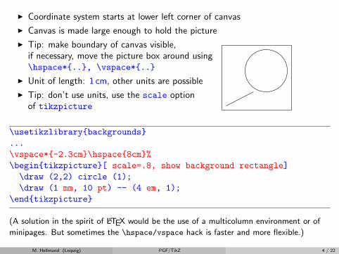
I Coordinate system starts at lower left corner of canvas

I Canvas is made large enough to hold the picture

I Tip: make boundary of canvas visible,if necessary, move the picture box around using\hspace*{..}, \vspace*{..}

I Unit of length: 1 cm, other units are possible

I Tip: don’t use units, use the scale optionof tikzpicture

\usetikzlibrary{backgrounds}...\vspace*{-2.3cm}\hspace{8cm}%\begin{tikzpicture}[ scale=.8, show background rectangle]\draw (2,2) circle (1);\draw (1 mm, 10 pt) -- (4 em, 1);

\end{tikzpicture}

(A solution in the spirit of LATEX would be the use of a multicolumn environment or of

minipages. But sometimes the \hspace/vspace hack is faster and more flexible.)


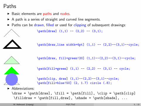
PathsI Basic elements are paths and nodes.

I A path is a series of straight and curved line segments.

I Paths can be drawn, filled or used for clipping of subsequent drawings:

\path[draw] (1,1) -- (2,2) -- (3,1);

\path[draw,line width=4pt] (1,1) -- (2,2)--(3,1)--cycle;

\path[draw, fill=green!20] (1,1)--(2,2)--(3,1)--cycle;

\path[fill=green] (1,1) -- (2,2) -- (3,1) -- cycle;

\path[clip, draw] (1,1)--(2,2)--(3,1)--cycle;

\path[fill=blue!50] (2, 1.7) circle (.8);

I Abbreviations:\draw = \path[draw], \fill = \path[fill], \clip = \path[clip]\filldraw = \path[fill,draw], \shade = \path[shade], ...


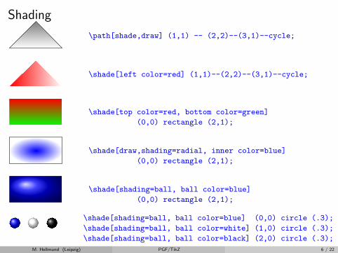
Shading

\path[shade,draw] (1,1) -- (2,2)--(3,1)--cycle;

\shade[left color=red] (1,1)--(2,2)--(3,1)--cycle;

\shade[top color=red, bottom color=green]

(0,0) rectangle (2,1);

\shade[draw,shading=radial, inner color=blue]


\shade[shading=ball, ball color=blue]


\shade[shading=ball, ball color=blue] (0,0) circle (.3);

\shade[shading=ball, ball color=white] (1,0) circle (.3);

\shade[shading=ball, ball color=black] (2,0) circle (.3);


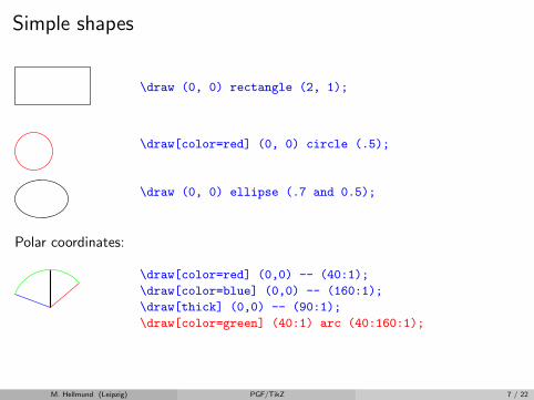
Simple shapes

\draw (0, 0) rectangle (2, 1);

\draw[color=red] (0, 0) circle (.5);

\draw (0, 0) ellipse (.7 and 0.5);

Polar coordinates:

\draw[color=red] (0,0) -- (40:1);

\draw[color=blue] (0,0) -- (160:1);

\draw[thick] (0,0) -- (90:1);

\draw[color=green] (40:1) arc (40:160:1);


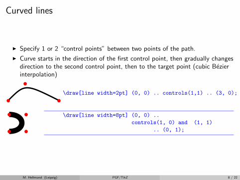
Curved lines

I Specify 1 or 2 “control points” between two points of the path.

I Curve starts in the direction of the first control point, then gradually changesdirection to the second control point, then to the target point (cubic Bezierinterpolation)

\draw[line width=2pt] (0, 0) .. controls(1,1) .. (3, 0);

\draw[line width=8pt] (0, 0) ..

controls(1, 0) and (1, 1)

.. (0, 1);


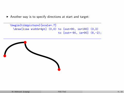
I Another way is to specify directions at start and target:

\begin{tikzpicture}[scale=.7]

\draw[line width=4pt] (0,0) to [out=90, in=180] (3,2)

to [out=-90, in=90] (8,-2);


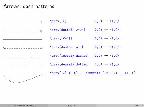
Arrows, dash patterns

\draw[->] (0,0) -- (1,0);

\draw[dotted, >->>] (0,0) -- (1,0);

\draw[|<->|] (0,0) -- (1,0);

\draw[dashed, o-)] (0,0) -- (1,0);

\draw[loosely dashed] (0,0) -- (1,0);

\draw[densely dotted] (0,0) -- (1,0);

\draw[->] (0,0) .. controls (.2,-.2) .. (1, 0);


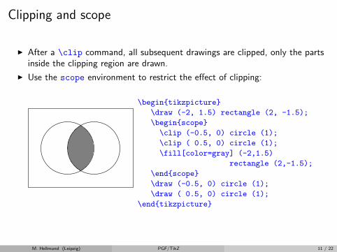
Clipping and scope

I After a \clip command, all subsequent drawings are clipped, only the partsinside the clipping region are drawn.

I Use the scope environment to restrict the effect of clipping:

\begin{tikzpicture}

\draw (-2, 1.5) rectangle (2, -1.5);

\begin{scope}

\clip (-0.5, 0) circle (1);

\clip ( 0.5, 0) circle (1);

\fill[color=gray] (-2,1.5)

rectangle (2,-1.5);

\end{scope}

\draw (-0.5, 0) circle (1);

\draw ( 0.5, 0) circle (1);

\end{tikzpicture}


Nodes

I Nodes are added to paths after the path is drawn:

A

B

\path[draw] (0, 0) node {A} -- (1,0) -- (1,1) node {B};

I Nodes can get a name for later references. Nodes have many options.

A2

B

\path[draw] (0, 0) node[draw] (nodeA) {$A^2$} -- (1,0)

-- (1,1) node[ellipse,fill=green](nodeB) {\tiny B};

\draw[red,->] (nodeA) -- (nodeB);

I It is often better to define named nodes first and connect them later, sincethen the paths are clipped around the notes. For this,

\path (x,y) node[Options] (node name) {TeX content of node}

can be written as

\node[Options] (node name) at (x,y) {TeX content of node}


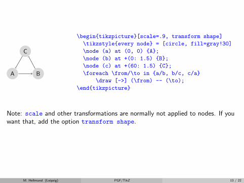
A B

C

\begin{tikzpicture}[scale=.9, transform shape]

\tikzstyle{every node} = [circle, fill=gray!30]

\node (a) at (0, 0) {A};

\node (b) at +(0: 1.5) {B};

\node (c) at +(60: 1.5) {C};

\foreach \from/\to in {a/b, b/c, c/a}

\draw [->] (\from) -- (\to);

\end{tikzpicture}

Note: scale and other transformations are normally not applied to nodes. If youwant that, add the option transform shape.


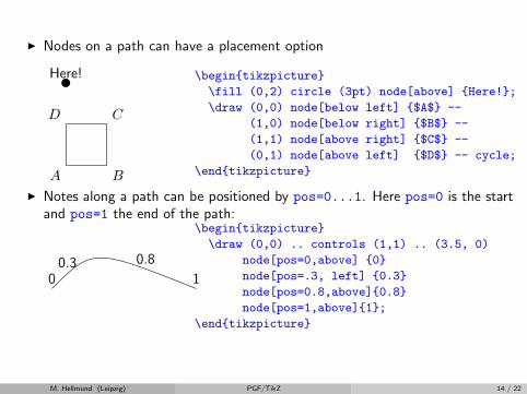
I Nodes on a path can have a placement option

Here!

A B

CD

\begin{tikzpicture}

\fill (0,2) circle (3pt) node[above] {Here!};

\draw (0,0) node[below left] {$A$} --

(1,0) node[below right] {$B$} --

(1,1) node[above right] {$C$} --

(0,1) node[above left] {$D$} -- cycle;

\end{tikzpicture}

I Notes along a path can be positioned by pos=0...1. Here pos=0 is the startand pos=1 the end of the path:

00.3 0.8

1

\begin{tikzpicture}

\draw (0,0) .. controls (1,1) .. (3.5, 0)

node[pos=0,above] {0}

node[pos=.3, left] {0.3}

node[pos=0.8,above]{0.8}

node[pos=1,above]{1};

\end{tikzpicture}


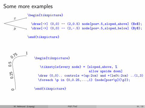
Some more examples

x

y

\begin{tikzpicture}

\draw[->] (0,0) -- (2,0.5) node[pos=.5,sloped,above] {$x$};

\draw[->] (0,0) -- (2,-.5) node[pos=.5,sloped,below] {$y$};

\end{tikzpicture}

00.

250.

5

0.75 1\begin{tikzpicture}

\tikzstyle{every node} = [sloped,above, %

allow upside down]

\draw (0,0).. controls +(up:2cm) and +(left:2cm) ..(1,3)

\foreach \p in {0,0.25,...,1} {node[pos=\p]{\p}};

\end{tikzpicture}


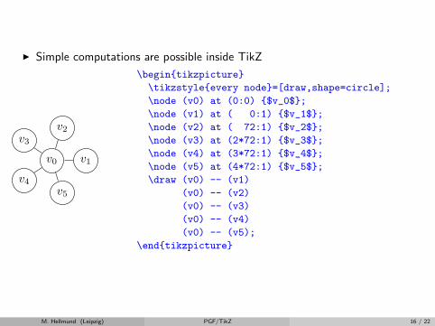
I Simple computations are possible inside TikZ

v0 v1

v2

v3

v4

v5

\begin{tikzpicture}

\tikzstyle{every node}=[draw,shape=circle];

\node (v0) at (0:0) {$v_0$};

\node (v1) at ( 0:1) {$v_1$};

\node (v2) at ( 72:1) {$v_2$};

\node (v3) at (2*72:1) {$v_3$};

\node (v4) at (3*72:1) {$v_4$};

\node (v5) at (4*72:1) {$v_5$};

\draw (v0) -- (v1)

(v0) -- (v2)

(v0) -- (v3)

(v0) -- (v4)

(v0) -- (v5);

\end{tikzpicture}


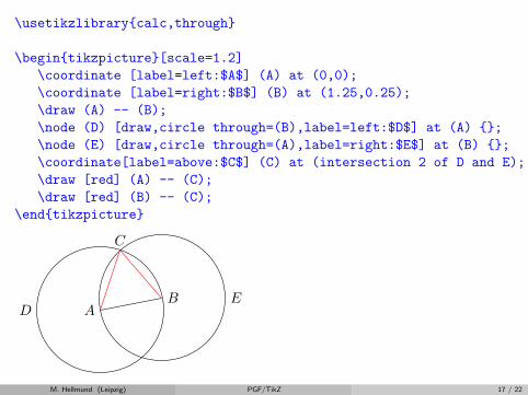
\usetikzlibrary{calc,through}

\begin{tikzpicture}[scale=1.2]\coordinate [label=left:$A$] (A) at (0,0);\coordinate [label=right:$B$] (B) at (1.25,0.25);\draw (A) -- (B);\node (D) [draw,circle through=(B),label=left:$D$] at (A) {};\node (E) [draw,circle through=(A),label=right:$E$] at (B) {};\coordinate[label=above:$C$] (C) at (intersection 2 of D and E);\draw [red] (A) -- (C);\draw [red] (B) -- (C);

\end{tikzpicture}

AB

DE

C


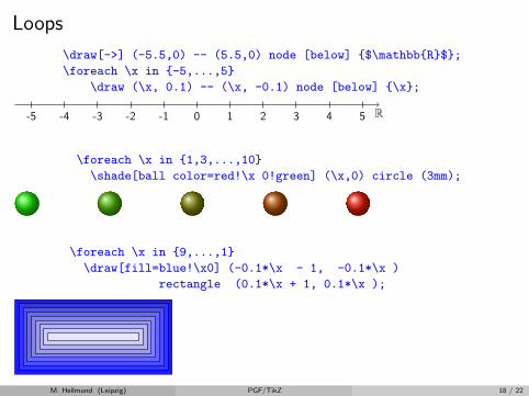
Loops

\draw[->] (-5.5,0) -- (5.5,0) node [below] {$\mathbb{R}$};

\foreach \x in {-5,...,5}

\draw (\x, 0.1) -- (\x, -0.1) node [below] {\x};

R-5 -4 -3 -2 -1 0 1 2 3 4 5

\foreach \x in {1,3,...,10}

\shade[ball color=red!\x 0!green] (\x,0) circle (3mm);

\foreach \x in {9,...,1}

\draw[fill=blue!\x0] (-0.1*\x - 1, -0.1*\x )

rectangle (0.1*\x + 1, 0.1*\x );


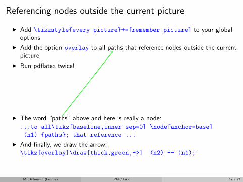
Referencing nodes outside the current picture

I Add \tikzstyle{every picture}+=[remember picture] to your globaloptions

I Add the option overlay to all paths that reference nodes outside the currentpicture

I Run pdflatex twice!

I The word “paths” above and here is really a node:...to all\tikz[baseline,inner sep=0] \node[anchor=base](n1) {paths}; that reference ...

I And finally, we draw the arrow:\tikz[overlay]\draw[thick,green,->] (n2) -- (n1);


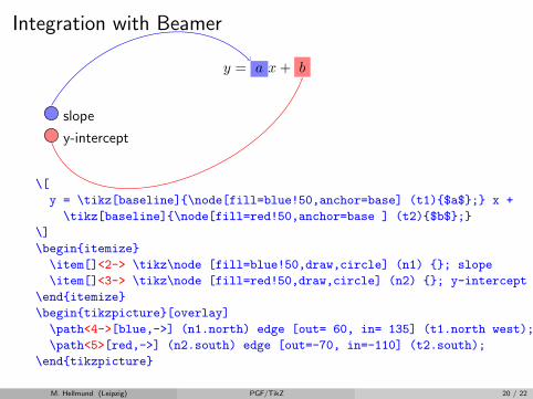
Integration with Beamer

y = a x + b

slope

y-intercept

\[

y = \tikz[baseline]{\node[fill=blue!50,anchor=base] (t1){$a$};} x +

\tikz[baseline]{\node[fill=red!50,anchor=base ] (t2){$b$};}

\]

\begin{itemize}

\item[]<2-> \tikz\node [fill=blue!50,draw,circle] (n1) {}; slope

\item[]<3-> \tikz\node [fill=red!50,draw,circle] (n2) {}; y-intercept

\end{itemize}

\begin{tikzpicture}[overlay]

\path<4->[blue,->] (n1.north) edge [out= 60, in= 135] (t1.north west);

\path<5>[red,->] (n2.south) edge [out=-70, in=-110] (t2.south);

\end{tikzpicture}


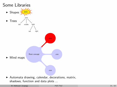
Some Libraries

I Shapes BANG!

I Treesroot

left middle right

left right

I Mind mapsRoot concept

child

child

child

I Automata drawing, calendar, decorations, matrix,shadows, function and data plots ...


References

I A great source of examples, tutorials etc ishttp://www.texample.net/tikz/

I Some examples were taken fromhttp://altermundus.fr/pages/downloads/remember beamer.pdf,http://www.statistiker-wg.de/pgf/tutorials.htmandhttp://www.tug.org/pracjourn/2007-1/mertz/

I and of course from the PGF/TikZ Manual.


a tutorial meik hellmund - uni-leipzig.dehellmund/latex/pgf-tut.pdf · pgf and tikz i according to...

Documents