A Two-Element DirectionalAntenna for Coupling Wireless

Signals into HVAC Ducts

Jessica Hess

2005

Advisor: Prof. Star~ci|

Carnegie Mellon University

A Two-Element Directional Antenna for Coupling

Wireless Signals into HVAC Ducts

A Thesis

Submitted to the Department of Electrical and Computer Engineering

In Partial Fulfillment of the Requirements

For the

Master of Science

in

Electrical and Computer Engineering

By

Jessica C. Hess

Pittsburgh, PA 15213

August 5, 2005

Table of Contents

Table of Figures

List of Tables

Chapter 1: Introduction

1.1 Project Description

1.2 Report Overview

Chapter 2: Iterative Design of the Antenna

2.1 Monopole

2.2. Reflector

2.3 Ducts and T-junction

2.4 Experimental Setup

2.5 First Distance Iteration

2.6 Length Iteration

2.7 Second Distance Iteration

Chapter 3: Data Analysis and Results

3.1 Data Analysis

3.2 Results

Chapter 4: Analysis of the Design

4.1 Analysis

4.2 Tests

4.3 Conclusion

Works Cited

Appendix A: MATLAB Code

Table of Ficlures

Figure

Figure

Figure

Figure

Figure

Figure

Figure

Figure

Figure

Figure

Figure

Figure

Figure

Figure

Figure

Figure

1 : Signal strengths for wireless-in-HVAC system, monopole antenna.

2: Signal strengths for wireless-in-HVAC system, untuned directional antenna.

3: Configuration of the prototype antenna.

4: Plot of correlation between signal strength and throughput.

5: Monopole antenna.

6: Reflector.

7: Hole in HVAC duct with metal neck.

8: Mode filtering by T-junction.

9: Experimental setup.

10: First distance iteration results.

11: Length iteration results.

12: Second distance iteration results.

13: Configuration of elements for the antenna design.

14: Return loss, for monopole and directional antenna cases.

15: Three strongest modes, normalized to the theoretical value of TE61.

16: Three strongest modes, normalized to theoretical and extracted TE61 value.

List of Tables

Table 1 : Dimensions of optimized antenna design.

Table 2: Average performance of optimized directional antennaover the frequency range 2.4-2.4835GHz.

Chapter 1: Introduction

One of a modern business’ most valuable assets is its communications

infrastructure: without it, there is no connection to the outside world, no way to interface

with customers, and no way to move data to where it needs to go. As the need for fast

and convenient communication increases, the cost of wiring buildings and providing

mobility for individual employees is also increasing. Over time, more businesses are

employing high-speed wireless technology, either in addition to their wired

infrastructures or in place of them; however, attempting to use conventional wireless

products and methodologies to meet all communication needs can be problematic. First,

as access points (APs) tend to be centrally located, often in hallways, their signal tends

to illuminate corridors and other unpopulated areas better than the most important areas,

offices and conference rooms. Also, areas further from the access point tend to get

significantly lower signal quality and data rates.

A promising method for addressing the problem described above involves

installing wireless networking equipment in heating, ventilation, and air conditioning

(HVAC) ducts and using them as waveguides. The nature of ventilation ducts is such

that the signal they deliver will be strongest in areas where employees spend most of

their time--offices and conference rooms--because this is where vents open, both

ventilating the room and allowing transference of wireless signals. A group of students

within the Antenna and Radio Communications Group have been working on wireless-in-

duct technology for several years, sponsored by ABB, YIT, and the National Science

Foundation [1]-[17]. This project is a continuation of these efforts.

For much of the other research done on implementation of wireless networking

within HVAC ducts, an AP is pigtailed to an external monopole, which is then placed into

the duct. However, in many HVAC systems, the use of a directional antenna rather than

a simple monopole would improve performance significantly: a monopole placed in a

duct transmits more or less bidirectionally, which can be unnecessary, as in the case

when only one section of a building needs to be illuminated, and signal transmitted in the

other direction is "wasted." Bidirectional transmission can even, in many cases, increase

dispersion of the signal, which decreases throughput. For instance, the most convenient

placement of an antenna may be near air-handling equipment, tapers, end caps, or other

features of the duct which could disrupt the signal. A reflection from one of these

features will be offset in time and phase from the signal that was originally transmitted,

making reception and decoding of the original signal more difficult. If, however, a

directional antenna is used, then not only will there be an increase in the amplitude of

the original signal, but the amplitude of the reflected signal will decrease, perhaps

enough so that the reflected signal can be ignored by the receiver.

1.1 Project Description

For this project, I designed a two-element directional antenna for use in

networking via IEEE 802.1 lb/g within heating, ventilation, and air conditioning (HVAC)

ducts. My goal was to maximize for the best average forward gain, given a pre-chosen

driven element and a single other element acting as a reflector. In order to maximize

forward gain, I varied the length of the second element, as well as the distance between

it and the driven element. The test setup was designed carefully, so that the

configuration I determined to be optimal would work well in a general HVAC duct

environment.

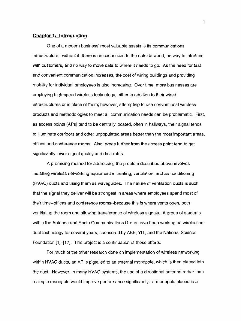
Figures 1 and 2 show the results of a series of signal power measurements taken

by Ben Henty from a wireless-in-duct installation, first with a simple monopole, then with

an early prototype of a two-element directional antenna, which had not been optimized.

The prototype, a diagram of which is shown in Figure 3, consisted of the monopole, with

a reflector made of 1/16" diameter welding rod placed several inches away from, but in

line with it. Even without proper tuning of the length or inter-element distance of the

directional antenna, there is noticeable change in signal strength throughout much of the

building. The directional antenna gives an average gain of 1 .ldB in the forward direction

and a loss of 0.8dB in the reverse direction. A properly designed directional antenna

would have better gain and therefore more striking results.

10

9

8

7

6

5

4

3

2

1

0

6 7 8 10 11 12 13

Figure 1 : Signal strengths for wireless-in-duct system, monopole antenna [17].

4

10

9

/ of maxi i .v ..................: ................:.-antenna. ..........

l i radiation ::

6 7 8 9 10 11 12 13

Figure 2: Signal strengths for wireless-in-duct system, untuned directional antenna [17].

length

reflector

inter-elementdistance

rnonopole

Figure 3: Configuration of the prototype antenna.

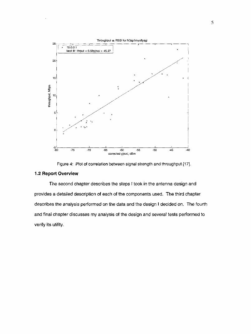
There was a strong correlation between the received signal strength and the

throughput for IEEE 802.1 lg in this experiment, as shown in Figure 4. Given the strong

correlation between signal strength and throughput, in addition to rather promising

results for an untuned directional antenna, further optimization of the directional antenna

design seemed justified.

25

15

Throughput vs RSSI for flr3aplmyoffyagi

10.0.0.1best fit: thrput = O.59yjrssi + 45.27

x

-5 L~~ I r ~ I-80 -75 -70 -65 -60 -55 -50 -45 -40

corrected yjrssi, dBm

Figure 4: Plot of correlation between signal strength and throughput [17].

1.2 Report Overview

The second chapter describes the steps I took in the antenna design and

provides a detailed description of each of the components used. The third chapter

describes the analysis performed on the data and the design I decided on. The fourth

and final chapter discusses my analysis of the design and several tests performed to

verify its utility.

Chapter 2: Iterative Desiqn of the Antenna

This chapter describes the set of experiments performed in the process of

designing this antenna, as well as the materials used. Certain aspects of the

experimental setup are worth examining; explanations of the thought process leading to

these decisions are provided.

The goal was to create a two-element directional antenna, inspired by the Yagi-

Uda design [18] and [19], which would improve the strength and quality of an IEEE

802.1 lb/g signal being transmitted through an HVAC. duct system. The design

progressed as a series of "experiments," iteratively determining the best combination of

distance between elements and reflector length. The first experiment consisted of

variation over inter-element distance; the second consisted of variation over length; and

the third consisted of variation over distance again. Before the experimental setup can

be described in detail, a full description of the components is in order.

2.1 Monopole

The monopoles, illustrated in Figure 5, are constructed from SMA female right-

angle panel mount connectors with extended dielectric, screwed to brass bases with

holes through the center. Metallic "teeth," inter~ded to snap the fixture into a ten

millimeter hole in the side of a duct, have been placed into the base, around the

dielectric. The dielectric has been cut down to be level with the brass base, leaving the

center conductor exposed. A brass cylinder with a hole in it has been fitted onto the end

of the center conductor.

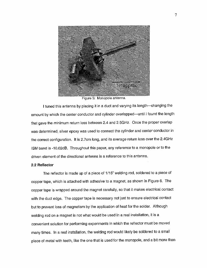
Figure 5: Monopole antenna.

I tuned this antenna by placing it in a duct and varying its length--changing the

amount by which the center conductor and cylinder overlapped--until I found the length

that gave the minimum return loss between 2.4 and 2.5GHz. Once the proper overlap

was determined, silver epoxy was used to connect the cylinder and center conductor in

the correct configuration. It is 2.7cm long, and its average return loss over the 2.4GHz

ISM band is -10.02dB. Throughout this paper, any reference to a monopole or to the

driven element of the directional antenna is a reference to this antenna.

2.2 Reflector

The reflector is made up of a piece of 1/16" welding rod, soldered to a piece of

copper tape, which is attached with adhesive to a magnet, as shown in Figure 6. The

copper tape is wrapped around the magnet carefully, so that it makes electrical contact

with the duct edge. The copper tape is necessary not just to ensure electrical contact

but to prevent loss of magnetism by the application of heat for the solder. Although

welding rod on a magnet is not what would be used in a real installation, it is a

convenient solution for performing experiments in which the reflector must be moved

many times. In a real installation, the welding rod would likely be soldered to a small

piece of metal with teeth, like the one that is used for the monopole, and a bit more than

a millimeter should be added to its length, to account for the absence of the magnet.

Figure 6: Reflector.

The distance between the reflector and the driven element is measured by

means of a plastic ruler taped into the duct. The magnet is of sufficient strength that it

stays firmly attached to the side of the duct, but it is not difficult to remove it between

measurements.

2.3 Ducts and T-Junction

I used one foot diameter by ten foot long cylindrical galvanized steel HVAC ducts,

connected end to end, for these experiments. One section had a 190mm hole cut out of

its side at ninety degrees off the antennas’ axis, with a metal neck attached, like that

shown in Figure 7. The purpose of the hole was to change the propagation environment

in order to make the resulting antenna design more useful for a real-world system, where

features such as T-junctions and bends are common.

Figure 7: Hole in HVAC duct with metal neck.

The authors of [13] found that the power level of a signal excited by a monopole

was decreased by approximately 9dB after passing a single T-junction. Every T-junction

after the first resulted in a 3dB decrease in signal strength, which is the expected

response of a power splitter. The hypothesis, which [14] and [15] found to be correct,

was that mode filtering occurred at the first T-junction. The dominant mode excited by a

quarter-wave monopole is TE61, which propagates rather slowly and is greatly

attenuated by large holes, as shown in Figure 8. The impulse response shows the

separate arrival of the TE61 and TE~I modes. TE6~ has the largest amplitude in the

absence of a hole, while TEs~ has the largest amplitude after passing by a 190mm

diameter hole.

Figure 8: Mode filtering by T-junction. [1 4]

Had these experiments been done with a straight section of duct, without a hole,

they would likely have ended in an antenna design that maximized TE61. This would

have been of little use in practice, as most duct systems have many branches, and

maximization of TE61 would not lead to much gain, in general, as it would be filtered out

upon passing T-junctions.

2.4 Experimental Setup

The experiment was set up as shown in Figure 9, with four ducts connected end

to end and a hole placed in the third, to mimic a T-junction. The antenna under test was

used as the transmitter, and a monopole was used as the receiver. Measurements were

done with an HP 8714B vector network analyzer (VNA). A fifty foot coaxial cable

connected the VNA to the transmitting antenna, and a six foot SMA cable went to the

receiver. Both cables were calibrated out before any measurements were taken.

I

Figure 9: Experimental setup.

If data were to be taken only at one receiver position, we would end with an

antenna design that was optimal for that specific placement but which would not

necessarily work well in general. Because the goal was to design an antenna that would

work well in most cases, rather than one that works for one specific case, I made ten

holes for the receiving antenna, each approximately 12cm apart, and measured the

received signal at each one for every scenario under test. I then averaged my results

from these ten receiver positions, to get one "average" result for each test scenario. The

choice of 12cm as the distance between receiver positions was because it has been

found, experimentally, that in order to have a correlation of below 0.4, antennas in ducts

of the dimensions used in this experiment must be at least 12cm apart [16]. Taking the

average would only be truly valuable if the measurements were minimally correlated.

The first step, before I could begin the iteration of element distance or length,

was to measure the channel using a monopole without a reflector for transmission. This

measurement served as my "base" case, from which I could determine how much gain a

particular reflector configuration had achieved. I took this measurement at each of the

ten receiver positions and averaged, just as I did for each of the test cases.

2.5 First Distance Iteration

The first experiment involved varying the distance between the driven element

and the reflector. For this iteration, I chose to make the reflector 5.5cm long,

approximately twice the length of the driven element. This length stayed constant

throughout the experiment. I found that the closest I could reasonably get the reflector

to the driven elemen~t was 2.5cm, so this was my starting point. From there, I increased

the distance by 0.Scm each time, ending at 12cm. Using the methods described in

Chapter Three, I found that the distance that provided the highest gain was 3cm.

2.6 Length Iteration

For the second experiment, I placed the reflector ~hree centimeters from the

driven element. The distance stayed constant throughout this iteration. Because I was

using wire cutters on welding rod, I found that the best granularity available for element

length was about a quarter centimeter. Therefore, I measured the channel, starting at a

length of 5.25cm, decreasing by 0.25cm for each measurement, and ending at 2.5cm,

which was slightly less than the length of the driven element. The length that provided

the highest gain at a distance of 3cm was 3cm. It should be noted that the margin of

error was greater th;an the height of the magnet.

2.7 Second Distance Iteration

I performed the final iteration much like the first, using a fixed-length reflector of

3cm, rather than 5.5cm. The starting distance between elements was 2.5cm; again, I

increased the distance by half a centimeter for each measurement and ended at 12cm.

The distance that provided the highest gain with this final iteration was 5cm.

Chapter 3: Data Analysis and Results

This chapter describes the steps involved in analyzing the data from each

iteration of the design and provides a description of the results.

3.1 Data Analysis

Each combination of distance, length, and receiver position yielded a file with

1601 magnitudes equally spaced across 100MHz, from 2.4 to 2.5GHz. The first step

was to read in the data and cut it down to only represent the IEEE 802.11 b/g spectrum,

2.4 to 2.4835GHzu Next, the data had to be averaged across receiver positions to

provide one "general" set of data per test scenario; in order to properly reflect received

signal power, the average was done on the linear magnitudes, rather than in logarithmic

scale. Once the data from all the receiver positions were averaged together, the

analysis broke into two separate paths: one ended in finding an average gain across the

entire spectrum, and the other weighted the spectrum differently, finding the average

IEEE 802.11 channel gain, instead.

In order to find the average gain across the spectrum, I averaged across

frequency, again in linear scale, to get one number for received power per test scenario.

This number was converted back to logarithmic scale, and the average for the

monopole-only case,, computed in the same manner, was subtracted from it to give a

value for gain. For the remainder of the chapter, this number will be referred to as the

"average full-spectrum gain" for the reflector configuration under discussion.

In order to weight the data to better represent the gain one would expect to find in

IEEE 802.11 channels, I took the data points that corresponded to each channel in turn

and averaged those,, in linear scale, across frequency. Because of the overlap in IEEE

802.11 channels, many points were averaged several times, into several different

numbers. I averaged over each of the thirteen channels separately, in linear scale, for

both the monopole-only case and each of the test cases, and then I subtracted to find

the gain per channel. Because the value I wanted to find was the expected value of

what one would measure in channel gain, and because these measurements tend to be

done in decibel values, the last average, across the thirteen channels, was done in

logarithmic scale. Tl~is number will be referred to as "average channel gain."

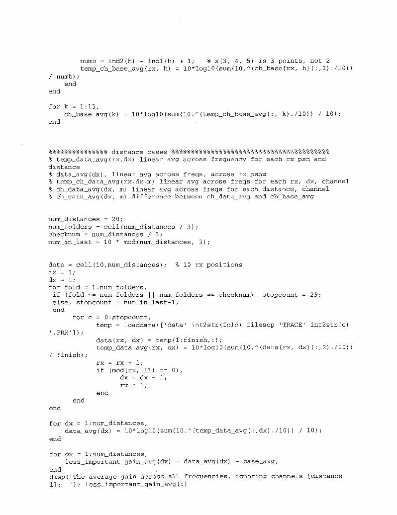
The MATLAB code is included in Appendix Ao

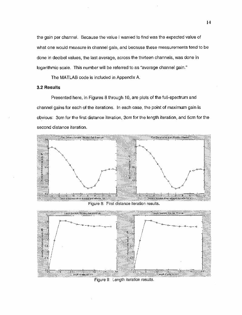
3.2 Results

Presented here, in Figures 8 through 10, are plots of the full-spectrum and

channel gains for each of the iterations. In each case, the point of maximum gain is

obvious: 3cm for the first distance iteration, 3cm for the length iteration, and 5cm for the

second distance iteration.

Figure 8: First distance iteration results.

Figure 9: Length iteration results.

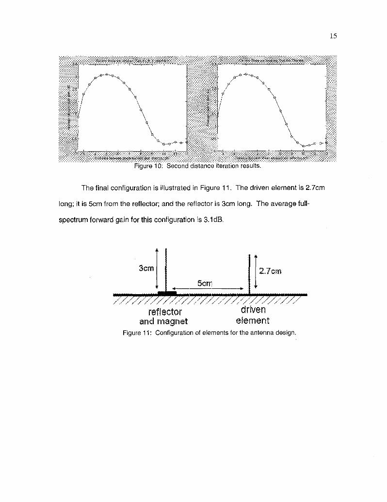
Figure 10: Second distance iteration results.

The final configuration is illustrated in Figure 11. The driven element is 2.7cm

long; it is 5cm from the reflector; and the reflector is 3cm long. The average full-

spectrum forward gain for this configuration is 3.1dBo

5cr~

2.7cm

reflector drivenand magnet element

Figure 11 : Configuration of elements for the antenna design.

Chapter 4: Analysis of the Desiqn

This chapter discusses the antenna design in light of current understanding about

directional antennas and propagation in tt~e HVAC duct environment. 1 performed two

simple tests to confirm that the design was reasonable, and those results are also

presented.

4.1 Analysis

The generally accepted distance between the first reflector and the driven

element in an antenna based off the Yagi-Uda design is one quarter wavelength, which

gives a 90 degree phase shift of the signal propagating to the reflector, a 180 degree

phase shift from the reflection itself, and another 90 degree phase shift in propagating

back to the starting point, making the reflected signal in phase with the signal emitted by

the driven element. The reflector itself should be a little bit, but not much, longer than

the driven element; the general rule of thumb is five percent longer. The added length

changes the mutual impedance and thereby the relative current phases in the two

elements so that constructive interference occurs in the forward direction.

Under the assumption that this antenna works in the same way as the Yagi-Uda

antenna [18] and [19], finding an optimum reflector length of 3cm is encouraging: 3cm is

the length increment closest to but definitively longer than the driven element’s length.

The increment referred to as "2.75" could, given the margin of error involved in using

wire cutters on welding rod, end up shorter than the driven element. The theoretically

optimum length, using the ffive percent longer" rule, is 2.84cm.

Again, assurning that this antenna design is in agreement with the Yagi-Uda

antenna design, the spacing of 5cm reflects a wavelength of 20cm. This is in close

agreement with the wavelength of mode TE51, 20.6cm, as shown in [15]. As TE51 is the

mode with the second largest magnitude excited by a monopole in a cylindrical duct, and

as shown in Figure 8, the presence of a "[-junction does not reduce its magnitude by

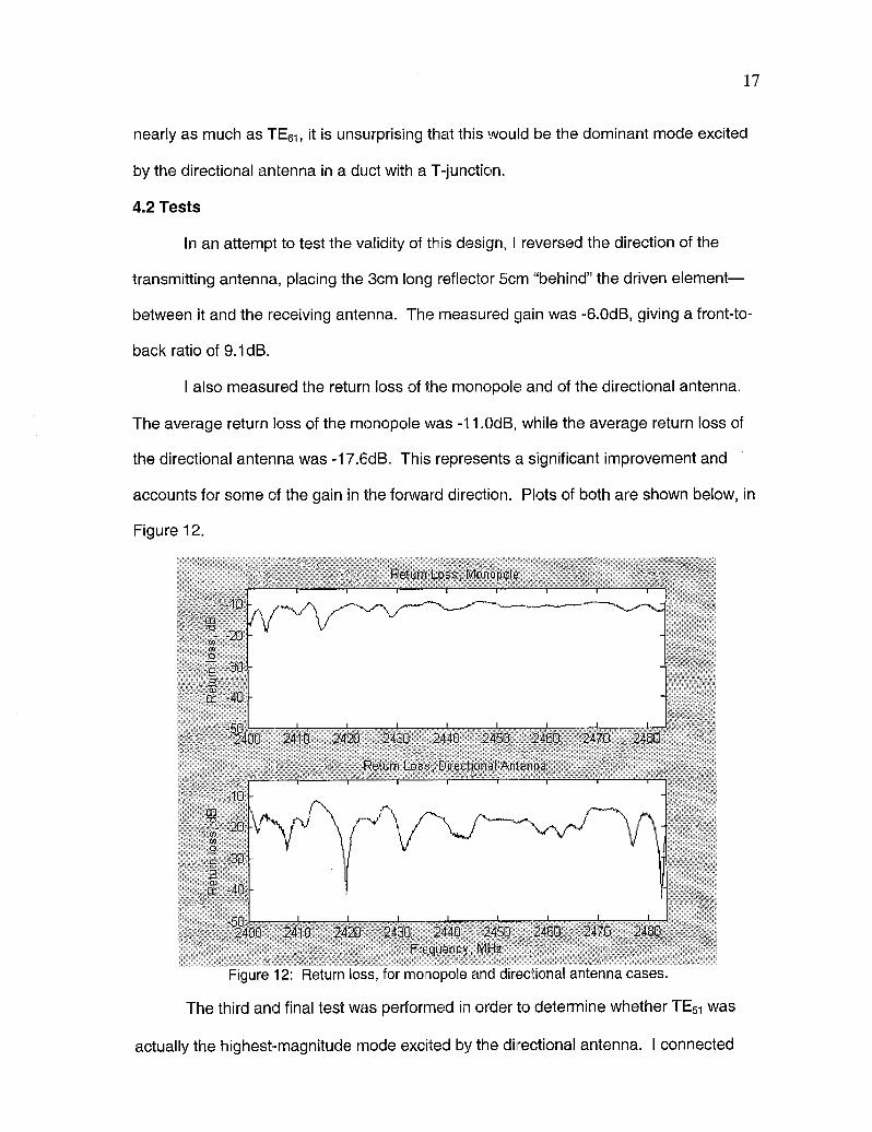
nearly as much as TE61, it is unsurprising that this would be the dominant mode excited

by the directional antenna in a duct with a T-junction.

4.2 Tests

In an attempt to test the validity of this design, I reversed the direction of the

transmitting antenna, placing the 3cm long reflector 5cm "behind" the driven element--

between it and the receiving antenna. The measured gain was -6.0dB, giving a front-to-

back ratio of 9.1dB.

I also measured the return loss of the monopole and of the directional antenna.

The average return loss of the monopole was -1 1.0d8, while the average return loss of

the directional antenna was -17.6dB. This represents a significant improvement and

accounts for some of the gain in the forward direction. Plots of both are shown below, in

Figure 12.

Figure 12: Return loss, for monopole and directional antenna cases.

The third and final test was performed in order to determine whether TE51 was

actually the highest.-magnitude mode excited by the directional antenna. I connected

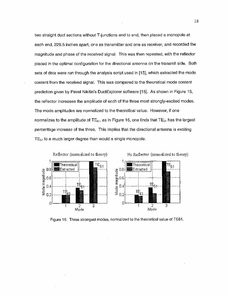
18

two straight duct sections without T-junctions end to end, then placed a monopole at

each end, 229.5 inches apart, one as transmitter and one as receiver, and recorded the

magnitude and phase of the received signal. This was then repeated, with the reflector

placed in the optimal configuration for the directional antenna on the transmit side. Both

sets of data were run through the analysis script used in [15], which extracted the mode

content from the received signal. This was compared to the theoretical mode content

prediction given by Pavel Nikitin’s DuctExplorer software 1115]. As shown in Figure 15,

the reflector increases the amplitude of each of the three most strongly-excited modes.

The mode amplitudes are normalized to the theoretical value. However, if one

normalizes to the amplitude of TEe1, as in Figure 16, one finds that TEsl has the largest

percentage increase of the three. This implies that the directional antenna is exciting

TEs~ to a much larger degree than would a single monopole.

No l~.e~]ector (~orm~lized to ~eory)

I I

0.8

0.6

~.2

ITheoretical ; TE~Ext act~

61

...... ....1 2

Mode

0 01 2 3

Mode

1

Figure 15: Three strongest modes, normalized to the theoretical value of TE61.

19

Reflector (normalized to TE61) 14o Reflector (nmrnalized to TE61)

1

0 01 2 3 1 2 3

Mode Mode

Figure 16: Three strongest modes, normalized to theoretical and extracted TE61 value.

4.3 Conclusion

The final parameters and performance of the optirnized antenna are summarized

in Tables 1 and 2, respectively.

The design of this directional antenna, produced by iteration over length and

inter-element distance with maximization for forward gain, makes sense from a

theoretical standpoint. An inter-element distance of 5cm is consistent with previous

findings about mode content in ducts with T-junctions, and the reflector length of 3cm is

consistent with Yagi-Uda’s antenna design. It also has a low VSWR and a high front-to-

back ratio. These attributes make the antenna an attractive component for improving

the performance of wireless-in-duct systems. The high front-to-back ratio helps to

reduce unwanted reflections and reduce interference, while the gain of the antenna

enables better signal strength in areas to be covered. Referring to Figure 4, a signal

level increase of 3.1dB should lead to an average expected increase in throughput of

about 1.8Mbps. Consequently, the antenna designed for this project and described in

this paper should be; valuable for future wireless-in-duct installations.

2O

Driven element lengthDriven element diameter

Reflector lengthReflector diameter

2.7cm0.3175cm (1/8 in.)

3cm0.1588cm (1/16 in.)

Element spacing 5cmTable 1: Dimensions of optimized antenna design.

Gain 3.1dBFront-to-back ratio 9.1 dB

Return loss -17.6dB-I"able 2: Average performance of optimized directional

antenna over the frequency range 2.4-2.4835GHz.

Works Cited

[i]

[2]

[3]

[4]

[6]

[7]

[8]

[9]

[lO]

[11]

D.D. Stancil, O.K. Tonguz, A. Xhafa, A. Cepni, P. Nikitin, and D. Brodtkorb, "High-speedInternet access via HVAC ducts: a new approach," IEEE Global TelecommunicationsConference, 2001, pt. 6, p 3604-7 volo6.

A.E. Xhafa, O.Z. Tonguz, A.G. Cepni, D.D. Stancil, P.V. Nikitin, and D. Brodtkorb,"Theoretical estimates of HVAC duct channel capacity for high-speed Internet access,"IEEE International Conference on Communications, 2002, pt. 2, p 936-9 vol.2.

P.V. Nikitin, D.D. Stancil, O.K. Tonguz, A.E. Xhafa, A.G. Cepni, and D. Brodtkorb, "RFpropagation in an HVAC duct system: impulse response characteristics of the channel,"IEEE Antennas and Propagation Society International Symposium, 2002, pt. 1, p 726-9vol.1.

A.G. Cepni, A.E. Xhafa, P.V. Nikitin, D.D. Stancil, O.K. Tonguz, "Multi-carrier signaltransmission through HVAC ducts: experimental results for channel capacity,"IEEE 56th Vehicular Technology Conference, 2002, pt. 1, p 331-5 vol.1.

[5] P.V. Nikitin, D.D. Stancil, A.G. Cepni, O.K. Tonguz, A.E. Xhafa, and D.Brodtkorb, "Propagation model for the HVAC duct as a communication channel," IEEETransactions on Antennas and Propagation, v 51, n 5, May 2003, p 945-51.

P.V. Nikitin, DoD. Stancil, A.G. Cepni, A.E. Xhafa, C).K. Tonguz, D. Brodtkorb,"Propagation modeling of complex HVAC networks using transfer matrix method [indoorcommunication application]," IEEE Antennas and Propagation Society InternationalSymposium, 2003, pt. 2, p 126-9 vol.2

A.E. Xhafa, P. Sonthikorn, O.K. Tonguz, P.V. Nikitin, A.G. Cepni, D.D. Stancil, B. Henty,and D. Brodtkorb, "Seamless handover in buildings using HVAC ducts: a new systemarchitecture," IEEE Global Telecommunications Conference, 2003, pt. 6, p 3093-7 vol.6.

P.V. Nikitin, D.D. Stancil, O.K. Tonguz, A.E. Xhafa, A.G. Cepni, and D. Brodtkorb,"Impulse response of the HVAC duct as a communication channel," IEEE Transactionson Communications, v 51, n 10, Oct. 2003, p 1736-42.

P.V. Nikitin, D.D. Stancil, A.G. Cepni, A.E. Xhafa, O.K. Tonguz, and D. Brodtkorb, "Anovel mode content analysis technique for antennas in multimode waveguides," IEEETransactions on Microwave Theory and Techniques, v 51, n 12, Dec. 2003, p 2402-8.

A. G. Cepni, D.D. Stancil, and D. Brodtkorbt, "Experimental mode content analysistechnique for complex overmoded waveguide systerns," IEEE Antennas andPropagation Society Symposium, 2004, pt. 3, p 2991-4 Vol.3

O.K. Tonguz, A.E. Xhafa, D.D. Stancil, A.G. Cepni, P.V. Nikitin, and D. Brodtkorb, "Asimple path-loss prediction model for HVAC systems," IEEE Transactions on VehicularTechnology, v 53, n 4, July 2004, p 1203-14.

[12] A.E. Xhafa, O.K. Tonguz, A.G. Cepni, D.D. Stancil, PoV. Nikitin, D. Brodtkorb, "On thecapacity limits of HVAC duct channel for high-speed Internet access," IEEE Transactionson Communications, v 53, n 2, Feb. 2005, p 335-42.

[13] O. K. Tonguz, D. D. Stancil, A. E. Xhafa, A. G. Cepni, P. V. Nikitin, and D. Brodtkorb,"An empirical path loss model for HVAC duct channel," IEEE Global CommunicationsConference, vol. 2, pp. 1850-1854, Taipei, Taiwan, 2002.

[14] Benjamin E. Henty and Daniel D. Stancil, "Improved Wireless Performance from ModeScattering in Ventilation Ducts," Antennas and Propagation Society Symposium, 2005.

[15] Nikitin, Pavel V. "Analysis of Heating, Ventilation, and Air Conditioning Ducts as a RadioFrequency Communication Channel." Ph.D. Dissertation, Carnegie Mellon UniversityElectrical Engineering Department, Au~gust, 2002.

[16] A.G. Cepni, D.D.. Stancil, A.E. Xhafa, Bo Henty, P.V. Nikitin, O.K. Tonguz, and D.Brodtkorb, "Capacity of multi-antenna array systems for HVAC ducts," IEEE InternationalConference on Communications, vol. 5, pp. 2934-2938, Paris, 2004.

[17]

[18]

B.E. Henty, unpublished.

C.A. Balanis, Antenna Theory, 3rd Edition, Wiley, 2005, p. 577, ff.

[19] H. Yagi, "Beam Transmission of Ultra Short Waves," Proceedings of the IRE, vol. 16, no.6, pp. 715-741, June 1928.

Appendix A: Matlab code

% break into channels, average the channels in dB. find average of% monopole (linear) and average of yagi (linear); subtract (in dB)

% average gain

clear;%%%%%%%%%%%%%%%%%% frequency vector %%%%%%%%%%%%%%%%%%%%%%%%%%%%%freq = zeros(1601,1);

foo = loaddata([’datal’ filesep ’TRACE0.PRN’]);freq : foo(:,l);

%%%%%%%%%%%%%%%%%% distances and lengths %%%%%%%%%%%%%%%%%%%%%%%%

dxs = 2.5:.5:12;lengths = 5.25:-.25::2.5;

%%%%%%%%%%%%%%%%% set up the thirteen channels %%%%%%%%%%%%%%%%%

channels : cell(l, 13);

center : 2412;for n = 1:13;

first = (center - 11.5);last = (center + 11.5);tmp : find((freq >= first) & (freq <: last));

indl(n) = tmp(1); % index of where channel begins in freqind2(n) = tmp(end); % index of where channel ends in freqchannels{n} = freq(indl:ind2);

center = center + 5;end

%%%%%%%%%%%%%%%% monopole case %%%%%%%%%%%%%%%%%%%%%%%%%%%%%%%%%%%%

% base_avg gets the average (linear) across all freqs, across the rx psns% temp_base_avg(rx_psn) gets the linear average across all freqs

% ch_base_avg(channel) gets the channel’s linear average across the rx psns

% loaddata puts the data into a 1601 x 2 matrix, magnitude & frequency

rx : i;

base = cell(10,1);for f : 0:9, % rx positions - zero to 9 is TEN!

temp = loaddata([’base’ filesep ’TRACE’ int2str(f) ’.PRN’]);toobig = find(temp(:,l) > 2483.5); % assumes all files the same...

assumption, though

finish = toobig(1) - % number of points

base{rx} = temp(l:finish,:);

temp_base_avg(rx) = lO*loglO(sum(lO.^(base{rx}(:,2)./lO) / finish);

rx : rx + i;endbase_avg = 10*logl0(sum(10.^(temp_base_avg./10)) /

freq = freq(l:finish);

OK

ch_base = cell(10,13);for rx = I:i0,

for h = 1:13,ch_base{rx, h] : base{rx}(indl(h) :ind2(h),:);

/ numb);end

end

numb = ind2(h) - indl(h) + i; % x(3, 4, 5) is 3 points,

temp. ch base_avg(rx, h) : 10*logl0(sum(10.^(ch_base{rx, h}(:,2)./10))

for k = 1:13ch_base_avg(k) = 10*logl0(sum(10.^(temp_ch_base_avg(:, k)./10))

end

%%%%%%%%%%%%%%% distance cases %%%%%%%%%%%%%%%%%%%%%%%%%%%%%%%%%%%%%%%%% temp_data_avg(rx,dx) linear avg across frequency for each rx psn and

distance% data_avg(dx), linear avg across freqs, across rx psns% temp. ch data_avg(rx, dx,m) linear avg across freqs for each rx, dx, channel

% ch_data_avg(dx, m) linear avg across freqs for each distance, channel% ch_gain_avg(dx, m) difference between ch_data_avg and ch_base_avg

num_distances = 20;

num_folders = ceil(num_distances / 3);checknum = num_distances / 3;

num in last = i0 * mod(num_distances, 3);

data = cell(10,num_distances);rx : i;

dx : i;for fold = l:num_folders,

% i0 rx positions

if (fold -= hum_folders I I num_folders == checknum), stopcount = 29;

else, stopcount =num in last-l;

endfor c = 0:stopcount,

temp = loaddata([’data’ int2str(fold) filesep ’TRACE’ int2str(c)

.PRN’]);data{rx, dx} = temp(l:finish,:);temp_data_avg(rx, dx) : 10*logl0(sum(10.^(data{rx dx}(:,2)

finish);

end

end

rx : rx + i;

if (mod(rx, ii) == dx : dx + i;rx : i;

end

for dx = l:num_distances,data_avg(dx) = 10*logl0(sum(10.^(temp_data_avg(:,dx)./10)

end

/ i0);

for dx = l:num_distances,less_important_gain_avg(dx) = data_avg(dx) - base_avg;

enddisp(’The average gain across all frequencies, ignoring channels [distance

i]: ’); less_important_gain_avg(:)

ch_data = cell(10,num_distances,13); % PAIN

for dx = l:num_distances,for rx = i:i0,

for m = 1:13,ch_data{rx, dx, m} : data{rx,dx}(indl(m):ind2(m),:);numb = ind2(m) - indl(m)

temp ch data_avg(rx,dx,m) = 10*logl0(sum(10.^(ch_data{rx, m}(:,2)./10)) / numb);

end

endend

for dx : l:num_distances,for m : 1:13,

ch_data_avg(dx, m)

10*logl0(sum(10.^(temp dat a_avg(:,dx,m)./lO)~ i) / i 0)

endend

for dx = l:num_distances,for x : 1:13,

ch_gain_avg(dx, x) : ch_data_avg(dx,

end

end

ch_base_avg(x);

% averaging this bit in dB...

for dx : l:num_distances,gain_avg(dx) =: sum(ch_gain_avg(dx, :))

end

disp(’Average gain, across channels [distance i]: ’); gain_avg(:)

figure(l);plot(dxs(:), less_important_gain_avg(:), ’o-’);

axis([2.5 12 -1.5 2.5]);xlabel(’Distance between driven element and reflector, cm’);

ylabel(’Average full-spectrum gain, dB’);title(’First Distance Iteration, Results, Full-Spectrum’);

figure(2);plot(dxs(:), gain_avg(:), ’o-’);

axis([2.5 12 -1.5 2.5]);xlabel(’Distance between driven element and reflector, cm’);ylabel(’Average channel gain, dB’);

title(’First Distance Iteration, Results, Channel’);

%%%%%%%%%%%%%%% length cases %%%%%%%%%%%%%%%%%%%%%%%%%%%%%%%%%%%%%%%%

% temp_length_avg(rx, dx) linear avg across frequency for each rx psn and

distance% length_avg(dx), linear avg across freqs, across rx psns

% temp ch length_avg(rx,dx,m) linear avg across freqs for each rx, dx,

channel

% ch_length_avg(dx, m) linear avg across freqs for each distance, channel% ch_gain_avg(dx, m) difference between ch_lengt~_avg and ch_base_avg

num_lengths = 12;

num_folders : ceil(num_lengths / checknum = num_lengths / 3;

num in last : I0 * mod(num_lengths 3);

length = cell(10,num_lengths); % i0 rx positions

rx : i;dx = i;

for fold = l:num_folders,if (fold -= hum_folders I I num_folders == checknum), stopcount = 29;

else, stopcount =num in last-l;

endfor c = 0:stopcount,

temp : loaddata([’length’ int2str(fold) filesep ’TRACE’

int2str(c) ’.PRN’]);length{rx, dx] = temp(l:finish,:);temp_length_avg(rx, dx) : 10*logl0(sum(10.^(length{rx,

dx}(:,2)./10)) / finish};

rx : rx + 1 ;if (mod(rx, ii) ==

dx : dx + i;rx = I;

endend

end

for dx = l:num_lengths,

length_avg(dx) = 10*logl0(sum(10.^(temp_.length_avg(:,dx)./10

end

) / i0);

for dx = l:num_lengths,less_important_gain_avg2(dx) = length_avg

end

disp(’The average gain across all frequencies’); less_important_gain_avg2(:)

dx) - base_avg;

ignoring channels [length]:

ch_length = cell(10,num_lengths,13);for dx = l:num_lengths,

for rx = i:i0,

for m = 1:113,ch_length{rx, dx, m] = length{rx,dx}(indl(m):ind2(m)

numb = ind2(m) - indl(m) temp_ch_length_avg(rx,dx,m) = 10*logl0(sum(10.^(ch_length{rx,

m}(:,2)./10)) / numb);end

end

end

for dx = l:num_lengths,

for m = 1:13,ch_length_avg(dx, m)

10*logl0(sum(10.^(temp_ch_length_avg(:,dx,m)./10), i)

end

end

for dx = l:num_lengths,

for x = 1:13,ch_gain_avg2(dx, x) = ch_length_avg(dx, x) - ch_base_avg(x);

end

end

% averaging this bit: in dB...

for dx : l:num_lengths,gain_avg2(dx) : sum(ch_gain_avg2(dx~:))./13;

end

disp(’Average gain, across channels [length]: ~); gain_avg2(:)

figure(3);plot(lengths(:), less_important_gain_avg2(:), ’o-’);

xlabel(’Length of reflector, cm’);ylabel(’Average full-spectrum gain, dB’);title(’Length Iteration, Results, Full-Spectrum’);

figure(4);

plot(lengths(:), gain_avg2(: , ’o-’);xlabel(’Length of reflector, cm’);ylabel(’Average channel gain dB’);

title(’Length Iteration, Results, Channel’);

%%%%%%%%%%%%%%% yagi cases %%%%%%%%%%%%%%%%%%%%%%%%%%%%%%%%%%%%%%%%% temp_dist_avg(rx,dx) linear avg across frequency for each rx psn and

distance% dist_avg(dx), linear avg across freqs, across rx psns% temp_ch_dist_avg(rx,dx,m) linear avg across freqs for each rx, dx, channel

% ch_dist_avg(dx, m) linear avg across freqs for each distance, channel% ch_gain_avg(dx, m) difference between ch_dist_avg and ch_base_avg

num_dists = 20;num_folders = ceil(num_dists / 3);

checknum : num_dists / 3;hum in last = i0 * mod(num_dists, 3);

dist = cell(10,num dists); % i0 rx positions

rx : I;dx : i;

for fold = l:num_folders,if (fold -: num_folders I I num_folders == checknum), stopcount : 29;

else, stopcount :num in last-l;

endfor c = 0:stopcount,

temp : loaddata([’dist’ int2str{fold) filesep ’TRACE’ int2str(c)

.PRN’]);dist{rx, dx} = temp(l:finish,:);

temp_dist_avg(rx, dx) = lO*loglO(sum(lO.^(dist{rx, dx}(:,2)./lO)

finish);

end

end

rx : rx + 1 ;

if(mod<rx, ii) == 0),dx = dx + 1 ;rx : i ;

end

for dx = l:num_dists,dist_avg(dx) : 10*logl0(sum(10.^(temp_dist_avg(:,dx)./10))

end

for dx : l:num_dists,less_important_gain_avg3(dx) = dist_avg(dx) - base_avg;

enddisp(’The average gain across all frequencies, ignoring channels [distance2]: ’); less_important_gain_avg3(:)

ch_dist : cell(10,num_dists,13); % PAIN

for dx : l:num_dists,for rx = i:i0,

for m : i:13,ch_dist[rx, dx, m} : dist{rx, dx}(indl(m):ind2(m),:);

numb : ind2(m) - indl(m) temp_c~_dist_avg(rx,dx,m) = 10*logl0(sum(10.^(ch_dist{rx,

m](:,2)./10)) / nu~9);end

end

end

for dx : l:num_dists,

for m = 1:13,ch_dist_avg(dx, m)

10*logl0(sum(10.^(temp_ch_dist_avg(:,dx,m) ./i0), i)

end

end

for dx : l:num_dists,for x : 1:13,

ch_gain_avg3(dx, x) : ch_dist_avg(dx~ ix) - ch_base_avg(x);

endend

% averaging this bit in dB...

for dx = l:num_dists,gain_avg3(dx) : sum(ch_gain_avg3(dx,:))./13;

end

disp(’Average gain, across channels [distance 2]: ’); gain_avg3(:)

figure(5);

plot(dxs(:), less_important_gain_avg3(:), ’o-’);

axis(J2.5 12 0 3.5]);xlabel(’Distance between driven element and reflector, cm’);ylabel(’Average full-spectrum gain, dB’);title(’Second Distance Iteration, Results, Full-Spectrum’);

figure(6);

plot(dxs(:), gain_avg3(:), ’o-’);

axis([2.5 12 0 3.5]);

xlabel(’Distance between driven element and reflector, cm’);ylabel(’Average channel gain, dB’);title(’Second Distance Iteration, Results, Channel’);

%%%%%%%%%%%%%%% backward cases %%%%%%%%%%%%%%%%%%%%%%%%%%%%%%%%%%%%%%%%% temp_back_avg(rx, dx) linear avg across frequency for each rx psn

% back_avg(dx), linear avg across freqs, across rx psns% temp ch back_avg(rx,dx,m) linear avg across freqs for each rx, dx, channel% ch_back_avg(dx, m} linear avg across freqs for each channel

% ch_gain_avg(dx, m} difference between ch_back_avg and ch_base_avg

num_backs : i;

back : cell(10,num_backs);rx : i;

for c = 0:9,

finish);

end

end

% i0 rx positions

temp : loaddata([’back’ filesep ’TRACE’ int2str(c) ’.PRN’]);back{rx] = temp(l:finish,:);

temp_back_avg(rx) = lO*loglO(sum(lO.^(back{rx](:,2)./lO))

rx : rx + 1 ;

back_avg : lO*loglO(sum(lO.^(temp_back_avg(:) ./i0)) less_important_gain_avg4 = back_avg - base_avg;

disp(’The average gain across all frequencies, ignoring channels [backward] ’); less_important_gain_avg4(:)

ch_back = cell(10,13); % PAIN

for rx : i:i0,for m : 1:13,

ch_back{rx, m} = back{rx} indl(m):ind2(m),:);

numb : ind2(m) - indl(m) temp ch back_avg(rx,m) = lO*loglO(sum(lO.^(ch_back{rx,

m}(:,2)./lO)) / numb);end

end

i0);

for m : 1:13,ch_back_avg(m) : 10*logl0(sum(10.^(temp ch back_avg(:,m)./10),

end

for x = 1:13,

ch_gain_avg4(x) : ch_back_avg(x)

end

% averaging this bit: in dB...gain_avg4 : sum(ch_gain_avg4{:))./13;

disp(’Average gain, across channels [backward]

ch_base_avg(x)

’) ; gain_avg4(:)

%%%%%%%%%%%%%%%%%%%%%%%%%%%%%% return loss %%%%%%%%%%%%%%%%%%%%%%%%%%%

vswr = cell(10,1);for f = 1:2, % rx positions - zero to 9 is TEN!

temp : loaddata<[’vswr’ filesep ’TRACE’ int2str(f) ’ .PRN’]);

vswr{f} = temp(l:finish,:);vswr_avg(f) = 10*logl0(sum(10.^(vswr{f} :,2)./I0)) /

end

figure(7);subplot(2,1,1), plot(freq(:), vswr{l](:,

ylabel(’Return loss~, dB’);

axis(J2400 2483.5 -50 -5]);subplot(2,1,2), plot(freq(:), vswr{2}(:,

Antenna’);ylabel(’Return loss,, dB’);

xlabel(’Frequency, MHz’);axis([2400 2483.5 -50 -5]);

2) , title(’Return Loss, Monopole’);

2) , title(’Return Loss, Directional

disp(’Average VSWR across frequencies: ’); vswr_avg(:)