A TWO-FLUID NUMERICAL MODEL OF THE LIMPET OWC

CG Mingham, L Qian, DM Causon and DM IngramCentre for Mathematical Modelling and Flow AnalysisManchester Metropolitan University, Chester Street,

Manchester M1 5GD, U.K.

M Folley and TJT WhittakerSchool of Civil Engineering,

Queen’s University, Belfast

Acknowledgement

• EPSRC (UK) for funding the project (grant number GR/S12333)

Background

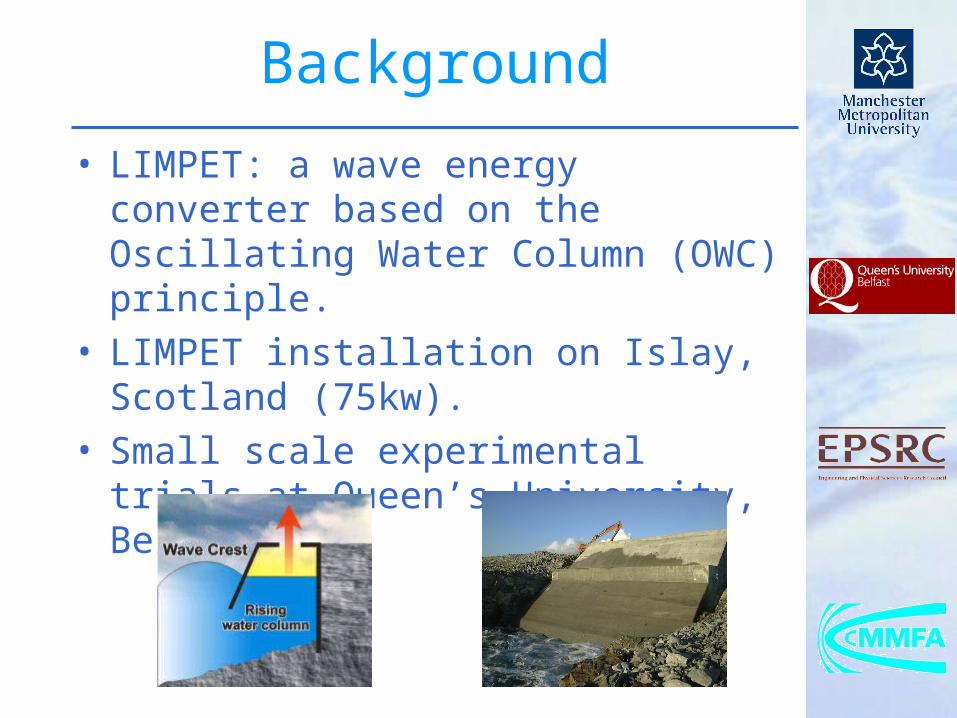
• LIMPET: a wave energy converter based on the Oscillating Water Column (OWC) principle.

• LIMPET installation on Islay, Scotland (75kw).

• Small scale experimental trials at Queen’s University, Belfast.

Background

• The problem involves both water and air flows, wave breaking, non-sinusoidal waves, vortex formation and air entrainment.

• Linear wave theory is not suitable for modelling such flow problems.

• A two-fluid (water/air) non-linear model (Qian,Causon,Ingram and Mingham, Journal of Hydraulic Engineering, Vol.129, no.9, 2003) has been applied in the present study.

AMAZON-SC: Numerical Wave Flume

• Two fluid (air/water), boundary conforming, time accurate, conservation law based, flow code utilising the surface capturing approach.

• Cartesian cut cell techniques are used to represent solid static or moving boundaries.

Governing equations

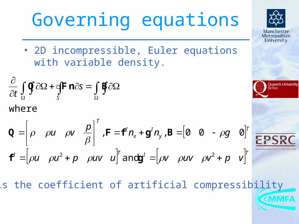
• 2D incompressible, Euler equations with variable density.

TITI

Ty

Ix

I

T

S

vpvuvvuuvpuu

gnnp

vu

st

22 and

000,,

where

.

gf

BgfFQ

BnFQ

is the coefficient of artificial compressibility

Discretisation

• The equations are discretised using a finite volume formulation

Where Qi is the average value of Q in cell i (stored at the cell centre), Vi is the volume of the cell, Fij is the numerical flux across the interface between cells i and j and and lj is the length of side j.

iijikj

jijii RVlt

VQBF

Q

)(

Convective fluxes

• The convective flux (Fij) is evaluated using Roe’s approximate Riemann solver.

• To ensure second order accuracy, MUSCL reconstruction is used

where (x,y) is a point inside the cell ij, r is the coordinate vector of (x,y) relative to ij and Qij is the slope limited gradient.

)(21 ijijij

Iij

IIij QQLRQFQFF

rQQQ ijijyx ),(

Time discretisation

The implicit backward Euler scheme is used together with an artificial time variable (to ensure a divergence free velocity field) and a linearised RHS.

1111111

,1,,1

,11,1,1

where

)(

tttm

mnmnmn

ta

mnmnmn

m

diagI

Rt

VI

RVI

QQQ

QQQ

Q

The resulting system is solved using an approximate LU factorisation.

Computer Implementation

• A Jameson-type dual time iteration is used to eliminate at each real (outer) iteration.

• The code vectorises efficiently with simulations typically taking about three hours to run on an NEC SX6i deskside supercomputer.

Boundary Conditions

• Seaward boundary – a solid moving paddle (boundary) is used to generate waves (wave-maker).

• Atmospheric boundary – a constant atmospheric pressure gradient is applied. Spray and water passing out of this boundary are lost from the computation.

• Landward boundary – a solid wall boundary condition is used for the landward end of the domain.

• Bed and wave power device – modelled using Cartesian cut cell techniques.

Cartesian Cut Cell Method

• Automatic mesh generation

• Boundary fitted

• Extends to moving boundaries

Cartesian Cut Cells

• Input vertices of solid boundary (and domain)

Cartesian Cut Cells

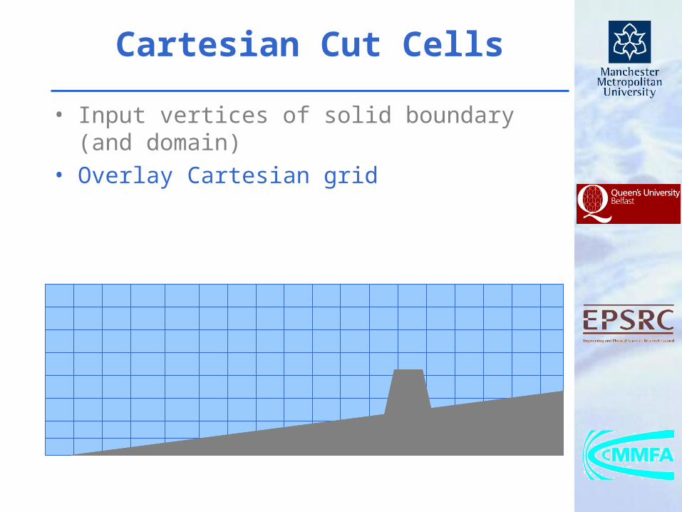
• Input vertices of solid boundary (and domain)• Overlay Cartesian grid

Cartesian Cut Cells

• Input vertices of solid boundary (and domain)• Overlay Cartesian grid

• Identify Cut Cells and compute intersection points.

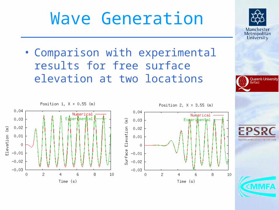
Wave Generation

• Waves are generated using a moving paddle with prescribed velocity: U=-0.2sin(2t)

• 0.3m Still Water Level; 6.0m long wave tank

• Using 120x40 grid cells• 10 waves simulated, starting from still

water

Wave Generation

• Comparison with experimental results for free surface elevation at two locations

LIMPET OWC Simulation

• Wave Conditions: Regular waves with wave length L 1.5m , period T=1.0s and still water level H = 0.15m.

• Device located at about 2 wave lengths from the moving paddle

• 5 seconds simulated, starting from still water

Small Scale Test at QUB

LIMPET OWC Simulation

Free surface position and velocity vectors at T=4.0s

LIMPET OWC Simulation

Free surface position and velocity vectors at T=4.2s

LIMPET OWC Simulation

Free surface position and velocity vectors at T=4.4s

LIMPET OWC Simulation

Free surface position and velocity vectors at T=4.6s

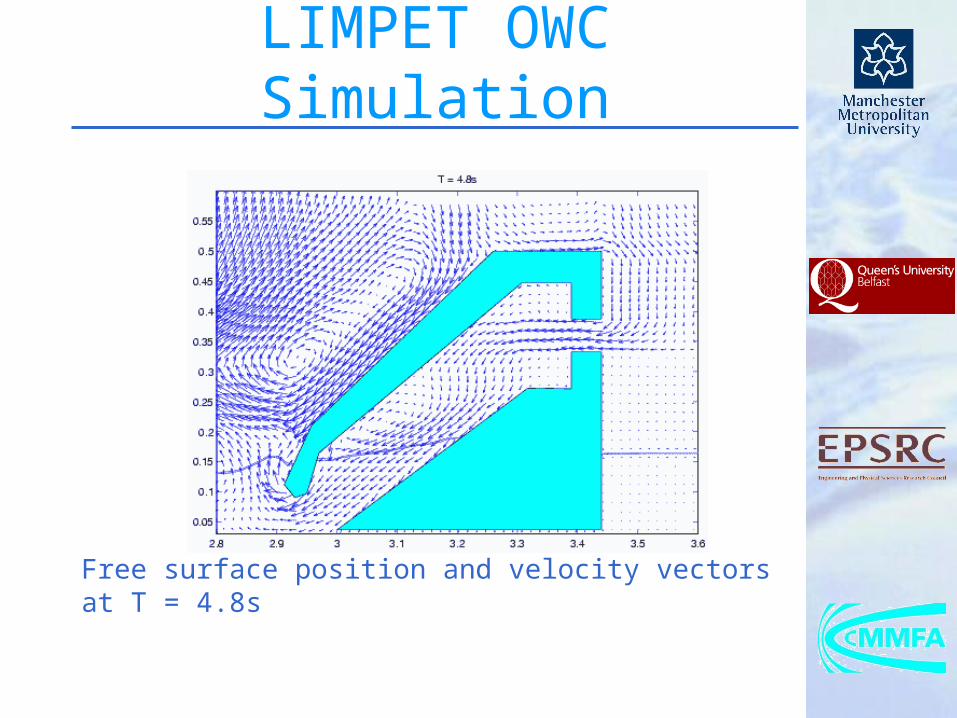
LIMPET OWC Simulation

Free surface position and velocity vectors at T = 4.8s

LIMPET OWC Simulation

Free surface position and velocity vectors at T = 5.0s.

Conclusions

• Some initial results have been presented for simulation of LIMPET OWC device using a surface capturing method in a Cartesian cut cell framework.– The method is computationally efficient,– Capable of modelling both water and air, as well

as their interface – Can handle both static and moving boundary

easily.

• Detailed comparisons with the small scale test from QUB using the same wave conditions are in progress.

• The numerical model is generic and can be used to model a wide range of wave energy devices.