a two-level graph partitioning problem arising in mobile ... · a two-level graph partitioning...
TRANSCRIPT

A Two-Level Graph Partitioning Problem Arising
in Mobile Wireless Communications
Jamie Fairbrother∗ Adam N. Letchford† Keith Briggs‡
To appear in Computational Optimization and Applications
Abstract
In the k-partition problem (k-PP), one is given an edge-weighted undirected graph,and one must partition the node set into at most k subsets, in order to minimise (ormaximise) the total weight of the edges that have their end-nodes in the same clus-ter. Various hierarchical variants of this problem have been studied in the contextof data mining. We consider a ‘two-level’ variant that arises in mobile wireless com-munications. We show that an exact algorithm based on intelligent preprocessing,cutting planes and symmetry-breaking is capable of solving small- and medium-sizeinstances to proven optimality, and providing strong lower bounds for larger in-stances.
Keywords: graph partitioning, integer programming, cutting planes, telecommu-nications.
1 Introduction
Telecommunications has proven to be a rich source of interesting optimisation problems[38]. In the case of wireless communications, the hardest (and most strategic) problem iswireless network design, which involves the simultaneous determination of cell locationsand shapes, base station locations, power levels and frequency channels (e.g., [32]).On a more tactical level, one finds various frequency assignment problems, which areconcerned solely with the assignment of available frequency bands to wireless devices(e.g., [1]).
A rather different optimisation problem arises in the context of mobile wireless com-munications. The technology is the 4G (LTE) standard, and the essence of the problemis as follows. There are a number of cells with known locations, and each cell must beassigned a positive integer identifier before it can operate. In the LTE standard, thisis called a Physical Cell Identifier or PCI, but to keep the discussion general we willsimply use the term ID. If two cells are close to each other (according to some measureof closeness), they are said to be neighbours. Two neighbouring cells must not have thesame ID. We are also given two small integers k, k′, both greater than two. If the IDs
∗STOR-i Centre for Doctoral Training, Lancaster University, Lancaster LA1 4YF, UK. E-mail:[email protected]†Department of Management Science, Lancaster University, Lancaster LA1 4YW, United Kingdom.
E-mail: [email protected]‡Wireless Research Group, BT Technology, Service & Operations, Martlesham Heath, UK. Email:
1
of two neighbouring devices are the same modulo k, it causes interference. Moreover,some additional interference occurs (but at a lesser level) if they are the same modulokk′. Typical values are k=3 and k′=2, and the interferences arise because of the wayreference signals (containing the ID) are encoded into a channel broadcast by the cells.The net effect is that devices wanting to connect to cells cannot do this successfully ifthey cannot decode the reference signals because of interference. The overall task is thusto assign IDs to devices in such a way as to minimise the total interference.
The problem turns out to be a generalisation of a well-known NP-hard combinatorialoptimisation problem called the k-partition problem or k-PP. For reasons which willbecome clear later, we call it the 2-level partition problem or 2L-PP. In real-life LTEsystems, the 2L-PP is typically solved approximately, via simple distributed heuristics.These heuristics perform adequately at present, but they may prove inadequate in future,as devices proliferate. To test the quality of alternative heuristics, it is necessary to haveproven optimal solutions, or at least strong lower bounds, for a collection of realisticinstances. For this reason, we developed an exact algorithm for the 2L-PP, based oninteger programming. This algorithm turns out to be capable of solving small - andmedium-sized 2L-PP instances to proven optimality, and providing strong lower boundsfor larger instances.
The structure of the paper is as follows. In Section 2, the literature on the k-PPis reviewed. In Section 3, we formulate our problem as an integer program (IP) andderive some valid linear inequalities (i.e. cutting planes). In Section 4, we describe ourexact algorithm in detail. In Section 5, we describe some computational experimentsand analyse the results. Finally, some concluding remarks are made in Section 6.
2 Literature Review
Since the 2L-PP is a generalisation of the k-PP, we now review the literature on thek-PP. We define the k-PP in Section 2.1. The main IP formulations are presented inSection 2.2. The remaining two subsections cover cutting planes and algorithms forgenerating them, respectively.
We remark that some other multilevel graph partitioning problems have been studiedin the data mining literature; see, e.g., [8, 40, 13, 39]. In those problems, however,neither the number of clusters nor the number of levels is fixed. For this reason, we donot consider them further.
2.1 The k-partition problem
The k-PP was first defined in [7]. We are given a (simple, loopless) undirected graphG, with vertex set V ={1, . . . , n} and edge set E, a rational weight we for each edgee∈E, and an integer k with 26k6n. The task is to partition V into k or fewer subsets,such that the sum of the weights of the edges that have both end-vertices in the samecluster is minimised. In the context of this work, it is more intuitive to interpret this asa colouring problem: each node must be assigned one of k colours, two adjacent nodes
2

(i.e. two nodes linked by an edge) having the same colour constitutes a conflict, and theaim is to minimize the weighted sum of conflicts.
The k-PP has applications in scheduling, statistical clustering, numerical linear alge-bra, telecommunications, VLSI layout and statistical physics (see, e.g., [7, 18, 21, 37]).It is strongly NP-hard for any fixed k>3, since it includes as a special case the problemof testing whether a graph is k-colourable. It is also strongly NP-hard when k=2, sinceit is then equivalent the well-known max-cut problem, and when k=n, since it is thenequivalent to the clique partitioning problem [23, 24].
2.2 Formulations of the k-PP
Chopra & Rao [9] present two different IP formulations for the k-PP. In the first formu-lation, there are two sets of binary variables. For each v∈V and for c=1, . . . , k, let xvcbe a binary variable, taking the value 1 if and only if vertex v has colour c. For eachedge e∈E, let ye be an additional binary variable, taking the value 1 if and only if bothend-nodes of e have the same colour. Then we have the following optimization problem:
min∑
e∈E weye
s.t.∑k
c=1 xvc=1 (v∈V ) (1)
yuv>xuc+xvc−1 ({u, v}∈E, c=1, . . . , k) (2)
xuc>xvc+yuv−1 ({u, v}∈E, c=1, . . . , k) (3)
xvc>xuc+yuv−1 ({u, v}∈E, c=1, . . . , k) (4)
xvc∈{0, 1} (v∈V, c=1, . . . , k)
yuv∈{0, 1} ({u, v}∈E).
The equations (1) force each node to be given exactly one colour, and the constraints(2)–(4) ensure that the y variables take the value 1 when they are supposed to. Notethat constraints (3) and (4) can be dropped in the case where we>0 for all e∈E.
This IP has O(m+nk) variables and constraints, where m=|E|. It therefore seemssuitable when k is small and G is sparse. Unfortunately, it has a very weak linearprogramming (LP) relaxation. Indeed, if we set all x variables to 1/k and all y variablesto 0, we obtain the trivial lower bound of 0. Moreover, it suffers from symmetry, in thesense that given any feasible solution, there exist k! solutions of the same cost. (SeeMargot [33] for a tutorial and survey on symmetry issues in integer programming.)
The second IP formulation is obtained by dropping the x variables, but having a yvariable for every pair of nodes, setting wuv to zero if {u, v} /∈E. Then:
min∑
e∈E weye
s.t.∑
u,v∈C yuv>1 (C⊂V :|C|=k+1) (5)
yuv>yuw+yvw−1 ({u, v, w}⊂V ) (6)
yuv∈{0, 1} ({u, v}⊂V ).
The constraints (5), called clique inequalities, ensure that, in any set of k+1 nodes, atleast two receive the same colour. The constraints (6) enforce transitivity; that is, if
3

nodes u and w have the same colour, and nodes v and w have the same colour, thennodes u and v must also have the same colour.
A drawback of the second IP formulation is that it has O(n2) variables and O(nk+1)constraints, and it cannot exploit any special structure that G may have (such as spar-sity).
A third IP formulation, based on so-called representatives, is studied in [2]. Therealso exist several semidefinite programming relaxations of the k-PP (see, e.g., [20, 18,21, 37, 3, 42, 30]). For the sake of brevity we do not go into details.
2.3 Cutting planes
Chopra & Rao [9] present several families of valid linear inequalities (i.e. cutting planes),which can be used to strengthen the LP relaxation of the above formulations. For ourpurposes, the most important turned out to be the generalised clique inequalities, whichprovide a lower bound on the number of conflicts for any clique with more than k nodes.In the case of the first IP formulation, they take the form∑
u,v∈Cyuv >
(t+1
2
)r+
(t
2
)(k−r), (7)
where C⊆V is a clique (set of pairwise adjacent nodes) in G with |C|>k, and t and rdenote
⌊|C|/k
⌋and r=|C| mod k, respectively. In the case of the second IP formulation,
they must be defined for any C⊆V with |C|>k (since every set of nodes forms a cliquein a complete graph). In either case, they define facets of the associated polytope whenk>3 and r 6=0. Note that they reduce to the clique inequalities (5) when |C|=k+1.
Further inequalities for the first IP formulation can be found in [9, 30]. Furtherinequalities for the second formulation can be found in, e.g., [24, 15, 16, 9, 10, 36].
2.4 Separation algorithms
For a given family of valid inequalities, a separation algorithm is an algorithm whichtakes an LP solution and searches for violated inequalities in that family [22].
By brute-force enumeration, one can solve the separation problem for the inequali-ties (2)–(4) in O(km) time, for the transitivity inequalities (6) in O
(n3)
time, and forthe clique inequalities (5) in O
(nk+1
)time. It is stated in [9] that separation of the
generalised clique inequalities (7) is NP-hard. An explicit proof, using a reduction fromthe max-clique problem, is given in [17]. Heuristics for clique and generalised cliqueseparation are presented in [17, 28].
Separation results for other inequalities for the first IP formulation can be found in[9, 30]. Separation results for the second formulation can be found in, e.g.,[23, 16, 6, 4,36, 29, 35]. For some computational results with various separation algorithms, see [14].
4
3 Formulation and Valid Inequalities
In this section, we give an IP formulation of the 2L-PP (Section 3.1) and derive somevalid inequalities (3.2). We also show how to modify the formulation to address issuesof symmetry (3.3).
3.1 Integer programming formulation
In order to demonstrate that the 2L-PP is a generalisation of the k-PP, we presentthe problem in its most general form, before describing how this is used to model ourtelecommunications problem. An instance of the 2L-PP is given by an undirected graphG=(V,E), integers k, k′>2, and two sets of edge weights we, w
′e∈R for e∈E. The 2L-PP
is a type of node colouring problem with colours {0, . . . , kk′−1} and where two types ofconflicts may occur: a modulo k conflict occurs if two adjacent nodes are assigned thesame colour up to modulo k, and a modulo kk′ conflict occurs if two adjacent nodes useexactly the same colour. The aim of the 2L-PP is to find a colouring which minimizesthe sum of modulo k conflicts weighted by (we)e∈E , plus the sum of modulo kk′ conflictsweighted by (w′e)e∈E .
To formulate the 2L-PP as an IP, we modify the first formulation mentioned inSection 2.2. We have three sets of binary variables. For each v∈V and for c=0, . . . , kk′−1,let xvc be a binary variable, taking the value 1 if and only if vertex v has colour c. Foreach edge e∈E, define two binary variables ye and ze, taking the value 1 if and only ifboth end-nodes of e have the same colour modulo k, or the same colour, respectively.Then we have:
min∑{u,v}∈E (weyuv+w′ezuv) (8)
s.t.∑kk′−1
c=0 xvc=1 (v∈V ) (9)
yuv>∑k′−1
r=0 xu,c+rk+∑k′−1
r=0 xv,c+rk−1 ({u, v}∈E, c=0, . . . , k−1) (10)∑k′−1r=0 xu,c+rk>yuv+
∑k′−1r=0 xv,c+rk−1 ({u, v}∈E, c=0, . . . , k−1) (11)∑k′−1
r=0 xv,c+rk>yuv+∑k′−1
r=0 xu,c+rk−1 ({u, v}∈E, c=0, . . . , k−1) (12)
zuv>xuc+xvc−1 ({u, v}∈E, c=0, . . . , kk′−1) (13)
xuc>zuv+xvc−1 ({u, v}∈E, c=0, . . . , kk′−1) (14)
xvc>zuv+xuc−1 ({u, v}∈E, c=0, . . . , kk′−1) (15)
xvc∈{0, 1} (v∈V, c=0, . . . , kk′−1) (16)
yuv, zuv∈{0, 1} ({u, v}∈E). (17)
The objective function (8) is just a weighted sum of the two kinds of colour con-flicts. The constraints (9) state that each node must have a unique colour. The con-straints (10)–(12) ensure (ye)e∈E indicate modulo k colour conflicts while (13)–(15) en-sure (ze)e∈E indicate modulo kk′ conflicts. The remaining constraints are just binary
5

conditions. In the above formulation, when k′=1 the constraints (10)–(15) force thevariables ye and ze to be equal for all e∈E, and so the problem becomes a k-PP.
Our telecommunications application is modelled by the 2L-PP as follows: each nodein V corresponds to a device, and a pair of nodes is connected by an edge if and only ifthe corresponding devices are neighbours; assigning the colour c to a node corresponds togiving the corresponding device an ID that is congruent to c modulo kk′; the weights ofeach type of conflict constant and are given by positive numbers w and w′ which specifythe relative importance given to interference modulo k and modulo kk′, respectively;finally the aim of the problem is to minimize the weighted sum of the two kinds ofinterference. As in the case of the k-PP, the positive edge weights render some of theconstraints of the above formulation redundant, in particular (11), (12), (14) and (15).Note that the above IP has kk′n+2m variables and n+3k(k′+1)m linear constraintsand so for sparse graphs and small values k and k′, which characterise our application,this formulation is manageable.
An intuitive approach to solving the 2L-PP would be to first solve the k-PP, and thensolve the k′-PP for each of the k subgraphs induced by nodes of the same colour, usingappropriate weights at each stage. However, this method does not necessarily yield anoptimal solution with respect to the above formulation even in the case where we haveconstant positive edge weights as in our application. This is because there may existsubstantial flexibility in the topologies of the k induced subgraphs which minimize thenumber of modulo k conflicts, and these different topologies may have different optimalnumbers of k′ conflicts. Therefore, optimizing modulo k conflicts first will not necessarilyyield subgraphs which produce an optimal weighted sum of modulo k and kk′ conflicts.In the case where edge weights vary independently for each type of conflict, this heuristicmay perform even worse as a subgraph induced by nodes of the same colour modulo kwhich has small modulo k weights, may have large modulo kk′ weights.
3.2 Valid inequalities
Unfortunately, our IP formulation of the 2L-PP shares the same drawbacks as the firstformulation of the k-PP mentioned in Section 2.2: it has a very weak LP relaxation(giving a trivial lower bound of zero), and it suffers from a high degree of symmetry.
To strengthen the LP relaxation, we add valid linear inequalities from three families.For a clique C⊂V , let y(C) and z(C) denote
∑{u,v}⊂C yuv and
∑{u,v}⊂C zuv, respectively.
The first two families of inequalities are straightforward adaptations of the generalisedclique inequalities (7) for the k-PP. Specifically, given a clique C, the inequalities (18)and (19) give lower bounds on the number of modulo k and modulo kk′ conflicts whichany colouring must induce.
Proposition 3.1 The following inequalities are satisfied by all feasible solutions of the2L-PP:
• “y-clique” inequalities, which take the form:
y(C)>
(t+1
2
)r+
(t
2
)(k−r), (18)
6

where C⊆V is a clique with |C|>k, t=b|C|/kc and r=|C| mod k;
• “z-clique” inequalities, which take the form:
z(C)>
(T+1
2
)R+
(T
2
)(kk′−R), (19)
where C⊆V is a clique with |C|>kk′, T=⌊|C|kk′
⌋and R=|C| mod kk′.
Proof. This follows from the result of Chopra & Rao [9] mentioned in Section 2.3,together with the fact that, in a feasible IP solution, the y and z vectors are the incidencevectors of a k-partition and a kk′-partition, respectively. �
The third family of inequalities, which is completely new, is described in the followingtheorem. These inequalities follow from the fact that a kk′ colouring induces a partitionof a clique into k subcliques of the same colours modulo k, and each of these subcliquesmust have at least a given number of modulo k′ conflicts.
Theorem 3.1 For all cliques C⊆V with |C|>k′, the following “(y, z)-clique” inequalitiesare valid:
k′ z(C)>y(C)−t′(k′
2
)−(r′
2
), (20)
where t′=b|C|/k′c and r′=|C| mod k′.
Proof. See the Appendix. �
The following two lemmas and theorem give necessary conditions for the inequalitiespresented so far to be facets (i.e., not implied by other inequalities).
Lemma 3.1 A necessary condition for the y-clique inequality (18) to be a facet is thatr 6=0.
Proof. This was already shown by Chopra & Rao [9]. �
Lemma 3.2 A necessary condition for the (y, z)-clique inequality (20) to be facet is thatr′ 6=0.
Proof. Suppose that r′=0. The (y, z)-clique inequality for C can be written as:
k′ z(C)>y(C)−|C|(k′−1)/2. (21)
Now let v be an arbitrary node in C. The (y, z)-clique inequality for the set C\{v} canbe written as:
k′ z(C\{v})>y(C\{v})− (|C|−2)(k′−1)/2.
Summing this up over all v∈C yields
k′(|C|−2) z(C)>(|C|−2) y(C)− |C|(|C|−2)(k′−1)/2.
Dividing this by |C|−2 yields the inequality (21). �
7

Theorem 3.2 A necessary condition for the z-clique inequality (19) to be a facet is that1<R<kk′−1.
Proof. See the Appendix. �
Our experiments with the polyhedron transformation software package PORTA [11]lead us to make the following conjecture:
Conjecture 3.1 The following results hold for the convex hull of 2L-PP solutions:
• y-clique inequalities (7) define facets if and only if r 6=0.
• z-clique inequalities (19) define facets if and only if 1<R<kk′−1.
• (y, z)-clique inequalities (20) define facets if and only if r′ 6=0.
In any case, we have found that all three families of inequalities work very well in practiceas cutting planes. Moreover, in our preliminary experiments, we found that the y-cliqueinequalities were the most effective at improving the lower bound, with the yz-cliqueinequalities being the second most effective.
Remark: The trivial inequality ye>ze is also valid for all e∈E. In our preliminaryexperiments, however, these inequalities proved to be of no value as cutting planes.
3.3 Symmetry
Another issue to address is symmetry. Note that any permutation σ on the set of colours{0, . . . , kk′−1} such that σ(c) mod k=c mod k will preserve all k and kk′ conflicts. Sincethere are k′! such permutations, for any colouring (which makes use of all availablecolours) there are at least k′! other colourings which yield the same cost.
One easy way to address this problem, at least partially, is given in the followingtheorem:
Theorem 3.3 For any colour c∈{0, . . . , kk′−1}, let φ(c) denote bc/kc+(c mod k). Then,one can fix to zero all variables xvc for which φ(c)>v, while preserving at least one op-timal 2L-PP solution.
Proof. See the Appendix. �
Example: Suppose that n>4 and k=k′=3. Then φ(0), . . . , φ(8) are 0, 1, 2, 1, 2, 3, 2,3 and 4, respectively. So we can fix the following variables to zero: x11, . . . , x18; x22;x24, . . . , x28; x35, x37, x38 and x48. �
4 Exact Algorithm
We now describe an exact solution algorithm for the 2L-PP. The algorithm consistsof two main stages: preprocessing and cut-and-branch. Preprocessing is described inSection 4.1, while the cut-and-branch algorithm is described in Section 4.2. Throughoutthis section, for a given set of nodes V ′⊆V , we let G[V ′] denote the subgraph of Ginduced by the nodes in V ′.
8

xxx
xxx
xxx
xxx
xxx
�������
@@@@
@@@@
����
����@
@@@
xx
xx
xx x
xxx
����@@@@
@@@@
����
����@
@@@
Figure 1: A graph (left) and its (unique) 3-core (right).
4.1 Preprocessing
In the first stage, an attempt is made to simplify the input graph G and, if possible,decompose it into smaller and simpler subgraphs. This is via two operations, whichwe call k-core reduction and block decomposition. Although we focus on the 2L-PP thefollowing results also apply to the k-PP.
A k-core of a graph G is a maximal connected subgraph whose nodes all have degreeof at least k. The concept was first introduced in [41], as a tool to measure cohesion insocial networks. An example is given in Fig. 1, but it should be borne in mind that, ingeneral, a graph may have several (node-disjoint) k-cores. The k-cores of a graph canbe found easily, in O
(n2)
time, via a minor adaptation of an algorithm given in [43].Details are given in Algorithm 1.
Algorithm 1: Algorithm for finding k-cores of a graph
input : graph G=(V,E)output: k-cores of GV ′ :=V ;do
Let V − equal{v∈V ′ : degG[V ′] (v)<k
};
if V − 6=∅ thenV ′ :=V ′\V −;
end
while V − 6=∅;Output the connected components of G[V ′]
The reason that k-cores are of interest is given in the following proposition:
Proposition 4.1 For any graph G, and non-negative edge weights we and w′e for e∈E,the cost of the optimal 2L-PP solution is equal to the sum of the costs of the optimalsolutions of the 2L-PP instances given by its k-cores.
Proof (sketch). Let v∈V be any node whose degree in G is less than k. Suppose wesolve the 2L-PP on the induced subgraph G[V \{v}]. Then we can extend the 2L-PP
9
xx
xx
xx
����@
@@@
@@@@
x xx
xx
����
����@@@@
xx
xx
����@
@@@
xx
xx
����@
@@@
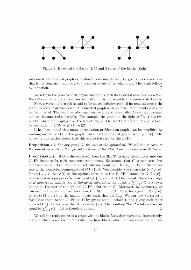
Figure 2: Blocks of the 3-core (left) and 3-cores of the blocks (right).
solution to the original graph G, without increasing its cost, by giving node v a colourthat is not congruent modulo k to the colour of any of its neighbours. The result followsby induction. �
We refer to the process of the replacement of G with its k-core(s) as k-core reduction.We will say that a graph is k-core reducible if it is not equal to the union of its k-cores.
Now, a vertex of a graph is said to be an articulation point if its removal causes thegraph to become disconnected. A connected graph with no articulation points is said tobe biconnected. The biconnected components of a graph, also called blocks, are maximalinduced biconnected subgraphs. For example, the graph on the right of Fig. 1 has twoblocks, which are displayed on the left of Fig. 2. The blocks of a graph G=(V,E) canbe computed in O(|V |+|E|) time [27].
It has been noted that many optimisation problems on graphs can be simplified byworking on the blocks of the graph instead of the original graph; see, e.g., [26]. Thefollowing proposition shows that this is also the case for the 2L-PP.
Proposition 4.2 For any graph G, the cost of the optimal 2L-PP solution is equal tothe sum of the costs of the optimal solutions of the 2L-PP instances given by its blocks.
Proof (sketch). If G is disconnected, then the 2L-PP trivially decomposes into one2L-PP instance for each connected component. So assume that G is connected butnot biconnected. Let v∈V be an articulation point, and let V1, . . . , Vt be the vertexsets of the connected components of G[V \{v}]. Now consider the subgraphs G[Vi∪{v}]for i=1, . . . , t. Let S(i) be the optimal solution to the 2L-PP instance on G[Vi∪{v}],represented as a proper kk′-colouring of Vi∪{v}, and let c(i) be its cost. Since each edgeof E appears in exactly one of the given subgraphs, the quantity
∑ti=1 c(i) is a lower
bound on the cost of the optimal 2L-PP solution on G. Moreover, by symmetry, wecan assume that node v receives colour 1 in S(1), . . . , S(t). Now, for a given u∈V \{v},let i(u)∈{1, . . . , t} be the unique integer such that u∈Vi(u). We can now construct afeasible solution to the 2L-PP on G by giving node v colour 1, and giving each othernode u∈V \{v} the colour that it has in S(i(u)). The resulting 2L-PP solution has costequal to
∑ti=1 c(i), and is therefore optimal. �
We call the replacement of a graph with its blocks block decomposition. Interestingly,a graph which is not k-core reducible may have blocks which are; see again Fig. 2. This
10
leads us to apply k-core reduction and block decomposition recursively, until no morereduction or decomposition is possible.
At the end of this procedure, we have a collection of induced subgraphs of G whichare biconnected and not k-core reducible, and we can solve the 2L-PP on each sub-graph independently. Given the optimal solutions for each subgraph, we can reconstructan optimal solution for the original graph by recursively constructing solutions for thepredecessor graph of a reduction or decomposition.
4.2 Cut-and-branch algorithm
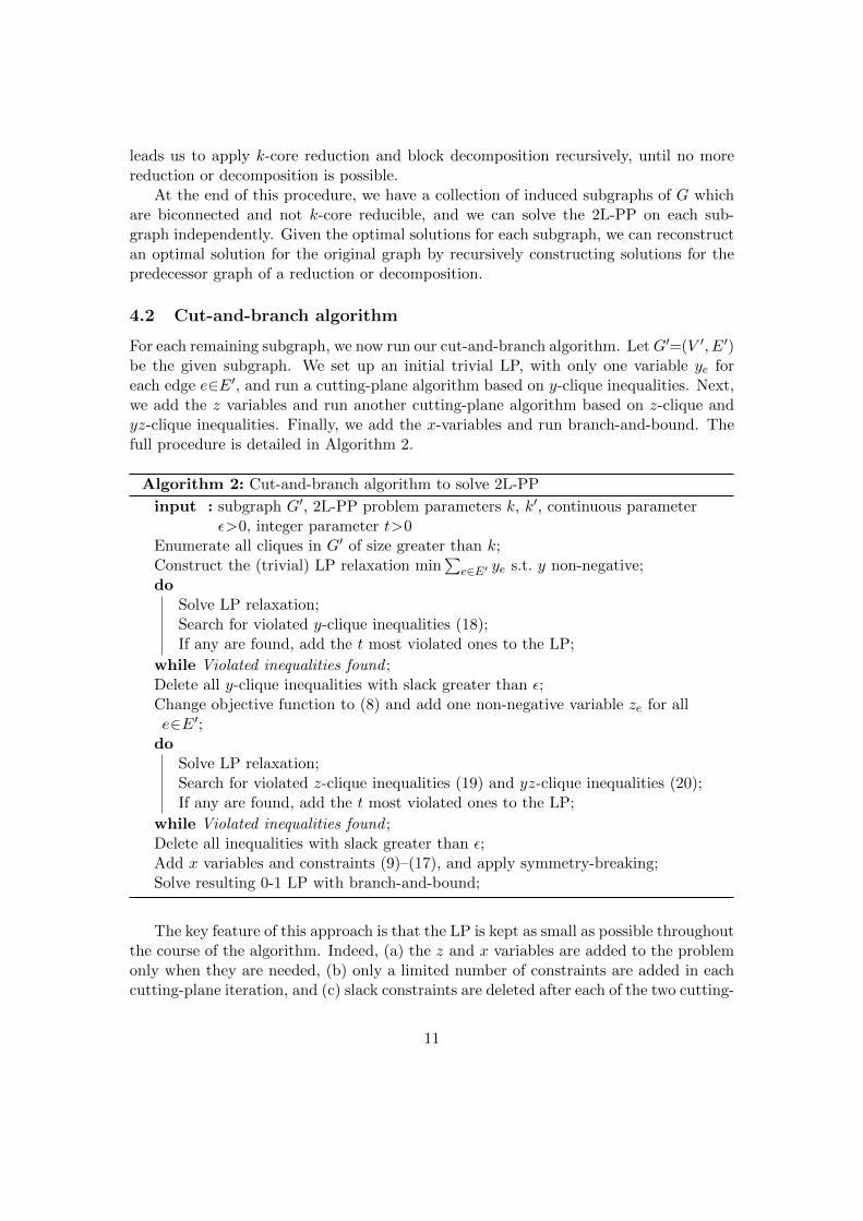
For each remaining subgraph, we now run our cut-and-branch algorithm. LetG′=(V ′, E′)be the given subgraph. We set up an initial trivial LP, with only one variable ye foreach edge e∈E′, and run a cutting-plane algorithm based on y-clique inequalities. Next,we add the z variables and run another cutting-plane algorithm based on z-clique andyz-clique inequalities. Finally, we add the x-variables and run branch-and-bound. Thefull procedure is detailed in Algorithm 2.
Algorithm 2: Cut-and-branch algorithm to solve 2L-PP
input : subgraph G′, 2L-PP problem parameters k, k′, continuous parameterε>0, integer parameter t>0
Enumerate all cliques in G′ of size greater than k;Construct the (trivial) LP relaxation min
∑e∈E′ ye s.t. y non-negative;
doSolve LP relaxation;Search for violated y-clique inequalities (18);If any are found, add the t most violated ones to the LP;
while Violated inequalities found ;Delete all y-clique inequalities with slack greater than ε;Change objective function to (8) and add one non-negative variable ze for alle∈E′;do
Solve LP relaxation;Search for violated z-clique inequalities (19) and yz-clique inequalities (20);If any are found, add the t most violated ones to the LP;
while Violated inequalities found ;Delete all inequalities with slack greater than ε;Add x variables and constraints (9)–(17), and apply symmetry-breaking;Solve resulting 0-1 LP with branch-and-bound;
The key feature of this approach is that the LP is kept as small as possible throughoutthe course of the algorithm. Indeed, (a) the z and x variables are added to the problemonly when they are needed, (b) only a limited number of constraints are added in eachcutting-plane iteration, and (c) slack constraints are deleted after each of the two cutting-
11
plane algorithms has terminated. The net result is that both cutting-plane algorithmsrun very efficiently, and so does the branch-and-bound algorithm at the end.
We now make some remarks about the separation problems for the three kinds ofclique inequalities. Since all three separation problems seem likely to be NP-hard, weinitially planned to use greedy separation heuristics, in which the set C is enlarged onenode at a time. We were surprised to find, however, that it was feasible to solve theseparation problems exactly, by brute-force enumeration, for typical 2L-PP instancesencountered in our application. The reason is that the original graph G tends to befairly sparse in practice, and each subgraph G′ generated by our preprocessor tends tobe fairly small. Accordingly, after the preprocessing stage, we use the Bron-Kerboschalgorithm [5] to enumerate all maximal cliques in each subgraph G′. It is then fairlyeasy to solve the separation problems by enumeration, provided that one takes care notto examine the same clique twice in a given separation call. We omit details, for brevity.
We remark that, although an arbitrary graph with n nodes can have as many as 3n3
maximal cliques [34], a graph in which all nodes have degree at most d can have at most
(n−d)3d3 of them [19].
5 Computational Experiments
We now present the results of some computational experiments. In Section 5.1, wedescribe how we constructed the graphs used in our experiments. In Section 5.2, we testthe preprocessing algorithm for different values of k. In Section 5.3 we study the effectof our symmetry-breaking constraints on the required solution time. In Section 5.4, wepresent results on our the cut-and-branch algorithms.
Throughout these experiments, the value of k varies between 2 and 5, while forsimplicity, we fix k′=2, since the value of k′ does not affect the performance of thegraph preprocessing algorithm. All experiments have been run on a high performancecomputer with an Intel 2.6 GHz processor and using 16 cores. Graph preprocessing andclique enumeration was done using igraph [12] and the linear and integer programs weresolved using Gurobi v.7.5 [25]. All ILP instances are given a time limit of three hours tobe solved. Unless otherwise stated we use the default for all other of Gurobi’s settings.
5.1 Graph construction
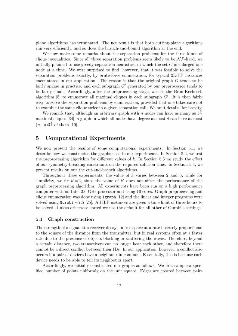
The strength of a signal at a receiver decays in free space at a rate inversely proportionalto the square of the distance from the transmitter, but in real systems often at a fasterrate due to the presence of objects blocking or scattering the waves. Therefore, beyonda certain distance, two transceivers can no longer hear each other, and therefore therecannot be a direct conflict between their IDs. In our application, however, a conflict alsooccurs if a pair of devices have a neighbour in common. Essentially, this is because eachdevice needs to be able to tell its neighbours apart.
Accordingly, we initially constructed our graphs as follows. We first sample a spec-ified number of points uniformly on the unit square. Edges are created between pairs
12

(a) Edges are created be-tween nodes within a givenradius of each other
(b) Graph is augmented withedges between nodes whichhave a neighbour in common
Figure 3: Construction of neighbourhood graph
of points if they are within a specified radius of each other. This yields a so-called diskgraph; see, e.g., [31]. The graph is then augmented with edges between pairs of nodeswhich have a neighbour in common. (In other words, we take the square of the diskgraph.) This construction is illustrated in Figure 3.
It turned out, however, that neighbourhood graphs constructed in this way yieldedextremely easy 2L-PP instances. The reason is that nodes near to the boundary ofthe square tend to have small degree, which causes them to be removed during thepreprocessing stage. This in turn causes their neighbours to have small degree, and soon. In order to create more challenging instances, and to avoid this “boundary effect”,we decided to use a torus topology to calculate distances between points in the unitsquare before constructing the graphs.
5.2 Preprocessing
In order to understand the potential benefits of the preprocessing stage, we have cal-culated the effect of preprocessing on our random neighbourhood graphs for differentvalues of k and disk radius, while fixing n=100. In particular, for radius 0.01, . . . , 0.2 andk=3, 4, 5, we calculate the mean proportion of edges eliminated and the mean proportionof vertices in the largest remaining component. The results are shown in Figure 4. Themeans were estimated by simulating 1000 random graphs for each pair of parameters.
The results show that, for all values of k, the proportion of edges eliminated decaysto zero rather quickly as the disk radius is increased. The proportion of nodes in thelargest component also tends to one as the radius is increased, but at a slower rate thanthe convergence for edge reduction.
In order to gain further insight, we also explored how the average degree in ourrandom neighbourhood graphs depends on the number of nodes and the disk radius.The results are shown in Figure 5. A comparison of this figure and the preceding oneindicates that, as one might expect, preprocessing works best when the average degreeis not much larger than k.
13

0.05
0.10
0.15
0.20
Disk radius
0.0
0.2
0.4
0.6
0.8
1.0
Edge R
educt
ion
0.05
0.10
0.15
0.20
Disk radius
0.0
0.2
0.4
0.6
0.8
1.0
Maxim
um
Vert
ices
k = 3k = 4k = 5
Figure 4: Preprocessing of random neighbourhood graphs
5.3 Symmetry constraints
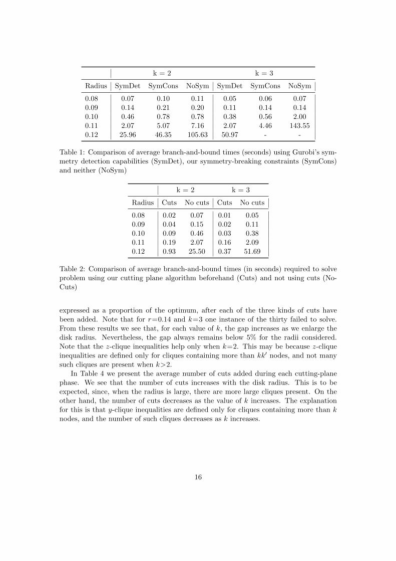
In this numerical experiment we gauge the utility of our symmetry-breaking constraintsby looking at the branch-and-bound time required to solve the 2L-PP. In particular,we compare the times required for solution using our symmetry-breaking constraints,using Gurobi’s symmetry detection capabilities, and using neither symmetry detectionnor symmetry-breaking constraints.
For n=100, and for disk radii ranging from 0.08 to 0.12, we construct 30 randomneighbourhood graphs. The same sets of points were used to construct the graphs foreach disk radius. We also considered two values of k, namely 2 and 3. The weightsw,w′ were both set to 1 for simplicity. For each of the resulting 300 2L-PP instances,we run branch-and-bound with preprocessing but no cutting planes. When solvingthe problems using our symmetry-breaking constraints, we disable Gurobi’s symmetrydetection capabilities.
The results are shown in Table 1. A dash means that at least one instance failedto solve for that radius and value of k. In this experiment one instance out of thethirty failed to solve within the given time limit for r=0.12 and k=3 when we usedour symmetry-breaking constraints, and four failed to solve for the same radius whenneither symmetry-breaking constraint nor symmetry detection were used. These resultsdemonstrate that using our symmetry-breaking constraints, in general, significantly re-duces the solution time required to solve the problem compared to using the Gurobisolver with symmetry detection capabilities switched off, and this benefit increases asthe graphs become dense. However, Gurobi’s symmetry detection capabilities generallyoutperform just using our symmetry-breaking constraints. This indicates that theseconstraints will generally only be useful for MIP solvers which do not have sophisti-cated symmetry-detection algorithms. In order to test our methodology for more densegraphs, we will therefore use Gurobi’s symmetry detection capabilities rather than oursymmetry-breaking constraints.
14

0.00
0.02
0.04
0.06
0.08
0.10
0.12
0.14
0.16
Disk radius
0
2
4
6
8
10
Avera
ge d
egre
e
n = 50n = 100n = 150n = 200
Figure 5: Mean average degree of random neighbourhood graphs
5.4 Cutting planes
Next, we present two numerical experiments on the effectiveness of using our cuttingplanes. In first experiment, we compare the branch-and-bound time required to solve the2L-PP problems using and not using our cutting plane algorithm beforehand. We solvethe exact same 300 problems as were used in the previous experiment, and preprocessthe graphs before solving the problem. Note that we do not take into the time of thecutting plane algorithm in this comparison. As the next experiment shows, the cuttingplane time is negligible compared to the branch-and-bound time.
The results for this first experiment are shown in Table 2. These demonstrate thatusing our cutting planes reduces the solution time required dramatically, and by an orderof magnitude for harder problems.
In the final experiment, we study the lower bounds yielded by each phase of thecutting plane algorithm, and the times these take to run. In this experiment, we usethe previously constructed problems, and in addition construct more difficult problems,which may not have been solvable in the previous experiments. For the disk radii 0.13and 0.14 we construct another 30 problems. In addition, we also solve the 2L-PP for k=4for all constructed graphs, as this problem will be non-trivial for the new denser graphs.For each of the resulting 630 2L-PP instances, we run the preprocessing algorithm,followed by the cut-and-branch algorithm.
In order to measure the effects of the yz-clique and the z-clique inequalities, wehave divided the second cutting-plane phase into two sub-phases, whereby yz-cliqueinequalities are added in the first subphase and z-clique inequalities are added in thesecond subphase.
In Table 3, we present the average gap between the lower bound and optimum,
15
k = 2 k = 3
Radius SymDet SymCons NoSym SymDet SymCons NoSym
0.08 0.07 0.10 0.11 0.05 0.06 0.070.09 0.14 0.21 0.20 0.11 0.14 0.140.10 0.46 0.78 0.78 0.38 0.56 2.000.11 2.07 5.07 7.16 2.07 4.46 143.550.12 25.96 46.35 105.63 50.97 - -
Table 1: Comparison of average branch-and-bound times (seconds) using Gurobi’s sym-metry detection capabilities (SymDet), our symmetry-breaking constraints (SymCons)and neither (NoSym)
k = 2 k = 3
Radius Cuts No cuts Cuts No cuts
0.08 0.02 0.07 0.01 0.050.09 0.04 0.15 0.02 0.110.10 0.09 0.46 0.03 0.380.11 0.19 2.07 0.16 2.090.12 0.93 25.50 0.37 51.69
Table 2: Comparison of average branch-and-bound times (in seconds) required to solveproblem using our cutting plane algorithm beforehand (Cuts) and not using cuts (No-Cuts)
expressed as a proportion of the optimum, after each of the three kinds of cuts havebeen added. Note that for r=0.14 and k=3 one instance of the thirty failed to solve.From these results we see that, for each value of k, the gap increases as we enlarge thedisk radius. Nevertheless, the gap always remains below 5% for the radii considered.Note that the z-clique inequalities help only when k=2. This may be because z-cliqueinequalities are defined only for cliques containing more than kk′ nodes, and not manysuch cliques are present when k>2.
In Table 4 we present the average number of cuts added during each cutting-planephase. We see that the number of cuts increases with the disk radius. This is to beexpected, since, when the radius is large, there are more large cliques present. On theother hand, the number of cuts decreases as the value of k increases. The explanationfor this is that y-clique inequalities are defined only for cliques containing more than knodes, and the number of such cliques decreases as k increases.
16

k = 2 k = 3 k = 4
Radius y-cut gap yz-cut gap z-cut gap y-cut gap yz-cut gap z-cut gap y-cut gap yz-cut gap z-cut gap
0.08 0.03 0.01 0.00 0.00 0.00 0.00 0.00 0.00 0.000.09 0.05 0.01 0.01 0.01 0.01 0.01 0.00 0.00 0.000.10 0.07 0.02 0.01 0.01 0.01 0.01 0.00 0.00 0.000.11 0.09 0.02 0.01 0.05 0.04 0.04 0.04 0.04 0.040.12 0.11 0.02 0.01 0.05 0.03 0.03 0.02 0.02 0.020.13 0.15 0.04 0.03 0.07 0.04 0.04 0.03 0.03 0.030.14 0.16 0.04 0.03 - - - 0.04 0.04 0.04
Table 3: Average relative optimality gap at the end of each cutting-plane phase
k = 2 k = 3 k = 4
Radius # y-cuts # yz-cuts # z-cuts # y-cuts # yz-cuts # z-cuts # y-cuts # yz-cuts # z-cuts
0.08 45.4 1.2 0.4 9.3 0.0 0.0 1.2 0.0 0.00.09 73.9 3.0 0.8 18.4 0.0 0.0 2.9 0.0 0.00.10 108.1 7.8 2.9 32.7 0.1 0.0 7.5 0.0 0.00.11 159.5 16.8 7.1 57.9 0.4 0.1 15.1 0.0 0.00.12 203.3 29.6 13.7 84.5 1.3 0.2 25.3 0.0 0.00.13 274.2 53.7 21.2 119.8 2.8 0.7 39.5 0.0 0.00.14 373.8 86.5 30.6 178.2 6.4 2.5 61.4 0.1 0.0
Table 4: Average number of cuts added to linear relaxation during each cutting-plane phase
17

k = 2 k = 3 k = 4
Radius CP time (s) BB time (s) CP time (s) BB time (s) CP time (s) BB time (s)
0.08 0.01 0.02 0.00 0.01 0.00 0.000.09 0.01 0.04 0.00 0.02 0.00 0.000.10 0.02 0.09 0.00 0.03 0.00 0.010.11 0.02 0.19 0.01 0.16 0.00 0.040.12 0.04 0.93 0.01 0.37 0.00 0.100.13 0.07 5.91 0.02 13.64 0.01 0.360.14 0.15 74.28 0.04 - 0.01 4.47
Table 5: Average cutting plane (CP) and branch-and-bound (BB) times
18

Finally, Table 5 presents the running times of the cutting plane and branch-and-bound phases of the algorithm. As expected, the running time increases as the disk radiusincreases and the graph becomes more dense. On the other hand, perhaps surprisingly,it decreases as k increases. This is partly because the preprocessing stage removes morenodes and edges when k is larger but also because fewer edge conflicts occur when weuse more colours. We also see that, for all values of k and disk radii, the running timeof the cutting-plane stage is negligible compared with the running time of the branch-and-bound stage. This is so, despite the fact that we are using enumeration to solve theseparation problems exactly.
6 Conclusions
In this paper we have defined and tackled the 2-level graph partitioning problem which, asfar as we are aware, has not previously been addressed in the optimization or data-miningliterature. Although this model was motivated by a problem in telecommunications itmay have other applications, such as in hierarchical clustering.
The instances encountered in our application were characterised by small values ofk and k′, and large, sparse graphs. For instances of this kind, we proposed a solu-tion approach based on aggressive preprocessing of the original graph, followed by anovel multi-layered cut-and-branch scheme, which is designed to keep the LP as smallas possible at each stage. Along the way, we also derived new valid inequalities andsymmetry-breaking constraints.
One possible topic for future research is the derivation of additional families of validinequalities, along with accompanying separation algorithms (either exact or heuristic).Another interesting topic is the “dynamic” version of our problem, in which devices areswitched on or off from time to time.
Appendix
Proof of Theorem 3.1: For a clique C⊂V let C :C→{0, . . . , kk′−1} be a kk′-coloringof C. For c=0, . . . , k−1, let Sc denote
{v∈C : C(v)∈{c, c+k, . . . , c+(k′−1)k}
}and for
c=0, . . . , kk′−1 let Wc denote {v∈C : C(v)=c}. Note that, for c=0, . . . , k−1,
k′−1⋃t=0
Wc+tk=Sc. (22)
Fix c∈{0, . . . , k−1}. By definition we have
y(Sc)=
(|Sc|2
),
and
z(Sc)=k′−1∑t=0
(|Wc+tk|
2
).
19

Suppose |Sc|=pck′+rc where 06rc<k′. Then the second summation is minimized when
|Wc+tk|=pc+1 for t=0, . . . , r−1
=pc for t=r, . . . , k′−1.
Hence,
z(Sc)>rc
(pc+1
2
)+(k′−rc)
(pc2
)=
1
2
(k′p2c+2pcrc−k′pc
)=
1
2k′(k′2p2c+2k′pcrc−k′2pc
)=
1
2k′((k′pc+r)(k
′pc+r−1)+k′pc+rc−r2c +k′2pc)
=1
k′
(|Sc|2
)+
1
2k′(|Sc|−(k′2pc+r
2c ))
=1
k′y(Sc)+
1
2k′(|Sc|−
(k′(|Sc|−rc)+r2c
))=
1
k′y(Sc)−
1
2k′((k′−1)|Sc|−rc(k′−rc)
).
Now,
z(C)=k−1∑c=0
z(Sc)
>k−1∑c=0
(1
k′y(Sc)−
1
2k′((k′−1)|Sc|−rc(k′−rc)
))
>1
k′y(C)− 1
2k′
((k′−1)|C|−
k−1∑c=0
rc(k′−rc)
).
The last expression is minimized when∑k−1
c=0 rc(k′−rc) is minimized. Noting that∑k−1
c=0 rc mod k′>|C| mod k′=R, we see that this expression is minimized when r0=Rand rc=0 for c=1, . . . , k−1. Hence,
z(C)>1
k′y(C)− 1
2k′((k′−1)|C|−R(k′−R)
),
which is equivalent to the (y, z)-clique inequality (20). �
Proof of Theorem 3.2: Let R=|C| mod kk′. For the case R=0, the z-clique inequalityis implied by other z-clique inequalities (see [9]). For the cases R=1 and R=kk′−1,
20

we show that the associated z-clique inequality is implied by y-clique and (y, z)-cliqueinequalities.
First, suppose that R=1, i.e., that |C|=Tkk′+1 for some positive integer T . In thiscase, the z-clique inequality takes the form:
z(C)>
(T+1
2
)+
(T
2
)(kk′−1)=k′(k/2)(T 2−T )+T. (23)
The y-clique inequality on C takes the form:
y(C)>
(k′T+1
2
)+
(k′T
2
)(k−1)=k′(k/2)(k′T 2−T )+k′T, (24)
and the (y, z)-clique inequality on C takes the form:
k′z(C)−y(C)>−Tk(k′
2
)=k′(k/2)(T−k′T ). (25)
Adding inequalities (24) and (25), and dividing the resulting inequality by k′ yields thez-clique inequality (23).
Second, suppose that R=kk′−1, i.e., that |C|=kk′T+(kk′−1) for some positiveinteger T . In this case, the z-clique inequality takes the form:
z(C)>
(T+1
2
)(kk′−1)+
(T
2
)=k′(k/2)(T+1)T−T. (26)
The y-clique inequality on C takes the form:
y(C)>
(Tk′+k′
2
)(k−1)+
(Tk′+k′−1
2
)= k′(k/2)(T+1)(Tk′+k′−1)−(Tk′+k′−1). (27)
and the (y, z)-clique inequality on C can be written as follows:
k′z(C)−y(C)> −(Tk+k−1)
(k′
2
)−(k′−1
2
)= k′(k/2)(T+1)(1−k′)+(k′−1). (28)
Adding inequalities (27) and (28), and dividing the resulting inequality by k′ yields thez-clique inequality (26). �
Proof of Theorem 3.3: It is sufficient to show that for any colouring C:V→{0, . . . , kk′−1} there exists a objective-preserving permutation σ:{0, . . . , kk′−1}→{0, . . . , kk′−1} suchthat
φ(σ◦C(v))>v for v=1, . . . , n. (29)
By objective-preserving we mean that:
c1 mod k=c2 mod k⇐⇒σ(c1) mod k=σ(c2) mod k for all 0<c1, c2<kk′.
21

We prove that such a permutation exists by induction on the number of nodes in V . Forthe case n=1, the result holds trivially.
Suppose that the result holds n≤l, and let us now consider the case n=l+1. Usingour induction hypothesis, we suppose, for notational convenience, that φ(C(v))<v forv=1, . . . l. Now, let C(l+1)=pk+r. If φ(C(l+1))=p+r<l+1 then the colouring alreadysatisfies the required condition so we assume that this is not true.
We consider two cases. In the first case, suppose that C(v) mod k 6=r for all v=1, . . . , l.This can be split into two further subcases. In the first subcase, we assume that l+16k.We now define an objective-preserving permutation which assigns the colour l to nodel+1. Note that by induction hypothesis, none of the nodes v=1, . . . , l are assigned tocolour l. Define permutations σ1 and σ2 as follows:
σ1 :
tk+r 7→tk+l
tk+l 7→tk+r for t=0, . . . , k′−1
c 7→c otherwise,
σ2 :
pk+l 7→ll 7→pk+l
c 7→c otherwise,
then σ2◦σ1◦C(l+1)=l and so we have φ (σ2◦σ1◦C(l+1))=l<l+1 as required.In the second subcase we assume that l+1>k. In this case, the following objective-
preserving permutation can be used:
σ :
pk+r 7→rr 7→pk+r
c 7→c otherwise.
Then, φ(σ◦C(l+1))=r<k<l+1 as required.In the second case, we suppose that the set Crl :={1≤v≤l :C(v) mod k=r} is non-
empty, and let u=maxCrl. Then, for some 0≤s<p we have C(u)=sk+r. We now definethe required permutation:
σ :
pk+r 7→(s+1)k+r
(s+1)k+r 7→pk+r
c 7→c otherwise.
Then, φ (σ◦C(l+1))=(s+1)+r<u+1≤l+1 as required, where the first inequality followsfrom our induction hypothesis. �
References
[1] Aardal, K.I., van Hoesel, S.P.M., Koster, A.M.C.A., Mannino, C., Sassano, A.:Models and solution techniques for frequency assignment problems. Annals of Op-erations Research 153(1), 79–127 (2007)
22

[2] Ales, Z., Knippel, A., Pauchet, A.: Polyhedral combinatorics of the k-partitioningproblem with representative variables. Discrete Applied Mathematics 211, 1–14(2016)
[3] Anjos, M.F., Ghaddar, B., Hupp, L., Liers, F., Wiegele, A.: Solving k-way graphpartitioning problems to optimality: The impact of semidefinite relaxations andthe bundle method. In: M. Junger, G. Reinelt (eds.) Facets of CombinatorialOptimization, pp. 355–386. Springer, Berlin (2013)
[4] Borndorfer, R., Weismantel, R.: Set packing relaxations of integer programs. Math-ematical Programming 88, 425–450 (2000)
[5] Bron, C., Kerbosch, J.: Algorithm 457: Finding all cliques of an undirected graph.Communications of the ACM 16(9), 575–577 (1973). DOI 10.1145/362342.362367
[6] Caprara, A., Fischetti, M.: {0, 12}–Chvatal–Gomory cuts. Mathematical Program-ming 74, 221–235 (1996)
[7] Carlson, R.C., Nemhauser, G.L.: Scheduling to minimize interaction cost. Opera-tions Research 14(1), 52–58 (1966)
[8] Chatziafratis, V., Charikar, M.: Approximate hierarchical clustering via sparsestcut and spreading metrics. In: P. Klein (ed.) Proceedings of SODA 2017, to appear.SIAM, Philadelphia, PA (2017)
[9] Chopra, S., Rao, M.R.: The partition problem. Mathematical Programming 59(1-3), 87–115 (1993)
[10] Chopra, S., Rao, M.R.: Facets of the k-partition polytope. Discrete Applied Math-ematics 61(1), 27–48 (1995)
[11] Christof, T., Lobel, A., Stoer, M.: PORTA — a polyhedron representation trans-formation algorithm. Software package, available for download at http://www. zib.de/Optimization/Software/Porta (1997)
[12] Csardi, G., Nepusz, T.: The igraph software package for complex network research.InterJournal Complex Systems, 1695 (2006). URL http://igraph.org
[13] Dasgupta, S.: A cost function for similarity-based hierarchical clustering. In: Pro-ceedings of the forty-eighth annual ACM symposium on Theory of Computing, pp.118–127. ACM (2016)
[14] de Sousa, V.J.R., Anjos, M.F., Le Digabel, S.: Computational study of valid in-equalities for the maximum k-cut problem (2016). Working paper, available onOptimization Online
[15] Deza, M., Grotschel, M., Laurent, M.: Complete descriptions of small multicutpolytopes. In: P. Gritzmann, B. Sturmfelds (eds.) Applied Geometry and DiscreteMathematics. AMS, Philadelphia, PA (1990)
23

[16] Deza, M., Grotschel, M., Laurent, M.: Clique-web facets for multicut polytopes.Mathematics of Operations Research 17(4), 981–1000 (1992)
[17] Eisenblatter, A.: Frequency assignment in gsm networks: Models, heuristics, andlower bounds. Ph.D. thesis, Technical University of Berlin (2001)
[18] Eisenblatter, A.: The semidefinite relaxation of the k-partition polytope is strong.In: W.J. Cook, A.S. Schulz (eds.) Proceedings of IPCO IX, pp. 273–290. Springer,Berlin (2002)
[19] Eppstein, D., Loffler, M., Strash, D.: Listing all maximal cliques in sparse graphsin near-optimal time. In: O. Cheong, K. Chwa, K. Park (eds.) Algorithms andComputation: 21st International Symposium, ISAAC 2010, Jeju Island, Korea,December 15-17, 2010, Proceedings, Part I, pp. 403–414. Springer Berlin/Heidelberg(2010)
[20] Frieze, A., Jerrum, M.: Improved approximation algorithms for max k-cut and maxbisection. Algorithmica 18(1), 67–81 (1997)
[21] Ghaddar, B., Anjos, M.F., Liers, F.: A branch-and-cut algorithm based on semidef-inite programming for the minimum k-partition problem. Annals of OperationsResearch 188(1), 155–174 (2011)
[22] Grotschel, M., Lovasz, L., Schrijver, A.: Geometric Algorithms and CombinatorialOptimization. Springer, Berlin (1988)
[23] Grotschel, M., Wakabayashi, Y.: A cutting plane algorithm for a clustering problem.Mathematical Programming 45(1-3), 59–96 (1989)
[24] Grotschel, M., Wakabayashi, Y.: Facets of the clique partitioning polytope. Math-ematical Programming 47(1-3), 367–387 (1990)
[25] Gurobi Optimization, I.: Gurobi optimizer reference manual (2016). URLhttp://www.gurobi.com
[26] Hochbaum, D.S.: Why should biconnected components be identified first [sic]. Dis-crete Applied Mathematics 42(2–3), 203–210 (1993)
[27] Hopcroft, J., Tarjan, R.: Algorithm 447: efficient algorithms for graph manipula-tion. Communications of the ACM 16(6), 372–378 (1973)
[28] Kaibel, V., Peinhardt, M., Pfetsch, M.E.: Orbitopal fixing. Discrete Optimization8, 595–610 (2011)
[29] Letchford, A.N.: On disjunctive cuts for combinatorial optimization. Journal ofCombinatorial Optimization 5, 299–315 (2001)
[30] Letchford, A.N., Fairbrother, J.: Projection results for the k-partition problem. In:International Symposium on Combinatorial Optimization, p. 101 (2016)
24

[31] Lu, G., Zhou, M.T., Niu, X.Z., She, K., Tang, Y., Qin, K.: A survey of proximitygraphs in wireless networks. Journal of Software 19(4), 888–911 (2010)
[32] Mannino, C., Rossi, F., Rossi, F., Smriglio, S.: A unified view in planning broad-casting networks. In: D. Kurlander, M. Brown, R. Rao (eds.) Proceedings of INOC2007, pp. 41–50 (2007)
[33] Margot, F.: Symmetry in integer linear programming. In: M. Junger et al. (ed.) 50Years of Integer Programming 1958-2008, pp. 647–686. Springer, Berlin (2010)
[34] Moon, J.W., Moser, L.: On cliques in graphs. Israel Journal ofMathematics 3(1), 23–28 (1965). DOI 10.1007/BF02760024. URLhttp://dx.doi.org/10.1007/BF02760024
[35] Muller, R., Schulz, A.S.: Transitive packing: a unifying concept in combinatorialoptimization. SIAM Journal on Optimization 13, 335–367 (2002)
[36] Oosten, M., Rutten, J.H.G.C., Spieksma, F.C.R.: The clique partitioning problem:facets and patching facets. Networks 38, 209–226 (2009)
[37] Rendl, F.: Semidefinite relaxations for partitioning, assignment and ordering prob-lems. 4OR 10(4), 321–346 (2012)
[38] Resende, M., Pardalos, P. (eds.): Handbook of Optimization in Telecommunica-tions. Springer US, New York (2007)
[39] Roy, A., Pokutta, S.: Hierarchical clustering via spreading metrics. In: Advancesin Neural Information Processing Systems, pp. 2316–2324 (2016)
[40] Sanders, P., Schulz, C.: Engineering multilevel graph partitioning algorithms. In:C. Demetrescu, M.M. Halldorsson (eds.) Proceedings of ESA 2011, Lecture Notesin Computer Science, vol. 6942. Springer, Heidelberg (2011)
[41] Seidman, S.B.: Network structure and minimum degree. Social Networks 5(3),269–287 (1983)
[42] Sotirov, R.: An efficient semidefinite programming relaxation for the graph partitionproblem. INFORMS Journal on Computing 26(1), 16–30 (2013)
[43] Szekeres, G., Wilf, H.S.: An inequality for the chromatic number of a graph. Journalof Combinatorial Theory 4(1), 1–3 (1968)
25