a two-phase robust estimation of process dispersion using ... · a two-phase robust estimation of...

Journal of Industrial and Systems Engineering Vol. 4, No. 1, pp 47-58 Spring 2010

A Two-Phase Robust Estimation of Process Dispersion Using M-estimator

Hamid Shahriari1, Orod Ahmadi2, Amir H. Shokouhi3*

Department of Industrial Engineering, K.N. Toosi University of Technology, Tehran, Iran

[email protected], [email protected], [email protected]

ABSTRACT

Parameter estimation is the first step in constructing any control chart. Most estimators of mean and dispersion are sensitive to the presence of outliers. The data may be contaminated by outliers either locally or globally. The exciting robust estimators deal only with global contamination. In this paper a robust estimator for dispersion is proposed to reduce the effect of local contamination when estimating the parameters. The results have shown that the introduced estimator is more precise in estimating the dispersion when there are outliers within the subgroups. Simulation results indicate that robustness and efficiency of the proposed dispersion estimator is considerably high and its sensitivity to the changes in mean and standard deviation of any subgroup is roughly lower than the other estimators being compared.

Keywords: Dispersion Estimator, Local Contamination, Global Contamination, Robust Estimator, M-estimator, Bisquare Function.

1. INTRODUCTION Process control charts are effective techniques, demonstrated to be able to assess quality and productivity. The common practice is to take random samples of pre specified sizes and then to construct the reasonable control charts. The main focus of this research is to introduce a method of estimating the process variability for a dispersion control chart such as R chart. In this chart, when the range of a sample subgroup falls beyond the upper limit of the chart, it is a sign showing the process variability is out of control. In designing a control chart, defining the control limits is highly important. Incorrect estimation of the process dispersion may result in narrower or wider limits. The presence of inlier or outlier observations cause an increase in risk of a type I or risk of a type II error, respectively. The risk of falling any point above the upper control limit increases when limits are defined incorrectly narrow. It is a sign for an out of control situation, while the process is in control. On the other hand, defining incorrectly wider limits increases the risk of any point falling between the limits. This is a sign of an out of control situation, while in fact the process is out of control.

* Corresponding Author ISSN: 1735-8272, Copyright © 2009 JISE . All rights reserved.

48 Shahriari, Ahmadi and Shokouhi

Although, we may have both outliers and inliers, when only outliers are presented is being investigated in this paper. Using classical methods may seriously influence the parameters estimates in the presence of outliers. However, adaptive trimmer methods which iteratively delete the subgroups whose ranges fall outside the upper control limit is an effective technique for reducing the influence of outliers. Then, the limits are revised and the procedure is continued until all subgroups with ranges outside the upper control limit are eliminated. This procedure has some deficiencies; the most important of which is mentioned here. Having a few outliers, the average of the ranges may be highly increased and the 3-sigma distance will be overstated. Hence, the outliers remain unobserved. One new approach of estimating parameters is robust estimation. Robust estimation provides methods to emulate classical estimation. The outlier or violations from assumption made for the model do not greatly affect these methods. As long as the model assumptions are valid the classical methods are more efficient in the absence of outliers, Maronna et al. (2006). Sampling from a normal distribution, the classical estimators are in some scene optimal. But any deviation from the normality results suboptimal estimator. In the other word, robust estimators maintain approximate optimal performance under normality assumption and any partial departure from this distribution. Robust statistics have been rarely used in statistical process control in the past decade. Rocke (1992) has well acknowledged the role of robust estimation, and recognized the followings:

• Statistics that are used to calculate the control limits should be robust against outliers.

• Statistics that are indicated in the control chart should be sensitive to outliers. The trimmed mean of subgroup ranges was proposed by Langenberg and Iglewicz (1986) to estimate the process dispersion. The interquartile range (IQR) was also proposed by Rocke (1989) as an estimator for process variation. The modified bisquare A-estimator was recommended by Tatum (1997) to estimate the process standard deviation. Mast and Roes (2004) also used A-estimator to construct the limits for an individual control chart. Use of the mean of the subgroups’ medians absolute deviations (MAD) was suggested by Omar (2008) to estimate the process dispersion. In statistical quality control two possible situations of contaminated data may be experienced, general and local. The general contamination encounters to all observations, while the local contamination occurs only in some subgroup samples. The observations in a subgroup are taken at the same time from the same population, while the subgroups are taken in time periods. On the other hand when the process is out of statistical control the data in any subgroup are collected from a population different than the assumed one (Montgomery (2005)). There are chances to have some subgroups from different distributions, called outlying subgroups. In this paper outlying subgroups, which is called local contamination is considered for evaluation. More precisely it is assumed that m subgroups of size n are selected from the process. Observations in m q− subgroups are from standard normal distribution and q subgroups are from a normal distribution having mean a and standard deviation sd. These q subgroups are outlying subgroups. In fact, the process is out of control in terms of mean or dispersion or both when these q subgroups are collected. This type of contamination is well described by three parameters ,q a and sd. Any changes in these parameters result in a new type of local contamination.

A Two-Phase Robust Estimation of Process Dispersion… 49

An estimation method of dispersion which reduces the effects of the presence of local contamination is proposed in this paper. This suggested estimator may be used to define the control limits for mean and dispersion control charts. This method will be introduced in more detail in section 2. In section 3, the robustness of the proposed estimator will be assessed. The efficiency of the suggested estimator is compared with the other estimators of dispersion in section 4, using MSE as a criterion. Finally the results will be discussed and conclusions made in section 5. 2. PROPOSED METHOD M-estimation is the general form of maximum likelihood estimation (MLE) which was defined by Huber (1981). M-estimator is the solution of the equation

( )⎟⎠

⎞⎜⎝

⎛= ∑

=

n

iiXMin

1,argˆ θρθ θ (1)

where, ρ is a function with certain properties. If ln fρ = − where f is a density function, then

the vector θ will be interpreted as the maximum likelihood estimation of the distribution parameters. Several ρ -functions with special properties exist. Two of them are bisquare and Huber ρ -function. They are presented in Table 1. To ensure a high efficiency under normality assumption, a special value for k is chosen. This value for k is selected in such a way to obtain the minimum variance for M-estimator. The proposed ρ - functions are bisquare with 4.68k = when estimating mean and 1k = when estimating dispersion. M-estimators of location (µ) and scale (σ) are the solutions of the equations (2) and (3), respectively

1 0ˆ0

n

i

iXψ

μσ=

−⎛ ⎞=⎜ ⎟

⎝ ⎠∑ (2)

0

1

ˆ1ˆ

ni

iscale

Xn

μρ δ

σ=

−=⎛ ⎞

⎜ ⎟⎝ ⎠

∑ (3)

Where, 0μ and 0σ are the previous estimates and 0.5δ = .

Table 1 three different bisquare and huber functions

Name ρ -function ψ -function W-function

Huber 2

2

| |( )

2 | | | |k

x if x kx

k x k if x kρ

≤=

− >

⎧⎨⎩

{ ( )

sgn( ) k

x if x kx

x k if x kψ

≤=

> { }( ) min 1,

kW x

x=

Bisquare 2 31 [1 ( / ) ] | |

( )1 | |

k

x k if x kx

if x kρ

− − ≤=

>

⎧⎨⎩

2

21 ( ) ( )

0

k

xx if x k

x k

if x k

ψ− ≤

=

>

⎧ ⎡ ⎤⎪ ⎢ ⎥⎣ ⎦⎨⎪⎩

2

21 ( ) ( )

0

xif x k

W x k

if x k

− ≤=

>

⎧⎡ ⎤⎪⎢ ⎥⎣ ⎦⎨⎪⎩


In this paper the case of local contamination is considered when dispersion is estimated. So the dispersion estimator must be defined in such a way to reduce the effect of outlying subgroups. This estimator must estimate the parameter properly when the process is statistically in control. In general when control limits for dispersion or mean are defined, m random samples of size n are selected from the process and subgroup dispersion is estimated applying some statistic. Then, a measure of central tendency such as mean or trimmed mean may be used to estimate the process dispersion. Assume that the statistic used to estimate subgroup dispersion is shown byτ . Let

{ }1 ,..., mτ τΔ = shows the dispersion vector whose element jτ is the j th subgroup dispersion

estimate. Then the process dispersion will be estimated, using vectorΔ . In classical methods jτ may be j th subgroup range and the mean of subgroup ranges is used to estimate process

dispersion. In rational subgrouping random samples must be selected in a way that X chart shows variation between subgroup means and R chart shows variation within each subgroup. It is obvious that the chance for having local contamination is higher than general contamination. In this paper it will be shown that the proposed dispersion estimation method will provide a robust estimator in presence of local contamination. The suggested estimator performs better than some classical estimators even in presence of general contamination. Reducing the effect of general contamination, the dispersion estimator given in equation (3) with 0.5δ = and scaleρ given in Table (1) for a bisquare with 1k = , is used to estimate the dispersion within each subgroup. For each of m subgroup the sample median is computed and the algorithm from Shahriari et. al. (2009) and provided in Appendix (A) is used to estimate the subgroup dispersion ( )jτ and then the vector Δ is obtained. In order to reduce the effect of local contamination a location bisquare estimator, given in equation (2) is used to estimate the centrality of dispersion vectorΔ . In equation (2) the ψ is the bisquare ψ function given in Table (1) with 4.68k = . The centrality of the dispersion vector Δ could be obtained by using the algorithm for computing μwhich is supplied in Appendix (B). In this paper the proposed method is compared with the following classical and robust methods of estimating process dispersion.

1. Sbar: The estimator based on mean of subgroup sample standard deviations, S .

2. Rbar: The estimator based on mean of subgroup ranges, R . 3. IQRbar: The estimator based on mean of subgroups IQRs. It reduces the effect of outliers.

4. B: The estimator based on bisquare scale M-estimator for estimating the dispersion of a single sample of size N=m×n observations, Shahriari et al (2009). The dispersion estimated by this method includes the variation among subgroups as well as the variation within subgroups. While, σ must only show the variation within subgroups.

5. TRbar: The estimator based on a 25% trimmed means of subgroups ranges. The process dispersion estimated by this method would not be much affected by outlying subgroups, Langenberg P., Iglewicz, B. (1986).

6. MR: The estimator based on median of subgroups ranges.

7. TIQRbar: The estimator based on a 25% trimmed means of subgroups IQRs. This estimator reduces the effect of outlying subgroups and outliers in subgroups, Rocke (1989).


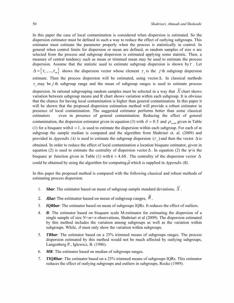
When there are outlying subgroups, the estimators given in methods 1 and 2 fail to estimate the process dispersion precisely. The above estimators including the proposed one must be multiplied by some correction factors to obtain the unbiased estimators under normality assumption. The correction factors are computed for different values of n using the algorithm given in Appendix(C) and presented in Table (2).

Table 2 correction factor for estimators defined by different methods

TIQRbarMR TRbar B IQRbarRbar Sbar *BB n

1.0068 1.0364 1.0051 0.641 0.8871 0.8865 1.2533 0.88 2

0.8275 0.6274 0.6228 0.641 0.7830 0.5907 1.1284 1.19 3

0.7820 0.5040 0.5009 0.641 0.7510 0.4857 1.0854 0.87 4

0.7874 0.4418 0.44 0.641 0.7517 0.4299 1.0638 0.87 ٥

0.81 0.4032 0.4 0.641 0.7766 0.3946 1.051 0.8 ٦

0.7827 0.3775 0.3764 0.641 0.7651 0.6398 1.0423 0.78 ٧

0.7728 0.358 0.3563 0.641 0.7592 0.3512 1.0363 0.76 ٨

0.7745 0.3425 0.3419 0.641 0.7537 0.3367 1.0318 0.74 ٩

0.7809 0.3300 0.3296 0.641 0.7608 0.3249 1.0281 0.73 10

0.7689 0.3203 0.3194 0.641 0.7524 0.3152 1.0252 0.72 11

0.7649 0.3119 0.3109 0.641 0.7520 0.3069 1.0229 0.72 12 *proposed method 3. ROBUSTNESS OF ESTIMATORS Three measures of robustness including Breakdown Point (BP), Influence Function (IF) and Maximum Bias (MB) are proposed by Maronna et al. (2006). While the breakdown point deals with larger proportion of outliers, the influence function considers only a small proportion. In addition, maximum bias measures the maximum bias of estimator as a function of the proportion of outliers. Among these measurements, the breakdown point is easier to use. Tatum (1997) defined

* /p mnBP = as the breakdown bound (BP*) of the control charts. In this definition p is the largest proportion of observations allowed to be outliers and still leaving the estimate bounded, m is the number of subgroups and n is the size of the sample. Maronna et al. (2006) defined a roughly similar definition for the breakdown point. It has been proven that the breakdown point of dispersion estimator using equation (3) is approximately 50%, Maronna et al. (2006). Thus, when the subgroup size is equal to 5, presence of 3 or more outlier observations in the subgroup can cause the estimate of subgroup dispersion to fall beyond any given bound. On the other hand, the breakdown point of location estimator obtained from equation (2) is approximately at 50%. As an example if the number of subgroups is equal to 30, the location estimator of dispersion vectorΔ remains bounded when the number of subgroups with inflated dispersion estimates is 14 or less. Thus, the breakdown point of the proposed method for estimating process dispersion depends on the sample size (n) and the number of subgroups (m).


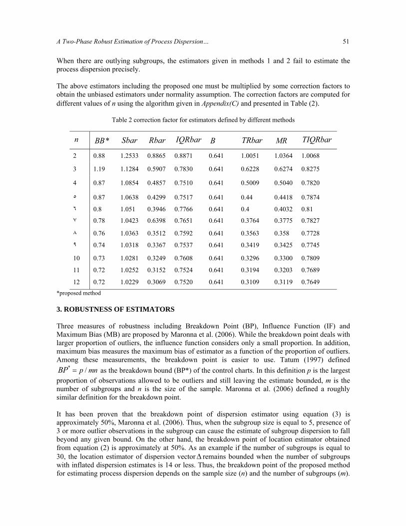
In the worst case it is shown that the breakdown bound for the proposed method is approximately 0.25 (BP* = ( / 2) ( / 2) 0.25m n mn× = ). The breakdown points for the other dispersion estimators are provided in Table 3.

Table 3 breakdown points for different dispersion estimators methods*

ESTIMATOR BB Sbar Rbar IQRbar B TRbar MR TIQRbar

BP 0.25 0 0

1 4 7.2 8 11.

if nm n

if nm n

⎧ ≤ ≤⎪⎪⎨⎪ ≤ ≤⎪⎩

0.5 1

4n

( 1)2

.

2.

for even

for odd

m

m

m

m nm

m n

⎧ −⎪⎪⎪⎨⎡ ⎤⎪⎢ ⎥⎪⎣ ⎦

⎪⎩

1

( ( 1) 1).

4

4

u

j

u jm nn

m

= +

=

+ −

⎡ ⎤⎢ ⎥⎣ ⎦⎡ ⎤⎢ ⎥⎣ ⎦

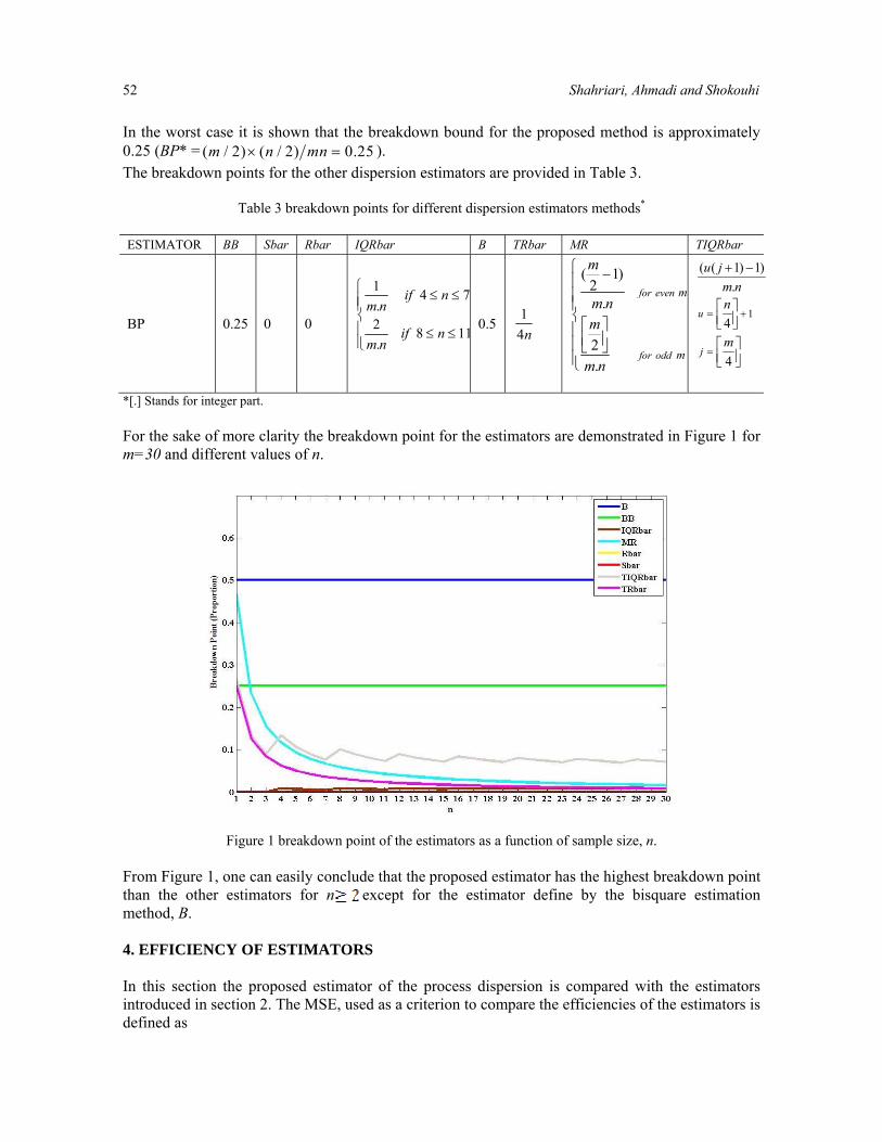
*[.] Stands for integer part. For the sake of more clarity the breakdown point for the estimators are demonstrated in Figure 1 for m=30 and different values of n.

Figure 1 breakdown point of the estimators as a function of sample size, n.

From Figure 1, one can easily conclude that the proposed estimator has the highest breakdown point than the other estimators for n except for the estimator define by the bisquare estimation method, B. 4. EFFICIENCY OF ESTIMATORS In this section the proposed estimator of the process dispersion is compared with the estimators introduced in section 2. The MSE, used as a criterion to compare the efficiencies of the estimators is defined as


( )∑=

−=k

iik

MSE1

2ˆ1 θθ (4)

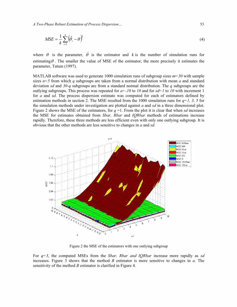
where θ is the parameter, θ is the estimator and k is the number of simulation runs for estimatingθ . The smaller the value of MSE of the estimator, the more precisely it estimates the parameter, Tatum (1997). MATLAB software was used to generate 1000 simulation runs of subgroup sizes m=30 with sample sizes n=5 from which q subgroups are taken from a normal distribution with mean a and standard deviation sd and 30-q subgroups are from a standard normal distribution. The q subgroups are the outlying subgroups. This process was repeated for a=-10 to 10 and for sd=1 to 10 with increment 1 for a and sd. The process dispersion estimate was computed for each of estimators defined by estimation methods in section 2. The MSE resulted from the 1000 simulation runs for q=1, 3, 5 for the simulation methods under investigation are plotted against a and sd in a three dimensional plot. Figure 2 shows the MSE of the estimators, for q =1. From the plot it is clear that when sd increases the MSE for estimates obtained from Sbar, Rbar and IQRbar methods of estimations increase rapidly. Therefore, these three methods are less efficient even with only one outlying subgroup. It is obvious that the other methods are less sensitive to changes in a and sd.

Figure 2 the MSE of the estimators with one outlying subgroup

For q=3, the computed MSEs from the Sbar, Rbar and IQRbar increase more rapidly as sd increases. Figure 3 shows that the method B estimator is more sensitive to changes in a. The sensitivity of the method B estimator is clarified in Figure 4.


Figure 3 the MSE of the estimators with three outlying subgroups

Figure 4 the MSE of the estimators with three outlying subgroups Results for q=5 are shown in Figure 5. This Figure shows that the methods Sbar, Rbar and IQRbar introduce less efficient estimators. Examination of Figure 6 reveals that the method B estimator is more sensitive to changes in a for small and moderate values of sds. The estimators from methods IQRbar and TIQRbar are more sensitive than proposed method for moderate and large values of sds.


Figure 5 the MSE of the estimators with five outlying subgroups

Figure 6 the MSE of the estimators with five outlying subgroups

5. CONCLUSIONS For the proposed estimation method the bisquare function was used twice to reduce the effects of both types of contaminations, specifically the local contamination. The breakdown point of the


proposed estimator is high among some estimators either classical or robust. So it is a more robust estimator compare to these estimators. The MSE as a measure of efficiency of an estimator is shown to be small for proposed estimator in compare to the MSE of the other estimators when local contamination exists. The sensitivity of the introduced estimator with respect to the changes in mean and standard deviation of the outlying subgroups, a and sd, respectively is roughly lower than the other estimators. So construction of any control chart based on this estimator could result in a more precise control limits in practical situations. The analyzer can rely on this control chart to control a process more comfortably. This may be verified by comparing the power of the test for this control chart and the others. REFERENCES [1] Huber P.J. (1981), Robust Statistics; John Wiley; New York.

[2] Langenberg P., Iglewicz B. (1986), Trimmed mean X and R charts; Journal of Quality Technology 18; 152-161.

[3] Maronna A.R. (2006), Robust statistics theory and methods; John Wiley; New York. [4] Montgomery D.C. (2005), Introduction to statistical quality control; 5th Edition, Wiley; New York. [5] Omar M. (2008), A simple robust control chart based on MAD; Journal of Mathematics and Statistics

4(2); 102-107. [6] Rocke D.M. (1989), Robust control charts; Technometrics 31;173–184.

[7] Rocke D.M. (1992), QX and QR charts: robust control charts; The Statistician 41; 97-104. [8] Shahriari H., Maddahi A., Shokouhi A.H. (2009), A robust dispersion control chart based on M-

estimate; Journal of Industrial and system engineering 2; 297-307. [9] Tatum L.G. (1997), Robust estimation of the process standard deviation for control charts;

Technometrics 39; 127–141. APPENDICES Appendix A

This section is due to Shahriari et al. (2009). The algorithm to compute M-estimate of scale is demonstrated in this appendix. Firstly, good start point should be calculated as initial estimation of location and dispersion. Sample median and normalized median absolute deviation (MADN) can be used in this case. MADN is calculated by

(| - ( ) |)0.6745

Med x Med xMADN = (A-1)

then weight function is defined as


ˆˆ

w W μσ−⎛ ⎞= ⎜ ⎟

⎝ ⎠x

(A-2)

where W is expression (A-3).

2( ) / 0( )

(0) 0x x if x

W xif x

ρ

ρ

≠=

′′ =

⎧⎨⎩

(A-3)

where ( )xρ is ρ -function. Then ˆnewσ can be estimated as

2

1

1ˆ ˆn

new old ii

wrn

σ σδ =

= ∑ (A-4)

where ˆ

ˆi

iold

xr μσ−

= . Moreover, μ is constant and σ is updated each iteration to estimate M-scale.

Also, both μ and σ are updated to calculate simultaneous M-estimation. Stop condition is when 1ˆ ˆ| / 1 |k kσ σ ε+ − < .” Appendix B

The algorithm to compute M-estimate of location is demonstrated in this appendix. Firstly, good start point should be calculated as initial estimation of location and dispersion. Sample median and normalized median absolute deviation (MADN) can be used in this case. MADN is calculated by

( ( ) )0.6745

Median X Median XMADN

−= (B-1)

then weight function for the ith observation at kth iteration is defined as

,

0

ˆ( )

ˆi k

k iXw w μσ−

= (B-2)

where 0ˆ MADNσ = , 0ˆ ( )Median Xμ = and W is expression (B-3).

( ) 0( )

( ) 0

x if xW X x

x if x

ψ

ψ

⎧ ≠⎪= ⎨⎪ ′ =⎩

(B-3)

where ( )xψ is ψ -function. Then let 1ˆkμ +


,1

1

,1

ˆ

n

k i ii

k n

k ii

w X

wμ =

+

=

=∑

∑ (B-4)

Note that 0σ is fixed and ˆkμ is updated each iteration to estimate M-estimate of location.

Stop condition is when 1 0ˆ ˆ ˆk kμ μ εσ+ − < , where ε is an arbitrary tolerance parameter. Appendix C

In the first step it was assumed some multiplier of the estimator is unbiased for parameter σ i.e.

σθ =)ˆ( nkE

where σ is the process dispersion and nk is a constant which depends on n. Then m subgroups of size n were generated from normal distribution with mean μ and standard deviation σ. Based on these data, an estimate of σ was computed called iθ . This procedure was repeated for 10000 times.

At the end of this step using

⎪⎭

⎪⎬⎫

⎪⎩

⎪⎨⎧∑=

10000ˆ10000

1iiθ

σ , an estimate of nk were obtained.

In the next step the null hypothesis 0

ˆ: ( )n

H Ekσθ = was tasted against 1

ˆ: ( )n

H Ekσθ ≠ where nk was

estimated in the previous step. For testing the hypothesis m subgroups of size n were generated from normal distribution with mean μ and standard deviation σ. By using these data, an estimate of σ was computed ( ˆ

jθ ). This procedure was repeated 1000 times. The random sample of size 1000, containing the values of ˆ

jθ was used to test the hypothesis. The null hypothesis was failed to reject at the significance level of 5%.

a two-phase robust estimation of process dispersion using ... · a two-phase robust estimation of...

Documents