a u uclassified 3**flfl**fl.f2 may amaximal flow … · should follow the main title, be separated...
TRANSCRIPT

A AMAXIMAL FLOW APPROACH TO DYNAMIC ROUTING IN COMMUNICATION NET--ETC(UJMAY G0 M4 JOOKOVSAT, A SEGALL NOOG IA-75-C-I18a3
U UCLASSIFIED LIDS-R-988 IA.3**flfl**fl.f2
LU-
III1 L 4 IIIILit VMICROCOP11 S 1
1111.25 llI 4 111.
MICROCOPY RESOLUTION TEST CHART

118001"l Supported AVARPA Co~twct NOGOI 4.75-C-i83OS Number 82933
ONR C0xtc N0001477XC-0332OSP Number 85552,LEVEIL
SC
A MAXIMAL FLOW APPROACH TO DYNAMICROUTING IN COMMUNICATION NETWORKS
Medo JodorkowdyAdrin Segll
Laboratory for Information and Decision Systems f' Pdn@bSiss mdl ld" IFormerly ,V,
Electronic Systems Laboratory
MASSACHUSETTS INSTITUTE OF TECHNOLOGY, CAMBRIDGE, MASSACHUSETTS 02139
8o6 3 03

%ECUPITY CLASSIFICATION OF THIS PAGE ("&Are Date Entered)
REPORT DOCUMENTATION PAGE BEFORE COMPLETIOGS. 'REPORT NUMBER 12. GbVT ACCESSION 3 RECIPIENT'S CATALOG NUMBER
A. ITE (ndSubite' * YP OF REPORT a PERIOD COVERED
SFlo App o tA Dynamc RoutingNUMECommunication Networks
. A WOR A UNIT NUMBERS
Laboratory for Information and Decision Systems Program Code No. 5T0LONR Identifying No. 049-383
Defense Advanced Research Projects Agency // MyU
14. MONITORING AGENCY NAME a ADDRESS(II dilfo~nmt from, Contronlnnh Offce) IS. 'SECURITY CLASS. (of t/te reor)
Office of Naval ResearchInformation Systems Program /JodUnolassified
ArlintonCde 43 VA 2217 /, / .'I...I I'S..
' ECLASSIFICATONIDOWNGRADINGs c E u L
C CFdriae 37 46#1HE5CDUL3
16. PISTR IUTION STATEMENT (oN tAMe Repo REt) "W UM-
Approved for public release; distribution unlimited.
m17. DISTRIUTION STATEMENT (of the ebefIac eettited gn BloNo .0 It dli.ent m Repo3t)
IS. SUPPLEMENTARY NOTES
. KEY WORDS (Continue on esereetdc ih necetes Agl identciy yblock n1mbe)
za. A fIRACT (Conilirme n ,ewereo side I! ncoeay lind Idontity by block numbe,)
This work presents a new approach for building the feedback solution forthe minimum delay dynamic message routing problem for single destinationnetworks.
The approach fully exploits the special structure of the constraint matriceobtained in the dynamic state space model suggested in previous works,
by transforming every linear program arising from the necessary conditions,into a maimal weighted flow problem.
Arigtn A 21
1D, DIS 173BU TIOS N O (of hs IS4o-660T
17 ITIUIN SEMNT (o2-f.Od60 SthRIT abAstrICacO OPtre InI BlAck 20,.. #1t dil tfrm eprt
7m
SECURITY CLASSIFICATION OF THIS PAGE (When Date Entered)
-- Taking advantage of several properties concerning the networks correspond-ing to the linear programming problems, all theorems regarding certainsimplifying characteristics of the feedback solution that apply in the caseof single-destination networks with all unity weightings in the costfunctional are reproved in a simplified and more straightforward manner.
A compact algorithm for the construction of the feedback solution ispresented, the algorithm being implementable on networks of reasonable size.
A method for obtaining all solutions of the linear programming problemsrequired by the algorithm, based on the application of linear programmingtechniques in networks is provided. The method is implemented by a computerprogram and several examples are run to test its applicability. IgorCi
In addition, a deep geometrical insight to every step of the lgorithmis given by deriving the explicit set of inequalities defining the problemconstraint figure in the state-velocity space.
The complexity of the problem is also analyzed, being exponential inthe number of the network nodes, thus giving an idea of the maximal networksize for which a full feedback solution can be obtained under the availablecomputational resources.
I Accesslon For
DI'C TAB.%ounc ed
Juitil ic-.tion
Bye.
TL AI I
SErCURITY CL.ASSIFlICATION Ofr
THIS PA09'llAMh DO" RA~tll /
INSTRUCTIONS FOR PREPARATION OF REPORT DOCUMENTATION PAGE
RESPONSIBILITY. The controlling DeD office will be responsible for completion of tho Report Documentation Page, DD Form 1473, inall technical reports prepared by or for DoD organizations.
QASS.IFICATION. Since this Report Documentation Page, DD Form 1473, is used in preparing announcements, bibliographies, and databanks, it should" be unclassified if possible. If a classification is required, identify the classified items on the page by the appropriatesymbol.
COMPLETION GUIDE
General. Make Blocks 1, 4. S, 6, 7. 11, 13, 15, and 16 agree with the corresponding information on the report cover. LeaveBlocks 2 and 3 blank.
Block I. Report Number. Enter the unique alphanumeric report number shown on the cover.
Block 2. Government Accession No. Leave Blank. This space is for use by the Defense Documentation Center.
Block 3. Recipient's Catalog Number. Leave blank. This space is for the use of the report recipient to assist in futureretrieval of th-ocument.
Bljck 4. Title and Subtitle. Enter the title in all capital letters exactly as it appears on the publication. Titles should beunclassified whenever possible. Write out the English equivalent for Greek letters and mathematical symbols in the title (see"Abstracting Scientific and Technical Reports of Defense-sponsored RDT/E,"AD-667 000). If the report has a subtitle, this subtitleshould follow the main title, be separated by a comma or semicolon if appropriate, and be initially capitalized. If a publication has atitle in a foreign language, translate the title into English and follow the English translation with the title in the original language.Make every effort to simplify the title before publication.
Block 5. Type of Report and Period Covered. Indicate here whether report is interim, final, etc., and, if applicable, inclusivedates of period covered, such as the life of a contract covered in a final contractor report.
Block 6. Performing Organization Report Number. Only numbers other than the official report number shown in Block 1, suchas series numbers for in-house reports or a contractor/grantee number assigned by hin, will be placed in this space. If no such numbersare used, leave this space blank,
Block 7. Author(s). Include corresponding information from the report cover. Give the name(s) of the author(s) in conventional* order (fore xample. John R. Doe or, if atithor prefers, J. Robert Doe). In addition, list the affiliation of an author if it differs from that
of the performing organization.
Block 8. Contract or Grant Number(s). For a contractor or grantee report, enter the complete contract or grant number(s) underwhich the work-reported was accomplished. Leave blank in in-house reports.
Block 9. Performing Organization Name and Address. For in-house reports enter the name and address, including office symbol,of the perforing activity. For contractor or grantee reports enter the name and address of the contractor or grantee who prepared thereport and identify the appropriate corporate division, school, laboratory, etc., of the author. List city, state, and ZIP Code.
Block 10. Program Element, Project. Task Area, and Work Unit Numbers. Enter here the numrber code from the applicableDepartment of Defense form, such as the DD Form 1498, "Research and Technology Work Unit Summary" or the DD Form 1634."Research and Development Planning Summary," which identifies the program element, project, task area, and work unit or equivalent
under which the work was authorized.
Btock 11. Controlling Office Name and Address. Enter the full, official name and address, including office symbol, of thecontrolling office. (Equates to funding/sponsoring agency. For definition see DoD Directive 5200.20. "Distribution Statements onTechn ical Documents. "')
Block 12. Report Date. Enter here the day, month, and year or month and year as shown on the cover.Block 13. Number of Pages. Enter the total number of pages.
Block 14 Monitoring Agency Name and Address (if different from Controlling Office). For use when the controlling or fundingoffice does not directly administer a project, contract, or grant, but delegates the administrative responsibility to another organization.
Blocks 15 & ISO. Security Classification of the Report: Declassification/Downgrading Schedule of the Report. Enter in ISthe highest classification of the report. If appropriate, enter in ISa the declassification/downgrading schedule of the report, using the
abbreviations for declessification/downgrading schedules listed in paragraph 4-207 of DoD 5200. I-R.
Block 16 Distribution Statement of the Report. Insert here the applicable distribution statement of the report from DoD
Directive 5200.20, "Distribution Statements on Technical Documents."
Block 17. Distribution Statement (of the abstract entered in Block 20, if different from the distribution statement of the report).
Insert here the applicable distribution statement of the abstract from DoD Directive 5200.20, "Distribution Statements on Technical Doc-
ument s. " I
Block 18. Supplementary Notes. Enter information not Included elsewhere but useful, such as: Prepared in cooperation with
Trans atonof (or by) . . . Presented at conference of. . . To be published in . . .
Block 19 Key Words. Select terms or short phrases that identify the principal subjects covered in the report, and are
sufficiently specific and precise to be used as index entries for cataloging, conforming to standard terminology. The DoD "Thesaurus
of Engineering and Scientific Tens" (TEST), AD-672 000, can be helpful.
Block 20, Abstract. The abstract should be a brief (not to exceed 200 words) factual summary of the most significant informa-tion contaih -inthe report. If possible, the abstract of a classified report should be unclassified and the abstract to an unclassified
report should consist of publicly- releasable information. If the report contains a significant bibliography or literature survey, mention
it here. For information on preparing abstracts see "Abstracting Scientific and Technical Reports of Defense-Sponsored RDT&E,"
AD-667 000. * ,

May, 1980 LIDS-R-988
A MAXIMAL PLOW APPROACH
TO DYNAMIC ROUTING IN COMMUNICATION NETWORKS
Mario Jodorkovsky and Adrian Segall
Department of Electrical EngineeringTechnion - Israel Institute of Technology
Haifa, Israel
I
The work of A. Segall was performed on a consulting agreement with theLaboratory for Information and Decision Systems at M.I.T., Cambridge,Mass., and was supported in part by the Advanced Research Project Agencyof the U.S. Department of Defense (monitored by ONR) under Contract No.N00014-75-C-1183, and in part by the Office of Naval Research underContract No. ONR/N00014-77-C-0532.

Contents
* I Abstract I
Glossary of Notations
SECTION 1 INTRODUCTION 2
SECTION 2: GENERAL DESCRIPTION OF THE ALGORITHM 13
A: Mathematical Statement of the Algorithm 13
B: All States Leave the Boundary 16
C: A Subset of States Leaves the Boundary 20
D: States Leaving the Boundary from ConstructedFeedback Control Regions 27
SECTION 3: THEORETICAL RESULTS 30
A: The Structure of the y-Constraint-Figure inthe Positive Orthant 6f the y-Space 30
B: Special Properties of the Feedback Solution for4Single Destination Networks with all Unity
Weightings in the Cost Functional 38
SECTION 4: THE ALGORITHM 58
A: Statement of the Algorithm 58
B: The Method for Finding all Solutions to theLinear Programming Problems 65
C: Example of Feedback Solution to the DynamicRouting Problem of a Single Destination Networkwith all Unity Weightings in the Cost Functional 73
SECTION 5: CONCLUSIONS 94
Appendix A: Basic Concepts of Graph Theory, Maximal Flow andLinear Programming in Networks 96
Appendix B: Computer Programs 104
References: 111
U. .----------

i Abstract
This work presents a new approach for building the feedback solution
for the minimum delay dynamic message routing problem for single destination
networks.
The approach fully exploits the special structure of the constraint
matrices obtained in the dynamic state space model suggested in previous works,
by transforming every linear program arising from the necessary conditions,
into a maximal weighted flow problem.
Taking advantage of several properties concerning the networks cor-
responding to the linear programming problems, all theorems regarding certain
simplifying characteristics of the feedback solution that apply in the case
of single-destination networks with all unity weightings in the cost functional
are reproved in a simplified and more straightforward manner.
*A compact algorithm for the construction of the feedback solution is
presented, the algorithm being implementable on networks of reasonable size.
A method for obtaining all solutions of the linear programming prob-
lems required by the algorithm, based on the application of linear programming
techniques in networks is provided. The method is implemented by a computer
*program and several examples are run to test its applicability.
In addition, a deep geometrical insight to every step of the algor-
ithm is given by deriving the explicit set of inequalities defining the prob-
lem constraint figure in the state-velocity space.
The complexity of the problem is also analyzed, being exponential in
the number of the network nodes, thus giving an idea of the maximal network
size for which a full feedback solution can be obtained under the available
- computational resources.

Glossary of Notations
Notation Definition
N - set of network nodes not including the destination node
L - set of network links
(i,k) - directed link from node i to node k
c ik - capacity of link (i,k)
x - vector of state variables
y - vector of velocity of state variables (-x)
u - vector of control variables
A - vector of costates
U - constraint figure in u-space
V - constraint figure in y-space
Ip - set of states travelling on interior arcs on [t ptp+ )
"B - set of states travelling on boundary arcs on [t ,t )P p p+1
L - set of states leaving the boundary at t backwards in timep p
R - feedback control region constructed from optimal traject-p
ories on the segment [t ptp 1 )
Y p - set of operating points on [t p,t p+)
(XJ) - a minimal cut of the network
b. - demand for flow in node i1
b S - supply of flow to the network
a - cardinality of Ip P
p - cardinality of Lp P
H(T) - the Hamiltonian at T
Co(.) - Convex Hull
E(i) - Collection of nodes k such that (i,k) c L
I(i) - Collection of nodes Z such that (1,i) c L
-2-
Section 1
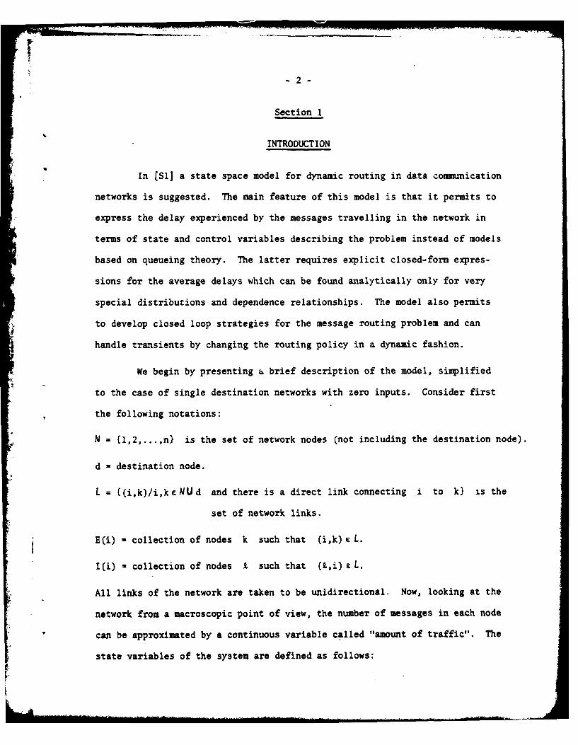
INTRODUCTION
In [S1] a state space model for dynamic routing in data communication
networks is suggested. The main feature of this model is that it permits to
express the delay experienced by the messages travelling in the network in
terms of state and control variables describing the problem instead of models
based on queueing theory. The latter requires explicit closed-form expres-
sions for the average delays which can be found analytically only for very
special distributions and dependence relationships. The model also permits
to develop closed loop strategies for the message routing problem and can
handle transients by changing the routing policy in a dynamic fashion.
We begin by presenting a brief description of the model, simplified
to the case of single destination networks with zero inputs. Consider first
the following notations:
N = {1,2,...,n} is the set of network nodes (not including the destination node).
d = destination node.
L = {(i,k)/i,ke NUd and there is a direct link connecting i to kJ is the
set of network links.
E(i) - collection of nodes k such that (i,k)E L.
I(i) - collection of nodes X such that (2,i) e L.
All links of the network are taken to be unidirectional. Now, looking at the
network from a macroscopic point of view, the number of messages in each node
can be approximated by a continuous variable called "amount of traffic". The
state variables of the system are defined as follows:

-3-
x (t) amount of traffic at node i, at time t, where i N.
The control variables are defined as:
Uik(t) amount of traffic on link (ik) at time t where (i,k) e L.
The dynamics of the system are given by the equations describing the rate of
change of the contents of each node, namely:
i - UiA(t) + U zi(t) (1.1)ke-E~i) teI(i)
The constraints are:
x (t) > o (l.2a)i
and
U: 0 < U. (t) < c (l.2b)in - ik
where
ck capacity of link (i,k) in units of traffic/unit time, where
(i,k) e L.
The cost functional is taken to be the total delay experienced by the
messages travelling in the network, starting at a given time t and ending at
a time tf when the network is emptied, i e x (t = 0, V i e N. The ex-
pression for the above quantity is
tJ f x i(t)]dt • [1.3)
I tot0
From now on, the various variables of the model will be represented in vector
form as follows: Denoting by x and u the respective concatenations of
state variables and controls, to every differential constraint in (1.1) cor-
responds a vector bi such that:
-4-
= b.u~1 -1-
where the vectors b. are the rows of the incidence matrix B of the network.
Now we express the linear optimal control problem with linear state
and control variable inequality constraints representing the data communication
network closed loop dynamic routing problem as stated in [Sl]:
Find the set of controls u as a function of time and state,
( 4 u(t,x) , t '[toptf ] I
that brings a given initial condition x(t) = x to the final condition
x(tf) = 0 and minimizes the cost functional (1.3) subject to the dynamics (1.1)
and to the state and control variable inequality constraints (1.2).
It is well know that in most optimal control problems it is quite
difficult to obtain feedback solutions. In our case however, owing to the
linearity of the problem, we can cover the entire state space with optimal
controls by solving just a comprehensive set of linear programs. In [SI]
an approach is suggested, by way of a simple example for constructing the
feedback solution. In [M], (M2] and (M3] this approach is elaborated upon
by developing the so called Constructive Dynamic Programming Algorithm for
the construction of the feedback solution. We proceed now with a brief pre-
sentation of the results obtained in the above works and the conceptual
lines of the Constructive Dynamic Programming Algorithm in order to provide
the reader with basic notions for the understanding of the present report.
We begin by presenting the necessary and sufficient conditions of optimality:
Theorem 1.1: (See [Ml, pp. 53-63] or [M2, pp. 13-20]).
Let the scalar functional h be defined as follows:
h( (t),XCt)) i X T (tlt) X T (t)Bu~t).

A necessary and sufficient condition for the control law u*(') C U to be
optimal for problem (1.1) - (1.3) is that it minimizes h pointwise in time,
namely:
SA(t)Bu*(t) < XT(t)Bu(t) (1.4)
V u(t) eU, t C [to ,t f]
The costate X(t) is possibly a discontinuous function which satisfies the
following differential equations:
-dXi(t) = dt+dui.(t), V ieN t E[totf] (1.5)1 1 .
where componentwise dP . (t) satisfies the complementary slackness conditions:-- 1
xi (t)dui (t) = 0 t E [tot f ]
* (1.6)dui(t) < 0 ieN
The terminal boundary condition for the costate differential equation is
A(tf) = 0 free , (1.7)
and the transversality condition is
T (tf )x(tf) = 0 (1.8)
Finally, the function h is everywhere continuous, i.e.:
h(u(t-),(t)) = h(u(t ),X(t)), V t e (tot f]oIf03 Theorem 1.1
From inequality (1.4) of the necessary and sufficient conditions we
see that th. optimal control function u*(.) is given at every time
t [ttf] by the solution of the linear program
u*Q(r) = ARGMIN(kT (r)Bu.(T)] (1.9)u(r)cU

-6
From (1.9), and owing to the structure of the incidence matrix B, it follows
that there always exists an optimal solution for which the controls are piece-
wise constant in time. Moreover, since the equations governing the dynamics
of the system are linear, the corresponding state trajectories have piecewise
constant slopes. From the nature of the controls follows that every optimal
trajectory may be characterized by a finite number of parameters. These para-
meters are:
u(x) {u u , l...,AU f-l
and
T(x) {to t1 ... tf}
where U(x) is the sequence of optimal controls, T(x) is its associated
control switch time sequence, and the element u is the optimal control on-p
, t [tpptp+l], c[,,.. -]
Moreover, every segment of an optimal trajectory, say the segment
[tp t,] is characterized by the following parameters:
B = {xi/xi(T) = 0 'T (t p,t p )1
andI {xi/xi (T) > 0 T C[,t p+)}
that is, B and I are the sets of states travelling on boundary arcs andp p
interior arcs respectively on [t ,t ). Now, the main fact following fromp p+l
the nature of the optimal trajectories is that the state space can be divided
into regions, each one being a convex polyhedral cone, when to every point of
a specific region corresponds an identical set of optimal controls. This is
exactly the reason that makes the construction of a feedback solution possible.
The above regions are referred to as "feedback control regions" and are de-
noted by R.
The problem is then to construct these feedback control regions, there-
by specifying the optimal control for every point of the state space. Now,
-7
considering the special geometric characterization of the feedback space, and
thinking in the spirit of dynamic programming, let us look at the optimal
trajectories backwards in time, beginning at tf. We will then see a sequence
of states leaving the boundary (perhaps two or more at a time) and varying
with constant slopes. Now, in (M2] it is proven that if any state variable,
say xi, is strictly positive on the last time interval (tf-1 1tf] of an
optimal trajectory, then Xi(tf) = 0. Moreover, by (1.6) we know that for
this state we have dui.('r) = 0 VT [tf-1 1tf] so that by (1.5) we obtain
X• .() -1 V T C [tf 1 ,tf].
Now suppose we had decided to check if there exist optimal traject-
ories in the state space with a specified set of states If. I travelling on
interior arcs in the last interval and with the remaining states travelling
on boundary arcs. Since we know the costates corresponding to the states in
If-i (by the above arguments) and using (1.9), these trajectories may be
found by solving the following linear program:
Find all:
* ARGMIN ) ARGMIN X (-)biu
-u. tU t.I If-1 ucU x CIf-i
s.t. (1.10)
xi <0 X If-l
j Z0 Vx i e f.
The linear program (1.10) is called the constrained optimization prob-
lem and its solutions are trajectories only provided that there exist values
A Vxj c Bf.1 that satisfy the necessary conditions (l.S) - (1.6). Moreover,
the solutions of (1.10) provide optimal directions x Ct Ix in the
state space, defining the convex polyhedral cone corresponding to the feedback

-8-
control region characterized by the set of controls that solves (1.10). Now,
solving such a linear program for every possible combination of state vari-
ables leaving the boundary (backwards in time) at tf, we obtain feedback
control regions containing all points from which the origin can be reached
while maintaining sets If away from the boundary for all t < t In fact
the linear program (1.10) must be solved parametrically in time until the con-
trol changes. A change in the control defines a hyperplane passing through
the origin called "breakwall". By solving (1.10) until the cont-rol does not
break any more, we obtain a convex polyhedral cone divided by breakwalls into
a finite number of regions. Each region is characterized by a specific control
set and is referred to as "break feedback control region". The last region
constructed when solving (1.10), (i.e. when there are no more breaks in the
control) is called "non-break feedback control region".
In order to continue with the description of the algorithm, let us
introduce the following definition:
L = (xi/x i eB and x. is designated to leave the boundary
backward in time at t •p
Now, in order to cover the whole state space with optimal controls,
we must take every feedback control region already constructed and allow every
possible combination of states still travelling on the boundary to leave it,
backward in time. In general, this step is performed as follows: Denoting
by R the feedback control region constructed from the optimal trajectoriesp
on the segment [tpItp.1), pick a set of states of Bp, say L and parti-
tion Rp into "subregions" with respect to L p. The concept "subregion"
will be explained later. In order to let L leave the boundary at a certainp,
time t (called boundary junction time), we must find the costate values
i (tp) ixi eLp that allow the departure of the states in Lp from the

-9-
boundary while still being optimal. The above costate values are referred to
as "leave-the-boundary costate values". In geometrical terms the above co-
state values are found as follows:
By defining
y =-x -Bu
and
t C . n/ueU)
we can transform the linear program (1.9) into the f6llowing linear program
with decision vector y(r):
Y*(T) - ARGMAX T (T)Y(T) , (1.11)- y('r cV"
so that at t we can consider the hyperplane given by Z(t) = .J(t p)y
(called the Hamiltonian) tangent to V (called the y-constraint figure) that
provides points of tangency Y (called operational points) that are in factp
thq optimal directions in the state space defining the feedback control
region R p. Now in order to find the leave-the-boundary costates for L ,
we rotate the Hamiltonian around Y until we touch a surface of tangency? pof Y called L p-positive face, having at least one point with
> 0 Y xi Lp
The new orientation of the Hamiltonian gives the desired leave-the-boundary
costates and now we solve a linear program of the form:
Find all:
u* ARGNIN ir)=i ARGMIN X i (')biuucU x. I xiCIp-i
z.p-lI.P
s.t.i. 0 p-xi C Ip 1 I p ULp (1.12)
i "0 V xi C Bp I Bp /Lp
T C (tp,tp p

- 10 -
where (1.12) is again solved parametrically in time until the control breaks.
A subregion of R is the set of all points which, when taken as the
point of departure of L , result in a common set of optimal controls.~p
Clearly, such a partitioning of R may exist since to two distinct points in~p
R correspond different leave-the-boundary costates. In geometrical terms,
we could see the Hamiltonian rotating according to the change in the costates
when the states are travelling in R . When allowing Lp to leave thepp
boundary from distinct points of Rp, the Hamiltonian could meet different
L -positive faces, therefore giving different leave-the-boundary costate values.
p
The steps described for the construction of feedback control regions
form the so-called Constructive Dynamic Programming Algorithm as stated in
[Ml], [M2] and [M3]. Several features make the algorithm to be a conceptual
one rather than an implementable one. Among them, breaks in the optimal con-
trois, the existence of the subregions just pointed out, non-uniqueness of the
leave-the-boundary costates, and non-global optimality of certain sequences,
in addition to computational complexities associated with the algorithm, for
instance the problem of finding all solutions to linear programs. However,
it turns out that when dealing with single destination networks, and when no
priorities are assigned to the nodes (that is the cost functional has unity
weightings), many simplifications are attained, leading to a compact and imple-
mentable algorithm at least for moderate size networks.
In the present paper, we deal with the construction of the feedback
solution to the minimum delay dynamic message routing problem for single
destination networks, with zero inputs and when the cost functional has unity
weightings. The approach used to tackle the problem is based on the trans-
= - 11 -
formation of every linear program into a maximal weighted flow problem. The
transformation permits not only to develop a compact algorithm for obtaining
the feedback solution, but also to prove in a straightforward manner all the
simplifying features characterizing the feedback space, to develop a suitable
method for finding all the solutions to the linear programming problems and
to obtain explicitly the constraint figure in the state velocity space for
the geometrical understanding of the algorithm. The approach also permits
to gain insight into the complexity of the problem, thus providing the
essential information needed to estimate the maximal size of the networks for
which a complete feedback solution can be obtained under the available compu-
* tational resources.
One of the most interesting features of the algorithm presented here
is that although the efficiency of the method for obtaining all optimal solu-
tions to the linear programs is reduced by the high degeneracy of the problems
at hand, this is compensated by the fact that the higher the degree of
degeneracy, the lower is the number of linear programs that have to be solved.
Moreover, the algorithm requires to check all possible sequences of states
leaving the boundary backward in time or, in other words, all the possible
trajectories in the state space to insure the complete covering of the state
space. Again the higher the degree of degeneracy, the lower the number of
such sequences that have to be actually checked, thus obtaining a further
reduction in the complexity of the algorithm
The organization of the paper is as follows:
In Section 2, a general description of the algorithm is presented and
the transformation of the linear programs into maximal weighted flow problems
is introduced. Section 3 is devoted to the theoretical results obtained,
namely, the structure of the y-constraint figure and the proofs regarding all

- 12-
simplifying features of the feedback solution that apply in the case of single
destination networks.
In Section 4 the algorithm is presented in a compact form, the method
for obtaining all solutions to the linear programs is described and an example
of the construction of the feedback solution is given.
Finally, in Section 5 a brief discussion about the contributions of
this work is carried out and topics for further research in the area are
suggested.
0
.1
l,.

- 13 -
Section 2
GENERAL DESCRIPTION OF THE ALGORITHM
We begin with a brief preview of this section. In part A we present
a simplified mathematical description of the Constructive Dynamic Programming
Algorithm for building the feedback solution for the minimum delay dynamic
message routing problem for single destination networks with all unity weight-
ings in the cost functional. The algorithm consists of two steps. In the
first step, we construct feedback control regions resulting from the states
leaving the boundary at the final time (backward in time). The method to con-
struct these regions is depicted in parts B and C of this section. In the
second step, the rest of the state space is filled with optimal controls by
constructing the feedback control regions resulting from states leaving the
boundary, starting from already constructed regions. Part D of this section
deals with the construction of the above regions.
A. Mathematical Statement of the Algorithm
In [M2], the following properties associated with the Constructive
Dynamic Programming Algorithm are mentioned:
(a) Non-global optimality of certain sequences of state variables leaving
the boundary backwards in time.
(b) Non-uniqueness of leave-the-boundary costates.
(c) Subregions.
(d) Return of state variables to boundary backwards in time.
(e) Breaks in the optimal control between boundary junction times.

- 14 -
In [M3], a discussion of the above properties is presented in geo-
metrical terms. These problems complicate the formulation of a computational
scheme to implement the algorithm. However, as we will prove in Section 3 of
this paper, it turns out that these problems do not apply in the case of
single destination networks with all unity weightings in the cost functional,
thus permitting the following simplified statement of the algorithm:
Step 1: Solve the following series of linear programming problems:
Find all
* =ARG14IN ~ .=ARGMIN b buucU xiCLf 1 ueu xi eLf-
5.t.
x' < 0 Vx L (2.1)
--=o VxcB-
j f-i
for all Lf C {xi/iCN}
when Nl denotes the set of nodes not including the destination.
Step 2: For all feedback control regions Rp
(a) Calculate the leave-the-boundary costate values Xi (tp ) for all
x. c B, t being an arbitrary boundary junction time.1p p
(b) Solve the following series of linear programming problems:
Find all:
- ARGMIN x ii (t = ARGMIN X i(t p)biuutu x.rI 1 utU x.sI 1 P -,- 1 p-I - 1 -i
s.t.
<0 Vxi Ip-1 (2.2)
x ._0 VxiXp. 1
for all L -B .P P

is -
As we said before, in the first step, feedback control regions result-
ing from the states leaving the boundary at tfV are constructed. Note that
in problem (2.1), the cost function has unity weightings. The reason is that
by Corollary 2 in (M2], Ai(tf) = 0 Vx eLf, and by the necessary and suffici-i fi f
ent conditions for optimality (see [M2, pp. 13-17]), A.() = -1 Vxi eL
Moreover, since there are no breaks between boundary junction times, the co-
states corresponding to states in Lf are equal for all r £ (--,t ) so that
at every time in this interval the cost function is the same after normaliza-
tion. From this fact follows that at every time in (--,tf) we obtain the
same set of optimal solutions to problem (2.1), so that the time plays no role
here. Notice also, that since each set of state variables leaving the boundary
corresponds to a globally optimal solution, every solution to (2.1) gives an
optimal trajectory.
In the second step, feedback control regions resulting from states
leaving the boundary from previously constructed regions are built. Since
there is only one subregion per region, it follows that from every point of
a given feedback control region, states leave the boundary with the same con-
trol set and therefore boundary junction times may be chosen arbitrarily. The
above reasoning together with the fact that the leave-the-boundary costates
are unique for a given boundary junction time, and with the fact that no state
variable is ever required by optimality to increase forward in time, justify
the simplifications obtained in the statement of the algorithm.
The first step is carried out as follows: First, the linear program
corresponding to the leave-the-boundary of all states is solved. Second, the
linear programs corresponding to (n-1) states leaving the boundary are solved
(when n is the number of nodes in the network not including the destination
node), and so on. As it will be shown later, this. way of solving the first

- 16 -
step enables in genelal a considerable reduction in the number of linear pro-
grams that have to be solved. Moreover, it will also be shown later that in
fact the second step does not require solving any linear programs, thus greatly
reducing the complexity of the algorithm.
B. All States Leave the Boundary
According to (2.1), the linear programming problem we have to solve for
this case is:
Find all:
u* = ARGMIN x *. = ARGMIN I b.u , (2.3)udU ieN 1 ueU ieN
S.t.
x. < 0 YieN , (2.3a)1 -
0 <ujk C jkU = (2.3b)
Y (j,k) e L
Adding slack variables yi > 0 to the differential constraints (2.3a), prob-
lem (2.3) is transformed into:
Find all:
u* = ARGMIN E b.u = ARGMAX Z yi , (2.4)ucL ieN " ucU icN
S.t. .
Xi+Yi . 0Y i eN ,(2.4a)
Yi >0
0 < ujk <1cjk
U- (2.4b)
N o ,k) t L
Notice that in terms of the variable "y", the minimization problem (2.3) is
- 17 -
transformed into the maximization problem (2.4).
Suppose we are interested in finding only one solution to problem (2.4).
In order to do this, we transform the linear program (2.4) into the following
Maximal Flow Problem:
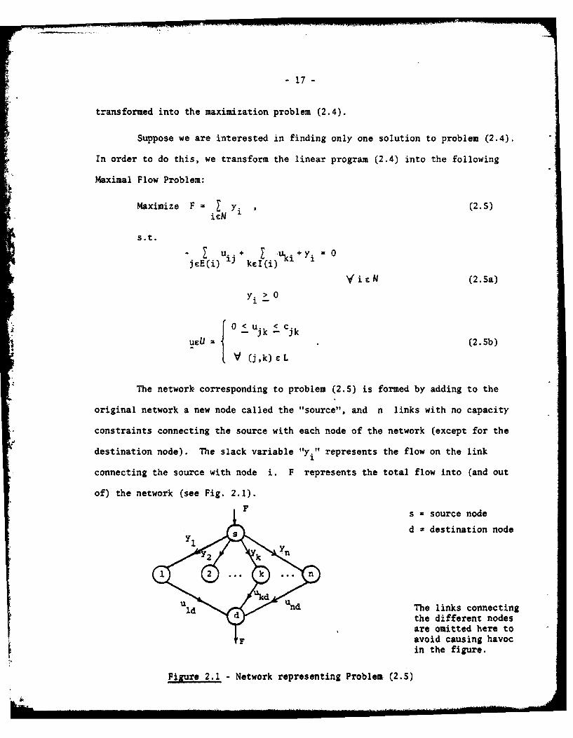
Maximize P = yi (2.5)ieN
S.t.- u..+ I iYi
j E(i) k. kI (i),
Si • N (2.5a)
Yi > 0
0 < U Cjk
uEU (2.5b)
V (j,k) e L
The network corresponding to problem (2.5) is formed by adding to the
original network a new node called the "source", and n links with no capacity
constraints connecting the source with each node of the network (except for the
destination node). The slack variable "yi" represents the flow on the link
connecting the source with node i. F represents the total flow into (and out
of) the network (see Fig. 2.1).
F s - source node
Y 12kd - destination node
ind The links connectingthe different nodesare omitted here toavoid causing havocin the figure.
Figure 2.1 - Network representing Problem (2.5)

- 18 -
The transformation of the- linear program into a Maximal Flow Problem
is the fundamental step required for the proofs of the theorems regarding the
simplifying properties of the feedback solution. In Appendix A, we give basic
concepts of graph theory that we use in the development of the algorithm and
in the proofs of the theorems.
Now we continue with the solutions of problem (2.5). Our aim is to
find one solution to problem (2.5) by means of the Maximal Flow Algorithm and
then, without changing the flow achieved in the first optimal solution, to per-
form all possible pivots on the network in order to find all the remaining
optimal solutions of problem (2.5). Notice that since we are seeking extremal
optimal solutions, we require that the first one will be an "extended basic
optimal solution", (see Appendix A). In this way every solution obtained by
pivoting will also be an extended basic optimal solution, thus representing an
extremal point in the optimization space. It turns out that finding a first
"extended basic optimal solution" to problem (2.5) is trivial. From the fact
that the links corresponding to the "y" variables do not have capacity con-
straints follows that there exists only one minimal cut in the network (denoted
by (X,X)), and it is composed by all the links connecting the nodes with the
destination; thus:
K = (s,l,2, .. ..nl
= {d)
Then we choose as the first optimal solution the following flows:
Cid i C l(d)
yi =
0 otherwise
(2.6)
uid c id YieI(d)
u * uki 0 j cE(i), kcI(i)
/icN

- 19 -
and
F = Ci (2. 6a)ii (d)id
Clearly, (2.6) is an "extended basic solution" if the variables yi
are declared basic and the remaining variables are declared non-basic. Notice
that if there is no direct connection between a node, say node i, and the
destination node, then the variable yi is basic with value zero. Now, since4i
networks have generally many nodes not connected'directly with the destination
we are dealing here with linear programming problems of a high degree of
degeneracy. The degeneracy problem lowers the efficiency of linear program-
ming methods, however in our case, the higher the degree of degeneracy, the
lower is the number of linear programs we have to solve. This subject will
be discussed in Part C of this section.
Recall that after finding the first "extended optimal basic solution"
we are interested in maintaining the achieved flow to assure that every solu-
tion obtained by pivoting operations on the network will be optimal. But
maintaining maximal flow in the network implies that at every solution the
flow on the minimal cuts will be constant and maximal; thus, before pivot-
ing we can reduce the number of variables of the problem by transforming the
network to the one depicted in Figure 2.2:F bF~s
Y2= 2 Yblb
-b -b -b -b
2 k
Figure 2.2 - Network configuration before the pivoting operation.

-20-
In Figure 2.2, b. accounts for the "demand" of flow in node i, and1
bs is the "supply" of flow to the network where:s
b. = i I(d) N
1 I0 otherwise
(2.7)b c Cids ieI(d)
Clearly, the reduction in the number of links facilitates the work of finding
all optimal solutions. After the reduction, the remaining optimal solutions
are found by means of the algorithm we present in Section 4.
C. A Subset of States Leaves the Boundary
In this case, we let a subset L C.{x./ic N}, such that L $ {xi/ic k)f 1f 1
to leave the boundary at tf, while all other states B remain on thef-i
boundary. By (2.1), the linear program to be solved is:
Find all:
* ARGMIN Z x. = ARGMIN b.u (2.8)ueU xicL 1 ueU x -eL'
S.t.< 0 V xi Lf
(2.8a)
--0 V x CBf-l
Transforming (2.8) into a Maximal Flow Problem, we have:
Maximize F Yi (2.9)
S.t.

- 21 -
- u..+ ) uki+Yi = 0 Lf
[u.. 7 i--o x i CBf Ir jcE(i) 'j kel(i)
(2.9a)
Yi > 0 x.E L f
0 Ju.k < cjk
U=
V(j k)eL
The network corresponding to problem (2.9) is formed by adding a new
node called the "source" to the original network, as in Part B of this section.
The difference here is that we add links without capacity constraints connect-
ing the source only with those nodes that correspond to state variables of Lf.
Nodes corresponding to state variables in B will be not connected with the
f-i
source. For example, Figure 2.3 shows a network with five nodes corresponding
to the case of two states leaving the boundary:
• F
Figure 2.3 - Example of network when only some states leave the boundary.
Our aim is, as in Part A, to find a first "extended basic optimal solu-
tion" to problem (2.9) and then by pivoting to find the remaining solutions.
But here we cannot obtain the first optimal solution by inspection since it is

- 22 -
not trivial to localize a minimal cut in the network. Moreover, we can obtain
an optimal solution by applying the Maximal Flow Algorithm to the network, but
this solution may not necessarily be an extended basic one. In order to over-
come this difficulty we present now two theorems and a corollary that will
assist us in developing a method to solve the problem when only some states
leave the boundary. In addition these results will show that in general there
are many combinations of state variables leaving the boundary for which it is
not necessary to solve a linear programming problem.
Theorem 2.1
Consider the following two linear programming (or Maximal Flow) problems:
Problem I
Maximize F- y.if
x: xi E Li
s.t.
- u.. uki.y.o YxiELjeE(i) 'J kcI(i)
jeECi) 3 kEI(i) 1 f-I
Y > 0 V x. c L'
ueU
Problem II
Maximize F2 = YiXi£Lf
- + y i =o V i fjEc(i) 13 kpI(i)
uj- uki =0 Vx B f_jcE(i) 3 kel(i) 1 f-I
Yi > 0 q4x.cLf
UCUwhere L' CLiaxi/ieN )

- 23 -
If in problem I exists a basic optimal solution with (y. = 0,
Vx. e L/Lf}, then all the basic optimal solutions of II are basic optimal
solutions of I. Moreover, for the networks representing the above problems,
all minimal cuts of II are minimal cuts of I.
Proof
Take the solution of I with {yj 0, Yx e L/LfI. This solution
satisfies the constraints of II and clearly Max F1 = Max F2. Now take allu£U ueU
basic optimal solutions of II and add new variables (y, .O, V x, e L'/L }f f
as non-basic ones with value zero. Clearly all these solutions satisfy the
constraints of I. Moreover, since Max F1 = Max F2' and .the new variables
were added as non-basic ones, the solutions are also basic optimal solutions
of I.
For the corresponding networks, take now all solutions of I with
ly. = , x. £ L'/Lf . Removing the links corresponding to fy./x. e LLf}3 33
will give the network configuration of II, and hence all the minimal cuts of
II are minimal-cuts of I.
0 Theorem 2.1.
Theorem 2.2
With the notation of theorem 2.1, suppose that there is no set L'~f
such that LfC Lj, and that all basic optimal solutions for Lf are also
basic optimal solutions for L'. Then a minimal cut for Lf is (X,X), whereff
X {CiN)U {s}/x i eLf.
Proof
The proof will be carried out by contradiction. Clearly every node
{i/x i c Lf} belongs to X since there are no'upper bounds on the variables
y.. Now, suppose that there exists a minimal cut (X',R') such thati
X' - X(JJ where x .L Then we can add to the network of problem II a new

- 24 -
non-basic variable yj > 0 with value zero (i.e., a link connecting the
source with node j with zero flow). By Theorem,2.1, all basic optimal
solutions of II are also basic optimal solutions of I, where L, = Lf Uxf f
in contradiction to the assumption that there exists no such set.
03 Theorem 2.2
Corollary 2.1
Under the assumptions of Theorem 2.2, when maximal flow is achieved,
all links:
{(ik) eL/x i eLf , xk L f )
have a flow equal to c ik and all links:
{(j,i) s L/xi eLf, x. Lf}
have flow with value zero. (Follows from Theorem 2.2 and the Max-Flow-Min-Cut
Theorem).
[ Corollary 2.1
Now we are able to present a method for solving problem (2.8). Re-
call that step 1 of the algorithm calls for solving a series of linear pro-
grams: First the linear program corresponding to all states leaving the
boundary, then those corresponding to all combinations of (n-l) statesleaving the boundary, etc. In other words, if L and L2 are two sets of
Lf an fartwseso
states leaving the boundary corresponding to two successive substeps of
2 1step , then cardinality L f < cardinality Lf. Now suppose that the current
substep of step 1 corresponds to the set of states Lf. If in an earlier
substep (say, corresponding to the set Lj) we obtained a basic optimal solu-
tion with fy a 0, V x£ Lj/Lfj and LfC L', then by Theorem 2.1 all
optimal solutions of the current substep (Lf)* are included in the set of
optimal solutions of the earlier substep (LI). Therefore we do not need to
solve the linear program corresponding to the current substep. In algorithmic

- - 25 -
terms, there are two ways for checking the existence of such a set L
1. To search all solutions obtained in earlier substeps corresponding
to sets L' where Lf C Lj, while looking for a solution with
{yj = 0 Vx. e LVLf}.
2. To find the Maximal Flow corresponding to the current substep (Lf)
and then to look for earlier substeps L such that LfC Li with
the same value of Maximal Flow.
Method (2) follows from the proof of Theorem 2.1.
Suppose now that there is no set L' such that LfC L' and such
that the problem corresponding to Li has an optimal solution with
{y. = 0 Vx.e L~,I}. In this case we apply to the network corresponding to
Lf. the Maximal Flow Algorithm. According to Corollary 2.1, when maximal
flow is achieved, the network can be partitioned into two subnetworks as
shown in Figure 2.4:
xk E Bf-1X ik ik.
s0
xi C Lf cut
Figure 2.4 - The two subnetworks separated by a minimal cut.
Recall that since we are building a feedback control region, we are
searching for all extremal values of (yi/xi c Lf} and the corresponding
controls (ujk/(j,k) e L}. But we notice that only pivots on the subnetwork
corresponding to X will lead to new extremal values of (y I/xi e Lf, so

-26-
that in order to obtain all optimal solutions to the problem corresponding
to L we concentrate on the reduced network depicted in Figure 2.S:
b
Xi C Lf
Figure 2.5 - Network configuration before the pivoting operation.
In Figure 2.5 we define:
cid + c . . i e I(d) (I I(k/xk c Bf_ 1 )jcet(i) 1J
x Lf
b. - .c.. V iOl(d) and icl(k/xkeBflI) (2.10)" i jCE (i) i
xj Lf
c id VieI(d) and i4I(k/xkcBf 1 )
0 otherwise
bs bi. (2.lOa)
For the first basic optimal solution we take
Yi = bi V xi e Lf
(2.11)
uij S 0 V xieLf , j cE(i)f {i/x i e L f }
By pivoting on the network of Figure 2.5, we obtain all the required
optimal solutions, when for each solution the flow values on the links in
are equal to those achieved when applying the Maximal Flow Algorithm.
-27-
Notice that at every substep of step I a further reduction of the net-
work is obtained. Moreover, from considerations of Theorem 2.1, there might be
many substeps for which there is no need to solve a linear program.
D. States Leaving the Boundary from Constructed Feedback Control Regions
We deal here with step 2 of the algorithm of Part A of this Section.
In this step we find the leave-the-boundary values of the costates X. for all1
xi e B corresponding to a constructed feedback control region R , and thenpp
we solve a linear program of the form (2.2) for each L r B . Step 2 is per-
formed iteratively for each previously constructed feedback control region. We
point out here, that the values of the costates corresponding to I and thep
values of the costates corresponding to states leaving the boundary (L p) are
positive. These details will be proved in Section 3. As for step 1 of the
algorithm, step 2 can also be greatly simplified, as shown by the following
theorem:
Theorem 2.2
Consider the problem
Maximize I aiy. a. > 0 V xi e Ip-1 (2.12)x.cI 11 11 -
1 p- 1
s.t.
Z u. .+ uki+Y i - 0 x. eIjeE(i) "3 keI(i) p-
.=..- u ki 0 x.e BjeE(i) '3 kel(i) -i(2.12a)
y i -" 0 x i E I p_ 1
ucu
A basic optimal solution of (2.12) with arbitrary coefficients (ai } is also
a basic optimal solution of (2.12),' with (a, 1,Y xi¢CI P.1.: .... i

- 28 -
Proof
Assume that:
F, = optimal value of (2.12) with {ai = 1, Yx. I 1
y* = optimal solution vector to (2.12) with {a. > 0, Vx. C I p}.
Now suppose that:
I y* < F (2.13)i p-1i
Then the Maximal Flow Theorem (see Appendix A) implies that if (2.13) is
satisfied,we can always find a path between the source and the destination
nodes of the network corresponding to problem (2.12) on which we can increase
5 the flow, in contradiction with the assumption that y is an optimal solu-
tion to (2.12) with {ai > 0, V x C I p1 }. Now, noting that:
Y Y. > F1 , (2.14)x CIp-1
cannot be satisfied, since clearly a flow satisfying (2.14) violates the con-
straints (2.12a) by the Maximal Flow Theorem, then:
y Yi = Fl (2.lS)x.cIi p-1
Moreover, since the structure of the network corresponding to problem (2.12)
does not depend on the weightings (ai}, then all basic optimal solutions
of (2.12) with {a. > 0, V x. i Ip-} are also basic optimal solutions of
(2.12) with (ai = 1, V x iC Ip.}
0 Theorem 2.2
Now, transforming the linear program (2.2) into a Maximal Flow Prob-
lem in a network with weights on the links connecting the source with every
node, we have:

- 29 -
Maximize A .iyi (2.16)x.eI 2..I p-1
s.t.
- u..' u i 0+Y. o VxC 1jeE(i) "J kcl(i) ' Ip-i
Su..- u u =0: VxeB
jeE(i) 'J keI(i) i p-i (2.16a)
Yi J
According to Theorem 2.2, all solutions of problem (2.16) are solu-
tions of problem (2.9) with Lf = Ip-I, therefore every linear program of
step 2 of the algorithm of Part A of this section reduces to the following
simple problem:
From among all solutions of problem (2.9) with Lf = Ip , (denoted
by y*) choose those satisfying:
Max Z X.y. .
yey~ x . I P11
Note that step 1 is performed for all possible combinations of states, assur-
ing that we can always find a set L such that Lf I IpI

-30-
Section 3
THEORETICAL RESULTS
A. The Structure of the X-Constraint-Figure
in the Positive Orthant of the X-Space
In [M3] the y-constraint-Figure, Y, is defined as follows:
Y {Y Rn/ue£U
where
0 < Uik C 'ikU
{,(i,k) e L
and the linear transformation relating V and U is given by:
Y(T -x(') =-BU(T)
where B is the incidence matrix of the network.
Since U is a bounded convex polyhedron in Rm, its image V is
clearly a bounded convex polyhedron in Rn. Thus, every face of Y can be
analytically described by an expression of the form:
naiy. = ({ai}) (3.1)
where {a } is a set of coefficients and L({ai}) a constant with value
depending on the set {a.}.1
Our first aim is to prove that all coefficients {a. I corresponding
to any face of V that is in the positive orthant of the y-space are nonnega-
tive. This is easily demonstrated if we consider a constraint of the form
}'[aiy i L((a.i) , (3.2)irn
a~~~yi Z(a,)(32

- 31 -
passing through the positive orthant of the y-space so that there is at least
a point y lying on the boundary of (3.2), satisfying:
1I > 0 i EN .(3.3)
Suppose now that a coefficient of (3.2), say ak , is negative and let us con-
centrate on one of the paths carrying flow from the node k to the destination.1LAt least one such a path exists since y1 > 0 by (3.3). Clearly, by decreas-
ing the flow on this path the flow on the network will remain feasible, but we
violate the constraint (3.2) since ak is negative. Therefore all coeffici-
ents of (3.2) must be nonnegative. Moreover, clearly the constant Z ({ai})
is given by:
nWaiM) = max i a y (3.4)
In order to obtain an explicit set of constraints defining Y in the positive
orthant of the y-space we must take all the constraints (3.2) and eliminate
those which are redundant. To do this, we shall present now three redundancy
conditions and we will prove that if a constraint such as (3.2) satisfies at
least one of the conditions, it is redundant, Moreover we shall prove that
a constraint satisfyingnot one of the above conditions is not redundant. In
other words, a necessary and sufficient condition for a constraint of the form
(3.2) to be redundant is the fulfilment of at least one of the conditions.
For a constraint such as (3.2) we denote
D = (i/O < a. ea.1 1
and
k(D) =Max YiYD
i - &

-32-
Redundancy Condition 1
The hyperplane
aiy. Wa Z((a) (3.5)
is redundant if at least two of its coefficients are different.
Proof
By Theorem 2.3:
{y zY/I a iy. = ((a .1)}C{y e/ y. k(D)}D D
Namely, to a hyperplane of the form (3.5) always corresponds another hyper-
plane with unity coefficients containing all points of tangency of (3.S) with V.
Redundancy Condition 2
The hyperp lane
Iy. = k(D) (3.6)
is redundant if there exists a set of indeces DI such that:
D C D (3.7a)
with
y. = k(D) .(3.7b)
Proof
By Theorem 2.1, if (3.7) is satisfied, then:
(y e Y/ k (D)}C{y e /l y. k (D) ID DI0'
Namely, the hyperplane (3.7b) contains all points of tangency of (3.6) with Y.
Redundancy Conditioni 3
The hyperp lane
y. X k(D) (3.8)D'

- 33 -
is reuundant if there exist sets of indeces {Bj, = l,2,...,r}, satisfying:
rl k(B k(D) (3.9a)
~rU: B I D
?,j~l *J
nJ =.j= (3,9b)
B( B.2 t} vjlj 2c {l,2,.. .,r}~1 j2
where
k(B.) Max y (3.9c)Y B.
IProof
There are no common links to the minimal cuts corresponding to the
hyperplanes (3.9c), because the existence of one such link implies:
r r rk(D) = Max y y< I Max Z y Y Max V Y, : Z k(B.)
V D j=l B j=l V B. j=l
ror k(D) < I k(B) contradicting (3.9a).
j=l
Now if there are no common links to the minimal cuts corresponding
the hyperplanes (3.9c), then by (3.9b) follows that:
r{y YiZ y. = k(D)} {y /y. ( ([ yi = k(B))} ,
Di - j=lB3
therefore (3.8) is redundant.
O Redundancy Conditions
We prove now by contradiction that a hyperplane of the form
i = k(D) (3.10)
D
satisfying none of the three redundancy conditions is not redundant. To this
end we assume that (3.10) does not satisfy redundancy conditions 2 and 3

- 34 -
(condition 1 is clearly not satisfied by (3.10), but is redundant. If (3.10)
is redundant, then there is a non-redundant hyperplane of the form:
yi = k(D') (3.11)DI
such that:
YY Y/ = k(D). IC {y Yyi = k(D")} , (3.12)D D
and this for the following reasons:
Every solution of (3.10) over Y is feasible and tangent to V. The
surface of tangency common to (3.10) and Y is clearly a convex hyperplane of.
dimension m, where m < (n-i), (if m = (n-l) then (3.10) is not redundant).
Now, an m-dimensional hyperplane on the boundary of Y corresponds to the inter-
section of (n-m) non-redundant hyperplanes of dimension (n-i), and every
point of tangency of (3.10) with V belongs to every one of these (n-m)
hyperplanes. Hence, (3.12) applies to every one of the hyperplanes forming the
surface of tangency, and for the proof we need to consider only one of them,
say the hyperplane given by (3.11).
Now, we prove that (3.10) is not redundant. Note that in general the
index sets D, D' can be partitioned as follows:
D = {DID 2
D' = {DI ,D 3
where
D1( D2 = D1 D3 2 3
Our aim is to contradict (3.12), considering all possible relations between
the sets D and D'. There are four cases:

- 35 -
Case 1: D } # {}; D31 D2
In this case we choose a point X* satisfying:
Z y = ly! = k(D)
D D2
where
y > 0 Vi D2
y* = 0 i D
Clearly, since D3 # {O} we have:
Zy jy= 0 < k(D-)
thus contradicting (3.12).
Case 2: D = {W; D $ {@}; D2 {€}.3 2
Here we choose a point * satisfying:
*y = k(D)D
(3.13)
Z y. = k( 2 )f' D2
But if (3.10) does not satisfy redundancy condition 3, then:
k(D) < k(D1) +k(D 2 ) , (3.14)
therefore from (3.13) and (3.14) follows that:
Dy! y! k(D) - k(D 2) < k(D I) k(D')
or
* < k(D')DtI
in contradiction to (3.12) •
- 36 -
Case 3
Let us chcoje a puint y sat~iying Y K(O KtDID
where
Y 0 D i D
y- 0 D
Now, if 7 y = k(D)f k(D., * ther, ia.e C C D', hy-verplane (3 10)tDO
satisfies redundancy condition 2, c ntraditung the hmpt.on, thu,.
L yv - k(D')
in contradiction to (3.12).
Case 4: D I it i; D2 {o$; D3 t€
In this case we choG:e a point sati-fying:
y* = k[D)D
wherey* >0 V D 1 5)
Y' = 0 ViLD.
This point satisfies L c k(D') since ifD,'
y kD') , (3.16)
then from (3.IS) and (3.16) foilow, that:
Max Y y.*-KDY DVD' ' D'UD
Thus, (3.10) satisfies redundancy condition 2 in contradiction to the assumpticns.
Therefore y* contradicts (3.12).
In order to illustrate :he procedure for obtaining the y-conitraint
figure in the positive orthant cf the ).-space, *e present the fci-owing imple

- 37 -
example in two dimensions:
Example 3.1
Consider the network depicted in Figure 3.1:c 12 =2
=2
c21 ' I
O~ld = 2d 2
Figure 3.1 - Network of Example 3.1
Finding the maximal flow values of the networks shown in Figure 3.2,
we obtain:
(a) Maxy 4 (b) Max y2 3 (c) Max (y +y2) 41 V 1
S S S ." '
(a) (b) Cc)IFigure 3.2 - Networks to find the maximal flow.
Clearly the hyvperplane y1 = 4 is redundant by redundancy condition 2, and V
is defined by
s2 3
' 'sand.
(a) (b)y(c)

- 38 -
The region in the positive orthant of the y-space is depicted in
Figure 3.3: Y24k
3
2
/
3.1/ ,/
1 2 3 4 Yl
Figure 3.3 - Structure of Y in Example 3.1
03 Example 3.1
B. Special Properties of the Feedback Solution for Single Destination Networks
with all Unity Weightings in the Cost Functional
As we mentioned in Part A of Section 2, several features associated with
the Constructive Dynamic Programming Algorithm in the case of multiple destina-
tion networks, or when the cost functional has nonequal weightings, complicate
the formulation of a computational scheme to implement the algorithm. However,
in the case of single destination networks with all unity weightings in the cost
functional various simplifications result, thus permitting us to develop a com-
pact algorithm for building the feedback solution. These simplifications are
stated and proved in (Ml]. However, the approach in this work permits us to
carry out the proofs in a more simple and straightforward manner.
We begin with the central theorem of this section. The proof of this
theorem is the basis of all subsequent proofs.
Theorem 3.1
The value of the leave-the-boundary costates are unique at a given
boundary junction time tV.;

- 39 -
Proof
Assume that t is a fixed boundary junction time and consider first
p
the case in which we allow all states lying on the boundary to leave it, that.4-
is L = B . Let us denote by t the time just before the states in BP p p p
leave the boundary, and by t the time just after the states in B haveP P
left the boundary, (going backwards in time). Now, the restricted HamiltonianS
at t is:p
H(t-. t: .t+) X ( ,to)y: (3.17)p p x.EI p 1
-i p
and the set of operating points in the y-space is given by:
Y - {YeV/z(t . ) = Max X t)P " x.cl 1 p
'p
We assume in this proof that all operating points in Y are nonnegative,P
that is, they are in the positive orthant of the y-space. Later we shall prove
that in the case of single destination networks with all unity weightings in the
cost functional, we can consider only this orthant and that there always exists
a solution there.
We denote by "a" the optimal value of the restricted Hamiltonian (3.17),
that is:
Max y Y. - a . (3.18)V xicI p
By the Constructive Dynamic Programming Algorithm, we have to find the
leave-the-boundary costate values associated with all states in B which allowp
for the optimal departure of the states from the boundary at tp, (see (M2]).
In geometrical terms, the above step calls for finding the values of (A.(t),
Vx £ Bp}, for which the global Hamiltonian
H(t. ): zet;) i i(tp)Yi+ i X (t )yi (3.19)
ip xi Bp
contains a B p-positive face of Y (see [M3]). Notice that since the operationLp
- 40 -
is made by rotating H(t) around H(t)+ then Y EH(t), therefore:p p p P
Max A i(tp)yi X i (tp)y.i max )(tp)Y. a (3.20)V xzi p x.eB p Y x.CI p
p ip ip
Now we prove the assertion:
Assertion 3.1
(i) X i(t ) > Vx i I
(ii) .i (t) > 0 Vx i cB1 p
Proof
i) If xi Ip, then x. has left the boundary for the last time at T,
where T > tp with an optimal slope yi > 0. Now, clearly Xi (T) > 0
since otherwise it is not optimal for xi to leave the boundary at T.
Therefore, since M. t)= -1, 'Vtc (t ,r), we have that Xi(t+) > 0,
Yx.¢ CI P,11 p
(ii) If A (t) < 0 for some x. Bp , then it is not optimal for x. toi p 3. 1
leave the boundary, but x. does leave the boundary, so that1
Xi(t)_ 0, Vx i C p .
03 Assertion 3. 1.
Now, since {A (t+) > 0, x i C I then by Theorem 2.3 we have that:
(ycY/ [ X.(tp)Yi a)C (yc/ e y " k(I)} (3.21)xi 1 p 1 - xiCI
i p i p
where
k (Ip "Max YiV x CIp
i p
Moreover, since {Xi (t) > 0, V xt z Bp}, then'by Theorem 2.3 it follows that:
- 41 -
(ycY/ Ai(tp)yi+ Ai(t p )yi a) }C(yrY/ I yi +I yi k(I pUA)},x p ip " p xi x CA
(3.22)
where A is a set of states such that A C Bp. Clearly, since Y cH(t-),p p p
then by (3.21) and (3.22), Y belongs to all sets in (3.21) and (3.22),p
therefore:
Max{ I y.+ I Y.) = Max . yi =k(Ip) (3.23)Y xiCI xi CA Y x I 1
Next, we prove the following assertion:
Assertion 3.2
There is a (unique) maximal set A satisfying (3.23).
Proof:
Suppose there exist m sets {A., j = 1,2,...,m}, satisfying:3
Max( I yi + yi } =k(Ip), j -1,2,...,mV x cI xiCA
Now, consider the following networks:
(a) Network having links connecting the source with every node in I
namely, network corresponding to the problem Max I yi, (see partsY x.eI
B and C of Section 2). 1 p
(b) Network having links connecting the source with every node in Ip and
in Al, namely, network corresponding to the problem
Max ( .y + Y yi .
V xi1 p xiCA 1
(c) As (b), but A1 being replaced by A2,A3 ,.s..,A.
Now by Theorem 2.1, all networks in (a), (b) and (c) have at least one
common minimal cut. But this minimal cut is obviously a minimal cut of the
network corresponding to the problem:

- 42 -
Max{ Yi + YiV x i Ip
xP cU A.i j=l
so that
max{ I. Yi + Yi } k(I p
V x.CI 1i p x. UA.
j=l 3
Therefore, since there is a finite number of states, then there is a (unique)Mmaximal set A = U A. satisfying (3.23).
j-l 30 Assertion 3.2
From now on, the face of V (of dimension less or equal to n-1),
defined by the set IpU A will be referred to as the (I VA)-face.p p
Now, we concentrate on the set of states B and we prove the follow-P
ing assertion:
Assertion 3.3
If x eB but x. %A, then ).(t) = 0.*j P 3 P
Proof:
The proof will be carried by contradiction. Assume that j(tp) = 0
for a set of states D such that DCB p/A. Then, the enlarged Hamiltonian
is given by:
H (t): Z(tp) - xi Ct)YY + A,.t)Yt + A (t)y3 (3.24)
xiIp 1 3AxE
Moreover, frouTheorem 2.3 follows that:
{(tV/z(t) - a) C (ycI/ y i + yi + Y - k(IpUAUD)} . (3.25)
x i Ip x c Aix j D~ J cIAU
Now, if k(IpUAUD) 'kIp), then Yp 1H(t-) which is a contradiction; and
if k(I pAVD) k(I then clearly DCA since A is the maximal set

- 43 -
satisfying (3.23), again a contradiction. Therefore {A (t) = 0, Y x B /Al.
O Assertion 3.3.
From assertion 3.3 follows that the enlarged Hamiltonian is given by:
H(t): z(t) ( c + )y + I A(t-y i = a (3.26)p x. eI i p i x.cA 1
i p
and that the B -positive-face is given by the intersection of the Hamiltonianp
(3.26) with the (I tIA)-face (3.23).
Now we prove by contradiction, that the Hamiltonian (3.26) is unique,
implying that the B p-positive-face is unique. Suppose that there are two
Hamiltonians of the form (3.26) such that the intersection of every one of
them with the (IpU A)-face gives two distinct B -positive-faces. These Hamil-p p
tonians are:
z = 1 (t) t*Yi+ I X t)yi a , (3.27a)
p x. i p xci P
Ix. 2 x.A A
where for the two Hamiltonians to be distinct, there is at least one x. CA1
such that AI(t-) # A2(t'). This also implies that there exist at least twoi p i p
points y1 > 0 and y2 > 0 of the (IpUA)-face, such that:
,z (t ) - a
at y , (3.28a)
z2 (t-) < a
z (t •a2
Sat y .(3.28b)
z I (t-) < apJ

-44-
Now consider the intersection of one of the Hamiltonians, say (3.28a)
with the (IpU A)-face. Since both, the Hamiltonian and the (I U A)-face arep p
convex and linear, their intersection will give a convex polytope. Moreover,
since the (I V A)-face is bounded, the intersection will give a convex poly-p
hedron. Thus, starting at an extremal point of the polyhedron, we can always
reach any other extremal point of the polyhedron through a series of pivots.
Note that all extremal points of Y are contained in the above intersection.p
Suppose that, starting at some extremal point of Y p, we want to reach the '1
point y through a series of pivots in such a way that after every pivot of
the above series we reach an extremal point of the polyhedron, that is, satis-
fying the equations of the Hamiltonian and the (I U A)-face. We state thatp
the transition between Y and y can be done in the following way:p
(i) Starting at Yp, reach the extremal point ya through a series of
pivots on the polyhedron, where
ya y 1 Yx CI 1a Yi i p
a0B (3.29)
Yi 0 eBp/
(ii) Without changing the coordinates corresponding to the states in I p A,ip
reach y.
The above procedure is justified by noting that if we are moving over
the (I pU A)-face, then every point reached after a pivot operation must
satisfy:
Yi + I -i k (1 (3.30)x. I x CA ii p i
and by Corollary 2.1 the network looks as in Figure 3.4:
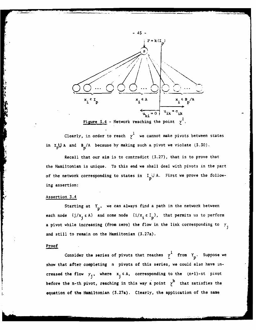
-4S-
i ..//\ ".
x xCI x EA x. EB /A
-u.Uki = 0 ik ik
1Figure 3.4 - Network reaching the point y
1Clearly, in order to reach y we cannot make pivots between states
in IpU A and B /A because by making such a pivot we violate (3.30).p
Recall that our aim is to contradict (3.27), that is to prove that
the Hamiltonian is unique. To this end we shall deal with pivots in the part
of the network corresponding to states in I U A. First we prove the follow-p
ing assertion:
Assertion 3.4
Starting at Y , we can always find a path in the network between
each node {j/x. cA} and some node {i/x.i Ip }, that permits us to perform
a pivot while increasing (from zero) the flow in the link corresponding to y.
and still to remain on the Hamiltonian (3.27a).
Proof1
Consider the series of pivots that reaches y from Yp . Suppose we
show that after completing n pivots of this series, we could also have in-
creased the flow yi, where x. j A, corresponding to the (n+l)-st pivot
bbefore the n-th pivot, reaching in this way a point y that satisfies the
equation of the Hamiltonian (3.27a). Clearly, the application of the same

- 46 -
barguments to the new series of pivots that reaches y from Y provides
p
us with the induction step that proves our assertion.
For the sake of clarity the following notation will be used:
(i)Y J =the slack variable y. that increases (from zero) in the i-th pivot.
2yi)" = the slack variable that decreases its flow in the i-th pivot.
= the costates corresponding to the slack variables of the i-th pivot.
y(n) = the point reached after the n-th pivot.
AY = the increase of flow in a slack link after pivoting.
Suppose we cannot perform the (n+l)-st pivot before the n-th one.
Clearly, this occurs only when there is at least one link common to the n-th
and (n+l)-st pivot cycles, such that the execution of the (n+l)-st pivot is
possible only after the n-th one. All such "critical" links must be in
opposite directions on the n-th and the (n~l)-th pivot cycles. We shall
contradict our assumption by showing that:
(a) (n+l) =(n)
(b) before the n-th pivot there exists a cycle that permits increasing
(n~l) while decreasing yn)
Consider first the situation before the n-th pivot, (see Figure 3.5).
Suppose that (k,j) is the first critical link on the (n+l)-st pivot cycle.
Clearly, since the link is critical it belongs also to the n-th pivot cycle.
Then follow the (n~l)-st pivot cycle from y1nl) up to the node k and
(n)then the n-th pivot cycle up to y2 Clearly we can perform a pivot on
this cycle. Moreover, X(n+ l) < A(n) because if X(n l) > (n ) then, per-
forming the pivot corresponding to this cycle will give:
- 47-
X. (tp)y. (n-1) + X. (tp)y.(n-l) + A(n+l) y+ A (n)Ay = a+ (X (n+l) X (n))Ay a,x EI p I xcA1 ' P
thus, contradicting the optimality of the Hamiltonian (3.27a).
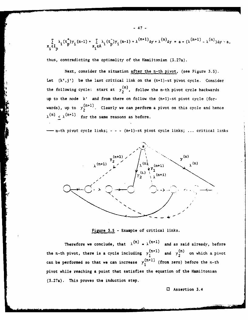
Next, consider the situation after the n-th pivot, (see Figure 3.5).
Let (k',j') be the last critical link on the (n~l)-st pivot cycle. Consider
the following cycle: start at y(n), follow the n-th pivot cycle backwards
up to the node k' and from there on follow the (n+l)-st pivot cycle (for-
(n+ 1)wards), up to yn2 . Clearly we can perform a pivot on this cycle and hence
A(n ) < X(n + l) for the same reasons as before.
-- n-th pivot cycle links; (n+l)-st pivot cycle links; ... critical links
(n+n) W ¢ n (iY2 -dy
(n+l) X (n+1) ,jn)-i . 4Y1
Yr. X(n+i)
Figure 3.5 - Example of critical links.
Therefore we conclude, that A(n) . X(n+l) and as said already, before* (n~l) (n yn) o hc io
the n-th pivot, there is a cycle including yl and y( on which a pivot•(n. 1) ro eobeoetenh
can be performed so that we can increase yl (from zero) before the n-th
pivot while reaching a point that satisfies the equation of the Hamiltonian
(3.27a). This proves the induction step.
0 Assertion 3.4

- 48 -
Now we contradict (3.27). By assertion 3.4, starting at Yp, we can
reach points y* by performing a single pivot on the network. These points
lie on the (IpU A)-face and also satisfy the Hamiltonian equation (3.27a),p|
namely:
7 A.(tlY)y+ X 1 (t)y* = a, Vx eA . (3.31)X.CI 1 p1 In m I p mxII1 p
We check now the second Hamiltonian (3.27b) at the above points.
Notice that since we assumed that (3.27b) is optimal over V, it must satisfy:
Si(tp)y! X 2 (t )y* < a, Vx EA (3.32)X.el 1 p 1 In p MD m
1 p
From (3.31) and (3.32) follows that:
A 2(t) < x t, Vx LA . (3.33)mp-mp m
But obviously, assertion 3.4 holds also for the second Hamiltonian (3.27b), hence:
1(-) 2-) xeA(.4
Thus, from (3.33) and (3.34), we have:
1 (t-) 2 A C), 'x L A
We then conclude that the B -positive-face is unique and therefore the leave-
the-boundary costates are unique.
When only some of the states leave the boundary, we consider the re-
stricted Hamiltonian:
H pItp): z(t ) = i (t+ )yi + A.(t)y'xi p xicLp
with L C 8 . But in order to satisfy the necessary conditions the optimiza-
p p
tion must be global, namely:
H (t-) * H(t) RP pp-l p p
where
-49-
a = cardinality of IP p
P p cardinality of L ,P p
and the basis vectors of JR*p are the elements of I Therefore the
values of the leave-the-boundary costates in the case of L C B are identi-P P
cal to those corresponding to the case of B so that they are unique.p
0 Theorem 3.1.
Theorem 3.2
If the values of the costates corresponding to states travelling on
boundary arcs during the interval between two successive junction times
tp 1 and t are equal to the leave-the-boundary costate values, thenp~l p
every costate satisfies exactly one of the following conditions:
S ( T) = X.(T) = 0, VT e p,t 1 ) , (3.35a)
() =-; Ai (T) > 0, Yt E (--,t p+) (3.35b)
Moreover, in every feedback control region there always exists an optimal
control satisfying y > 0.
Proof
Every optimal trajectory in the state space is characterized by a
control switch time sequence (tf~tf ... ,t t tp,...), when each
switch time represents a transition between two neighboring feedback
control regions in the state space (see (Ml]). The interval between two
successive switch times tp 1 and tp is characterized by the set of
states travelling on interior arcs, I . Considering every possible control
switch time sequence insures that we have traversed every feedback control
region, thus covering the whole state space. To prove the Theorem we shall
consider a typical control switch time sequence, and we will prove by induc-
tion that the costate trajectories satisfy (3.35), and also that there exists

- 50 -
at least one optimal control for which y > 0 within every feedback control
region. Notice that the existence of such an optimal control allows us to
consider only the set of trajectories for which there is no return to the
boundary of states (x = 0), backwards in time.
Now we proceed with the proof. Consider first the interval (tp tp 1).
Since {Xi(tf) = 0, Vx i F Lf} (see [M2], pp. 25-26), at tf all costates
corresponding to the states in Lf are identical. Now, by Theorem 3.1, for
the costates corresponding to states on the boundary to be at their leave-the-
boundary values, we have to find the maximal set of states Afl1 that satisfies:
Max{ I Y i + y.) = Max I yi = k(Lf) (3.36)V xieL f xicA f1 Y xiEL f
Moreover, the enlarged Hamiltonian at tf must lie on V in such a way that
all operating points in Yf-1 satisfy equation (3.36). But as said before,
all costates corresponding to states in Lf have the same value at tf, so
that the enlarged Hamiltonian will contain the (Ifl U Af-l )-face (3.36).
Hence Theorem 3.1 implies that
i) Ai(tf) = 0 for all x. e Bf1 /Af1
(ii) the values of all Xi(tf) are identical for all i such that
xi e L fUA f_11
where (i) follows from Assertion 3.3, and (ii) follows from Assertion 3.4 and
the fact that all costates corresponding to states in Lf have the same value.
Now, clearly there exists at least a point on the (If-l A .l)-face, satisfying
Yi > 0, Yx i eLf = I.1
(3.37)yi a 0, V xi B f
Moreover, since we require that all costates corresponding to states travel-
ling on boundary arcs in the interval (tf~t f1) be at their leave-the-boundary

l- 51
values, (i) and (ii) hold for all Tc (tftfl), so that the point (3.37) is
an optimal solution for all - e (tftf1 ). Therefore we have:
X (T) f f-1, Vx i -L f fU A f 1 -IU Af-i(3.38)
(T) (T Bf 1/Af-1
ST C (tf-t f.I)
Now we perform the induction step: Consider the time interval
(t ,t ), and assume that the set of operating points Y , contains at
least one point satisfying:
y, > 0, Vx. E I
1Yi 0 1 p
We denote by A the maximal set of states satisfying
Max{ I y yi } = k(Ip)Y x.eI x.eA
1 p i p
Keeping the costates corresponding to states in B at their leave-the-
boundary values at every instant on the interval will result by Theorem 3.1 in:
X() - 0,Yxi x- B/A p (3.40a)
X = X(T) V X i Ap x. CI p (3.40b)
Moreover, from the existence of a point satisfying (3.39) during the entire
interval follows that:
A.(T) = X -1,I(3.41)
V T C (tptp +1 )
therefore from (3.40) and (3.41) we have:
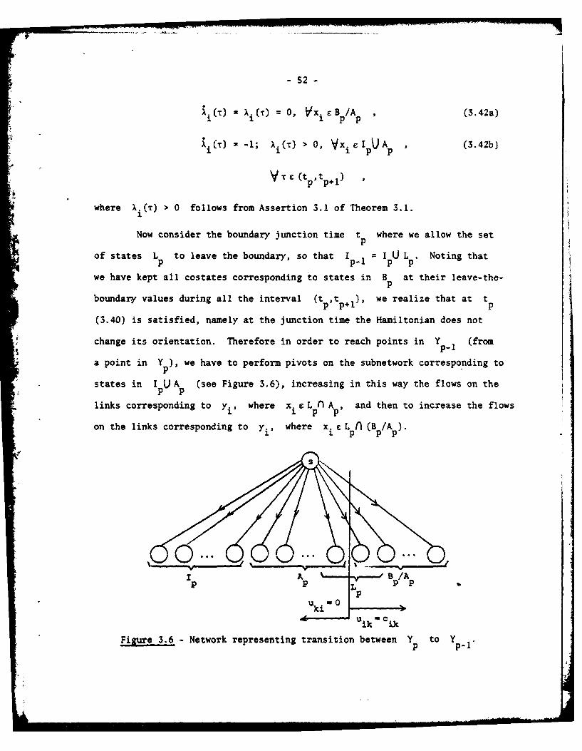
- 52
x. (T) X (') 0, Vx i : B p/A , (3.42a)
Xi(T) - 1; A i) > 0, V x. IUA , (3.42b)1 P p
V rc(t ptp+I )
where X. () > 0 follows from Assertion 3.1 of Theorem 3.1.
Now consider the boundary junction time t where we allow the setp
of states L to leave the boundary, so that Ip 1 = IpU Lp. Noting that
we have kept all costates corresponding to states in B at their leave-the-
boundary values during all the interval (t p,tp+l ), we realize that at tp
(3.40) is satisfied, namely at the junction time the Hamiltonian does not
change its orientation. Therefore in order to reach points in Y (from
a point in Y ), we have to perform pivots on the subnetwork corresponding top
states in Ip U Ap (see Figure 3.6), increasing in this way the flows on the
links corresponding to yi, where x. e Lp A and then to increase the flows1 p
on the links corresponding to yi, where xi c L p( (B A ).
A B p/A p
iL
1
1p p p p
IPU k i 0
, %i
Figure 3.6 - Network representing transition between Yp to Yp-
p pik- ii
- 53 -
As a result of the increase of flow on a link yi corresponding to an
x. Lp (A p, there is a decrease of flow on some link y. corresponding to an
x. C Ip, however, it is clear that we can always increase the flow on y. in
such a small amount that y will still remain nonnegative for all x. £ I3 P
Moreover, the increase of flow on links y. corresponding to x. e (Bp/A )y L1 pp p
does not result in decreases of flows on other slack links so that Y will
contain points satisfying
yi> VxiCIp-1
(3.43)yi 0 Yxi Sp- I
Now IpC Ip I so that when maximal flow is achieved on the network
corresponding to I (i.e., network with slack links y. for all xi e Ip-l 1 1 p-1
only), all minimal cuts of I will be filled. In addition, the sets Ip p
and I U A have the same minimal cuts, therefore:P
ApC A _U Lp (3.44)
where Ap 1 is the maximal set of states satisfying
Max{ I y i + I = k(p-1 )V x.c¢pI xcAp.
i p-1 i ep_
Now, from the existence of a point satisfying (3.43), and from the
same considerations as in the interval (t p,tp+ ), we have
(T) A i (T) -0 V xi BP- 1/A_.1
1C 1 1 p- p-
(3.45)C r) - -1; ?i(r) 0 ; VxeIc 1pUA _
V re (tp13t, p).
Moreover, since I p-l' from (3.45) follows that
X ( ) -- ; >-0• ; .tp (3.46)
T 9 (tp-1,t p

- 54 -
and since Lpr_ Ip_ 1 , from (3.44) and (3.45) follows that:
W - -1; i() > 0, Vx i eA p
(3.47)
Therefore, equations (3.39), (3.42), (3.43), (3.46) and (3.47) provide the
induction step that proves the theorem.
03 Theorem 3.2.
The costate trajectories (3.35) satisfy the necessary conditions (which
are also sufficient) derived in [M2]. Moreover, these trajectories were
obtained by checking at every moment the global Hamiltonian, thus insuring
that values of the costates corresponding to states on the boundary can always
be found such that the solutions obtained by considering only the restricted
Hamiltonian are also globally optimizing solutions. The above arguments yield
to the foIlowing corollary:
Corollary 3.2
Any solution to the constrained optimization problem (see [M2], p. 64)
is also a globally optimizing solution.
O3 Corollary 3.2.
Theorem 3.3
The set of optimal controls does not switch between boundary junction
times; that is, there are no break points between boundary junctions.
Proof
Consider the time interval (t ptp+ ) and denote:
Max xi ()y a( ')o x1 c CIp
Now consider the times T Ct , t +). The set of operating points is given by
p
YpTcl t ha Y/ p t i)yi - a(Tl3 ) si.48)" x. I
IppRecall that all points in (3.48) satisfy
yi k(Ip ( 3.49)
Now consider the time T2 e (t ptp+l), where T2 = T1 + AT. The set of operat-
ing points is given by
~aYp(r 2) - (y CV/ i = a(T2)}1 R p . (3.50)x.cI
ip
But every point in (3.50) satisfies (3.49), and also by equation (3.42b) we
have
(T)= -1, i I p
Y T (t ,(tp. I )
Therefore:
Max I )i(T 2 )Yi = Max{ I . Xi(Tl)yi• AT s) Max X Ai( 1 )yi + A' k(Ip)xicIp Y xi Ip xi lp Y x.eI -
Thus:
Sp(l) I= Y p(T 2 ) .
so that the set of optimal controls does not switch between boundary junction
times.
3 Theorem 3.3.
Theorem 3.4
There is one subregion per region with respect to any set of state vari-
ables leaving the boundary.
Proof
Consider the feedback control region Rp constructed from the set of
-56-
optimal solutions Y on (--,tp). Also, let L be the set of state vari-
ables which we choose to allow to leave from R backwards in time, wherep
L pC B p. According to the definition of subregions (see [M2], p. 57), we must
show that the state variables in L leave with the same set of optimal controlsp
from every point of R . Recall that by Theorem 3.3 the optimal trajectories
associated with the state variables in Lp leaving Rp, do not experience
a break as time runs to minus infinity, so that to prove that there is one sub-
region per region is equivalent to showing that the set of optimal controls
associated with the state variables in L leaving the boundary is the sameP
for every boundary junction time t c (--,t ). Note that we need not be con-p l
cerned with the common breakwall sequences (see [M2], p. 56), since by Theorem 3.3
there are no breakwalls. Now consider two different boundary junction times,
t p, t P2 (--,tp+l) and assume that t > t P. By Theorem 3.3 we have that
ap+PYpI(tPl) l i Y/ I. i(tp )yi
= a(t p)}O R P1
p-lU A 1
and
Y P 1 (tP2) = (yeV/ IP - (t P )y = a(t )}IR P p (3.S2)
p-p2 I, 1 UA 1 _1 p2 1 P2
where
a() - Max X. (T)y i
V I1 UA 1 1~
a +The coordinates of R 'p
P are the elements of Ip-11 and Ap- is defined
as in Theorem 3.2.
Now, by Theorems 3.2 and 3.3 we know that
i(T) -1, VxiCI p U Ap
Xi (T) 0 0, y x i C Bp/A
where Ap is defined as in Theorem 3.2.

- 57 -
Hence:
A (t P2) = A i(t f ) 0, Yx i E (I piU A p_)/(Ip A p)
Xi(t P2) = Xi(t p) + tPl , tP2)' V xi E I p Ap
therefore
Max A.(t )y. = Max{ .(t )y i (tp-tp) y}Y I p I P 2. Y IpPi PAp .1 I p A p _
= Max A i(tp )Yi + (t p-t )k( p_1
V Ip1U Ap_ 1 1 1 P2
so that
Yp1 (t) = Yp- 1 (t) ,
then the set of optimal controls associated with state variables in Lp
leaving the boundary from Rp. is the same for every t e (--,t pl).p p4.
0 Theorem 3.4.

58
Section 4
1NE ALGORITHM
This section is devoted to the description of a simplified algorithm
for building the feedback solution to the minimum delay dynamic message rout-
ing problem for single destination networks with all unity weightings in the
cost functional. The simplifications obtained arise from the special proper-
ties of these kind of networks, as discussed in Section 3, and from the new
approach to solve the linear programs presented in Section 2.
In Part A we state the algorithm while explaining its steps. In
Part B we present a method for obtaining all optimal solutions of the linear
programming problems required by the algorithm and finally Part C brings an
example that provides a good insight of the performance of the algorithm.
A. Statement of the Algorithm
Operation 1
List all possible trajectories in the state space, by writing all pos-
sible sequences of states leaving the boundary backwards in time.
E Operation 1.
Recall that every optimal trajectory in the state space is character-
ized by a control switch time sequence. Each switch time represents a transi-
tion between two neighboring feedback control regions. Now by Theorems
3.2 - 3.4 there are no returns of states to the boundary, there are no breaks
in the optimal controls between junction times and there is only one subregion
per region. Therefore every trajectory is characterized only by departures
of state variables from the boundary, the boundary junction times might be
arbitrarily taken and between two successive boundary junction times the set

59-
of optimal controls does not change. Thus, Operation 1 takes int: ac:ount ai
possible trajectories in the state space, so that the construct:on cf reedbak
control regions based on these sequences insures a complete coering f the
state space. Such a typical sequence looks as tollows:
[ f ,I f), "",tL pI 'tL p i b l, _ '1 L f -n - l1
The number of possible sequences Q(n) is given by (see (Eli, p, 68).
n r=' V E (-1) ir r~L "H)I (r';)ni
r=l i=o
nNotice that the complexity of Operation i is of the order of nn, so
that clearly the algorithm is implementable only for "small" netwock!
Example 4.1
Consider a network with three state vaiables x1, x2 and T3 rhe
sequences are:
tf tf.1 tf 2
I. x2 3
2. xI x3 2
3. x (x2,x3)
4. x2 xI x3
S. x2 x x
6- x2 (x1'x3)
7. x3 Y1 X2
8. x3 X 2 x1
9. X3 (X1 ,X2 )
10. (Xlx 2) x3
11. (xI X 3) x2
12. (x2Px3) xI
13 Xlgx 2,x3) "L Exhale 4.

60-
Operation 2
Derive the networks corresponding to every possible combination of
state variables leaving the boundary. Apply the algorithm of Maximal Flow to
the networks and find the corresponding flows.
0 Operation 2.
From Operation 2 we obtain the first optimal solutions to the linear
programs (as explained in Parts B and C of Section 2). Also, the operation
provides the essential tools for obtaining the simplifications of the algor-
ithm as will be shown in Operation 3.
The nuner of networks for which the Maximal Flow Algorithm is to be
applied is 2n-1 . The complexity of this operation is therefore exponential
in the number of nodes.
In Appendix B we provide a computer program in Fortran for finding
the maximal flow in these networks, based on the algorithm of Edmons and
Karp (see [Hl]).
Example 4.2
All the possible combinations of states leaving the boundary in
example 4.1 are:
{xl},{x 2},{x 3},{xx 2},{l,X 31,{x 2 X3 },{XlX 2 ,X3 }
03 Example 4.2
Operation 3
For every sequence of state variables leaving the boundary listed in
Operation 1, and considering the results obtained in Operation 2, execute the
following steps:

- 61 -
(a) Consider every set L of the sequence and check if there is a sub-P
set of states B such that B C L, and such that there is a set B'
where I U B c B', and such that the same value of maximal flow
corresponds to both sets, I U B and B'.~P
(b) If (a) is satisfied, check if in a set Lq of the same sequence,
where q < p there is at least one state variable x. such that
x. e B'/(I U B).J p
(c) If (b) is satisfied, erase from the list of Operation 1 the sequence
being currently checked.
0 Operation 3.
In order to justify Operation 3, consider first the following notation:
S I}., { I p-I(B)} ,... (4,1)
The sequence (4.1) represents all trajectories in the state space character-
ized by the sets of states travelling on interior arcs in every time interval.
In (4.1), the notation ( Ip 1 (B)) means that the set of states B is such
that B C L, that is, the states in B leave the boundary at t p. Notice
that B C I .
Now consider the following sequence satisfying (a) and (b):
(I .} . .{ p}), {I p-1(B)}...{I q},{(I q-l(X j 1} ,Ilq 2} ,I... (4.2)
where xjcB'/(IpUB)
Now consider the following sequence:-
(If-l 1,.. ,p, {Ip-l(B)),...,{Iq JX),{Iq-ll Iq.2},... (4.3)
The only difference between sequences (4.2) and (4.3) is that in (4.2),
x. leave the boudary at tq while in (4.3) x. leave the boudary at tq.l ,
Notice that the existence of a sequence as (4.3) is insured since Operation I

-62-
requires the listing of every possible sequence.
We claim that all feedback control regions constructed from sequence
(4.2) are also constructed from sequence (4.3) so that sequence (4.2) is redun-
dant. The reasons for that appear in the following argunents:
By the considerations of Part D in Section 2, we know that in order to
find all optimal solutions (to construct the corresponding feedback control
region) corresponding to the time interval (t ,t ), we find all optimalg+l gsolutions corresponding to the states in Ig leaving the boundary, and among
these solutions we choose those that maximize the expression
X A (t g) .
ig
Now it is-not difficult to see, that by Theorem 3.2 the costate values in both
sequences (4.1) and (4.2) are the same at all times. Moreover, note that if
all optimal solutions corresponding to the states in I U B leaving the boundaryp
are also optimal solutions to the problem corresponding to the states in B'
leaving the boundary, then all optimal solutions corresponding to the states in
I U BU D leaving the boundary (for some set of states D) are also optimalp
solutions of the problem corresponding to the states in I V B VD VE leavingp
the boundary, where E CB'/I U B. The above is easily seen by noting that all
minimal cuts corresponding to I U B are also minimal cuts of the network cor-P
responding to I pU B U E, therefore all minimal cuts corresponding to I pU B U D
are also minimal cuts of the network corresponding to I pU B U D U E.
Now returning to sequences (4.2) and (4.3), we have that
1 2 . I 1 I Vx. (4.4)q q j
(where I1 and 12 denote the sets of states travelling on interior arcs inq q
the tim interval (t q+li t q) in sequences (4.2) and (4.3) respectively).
LMp

- 63-
Moreover we can write
1 11 q (Iq/I pUB),'I UB , (4.5)Iq qpp
so that from (4.4) and (4.5) we have
2 1I (Il/I C B) U I UBUx. (4.6)q q p p 3
But from the above reasoning all optimal solutions corresponding to (4.5) are
also optimal solutions of the problem corresponding to (4.6), moreover:
g g
Therefore the sequence (4.2) is redundant.
Example 4.3
If in example 4.2 we obtain the same maximal flow value in the cases
corresponding to the sets of states xI and (xlx 2,x 3 l leaving the boundary,
then we erase from the list of example 4.1 the sequences numbered (1), (2), (3),
(4), (7), (10) and (11).
0 Example 4.3.
Operation 4
For every state variable combination Lf leaving the boundary at tf
for which there is not a combination L' such that Lf C L' , and the maximal
flow values corresponding to both combinations are equal, find all the optimal
basic solutions of the corresponding linear programming problem starting with
an optimal (extended) basic solution as explained in Parts B and C of Section 2,
and using the algorithm provided in Part B of this section.
O Operation 4.
The results obtained from Operation 4 are the basic data needed for con-
structing feedback control regions (the construction is carried out in Opera-
tion 5).kMai

- 64 -
Operation 5
For every remaining sequence (after execution of Operation 3) from the
list of Operation 1, carry out the following steps for every boundary junction
A - time t , in a sequential order, starting at tP f
(a) Set
X. (Tr) X -1 EI x. £-% 1 p-i
T (--,t p)
- 0, 'vx i Bp. 1
T1 t P19 p-
with
Ai(tf) = 0, {xi/ieN}
(b) Set arbitrarily t - t = 1p p-i "
(c) From among all solutions {y*} obtained in Operation 4 with Lf = Ip- 1
choose those that maximize the expression:
A i (t -)y
(d) Transform the solutions obtained in (c) to the set of rays V (see
[1], p. 58) and construct the convex polyhedral cone:
where C (.) denotes the convex hull.
(e) Consider all sequences that are identical to the current sequence
until the current time interval (t 1 ,t). The costate values of
such sequences in interval (t p19 tp) will be identical to the co-
state values corresponding to the considered sequence, and the cor-
responding feedback control region will be built only once. This

- 65 -
insures that we avoid multiple construction of the same control region.
3 Operation 5.
Step (a) follows from the costate trajectories depicted in Theorem 3.2.
Notice that in the sequences left after Operation 3, the costate x starts
to change only from the boundary junction time in which its corresponding
state leaves the boundary, so that the calculation of the costate values is
an easy task. Step (b) follows from the fact that there is only one subregion
per region with respect to any set of state variables leaving the boundary (as
proved in Theorem 3.4), so that we may arbitrarily choose the boundary junction
times. Step (c) follows from Part D of Section 2. Step (d) follows from the
Constructive Dynamic Programing Algorithm stated in [2]. Finally, step (e)
is a simple conclusion that saves superfluous computational work.
B. The Method for Finding all Solutions
to the Linear Programming Problems
One of the major problems in the implementation of the algorithm
described in Part A of this section arises from the need of finding all solu-
tions to every linear program required in Operation 4 of the algorithm. In
geometrical terms, the problem is to find all the extremal points of the con-
vex polyhedron formed by the intersection between the enlarged Hamiltonian
and the X-constraint figure lying in the positive orthant of the y-space.
Fortunately, the above linear programs are in general highly degenerate so
that as it was clarified in Part C of Section 2, the number of finear programs
we actually have to solve is greatly reduced.
The problem of finding all solutions to linear programs has been
widely investigated. See for example [Bl], [Chl], [Ch], (M4], (R1]. In [B2],
we find a report on computational experience gained using the algorithms
- 66 -
presented in [Chl] and (Ch2], as applied to optimal routing problems. From
this report it is seen that even for very small size networks the amount of
computation and memory required is excessive, and also the numerical sensitivity
of the algorithm is extremely high.
We proceed now with the description of the method to find all the solu-
tions of the linear programs that we propose and later we shall discuss its
advantages. The algorithm is based on the method of pivoting on networks.
For a review of this method the reader is referred to Appendix A.
Starting at an optimal extended basic solution, the algorithm picks a
nonbasic link and looks for the cycle formed by basic links and the considered
nonbasic link. There always exists such a (unique) cycle since every extended
basic solution corresponds to a spanning tree in the network. In order to
find the cycle the algorithm utilizes a labeling technique that will be
described later on. After finding the cycle we perform a pivot on it, reach-
ing in this way either a new extremal solution or, if the cycle is degenerate,
another representation of the original extremal solution. If the degeneracy
is of a high degree, we may find with a single pivot several different representa-
tions of the extremal solution. Every new solution or representation obtained
is numbered and kept in memory if and only if it does not exist there already.
The above process is performed for all nonbasic links corresponding to every
solution and/or representation kept in memory until it is not possible to
reach a new solution or representation. In this way we insure that at the
end of the process we had reached all optimal solutions. Since we are not
concerned with different representations of extremal solutions when construct-
ing feedback control regions at the end of the process, we can delete these
representations retaining only one representation per extremal solution. In
order to start the process, we reach an initial extended basic optimal solution
as depicted in Parts B and C of Section 2.

- 67 -
Now, to understand the need of searching also the different representa-
tions of every extremal solution, let us consider the following example.
Example 4.4
Given the network depicted in Figure 4.1, the problem is to find all
optimal solutions corresponding to all states leaving the boundary.c c21 2 c 3 2 =2
Figure 4.1 - Network of Example 4.4
After finding the minimal cut of the network (recall that to find a
first optimal basic solution, we add a new node (the source) and links with
no capacity constraints connecting the source with every node of the network,
and we apply the maximal flow algorithm), we choose the first basic optimal
solution shown in Figure 4.2-a. From this solution and by pivoting on the
cycle corresponding to the nonbasic link (3,2), we reach another extremal
solution as depicted in Figure 4.2-b. Note that from the first solution,
pivoting on the cycle corresponding to the nonbasic link (s,2) does not lead
to a new solution but just to another representation of the first optimal
solution. Clearly, from the representation of the extremal solution of
Figure 4.2-b we cannot reach a new extremal solution. Only starting at tie
representation shown in Figure 4.2-c can we reach the new extremal solution
depicted in Figure 4.2-d.

-68-
I 0
S, 0
(~ ~- --- ;- <
(a) (b)
- - - - nonbasic link
basic link
0S
0 f20
....3 ,- - -- N 03-- -0 0 2 0
(c) (d)
Figure 4.2 - Obtaining extresml points in the network of Example 4.4.
O Example 4.4.
Iot w.e describe ;te labeling technique used by the algorithm to find
pivot cycles. First we assign a number to every node and link in the network.
For example see Figure 4.3:
/3
8
67 9
Figure 4.3 Nubering nodes and links.

- 69 -
Second, we define the following arrays:
C(I) = Capacity of the link I.
F(I,J) - Flow on the link I at the J-th solution.
BASE(I,J) = Type of the link I (basic or nonbasic) at the J-th solution.
LOUT(I) = Exit node of link I.
LIN(I) = Entrance node of link I.
where:
1 if the link I is basic
BASE(I,J) =
0 if the link I is nonbasic
Now if link K is nonbasic, in order to find the pivot cycle we search the
arrays LOUr(I) and LIN(I) and we find all the incident links to node
LIN(K) (where LIN(K) is the entrance node of the link K). After find-
ing all these links we consider only those that are basic, and for every one
of them we carry out the same procedure until we obtain a basic link entering
(exiting) into (from) node LOUT (K). To every link searched in the above
procedure, the number of the preceding link of the cycle is matched so that
at the end of the procedure a well-defined cycle is obtained. After finding
the cycle, and by checking the arrays C(I) and F(I,J) we obtain the maximal
change of flow on the cycle and we perform the pivot. As said before, when
the cycle is degenerate, we reach all possible different representations by
performing "dummy" pivots, that is declaring the nonbasic link as basic, and
the basic link that does not allow to change the flow as nonbasic.
Standard labeling techniques assign ntmbers only to the nodes of the
network so that the links are identified by a two-dimensional array (I,J),
where I is the exit node of the link and J its entrance node. However,

-70
note that in order to use this technique we must define in our case two arrays
that are three-dimensional, the first accounting for the flows on the links,
the second for the type of links. kreover a two-dimensional array for the
link capacities is needed, thus making use of an excessive and wasteful
amount of memory, especially when the number of solutions and representations
is large. Clearly, by defining only two-dimensional arrays (as we do) we
save a large amount of memory. Notice also that, when finding all the solu-
tions to the linear programs by means of pivoting on networks, every solution
or representatiou is identified by a solution vector and a link-type vector
instead of a tableau (as is done when utilizing simplex methods) saving again
a great deal of memory.
The main problem of the method is that we do not know a priori the
number of solutions and representations of the linear program, so that we do
not know the dimension needed for the arrays that will contain the solutions
or representations. Truly, we can find an upper bound to the number of solu-
tions and representations since every basic solution corresponds to a spanning
tree and it is possible to calculate the number of spanning trees in the net-
work, however, not every spanning tree corresponds to a feasible basic solu-
tion. For example, in the network depicted in Figure 4.4 a non-feasible span-
ning tree is shown.
- - -.... nonbasic link
Us2 -2basic link12 4= . 2
- -2Sb i - -2 b 2 m--2
Figure 4.4 - Example of a non-feasible spanning tree.

- 71 -
Therefore, in general, the number of feasible solutions is less than
the number of spaming trees, and for practical purposes the dimension of the
arrays having a coordinate defining the number of solutions and representa-
tions is estimated and fixed accordingly.
We present now several examples that will test the efficiency of the
method. All examples apply to the case when all the states leave the botudary
(that is, the case in which we obtain the maximal number of solutions) and
they were solved by means of a Fortran computer program (see Appendix B)
based on the method described above. All programs were run on an IBM 370/168
computer, and for every example the maximal memory region provided was S12K.
In Figure 4.S we show the tested networks with the corresponding
numbers of optimal solutions and representations, and the CPU time consumed.3
N3 Number of solutions: 24
Number of solutions4 and representations: 48
CPU time: 1.78 sec.
(a)
2 r ,. . Ntm~er of solutions: 202Number of solutions
and representations: 582 CPU time: 1.59 sec.
(b)

- 72 -
2 3 4 Number of solutions: 60
Number of solutions
3 4 2and representations: 156
CPU time: 5.41 sec.
(c)
1 6 5
334 Number of solutions: 34
Number of solutions4 and representations: 78
CPU time: 2.2 sec.7d
Cd)
1 5
3 5) Number of solutions: 68
Number of solutions
6 2 and representations: 184
CPU time 7.41 sec.
(e)
Figure 4.5 - Example of finding all optimal solutions.
From the examples of Figure 4.5 we obtain an insight into the change in the
number of feasible spanning trees when changing capacities of some links (see
4.5a and 4.Sb) and the great increase in the number of feasible spanning
trees when adding a single link to the network (see 4.5b and 4.5c, 4.5d and
4.5e).

73-
Note that since the capacities are integers and the only arithmetical
operations in the method are additions and substractions, no numerical sensi-
tivity problems arise.
Now we anal .ze briefly the complexity of the method for finding all
optimal solutions. Consider first the non-degenerate case, that is, the case
in which every optimal solution satisfies:
yi > 0, i = 1,2,...,n , (4.7)
where n is the number of nodes in the network. Denote also by t the
number of links in the network. Clearly, if (4.7) is satisfied at every
optimal solution, the links corresponding to the slack variables "y" are basic,
and the remaining links are non-basic. Since the flow on a non-basic link
(ij) must be only zero or ci, the number of optimal (basic) solutions
is 2(1-n). This explains the great increase in the number of solutions when
adding a single link to the network. In the degenerate case we can only
estimate an upper bound for the number of solutions and representations. This
upper bound is given by multiplying the number of spanning trees of the net-
work by 2(L-n). The conclusion arising from the above arguments is that
owing to its exponential complexity the method can actually be implemented
only for relatively small networks.
C. Example of Feedback Solution to the Dynamic Routing Problem of a
Single Destination Network with all Unity Weightings in the Cost Functional
In order to illustrate the algorithm described in Part A of this section
we present here an example of a four-state variable network for which we execute
some of the operations of the algorithm. The network is depicted in Figure 4.6.

- 74 -
3
4
Figure 4.6 - Network to illustrate the algorithm.
Operation 1
In this operation we list all possible sequences of states leaving
the boundary. Since there are four states, we obtain Q(4) = 75 different
sequences.
t tf tf tff-3 f-.2 __. It _
x4 x3 X2 Xl
x3 X4 x 2 X* x2 x4 x 3 x1
x 4 x2 x 3 x1
x2 x 3 x4 5.x 3X X 4 X,
x4 x3 x1 x2
x3 x4 , x2
x4 X. x3 x2
X, X4 x3 x 2

-75-
xx 3 x 4 2
x 3X X 4 X2
X4 x2 X, 3
x2 x4 X, x 3
X x x4 X, 2 3
x 2 ,x 4x32 1x 2 4 x3
x 3x 21X 4
X23 X1 X
X 3 X, X2 x 4
3 4
4 X ,X ~3 X4
3 22 X4 X,
X2 x 3 X 4 X,
4X, 3 X2
x4 Xi'X3 X 2
x 4 XVX2 x 3
x2xV'X 4 x 3

-76-
x 1 x 2x4x 3
2c x3 XV24
6 x 1 ,x3 X
x P4x2 "1
xx 4 x3
X2x3 x4X,
x 3$x4 ,x2
XV4x3 x2
x 4 x
7 xV3X,
84 x3x 4X
4 X XV1 X 3
X24 xlVx 3
x 3X xilIx 34
9 X2 x 3 l 4

-77
x4 1X4 2"
x x
3 1 X
Xx 3 ___2_____4
10 x2X
11 x 1 x 2 X3 1x 4
x2,x3,x4 x1
12 X, x ,x4 2
x1,x2,x4 x 3
U-13 X, ' ______4
X2,x 4 X
14X2Vx4 XV1 X3
x1,x4 x 2,vic3
is x1,x 2 x 3 x 4
16 2 X, X39X 4
17 ,x2 S4
x 3 xi__________18 x x2,xx 4

- 78 -
Operation 2
Here we calculate the maximal flow values of the networks corre-
sponding to all possible combinations of states leaving the boundary.
This is carried out by using the Maximal Flow computer program provided
in Appendix B.
In the case where all states leave the boundary, there is no need
to apply the computer program since, as stated in Part B of Section 2, the
solution is trivial (see Figure 4.7).
2 22
Figure 4.7 - Network representing all states leaving the boundary.
The solution is:
Uli m ui6 ci6 , i = 2,3,4,5
uik = 0 k - 2,3,4,S
The value of the maximal flow is 9.

ARC =L 0 CAlAC I TY
(1.4) 0")
(105 2(2,3 0 2.
(2.5) C L(394.) Cl
(3.6) ~(4.3)
(4,5) 0
T-WE VALUE OF THE MAX I MAL FL0, I
ARC FLOW CAPAC I TY
(192) 5 9
(1.4) '
(1.5) 2 .0
(2.3) 2 2
12,5) 0 3(2. v61) 3 ,' .3
(. 44) 0 1
1396) 3 4
(4.3) *
(THE V A 2 * A
T14E VALUE 07 THf MAXIM&IL SnLO"W IS *t
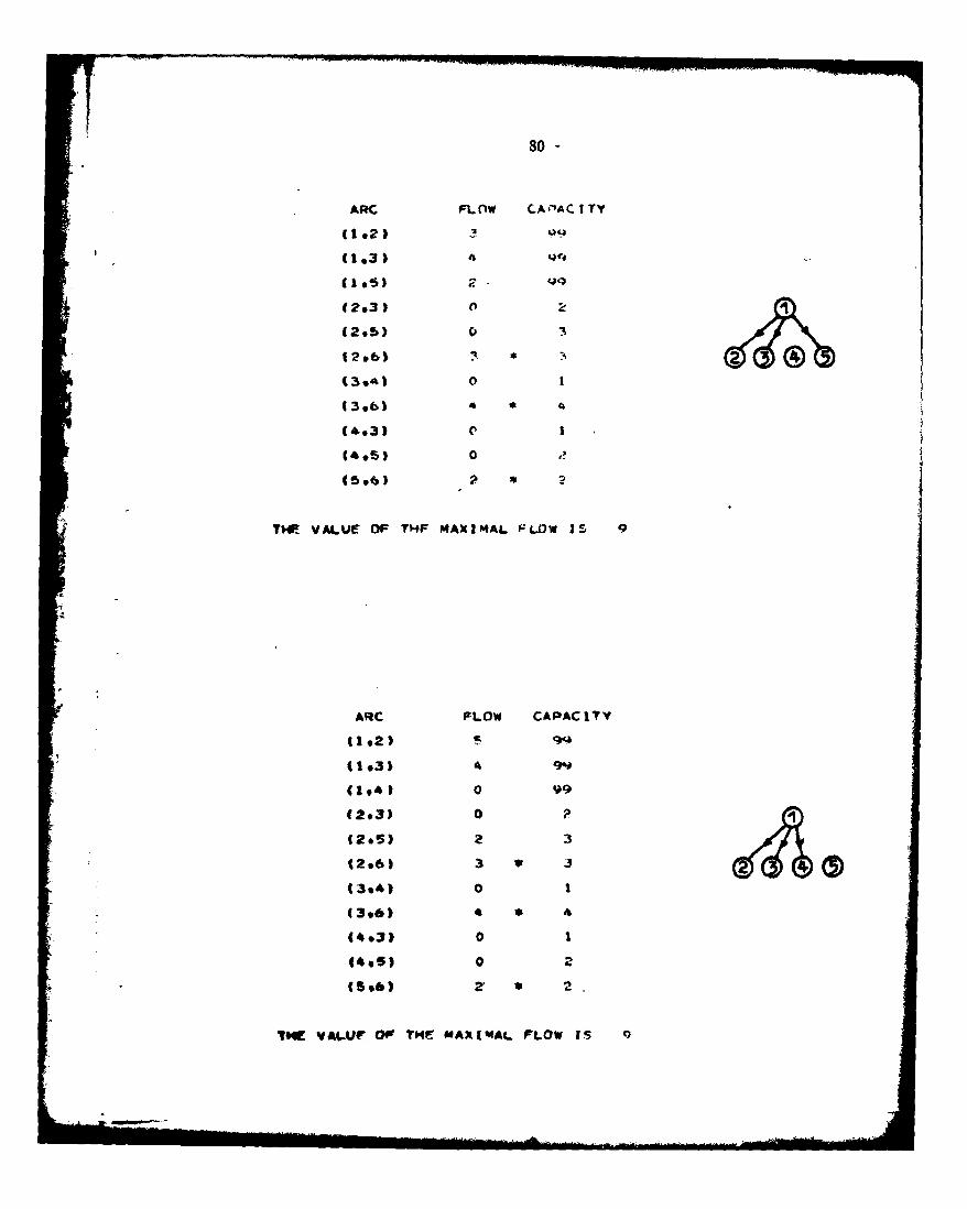
80 -
ARC FL)W CA-'AC ITy
(192) 30(1.3) 4 ,)4
(2 3) -
(2.5) -
12.6) 7 -1
(3,4) 0 1
(3,6) 4 * 4
(4.3) e1
(4.05) 0
(5.6) P * -
TW. VALUE OF THF MAXIMAL F LOW IS 0
ARC FLOW CAPACITY
13) 9I (1,4) 0
(2.3) 0 P
(2.5) 2 :3
(2.6) 3 * J
(3.4) 0 1
(3.6) * * 4
(4,3) 0 1
(4.5) 0 a.
(56) 2 ,
T3E VAL4(J O) TME MAXZAL FLOW IS

-81
AQC FLOlW CA~skC17Y
4104)
(2.3) 0
(2.5) 0 3
(2.6) 0 3
(4*3) 1 1
4.5) 0
15.6) 2
V9 VALUC OF THE M4AXIMAL FLOW IS 3
ARC FLOw CAPACITY
11.3) 4 9
(1.5) 29'
(293) 0
(201%) 0
(2,6) 0 3
1396) 4 1 r*
(3.4). 0 f#
(43)0 t
(4.5)0
(6.6) 2 2
TME VALUIE OW THE MAX104AL FLOW 15 6

S82 -
ARC FLOW CAPACITY
(1 .3) 4 99
1.4) 2-
(2.3) 0
(2.5) 0
(2va3 0(3.4) 0 , 1
(3.6) 4 4
(4.3) 0
(4.5) 2 * 2
(5.6) 2 2
THE VALUE OF TH9E MAXIMAL FLOW I5"
ARC L L)W CAPACITY
(12) 59
(1,5) CA
(2.3) 2 - -
1295) 0 3
(2.6) . * 3
(3.61 2
(4.3) 0 1
(4,5) 0 ?
(5.6) 2 *
TIE VALUE OF THI* MAXIMAL FLOW IS 7

-83
'ARC FLOJW CAPAC IT Y
(2*3) ~(29S) 2
(3e4) C
(3.6) 3
(5.6) 2
THE VALUF Of TME MAXIMAL FLOW IS~
ARC FLOW CAPA~CITY
1 *3) 0
(?.5) 2 ci
(296) 3 * :3
(?06) 4
4493) 0
(4043) 0
(5.6) 2
T9IE VALUE OF THE MAXIMdAL FLOW tS

-84-
APC fL.)w CA PAC ITY
(1.5) . 9'0
(3.6) 4
THE VALUE OF THE 04AXIMAL t-LUWy IS 2
THI S PACX9 IS B.ES T Q3ATJ T-Y M4 "1 71CABLE
ARC FLOW CAPACITY
(2.3) 02
* 12.5) 0
(2.01 0 3.
(394) 0 1
(9.6) 2
THE VALUE OF THE OAXIMAL FLOW IS

ARC KL!IW CAPAC IT'r
(103) 5
(2.6) 0
THE VALUE OW THE 4~AXJP4AL FLOw IS S
P~IS PA.G-;;
AQC FL -W CAPAC I Tv
(1.2) 99
42o3) 2 6 2
2 3
(.3*4) 0
(3.6) 2z
799 VALUE OlP IMF MAXIMAL FLr)W i'D 7

-86-
The links belonging to a minimal cut are marked by asterisks (*) in
each of the above programs.
Now we summarize the results we obtained:
D k(D)
x ,x 2 ,x3 ,x4 9
X1 , 2 'x3 9
x 1,X,x 4 9
xl,x2 9
xI , x3.,x4 8
:* xlx 3 8
x. 1,x4 7
x1 7
x2 ,x3,x4 6
'V" x2 , 3 6
x2 ,x4 6
x2 5
x 3 , x 4 3
x 3 3
x 4 2
This table will assist us in the execution of Operations 3, 4 and S.

- 87 -
Operation 3
In this operation we erase redundant sequences from the list of Opera-
tion 1. The Operation is made by searching all the sequences of the list and
by checking if the conditions of redundancy are satisfied considering the
results obtained in Operation 2.
In our example we obtain that only 18 sequences from the 75 listed in
Operation 1 are nonredundant. These sequences are marked and numbered in the
list of Operation 1.
Operation 4
Here we find all basic optimal solutions for all combinations of
states leaving the boundary. By the sumarizing table of the maximal flow
values we realize that it is enough to find all the solutions for only five
combinations of states. Notice that in the cases where only one state leaves
the boundary the solution is unique, and it is given by the result obtained
in Operation 2. The five networks for which we have to find all optimal
solutions correspond to the largest combinations of states (containing at
least two states) having different maximal flow values.
Using the results of Operation 2 (where we localize minimal cuts) and
by the considerations of Part C of Section 2, we obtain first basic optimal
solutions to every one of the networks, as shown in Figure 4.8.

- 88 -
J87
12
4 0 2 2
2 AJ32 4 5 5,
(a) (b) (c)
4 2 2
3 4-T
(d) (e)
Figure 4.8 - The first optimal solutions
Applying the method for finding all the solutions described in Part B
of this Section (the computer program implementing it is provided in Appendix B),
on the above networks, we obtain the following results:

-89 -
30 0 0 0 0
52 0 0 0 0 0
3 3 1 0 1 0 0
3 4 2 a 0 0 0 2 0
5 4 0 0 0 0 2
5 2 0 0 2 0
720 L. 0 a 0 2
43 4 0 0110 0
3 5 0 1 010 1 0
3 3 3 00 0 1 2 0
5 31 Q ( 0 10
3 51 a 0 2 0
5 2 0 0
0 2 - 1 0
513 0 2 0 ? 0
7 1 1 0 2 0 1 0 2
531 0 2 1 0 2 0
540 0 0 1 1 0 2
45 0 0 0 10 1
3 4 2 0 0 11 2 0
7 2 0 0 p I 1 0 2
6 3 Ci 0 2 0 1
5 2 2 0 2 1 20
WNSMER OF DC1F'rP4T S(1.UTJCNS P 4
~4MSfr OF otFP'ERENT SOLUTIONS AND =!PrcNTTTN
(0)

*fl-AO85 160 MASSACHUSETTS INST OF TECH CAMBRIDGE LAS FOR INFORMA-ETC F/B 17/2
MAY 80 N JODORKOVSKY. A SEGALL N001-75-C-1183
UNCLASSIFIED LIOS-R-88 ,t.
Iommomo I U

D I = 11II1-.2
11111111112-IIIIIIIIo
11111IL 25 111111.4 1.6
MICROCOPY RESOLUTION TEST CHARTIA ,.,AL .... O... .

900
WNVER0 OF LD1FFE~iENT sriLui lrN- 3
MUMSEIR OF O1FCFE9?FNT 'LU I ICN~t AN!) REPPrSNTATIONS:
(b)
'5 2 0
7 0
HUW8FP OF DIWaFrREPT SCLUTT('IONL
NLMBFR OF DIFFFOENT bOLLPTICNL. AND0 PORESE4JTATIONS : p

7--,
91-
(193) ( 1,,4) I19") (.J 94) (49.3) (405)
S 0 0 0 0
3 1 1
2 0 0 .0 2
4 0 2 1 i 0
0 1 1 0 1
3 3 0 1
5 £ L 1 0 2
4 2 2 1 1
NUMBER OF DIPFPRPNT SOLUTIf :
NUMBER OF DIFFEWINT SOLU71ONS AND REPRFSENTATIONS 2 14
(4)
(104 ) (I it-s) f ,,. )
1 2 0
3 0 2
NUMBER OF DIFFERENT SOLUTIONS 2
MUMI E OF DIFFERCNT SOLUTIONS A 4D PRESENTATIONS
(0)
:I(e
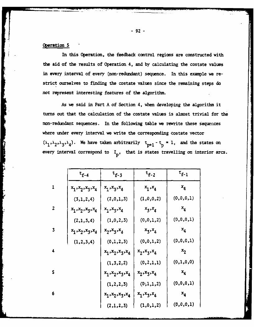
- 92 -
Operation S
In this Operation, the feedback control regions are constructed with
the aid of the results of Operation 4, and by calculating the costate values
in every interval of every (non-redundant) sequence. In this example we re-
strict ourselves to finding the costate values since the remaining steps do
not represent interesting features of the algorithm.
As we said in Part A of Section 4, when developing the algorithm it
turns out that the calculation of the costate values is almost trivial for the
non-redundant sequences. In the following table we rewrite these sequences
where under every interval we write the corresponding costate vector
(, 2,x 3,x4). We have taken arbitrarily tl 1 -tp - 1, and the states on
every interval correspond to Ip,. that is states travelling on interior arcs.
tf-4 tf-3 tf-2 tf-1
1 xl,x2,x3',x4 xl,x3,x4 x4 x4
(3,1,2,4) (2,0,1,3) (1,0,0,2) (0,0,0,1)
2 '1 ,x2 lx3,x4 xl,'x3 x4 x3 'x4 x4
(2,1,3,4) (1,0,2,3) (0,0,1,2) (0,0,0,1)
3 x1 ,x2 ,xx 4 x2 ,x3 ,x4 x3 ,x4 N
(1,2,3,4) (0,1,2,3) (0,0,1,2) (0,0,0,1)
4 x1 ,x2 ,x3 ,x4 x2 ,x3,x4 x2
(1,3,2,2) (0,2,1,1) (0,1,0,0)
5 xl,x 2,x 3,x 4 x2,x3,x4 x4
(1,2,2,3) (0,1,1,2) (0,0,0,1)
6 xl,x2x3,x 4 Xl,X 3 ,X4 N
(2,1,2,3) (1,0,1,2) (0,0,0,1)

- 93-
7 fixp x4 P4X
(2,1,1,3) (1,0,0,2) (0,0,0,1)
8 x lx 2,x3,x4 xV4X
(1,1,2,3) (0,0,1,2) (0,0,0,1)
9 x1,x2,x3,x4 x1 ,x3,x4 X1,x4
(3,1,2,3) (2,0,1,2) (1,0,0,1)
10x. 1 x2 ,x3,x4 x1,x3,x4 Yx3 4
(2,1,3,3) (1,0,2,2) (0,0,1,1)
11 x1,x2,x3,x4 x2,x3,x4 x3,x4
(1,2,3,3) (0,1,2,2) (0,0,1,1)
12 X,x 2,x3,x4 X2
13 xltx2 Px3,x4 X
14 x1,x2,x3,x4 XX
(2,x1,,2 )3,14 0x3 1)
16 XJIX 2 'x 3 'X4 X1 x3X4
17 x1 ,X2,x3,x4 x2"x3 'x4
(1,2,2,2) (0,1,1,1)
18 X1 ,X2,x3,x4

I - 94 -
Section 5
CONCLUSIONS
We presented a new approach for the construction of a feedback solu-
tion to the minimal delay dynamic message routing problem for single destina-
tion networks with all unity weightings in the cost functional. The approach
seems to be the most appropriate one for tackling the problem, since it fully
exploits the special structure of the constraints matrix and also provides a
physical meaning to the problem by working in a framework of networks rather
than in an abstract mathematical one.
Several improvements have been achieved compared to previous results.
The first is the great reduction in the number of linear programs to be solved
by taking advantage of the high degree of degeneracy that in general character-
izes this kind of problems. The second is the derivation of a suitable method
for finding all solutions to the linear programs, that does not require the
application of simplex techniques to achieve a first optimal solution but only
the application of a simple algorithm of maximal flow. Nbreover, the method
reaches all the remaining optimal solutions by pivoting operations on a net-
work, saving in this way a great amount of computer memory. The third improve-
ment achieved is that the new approach provides the tools for analyzing the
complexity of the problem, giving us an idea of the number of computational
steps required for obtaining the feedback solution to a given network.
Further research is required for Operation 1 of the algorithm. Since
not all sequences listed in the above Operation are used for constructing
feedback control regions, the question is whether a method can be provided to
avoid the listing of those sequences not contributing to the construction of

- 95 -
the feedback solution. It also seems that the algorithm my be applicable in
the case when constant inputs are present. Hiwever, further research is needed
to investigate the influence of these inputs on the different Operations of the
algorithm.
Finally, it also remains to extend the application of the approach to
the more general case of multidestination networks.

- 96 -
Appendix A
Basic Concepts of
Graph Theory, Maximal Flow and Linear Programming in Networks
1. Basic Definitions
Directed Graph: A set of nodes N = (1,2,...,n} and a set of directed
links L - {(i,j),(k,x),...,(v,w)) connecting pairs of nodes of N.
Path: A series of different nodes in the graph where between two
successive nodes of the series there is a link connecting them.
Cycle: A path to which a link is added connecting the first and the
last node on it.
Connected Graph: A graph in which there is at least one path between
any pair of nodes.
Tree: A connected graph not containing cycles.
Spanning Tree: A tree containing all the nodes of the graph.
Network: A connected graph in which to every link (i j) corresponds
a positive integer cik called the capacity of the link.
2. Maximal Flow on Networks (see [Hl],[B3]).
We define two special nodes of the network; the first is the source
Cs) and the second the destination (d).
The concept flow on the network is defined as follows: A set of non-
negative integers uik is called flow in the network if the following con-
straints are satisfied:

- 97 -
if j su.. U 0 if j s,d (A. 1)
if if d
0 < u ij cij , V(ij) eL . (A.2)
The Maxial Flow Problem is defined as:
Maximize f (A.3)
such that (A.1) and (A.2) are satisfied.
A Cut separating the nodes s and d is denoted by (X,X) and
defined as follows:
(X,i) a {(i,j)cL / ieX,jcX} ,
where X is a set of nodes in the network containing the node s but not
the node d, and i- NIX.
The Cut Value is
C..
A Minimal Cut of the network is defined as a cut having minimal value.
Theorem (The ximal Flow-Minimal Cut, (see [Fl]))
The maximal flow in a network, between the source and the destination
equals the value of a minimal cut separating the source and the destination.
From the above Theorem follows that if (XH,XM) is a minimal cut of
the network, then at maximal flow we have
uik - cA {(i,j)/ieXMje )
*0 (k,z)/k e ,x e
uk

-98 -
3. Minimal Cost Network Flows (see [B3],[Hi]).
Consider a network having n nodes and m links. To every node i
in the network corresponds an integer bi that accounts for either the
"supply" of flow to the node (if b. > 0), or the "demand" of flow from
the node (if b i < 0). Assume also that the total supply of flow to the
nnetwork equals the total demand from it, that is b b. = 0. To every linki=l
(i,k) in the network corresponds a number yij > 0 that expresses the cost
per unity of flow on the link.
The Minimal Cost Network Flow Problem is the determination of the
flows on the links such that the supply of flow to the network satisfies the
demand of flow from it at minimal cost. Mathematicaly the problem is stated
as follows (the summations are taken for existing links):
n nMinimize I Ij u (A.4)
such that
n n
jjl ui j " - l u k i = b i i 1,2,...,n ,(A.4a)
0 < uij <1cij, V (ij) c L .(A4.b)
The constraints (A.4a), written in vector form, are Au = b
Now we investigate the structure of the constraint matrix A: Every
row of A corresponds to a node and every colum to a link, thus the dimen-
sions of the matrix is (nx m). Every column of A has only two non-zero
elements, +1 in the i-th row and -1 in the j-th row, where i and j are
the exit and entrance nodes of the link, respectively. The rank of the A-
matrix is (n-l). To see this, note that every row in A accounts for the
flow conservation on the corresponding node, so that the row corresponding to
node r is given by the sum of all the remaining rows of A with minus sign.

- 99 -
These remaining rows are clearly independent since the deletion of the r-th
row from A leaves at least one colmn having only one non-zero element.
Now we shall deal with the linear programming problem (A.4), when the
links have no capacity constraints, that is we require only uij 0 0. In a
linear programing problem, the variables corresponding to some of the colunmns
of the constraint matrix are called nonbasic variables, or independent vari-
ables, because their values are determined arbitrarily. The values of the
remaining variables (the basic or dependent variables) are determined by
means of the non-basic variables and the constraint matrix. The colums cor-
responding to the basic variables form a square matrix B, called the basic
matrix, and if these columns are chosen such that they are linearly inde-
pendent, and if the variables not associated with columns of B are set equal
to zero, then the solution of the system Bu = b is unique (since B is non-
singular), and the above solution is an extreme point of the constraint figure.
In the case of problem (A.4), it is easy to see that from all links incident
to a node, the flow on one of them cannot be determined arbitrarily but by the
flow conservation equation of the node. If we consider all links on which the
flows are determined by the remaining links of the network, these links form
a spanning tree. The reason for that is that as we said before, the flow on
one of the links incident to a node is determined umiquely by the flows on
the remaining links incident to the node satisfying in this way the flow con-
servation equation of the node. Now the constraint matrix A has (n-1)
linearly independent rows, that is, there are (n-l) independent flow con-
servation equations, so that there are (n-l) links in the network on which
the flow is determined by the flows on the remaining links. These (n-I)
links cannot form any cycles because one can add flows in the cycle without
violating the flow conservation equations of the nodes in the cycle. This
would contradict the fact that the values of these (n-l) links are uniquely

--100 -
determined. Moreover, to every node corresponds at least one such link, there-
fore the links with flows representing basic variables form a spanning tree.
Next we describe how to represent a nonbasic vector (that is, a column
of A corresponding to a nonbasic variable) in terms of basic vectors. In order
to do this, note that every column of A (denote it by a...) is of the formae.
-e.
where e and e. are unity vectors in En, the former having a +1 on the
i-th row and the latter having a +1 on the j-th row. Now, by choosing (n-1)
linearly independent columns of A we form matrix B. Matrix B represents a
spanning tree in the network. Now if we choose a nonbasic link, say the link
(v,w), clearly we will have a unique path consisting of basic links only,
connecting the nodes v and w, since the basic links of the network form
a spanning tree. The above path together with the nonbasic link (u,w) form
a cycle (see Figure Al). By determining the cycle orientation as the direc-
tion of the nonbasic link we will have
avw - avj + aj + ... + +-- ( w-p) = Q
or
%vw -vj aK -j+..+aWP
iC o y c e
ai n ta tion
Figure A Cycle formed by adding a nonbasic link to the spanning
tree.
-11 -
The method for representing a nonbasic vector in terms of basic vectors
is then as follows: First, we determine the cycle formed by adding the nonbasic
link to the spanning tree, Second, we assign to the cycle an orientation,
according to the direction of the nonbasic link. Third, to all basic links in
the cycle having the same direction of the cycle we assign a -1 coefficient in
the representation and to all basic links in the cycle with direction opposite
to that of the cycle we assign a +1 coefficient in the representation. To all
remaining links in the spanning tree we assign a zero coefficient. The above
coefficients correspond to those appearing in the columns of the Simplex
tableau. As said before, these coefficients are +1, -1 or zero. This property
of the A-matrix is called the unimodularity property and it insures that every
basic solution is formed by integers only, provided that b is an all-integers
vector.
From the above considerations it turns out that in order to perform a
pivot in problem (A.4), it is enough to form a cycle and to increase the flow
on every link of the cycle in the direction of the nonbasic link, until the
flow on one of the basic links becomes zero. This link leaves the basis and
the previous nonbasic link enters the basis. When there is a basic link in
the cycle, with direction opposite to it and with zero flow, we say that the
cycle is degenerate. In this case we cannot perform a pivot changing the
flow on the cycle, but we can obtain another representation of the current
basic solution by removing the link that does not permit flow change frok the
basis and putting the nonbasic link into the basis. If there are two or more
links yielding degeneracy, we can reach all possible representations by apply-
ing the above method.
Next we return to problem (A.4), but now consider the case where the
links do have capacity constraints. It turns out that the problem can be
solved in a maner very similar to the one used in the case without capacity

" 102 -
constraints by making use of the concept "extended basic solution" (see [LI],
p. 48). The idea is to treat the capacity constraints (or upper bound con-
straints) in an implicit way (similar to non-negative constraints on variables).
This method avoids the great increase of dimensionality in the problem, result-
ing from the addition of slack variables to the upper bound constraints. For
example, if in problem (A.4) the A-matrix has dimension (n x m), then adding
a slack variable to each of the constraints (A.4b) yields to a constraint
matrix of dimension (n + m) x 2m. The concept "extended basic solution" cor-
responding to problem (A.4) is defined as a feasible solution in which n
variables corresponding to linearly independent columns of A are basic, and
the remaining (m - n) variables are nonbasic, each having either value zero
or being equal to its upper bound (i.e. its capacity). In the network, an
"extended basic solution" is characterized by a spanning tree, that is, the
graph formed by the links corresponding to basic variables is a spanning tree.
Each link corresponding to a nonbasic variable carries either no flow, or flow
equal to the capacity of the link.
Starting from an initial "extended basic solution", in order to make
a pivot in the network, we choose one of the links that is nonbasic and look
for a cycle formed by it with basic type links. If the flow on the nonbasic
link is zero, then we check if we can increase the flow on every link of the
cycle in the direction of the nonbasic link. If the flow on the nonbasic
link is equal to its capacity, then we try to increase the flow on every link
of the cycle in the direction opposite to that of the nonbasic link. In both
cases we increase the flow until either:
(i) The flow on a basic link of the cycle reaches the value of zero or its
capacity.
(ii) The flow on the nonbasic link reaches the value of its capacity
(or zero).

- 103 -
If (i) occurs first, then the basic link is declared nonbasic, and
the previous nonbasic link is declared basic. If (ii) occurs first, then the
spanning tree does not change and the nonbasic link remains nonbasic with
another flow.
A degenerate situation corresponds to the case where there is at least
one basic link in the cycle with direction opposite to that of the cycle and
with zero flow, or a basic link in the direction of the cycle, with flow equal
to its capacity.
I

- 104 -
Appendix B
Computer Programs
1. Maximal Flow
The Maximal Flow Algorithm of Edmons and Karp is implemented by a
Fortran Subroutine called MAXFL. The algorithm finds the shortest path between
source and destination on which an increase of flow is feasible, determines the
maximal amount of flow that can be pushed on the path and then performs the in-
crease of flow. The algorithm stops when no such path can be found, and lccal-
izes the minimal cut that is nearest to the source.
N - Ntumber of nodes in the network.
C - Two-dimensional array for the link capacities. Capacity zero
corresponds to non-existing links. To links not having capacity
constraints we assign a very large capacity (at least as the sum
of the capacities of the exit links from the corresponding node).
The dimension of C is (N,N).
The program writes the flow on every link corresponding to maximal flow
and the link capacity. In addition it marks with an asterisk the links directed
to the destination that belongs to the minimal cut, and writes the maximal flow
value.
Dimensioned Local Variables
F - Two-dimensional array for the link flows. The dimension is (N,N).
2XT, LAB, NODE and ENODE are one-dimensional arrays of dimension N.

C MAIN PRU6kAM
CO~tMON C*F9XT9LAS(Al).L9K*NvMFLOfnl1oo) LL=I*14RFAD(591Q) N9((C( I .) .Jw1,P4)*1I NR
00 1 J.11N
00 2 JalemIF(CC 1.411101*29.101
101 IF(C(J9NI)102 .2.10.'102 F(1.J)=CfJ*N)
P(J*N) aC(J*Nl)2 CONTINLN!
CALL MAXFi.WP ITE (6% 14)00 3 1=19H00 3 Jal 9HIF(C(1.4) 1104.3. 103
103 00 4 11=19KC
4 CONTINUEGO TO too
105 0O 5 J11.*LJF(J-XT( 411)5v107*5
s CONTINUE
GO TO 310? WPTTEC6912) I.J*iPCI.J)*C( 1.4)3 CONTINUE
WRITE(6*13) MFL11 FORM4AT (1.9K.* (' * I1.*. II' *0 7X. 12.?X,1 2)12 FORMAT(/.9Xe*(* *11,%',11.@p)'.7X9i2.3X.**,3X.12)13 FORMAT(//f/92X*OTHF! VALUE OF THE MAXIMAL FLOW IS6914)14 F0RMAT(1K1.*9X.'ARC'.l~.'FLOV'.3X.'CAPACITYS)10 FORMAT(3612/36!2)1000 CONTINUE
STOPE NO

106-
SUBRUUTINET MAXFLINTFGFQ C~-. )r(hob) XT(6).NODE(I6).BNCflE(6).DELTACOMt4ON C9FXT9LA?(bJ.L*K9M*MFL
107 1=1K =0Lao000' 7 JwI9N
7 SNODE(J)=ONODE(l1)-90
ld 00 1 J=l.94
OFLTA=IF lX(Ai!FLDAT(K1)) 3.IFICCI .J))1009100. 101
101 KIC(IsJ)--F( IJ))1O0.100.10p102 IF(NOrF( J))1, 103*1103 K-K+I
LABI KYUiJIF(C(1.J3-4(I1J)-ODELTA)10591049104
105 DELTA-CCIj)-ru.qj)10.4 MODE(J)UDELTA
SNOOE(J)=1lF(J-N31 .1?!,)
123 J1:-J106 lP4I-1 )10891O7.104108 I=8NODE(JI)
109 F(tJ1)=F(1.J1)+DELTA120 JI=I
GO TO 106110 F(JI .1)=F(JI .I)-Ot-LTA
GO TO 120,too IF(CJp1 )1.1.111lIII IF(F(J.13)1 .112112 IF(NO~rE(J?)1,1139l113 K-K+1
LAR( K)JIF(F(J*1)-DFLTA)1149I14*I15
114 DELTA-F(Jel)IIS MODE(J)=-OELTA
9B40DE( J)zII CONTINUE
LwLtiIF(K-L) 116. 117.11?
117 I-LAB(L)GO TO 118
116 LOO
00 3 12,*NO 4 J=1.KIF(LAB(JI-1 )49394
4 CONTINUEL L +-IXT(L )-I
3 CON4TINUEDO 5 1=l9KDO 5 Jz1.LMMLAB( IMNXT( J)
11* MFL=MPL*F(NNlIS CONTINUE
RETURNEN
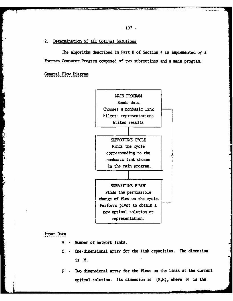
- 107 -
2. Determination of all Optimal Solutions
The algorithm described in Part B of Section 4 is implemented by a
Fortran Computer Program composed of two subroutines and a main program.
General Flow-Diagram
MAIN PROGRAM
Reads data
Chooses a nonbasic link
Filters representations
Writes results
SUBROUrINE CYCLE
Finds the cycle
corresponding to the
nonbasic link chosen
in the main program.
SUBROWrINE PIVOT
Finds the permissible
change of flow on the cycle.
Performs pivot to obtain a
new optimal solution or
representation.
M - Number of network links.
C - One-dimensional array for the link capacities. The dimension
is M.
F - Two dimensional array for the flows on the links at the current
optimal solution. Its dimension is (MN), where N is the

- 108-
estimated nu ber of different solutions and representations. A
first optimal solution must be supplied to the program (that
obtained from the maximal flow algorithm) that is F(Il).
BASE Two-dimensional array that determines which links are basic and
which nonbasic at the current solution. Its dimension is (M,N).
If link I is basic then BASE (I,,) = 1, if it is nonbasic
then BASE (I,-) - 0. The basic configuration of the first optimal
solution must be provided to the program, that is BASE(I,1).
LOUt - One-dimensional array for the exit nodes of the links.
LIN - One-dimensional array for the entrance nodes of the links.
The program writes all the extremal optimal solutions and their number.
In addition it writes the number of different solutions and representations
searched during the execution.
Dimensioned Local Variables
DIRPF, BFR and LAB are one-dimensional arrays of dimension M.

-109
C DETERMINATIONJ OF ALL 10LT1OAL -',flLUT1P'JS - '4A1N PQrRlAMTNTEGEP CCle(9i; v"~r
-REAO(5.10) h
RFA015.l 1) (CI~i~
Kal
Npa 1
I J10O2 J1ZJ1+l
IF- (4$ASF(JtI(),GT.C 1' - 2CALL CYVCL'
00) 200 J=19N
P.~00 CnNT INUEFGO TO 2
to C0 CONTI NUE
12-12+1GO TO 2
IF(1.*GE"lGO TO I
WRITEC 6.16) MRto FORt4AT(12)it P0If*AT(3bI2)
14 FORMAT(/5X*9(12%(-W)I
16 FOR?*AT(///2X9N4M.~-1-E UF DIFFCNT FMIUTIONS ANt) :;F0R-SPNTArT.O4S
GERUG SU!,CHKS tooE ND
SIM'POUT1NE. DIVOTINTFGF-P C(0)9FPe99SoCOMMON Kv, K.?90FLT*J1.11,C *LOUT(o) 9L N( 0 9F9 AIRIE91 R, ORwp.M.Na
100 F(I*KIP=V(I9K)* 12al1
I PDR(t)~.), Trl 2
GO TO 32 F(t1,KI)=F(11I*K)+DELT3 IWr(TtaEO.JI)GO TOA
GO TO II'rfFrI2,KI).e0.C('1)4',O TOI~rFft(2.K1)eEfQ.O)fO Tr) 512 .OP R f12kGO TO A
S 00 200 TzleN200 SASf41IK1JwAS~fI.KI
BASE(JI.IC1IulFJASErf29K1)*o
D~O 400 1S1.K200 3%00 j*19!m11F(J.ki)o.E.&( Jet) )fv TO 400i
IF(85F(JK1).~.~ACJ~l)~"rn Aoo300 CONTIN.UE
K ISK 1-1L400 C01T INe

110
K 5UPQU1NE CYCLF
L=OC
J2=j 100 100 11.em
100 L#A(1)wO
25 J=O1 Int2 Ir-(IGTPw)GI2 T'i
GO Tfl (10911)04111 IFfL3UT( I?*P4L*Lf'tT( j ));. M,
GO TO) 1210 19 (LOUT( I)*[email protected]))GO In .112 1F'AL1K.t.J,~TO
IP(LA8(M)eF0.1)Gl Tf) ~200 CONTINUE
DIRPI )3
GO TO (2t922).?21 IF(L1N(I)eE0*L0UT(jI))G0 TO -
GO TO 322 IF(L1N(1)*EQ.LtN4J1))GO TO P3 331+1
Go TO 2
5 IF(I*GT.w4)GO TO 76O TO (13914).141
14 !~(LJN(I).NE*LOUT(J21)GO TO S'GO TO IS
13 IW(LIN(T)eN0~LJN4JT)rO T115 IF(B3ASE(1,%.)*NF*1)G3 TO
DO 300 4=19mIft(LA8(N)wE0*I)Gqj TO 6
300 CONTINtFEOIRPCI )--I
LA9( j)wJ
GO TO (239241,942P3 ZPr(LOUT(I)*'o.L0UT(J))Gt, TO 9
Gn TO 624 I7(LOU1T.I)EQLIN(Jt)GO TM ~6 1 a +3I
6O TO 57 L4..*I
J?mLASICL)
IF (0 .5(2),rO.-I)Y 12GO TO I
GO To 16
DELT*(1 sKIIA j3w9pR(JJ
lF(0TFP(j3).F0*.)G~O TO 17I 0(OEL?*.T9FfJ3 K ) )GO TO ip,
GO TO 13M
OE-LTwC(J3)-F TO is
to CALL PIv']T
- 111 -
References
[B1] Balinski, M.L., "An Algorithm for Finding All the Vertices of Convex
Polyhedral Sets", J. Soc. Indust. Appl. Math., Vol. 9, No. 1,
March 1961.
(B2] Bloom, J., "A Program for Chernikova's Algorithm", Electronic Systems
Laboratory, M.I.T., March 1976.
[B3] Bazaraa, M.S. and Jarvis, J.J., Linear Programming and Network Flows,
John Wiley & Sons, 1977.
(Chl] Chernikova, N.V., "Algorithm for Finding a General Formula for the Non-
negative Solutions of a System of Linear Equations", U.S.S.R. Com-
putational Mathematics and Mathematical Physics, 4, pp. 151-158,
1964.
[Ch2] Chernikova, N.V., "Algorithm for Finding a General Formula for the Non-
negative Solutions of a System of Linear Inequalities", U.S.S.R.
Computational Mathematics and Mathematical Physics, 5, pp
pp. 228-233, 1965.
[El] Even, S., Algorithmic Combinatorics, The MacMillan Company, N.Y., 1973.
(Fl] Ford, L.R., Jr., and Fulkerson, D.R., 'Maximal Flow Through a Network",
Canadian J. Math., 8 (3), pp. 339-404, 1950.
[HI] Hu, T.C., Integer Programming and Network Flows, Addison-Wesley, 1970.
[LI] Luenberger, D.G., Introduction to Linear and Nonlinear Progranming,
Addison-Wesley, 1973.
[Ml] Moss, F.H., "The Application of Optimal Control Theory to Dynamic Rout-ing in Data Communication Networks", Ph.D. Dissertation, Massa-
chusetts Inst. Technol., Cambridge, 1976.
(M] Moss, F.H. and Segall, A., "An Optimal C6ntrol Approach to Dynamic
Routing in Data tcmunication Networks, Part I: Principles",
E.E. Pub. No. 312, Technion - Israel Inst. Technol., Sept. 1977.
- 112 -
[M31 Nbss, F.H. and Segall, A., "An Optimal Control Approach to Dynamic Rout-
ing in Data Commication Networks, Part II: Geometrical Interpreta-tion", E.E. Pub. No. 319. Technion - Israel Inst. Technol., Jan. 1978.
[M4] Mattheiss, T.H., "An Algorithm for Determining Irrelevant Constraintsand all the Vertices in Systems of Linear Inequalities", Oper-tions Research, Vol. 21, No. 1, 247, Jan.-Feb. 1973.
[RI] Rubin, D.C., "Vertex Generation and Cardinality Linear Programs", Operations Research, 23, pp. SSS-564, 1975.
(S1] Segall, A., '"he Modelling of Adaptive Routing in Data CommicationNetworks", IEEE Trans. on Com., CCM-2S, No. 1, pp. 85-95,January 1977.
7.-

ACKNOWLEDGEMENT
The'authors would like to thank Dr. F.H. Moss for stimulat-
ing discussions regarding the first stages of this work.