A unified deep artificial neural network approach topartial differential equations in complex geometries

Jens Berg∗ and Kaj Nystrom†

Department of Mathematics, Uppsala UniversityS-751 06 Uppsala, Sweden

Abstract

We use deep feedforward artificial neural networks to approximate solutionsof partial differential equations of advection and diffusion type in complex ge-ometries. We derive analytical expressions of the gradients of the cost functionwith respect to the network parameters, as well as the gradient of the networkitself with respect to the input, for arbitrarily deep networks. The method isbased on an ansatz for the solution, which requires nothing but feedforwardneural networks, and an unconstrained gradient based optimization methodsuch as gradient descent or quasi-Newton methods.

We provide detailed examples on how to use deep feedforward neural net-works as a basis for further work on deep neural network approximations topartial differential equations. We highlight the benefits of deep compared toshallow neural networks and other convergence enhancing techniques.

1 Introduction

Partial differential equations (PDEs) are used to model a variety of phenomena inthe natural sciences. Common to most of the PDEs encountered in practical appli-cations is that they cannot be solved analytically, but require various approximationtechniques. Traditionally, mesh based methods such as finite elements (FEM), finite

∗jens.berg@math.uu.se†kaj.nystrom@math.uu.se

1

arX

iv:1

711.

0646

4v1

[st

at.M

L]

17

Nov

201

7

differences (FDM), or finite volumes (FVM), are the dominant techniques for obtain-ing approximate solutions. These techniques require that the computational domainof interest is discretized into a set of mesh points, and the solution is approximatedat the points of the mesh. The advantage of these methods is that they are veryefficient for low-dimensional problems on regular geometries. The drawback is thatfor complicated geometries, meshing can be as difficult as the numerical solution ofthe PDE itself. Moreover, the solution is only computed in the mesh points andevaluation of the solution in any other point requires interpolation or some otherreconstruction method.

Other methods do not require a mesh but a set of collocation points where thesolution is approximated. The collocation points can be generated according to somedistribution inside the domain of interest and examples include radial basis functions(RBF) and Monte Carlo methods (MCM). The advantage is that it is relatively easyto generate collocation points inside the domain by a hit-and-miss approach. Thedrawbacks of these methods, compared to traditional mesh based methods, are forexample numerical stability for RBF and inefficiency for MCM.

The last decade has seen a revolution in deep learning, where deep artificial neu-ral networks (ANNs) are the key component. ANNs is not a new concept. They havebeen around since the 40’s [25] and used for various applications. A historical review,in particular in the context of differential equations can be found in ch. 2 of [36]. Thesuccess of deep learning during the last decade is due to a combination of improvedtheory, starting with unsupervised pre-training and deep belief nets, and improvedhardware resources such as general purpose graphics processing units (GPGPUs).See for example [11, 20]. Deep ANNs are now routinely used with impressive resultsin areas ranging from image analysis, pattern recognition, object detection, natu-ral language processing, to self-driving cars. Simple feedforward ANNs have not yetenjoyed the same success as recurrent ANNs, for natural language processing, or con-volutional ANNs, for image analysis. However, recent results show that feedforwardANNs have great potential by allowing self-normalizing activation functions [18].

While deep ANNs have achieved impressive results in several important appli-cation, there are still many open questions concerning how and why they actuallywork so efficiently. From the perspective of function approximation theory it hasbeen known since the 90’s that ANNs are universal approximators that can be usedto approximate any continuous function and its derivatives [12, 13, 5, 24]. In thecontext of PDEs, single hidden layer ANNs have traditionally been used to solvePDEs since one hidden layer with sufficiently many neurons is sufficient for approxi-mating any function, and all gradients that are needed can be computed in analyticalclosed form [22, 23, 26]. More recently, there is a limited but emerging literature on

2

the use of deep ANNs to solve PDEs [31, 30, 6, 3]. For an overview of some of thedevelopments we refer the reader to [21]. In general ANNs have the benefits thatthey are smooth, analytical functions which can be evaluated at any point inside, oreven outside, the domain without reconstruction.

The aim of this paper is twofold. The first is to introduce a unified methodof solving PDEs which only involves feedforward deep ANNs with (close to) nouser intervention. In previous works, see for example Lagaris et. al. [22], onlya single hidden layer is used, and the method outlined requires some user-definedfunctions which are non-trivial, or even impossible, to compute. Later, Lagaris et.al [23] removed the need for user intervention by using a combination of feedforwardand radial basis function ANNs in a non-trivial way. Later work by McFall andMahan [26] removed the need for the radial basis function ANN by replacing it withlength factors that are computed using thin plate splines. The thin plate splinescomputation is, however, rather cumbersome as it involves the solution of manylinear systems which adds extra complexity to the problem. In contrast, the methodproposed in this paper requires only an implementation of a deep feedforward ANNtogether with a cost function and any choice of unconstrained numerical optimizationmethod. We derive analytical expressions for the gradient of the cost function withrespect to the network parameters, together with the gradients of the network withrespect to the input, for arbitrarily deep networks. This is the focus in the first partof the paper.

The second aim is to propose PDEs as a vehicle for further theoretical explorationsof deep ANNs. Most applications of deep ANNs, in for example image analysis oraudio processing, are too complicated to be used as analytical tools. In contrast,with PDEs we can have complete understanding of the input-output relations andwe can study the training process for various ANN configurations. This is the focusin the second part of the paper. In this context we recall that a general problem indeep learning is to find a sufficient amount of labeled data to use in training. Whilethis is becoming less and less of a problem due to the community’s effort to produceopen datasets, we simply note that by using the PDE itself we can generate as muchdata as needed.

The rest of the paper is organized as follows. In section 2 we recall the net-work architecture of deep, fully connected feedforward ANNs, we introduce somenecessary notation and the backpropagation scheme. In section 3 we develop unifiedartificial neural network approximations for stationary PDEs. Based on our ansatzfor the solution we discuss extension of the boundary data, smooth distance functionapproximation and computation, gradient computations and the backpropagationalgorithm for parameter calibration. We give detailed account of the latter compu-

3

tations/algorithms in the case of advection and diffusion problems. In section 4 weprovide some concrete examples concerning how to apply the method outlined. Ourexamples include linear advection and diffusion in 1D and 2D, but high-dimensionalproblems are also discussed. Section 5 is devoted to convergence considerations. Astraining neural networks consumes a lot of time and computational resources, it isdesirable to reduce the number of required iterations until a certain accuracy hasbeen reached. During this work, we have found two factors which strongly influencethe number of required iterations in our PDE focused applications/examples. Thefirst is pre-training the network using the available boundary data, and the secondis to increase the number of hidden layers. In section 5 we discuss this in more de-tail and one particular finding is that we, by fixing the capacity of the network andincreasing the number of hidden layers, can see a dramatic decrease in the numberof iterations required to reach a desired level of accuracy. Our findings indicate thatusing deep ANNs instead of just shallow ones adds real value in the context of usingANNs to solve PDEs. Finally, section 6 is devoted to a summary, conclusions andan outlook on future work.

2 Network architecture

In this paper, we consider deep, fully connected feedforward ANNs. The ANN con-sists of L+ 1 layers, where layer 0 is the input layer and layer L is the output layer.The layers 0 < l < L are the hidden layers. The activation functions in the hiddenlayers can be any activation function such as for example sigmoids, rectified linearunits, or hyperbolic tangents. Unless otherwise stated, we will use sigmoids in thehidden layers. The output activation will be the linear activation. The ANN definesa mapping RN → RM .

Each neuron in the ANN is supplied with a bias, including the output neuronsbut excluding the input neurons, and the connections between neurons in subsequentlayers are represented by matrices of weights. We let blj denote the bias of neuronj in layer l. The weight between neuron k in layer l − 1, and neuron j in layer l isdenoted by wl

jk. The activation function in layer l will be denoted by σl regardlessof the type of activation. We assume for simplicity that a single activation functionis used for each layer. The output from neuron j in layer l will be denoted by ylj.See Figure 1 for a schematic representation of a fully connected feedforward ANN.

A quantity that will be extensively used is the so-called weighted input which isdefined as

zlj =∑k

wljkσl−1(zl−1

k ) + blj, (2.1)

4

...

...

bl−1k

...

...blj

...

...

x1

xN

bL1

bLM

yL1

yLM

wljk

Layer 0 Layer l − 1 Layer l Layer L

Figure 1: Schematic representation of a fully connected feedforward ANN.

where the sum is taken over all inputs to neuron j in layer l. That is, the numberof neurons in layer l − 1. The weighted input (2.1) can of course also be written interms of the output from the previous layer as

zlj =∑k

wljky

l−1k + blj, (2.2)

where the output yl−1k = σl−1(zl−1

k ) is the activation of the weighted input. As wewill be working with deep ANNs, we will prefer formula (2.1) as it naturally definesa recursion in terms of previous weighted inputs through the ANN. By definition wehave

σ0(z0j ) = y0

j = xj, (2.3)

which terminates any recursion.By dropping the subscripts we can write (2.1) in the convenient vectorial form

zl = W lσl−1(zl−1) + bl = W lyl−1 + bl, (2.4)

where each element in the zl and yl vectors are given by zlj and ylj, respectively, andthe activation function is applied elementwise. The elements of the matrix W l aregiven by W l

jk = wljk.

With the above definitions, the feedforward algorithm for computing the output

5

yL, given the input x, is given by

yL = σL(zL)

zL = WLσL−1(zL−1) + bL

zL−1 = WL−1σL−2(zL−2) + bL−1

...

z2 = W 2σ1(z1) + b2

z1 = W 1x+ b1.

(2.5)

2.1 Backpropagation

Given some data x = [x1, . . . , xN ]T ∈ RN and some target outputs y = [y1, . . . , yM ]T ∈RM we wish to choose our weights and biases such that yL(x;w, b) is a good approx-imation of y(x). We use the notation yL(x;w, b) to indicate that the ANN takes xas input and that the ANN is parametrized by the weights and biases, w, b. To findthe weights and biases, we define some cost function C = C(y, yL) : RN → R andcompute

w∗, b∗ = arg minw,b

C(y, yL). (2.6)

The minimization problem (2.6) can be solved using a variety of optimization meth-ods, both gradient based and gradient free. In this paper, we will focus on gradientbased methods and derive the gradients that we need in order to use any gradientbased optimization method. The standard way of computing gradients is by usingbackpropagation. The main ingredient is the error of neuron j in layer l defined by

δlj =∂C

∂zlj. (2.7)

The standard backpropagation algorithm for computing the gradients of the costfunction is then given by

δLj =∂C

∂yLjσ′L(zLj ),

∂C

∂wljk

= yl−1k δlj,

δlj =∑k

wl+1kj δ

l+1k σ′l(z

lj),

∂C

∂blj= δlj.

(2.8)

The δ-terms in (2.8) can be written in vectorial form as

δL = ∇yLC σ′L(zL), δl = (W l+1)T δl+1 σ′l(zl), (2.9)

6

where we use the notation ∇yLC = [ ∂C∂yL1

, . . . , ∂C∂yLM

]T , and denotes the Hadamard,

or componentwise, product. The notation ∇C, without a subscript, will denote thevector of partial derivatives with respect to the inputs, x. Note the transpose onthe weight matrix W . The transpose W T is the Jacobian matrix of the coordinatetransformation between layer l + 1 and l.

3 Unified ANN approximations to PDEs

In this section we interested in solving stationary PDEs of the form

Lu = f, x ∈ Ω,

Bu = g, x ∈ Γ ⊂ ∂Ω,(3.1)

where L is a differential operator, f a forcing function, B a boundary operator, andg the boundary data. The domain of interest is Ω ⊂ RN , ∂Ω denotes its boundary,and Γ is the part of the boundary where boundary conditions should be imposed. Inthis paper, we focus on problems where L is either the advection or diffusion oper-ator, or some mix thereof. The extension to higher order problems are conceptuallystraightforward based on the derivations outlined below.

We consider the ansatz u = u(x;w, b) for u where (w, b) denotes the parametersof the underlying ANN. To determine the parameters we will use the cost functiondefined as the quadratic residual,

C =1

2||Lu− f ||2 :=

1

2

∫Ω

|Lu− f |2 dx. (3.2)

For further reference we need the gradient of (3.2) with respect to any networkparameter. Let p denote any of wl

jk or blj. Then

∂C

∂p= (Lu− f) (L

∂u

∂p). (3.3)

We will use the collocation method [22] and therefore we discretize Ω and Γ intoa sets of collocation points Ωd and Γd, with |Ωd| = Nd and |Γd| = Nb, respectively.In its discrete form the minimization problem (2.6) then becomes

w∗, b∗ = arg minw,b

∑xi∈Ωd

1

2

1

Nd

||Lu(xi)− f(xi)||2, (3.4)

7

subject to the constraints

Bu(xi) = g(xi), ∀xi ∈ Γd. (3.5)

There are many approaches to the minimization problem (3.4) subject to theconstraints (3.5). One can for example use a constraint optimization procedure,Lagrange multipliers, or penalty formulations to include the constraints in the op-timization. Another approach is to design the ansatz u, such that the constraintsare automatically fulfilled, thus turning the constrained optimization problem intoan unconstrained optimization problem. Unconstrained optimization problems canbe more efficiently solved using gradient based optimization techniques.

In the following, we let, for simplicity, B in (3.1) be the identity operator, andwe hence consider PDEs with Dirichlet boundary conditions. The specific ansatz forthe solution we consider in the following is

u(x) = G(x) +D(x)yL(x;w, b), (3.6)

where G = G(x) is a smooth extension of the boundary data g and D = D(x)is a smooth distance function giving the distance for x ∈ Ω to Γ. Note that theform of the ansatz (3.6) ensures that u attains its boundary values at the boundarypoints. Moreover, G and D are pre-computed using low-capacity ANNs for the givenboundary data and geometry using only a small subset of the collocation points,and do not add any extra complexity when minimizing (3.4). We call this approachunified as there are no other ingredients involved other than feedforward ANNs, andgradient based, unconstrained optimization methods to compute all of G, D, and yL.

3.1 Extension of the boundary data

The ansatz (3.6) requires that G is globally defined, smooth1, and that

|G(x)− g(x)| < ε, ∀x ∈ Γ. (3.7)

Other than these requirements, the exact form of G is not important. It is hence anideal candidate for an ANN approximation. To compute G, we simply train an ANNto fit g(x), ∀x ∈ Γd. The quadratic cost function used is given by

C =1

2

1

Nb

∑xi∈Γd

||G(xi)− g(xi)||2, (3.8)

1It is sufficient that G has continuous derivatives up to the order of the differential operator L.However, since G will be computed using an ANN, it will be smooth.

8

and in the course of calibration we compute the gradients using the standard back-propagation (2.8). Note that in general we have Nb << Nd and the time it takes tocompute G is of lower order.

3.2 Smooth distance function computation

To compute the smooth distance function D, we start by computing a non-smoothdistance function, d, and approximate it using a low-capacity ANN. For each point,x, we define d as the minimum distance to a boundary point where a boundarycondition should be imposed. That is,

d(x) = minxb∈Γ||x− xb||. (3.9)

Again, the exact form of d (and D) is not important other than that D is smoothand

|D(x)| < ε, ∀x ∈ Γ. (3.10)

We can use a small subset ωd ⊂ Ωd, with |ωd| = nd << Nd to compute d.Once d has been computed and normalized, we fit another ANN and train it using

the cost function

C =1

2

1

nd +Nb

∑xi∈ωd∪Γd

||D(xi)− d(xi)||2. (3.11)

Note that we train the ANN over the points xi ∈ ωd ∪ Γd, with d(xi) = 0 ∀xi ∈ Γd.Since the ANN defining the smooth distance function can be taken to be a singlehidden layer, low-capacity ANN with nd + Nb << Nd, the total time to computeboth d and D is of lower order. See Figure 2 for (rather trivial examples) of d andD in one dimension.

Remark 3.1. We stress that the distance function (3.9) can be computed efficientlywith nearest-neighbor searches, using for example k-d trees [1], or ball trees [29]for very high-dimensional input. A naıve nearest neighbor search will have O(NdNb)complexity, while an efficient nearest-neighbor search will typically haveO(Nd logNb).

Remark 3.2. Instead of computing the actual distance function, we could use themore extreme version

d(x) =

0, x ∈ Γ,

1, otherwise.(3.12)

However, simulations showed that this function and its approximating ANN have anegative impact on convergence and quality when computing u.

9

0.0 0.2 0.4 0.6 0.8 1.0x

0.0

0.2

0.4

0.6

0.8

1.0 Distance functionNetwork smoothing

(a) L = d/dx. Only one boundary conditionat x = 0.

0.0 0.2 0.4 0.6 0.8 1.0x

0.0

0.2

0.4

0.6

0.8

1.0

Distance functionNetwork smoothing

(b) L = d2/dx2. Boundary conditions atboth boundary points.

Figure 2: Smoothed distance functions using single hidden layer ANNs with 5 hiddenneurons, using 100 collocation points.

3.3 Gradient computations

When the differential operator L acts on the ansatz u in (3.6), we need, as Ω ⊂ RN ,to compute the partial derivatives of the ANNs with respect to the spatial variables(x1, ..., xN). Also, when using gradient based optimization we need to compute thegradients of the quadratic residual cost function (3.2), and also the ANNs, withrespect to the network parameters.

In the single hidden layer case, all gradients can be computed in closed analyticalform as shown in [22]. For deep ANNs, however, we need to modify the feedforward(2.5) and backpropagation (2.8) algorithms to compute the gradients with respectto (x1, ..., xN) and network parameters, respectively.

Note that the minimization problem in (3.4) involves the collocation points xi.In the following, and throughout the paper, we will, with a slight abuse of notation,by ∂

∂xialways denote the derivative with respect to the spatial coordinate xi, not

with respect to collocation point xi.

3.3.1 Advection problems

For advection problems we have a PDE of the form

Lu = ∇ · (V u) = f, (3.13)

10

for some (non-linear) matrix coefficient V . When the advection operator L acts on uwe need to compute the gradient of the ANN with respect to the input. The gradientscan be computed by taking partial derivatives of (2.5). We get, in component form,

∂yLj∂xi

= σ′(zLj )∂zLj∂xi

∂zLj∂xi

=∑k

wLjkσ′L−1(zL−1

k )∂zL−1

k

∂xi

∂zL−1j

∂xi=∑k

wL−1jk σ′L−2(zL−2

k )∂zL−2

k

∂xi

...

∂z2j

∂xi=∑k

w2jkσ′1(z1

k)∂z1

k

∂xi

∂z1j

∂xi= w1

ji.

(3.14)

Note the slight abuse of subscript notation in order to avoid having too many sub-scripts. Note also that (3.14) defines a new ANN with the same weights, but nobiases, as the original ANN with modified activation functions. A convenient vecto-rial form is obtained by dropping the subscripts and re-writing (3.14) as

∂yL

∂xi= σ′L(zL) ∂zL

∂xi∂zL

∂xi= WLσ′L−1(zL−1) ∂zL−1

∂xi∂zL−1

∂xi= WL−1σ′L−2(zL−2) ∂zL−2

∂xi...

∂z2

∂xi= W 2σ′1(z1) ∂z1

∂xi∂z1

∂xi= W 1ei,

(3.15)

where ei is the ith standard basis vector. To compute all gradients simultaneously,we define, for a vector v and vector-valued function f , the diagonal and Jacobian

11

matrices

Σ(v) =

v1 0 · · · 00 v2 · · · 0...

.... . .

...0 0 · · · vN

, J(f) =

∂f1∂x1

∂f1∂x2

· · · ∂f1∂xN

∂f2∂x1

∂f2∂x2

· · · ∂f2∂xN

......

......

∂fM−1

∂x1· · · ∂fM−1

∂xN−1

∂fM−1

∂xN∂fM∂x1

· · · ∂fM∂xN−1

∂fM∂xN

. (3.16)

Using these matrices, we can write all partial derivatives in the compact matrix form

J(yL) = Σ(σ′L(zL))J(zL)

J(zL) = WLΣ(σ′L−1(zL−1))J(zL−1)

J(zL−1) = WL−1Σ(σ′L−2(zL−2))J(zL−2)

...

J(z2) = W 2Σ(σ′1(z1))J(z1)

J(z1) = W 1IN×N ,

(3.17)

where IN×N is the N ×N identity matrix. All gradients of the ANN with respect tothe input are contained in the rows of the Jacobian matrix J(yL) as

J(yL) =

· · · (∇yL1 )T · · ·· · · ... · · ·· · · (∇yLM)T · · ·

. (3.18)

To solve the PDE (3.13), we need to modify the backpropagation algorithm (2.8)to include the gradients of the residual cost function (3.2) with respect to the networkparameters. First, we need to compute

∂yLm∂wl

jk

,∂yLm∂blj

, m = 1, . . . ,M. (3.19)

This can be done componentwise by using backpropagation with the identity as thecost function. That is, we let C(yLm) = yLm and then (2.8) becomes

δLm = σ′L(zLm),∂yLm∂wl

jk

= yl−1k δlj,

δlj =∑k

wl+1kj δ

l+1k σ′l(z

lj),

∂yLm∂blj

= δlj.

(3.20)

12

The δ-terms in (3.20) can be written in vectorial form as

δL = σ′L(zL),

δl = (W l+1)T δl+1 σ′l(zl).(3.21)

Secondly, we need to compute

∂2yLm∂xi∂wl

jk

,∂2yLm∂xi∂blj

, i = 1, . . . , N, m = 1, . . . ,M. (3.22)

This can be done by taking the partial derivative of (3.20) with respect to xi. Weget

δLm∂xi

= σ′′L(zLm)∂zLm∂xi

,

∂δlj∂xi

=∑k

wl+1kj

(∂δl+1

k

∂xiσ′l(z

lj) + δl+1

k σ′′l (zlj)∂zlj∂xi

),

∂2yLm∂xi∂wl

jk

=∂yl−1

k

∂xiδlj + yl−1

k

∂δlj∂xi

,

∂2yLm∂xi∂blj

=∂δlj∂xi

.

(3.23)

The δ-terms in (3.23) can again be written in vectorial form as

δL

∂xi= σ′′L(zL) ∂zL

∂xi,

∂δl

∂xi= (W l+1)T

(∂δl+1

∂xi σ′l(zl) + δl+1 σ′′l (zl) ∂zl

∂xi

),

(3.24)

or in matrix form as

J(δL) = Σ(σ′′L(zL))J(zL),

J(δl) = (W l+1)T(Σ(σ′l(z

l))J(δl+1) + Σ(σ′′l (zl))Σ(δl+1)J(zl)).

(3.25)

The feedforward and backpropagation algorithms (2.5), (3.14), (3.20), and (3.23),are sufficient to compute the solution to any first-order PDE, both linear and non-linear.

Remark 3.3. Note that all data from a standard feedforward and backpropagationpass is re-used in the computation of (3.14) and (3.23). The complexity of computing(3.14) and (3.23) is thus the same as when computing (2.5) and (2.8), with someadditional memory overhead to store the activations and weighted inputs.

13

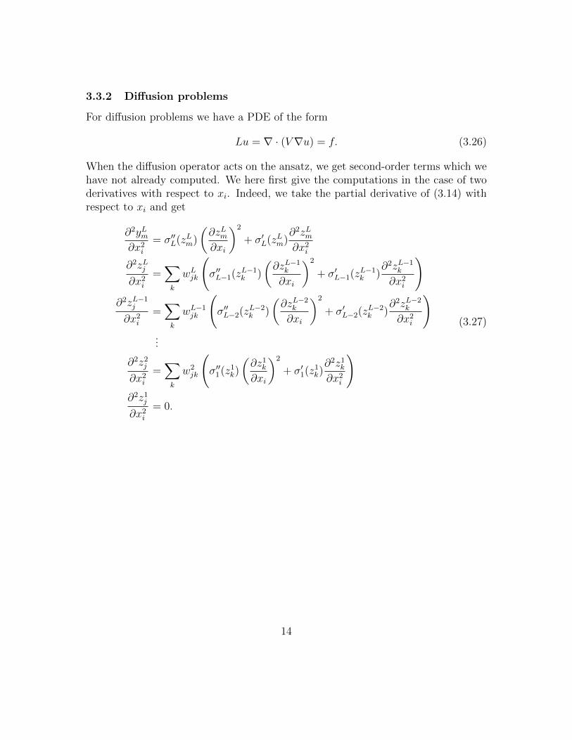
3.3.2 Diffusion problems

For diffusion problems we have a PDE of the form

Lu = ∇ · (V∇u) = f. (3.26)

When the diffusion operator acts on the ansatz, we get second-order terms which wehave not already computed. We here first give the computations in the case of twoderivatives with respect to xi. Indeed, we take the partial derivative of (3.14) withrespect to xi and get

∂2yLm∂x2

i

= σ′′L(zLm)

(∂zLm∂xi

)2

+ σ′L(zLm)∂2zLm∂x2

i

∂2zLj∂x2

i

=∑k

wLjk

(σ′′L−1(zL−1

k )

(∂zL−1

k

∂xi

)2

+ σ′L−1(zL−1k )

∂2zL−1k

∂x2i

)∂2zL−1

j

∂x2i

=∑k

wL−1jk

(σ′′L−2(zL−2

k )

(∂zL−2

k

∂xi

)2

+ σ′L−2(zL−2k )

∂2zL−2k

∂x2i

)...

∂2z2j

∂x2i

=∑k

w2jk

(σ′′1(z1

k)

(∂z1

k

∂xi

)2

+ σ′1(z1k)∂2z1

k

∂x2i

)∂2z1

j

∂x2i

= 0.

(3.27)

14

The vectorial form of (3.27) can be written as

∂2yL

∂x2i

= σ′′L(zL)

(∂zL

∂xi

)2

+ σ′L(zL)∂2zL

∂x2i

∂2zL

∂x2i

= WL

(σ′′L−1(zL−1)

(∂zL−1

∂xi

)2

+ σ′L−1(zL−1) ∂2zL−1

∂x2i

)∂2zL−1

∂x2i

= WL−1

(σ′′L−2(zL−2)

(∂zL−2

∂xi

)2

+ σ′L−2(zL−2) ∂2zL−2

∂x2i

)...

∂2z2

∂x2i

= W 2

(σ′′1(z1)

(∂z1

∂xi

)2

+ σ′1(z1) ∂2z1

∂x2i

)∂2z1

∂x2i

= 0N ,

(3.28)

where 0N = [0, . . . , 0]T denotes the zero vector with N elements. To write thematrix form of (3.27) we define J2(f) to be the matrix of non-mixed second partialderivatives of a vector-valued function f ,

J2(f) =

∂2f1∂x2

1

∂2f1∂x2

2· · · ∂2f1

∂x2N

∂2f2∂x2

1

∂2f2∂x2

2· · · ∂2f2

∂x2N

......

......

∂2f2M−1

∂x1· · · ∂2fM−1

∂x2N−1

∂2fM−1

∂x2N

∂2fM∂x2

1· · · ∂2fM

∂x2N−1

∂2fM∂x2

N

. (3.29)

The matrix form can then be written as

J2(yL) = Σ(σ′′(zL))J(zL)2 + Σ(σ′L(zL))J2(zL)

J2(zL) = WL(Σ(σ′′L−1(zL−1))J(zL−1)2 + Σ(σ′L−1(zL−1))J2(zL−1))

J2(zL−1) = WL−1(Σ(σ′′L−2(zL−2))J(zL−2)2 + Σ(σ′L−2(zL−2))J2(zL−2))

...

J2(z2) = W 2(Σ(σ′′1(z1))J(z1)2 + Σ(σ′1(z1))J2(z1))

J2(z1) = W 1ZN×N ,

(3.30)

where ZN×N is the zero matrix of dimension N ×N .

15

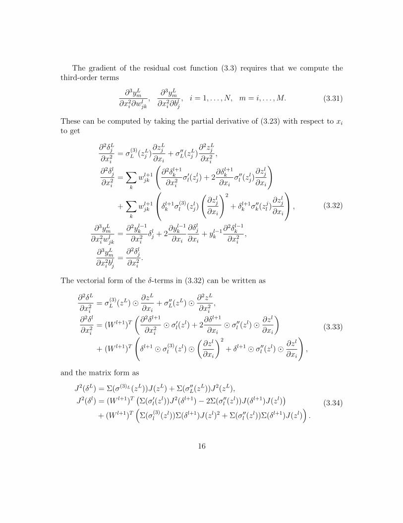
The gradient of the residual cost function (3.3) requires that we compute thethird-order terms

∂3yLm∂x2

i∂wljk

,∂3yLm∂x2

i∂blj

, i = 1, . . . , N, m = i, . . . ,M. (3.31)

These can be computed by taking the partial derivative of (3.23) with respect to xito get

∂2δLj∂x2

i

= σ(3)L (zLj )

∂zLj∂xi

+ σ′′L(zLj )∂2zLj∂x2

i

,

∂2δlj∂x2

i

=∑k

wl+1jk

(∂2δl+1

k

∂x2i

σ′l(zlj) + 2

∂δl+1k

∂xiσ′′l (zlj)

∂zlj∂xi

)

+∑k

wl+1jk

δl+1k σ

(3)l (zlj)

(∂zlj∂xi

)2

+ δl+1k σ′′k(zjl )

∂zlj∂xi

,

∂3yLm∂x2

iwljk

=∂2yl−1

k

∂x2i

δlj + 2∂yl−1

k

∂xi

∂δlj∂xi

+ yl−1k

∂2δl−1k

∂x2i

,

∂3yLm∂x2

i blj

=∂2δlj∂x2

i

.

(3.32)

The vectorial form of the δ-terms in (3.32) can be written as

∂2δL

∂x2i

= σ(3)L (zL) ∂zL

∂xi+ σ′′L(zL) ∂2zL

∂x2i

,

∂2δl

∂x2i

= (W l+1)T(∂2δl+1

∂x2i

σ′l(zl) + 2∂δl+1

∂xi σ′′l (zl) ∂zl

∂xi

)+ (W l+1)T

(δl+1 σ(3)

l (zl)(∂zl

∂xi

)2

+ δl+1 σ′′l (zl) ∂zl

∂xi

),

(3.33)

and the matrix form as

J2(δL) = Σ(σ(3)L(zL))J(zL) + Σ(σ′′L(zL))J2(zL),

J2(δl) = (W l+1)T(Σ(σ′l(z

l))J2(δl+1)− 2Σ(σ′′l (zl))J(δl+1)J(zl))

+ (W l+1)T(

Σ(σ(3)l (zl))Σ(δl+1)J(zl)2 + Σ(σ′′l (zl))Σ(δl+1)J(zl)

).

(3.34)

16

The feedforward and backpropagation algorithms (2.5), (3.14), (3.20), (3.23),(3.27), and (3.32) can be used to solve any second-order PDE, both linear and non-linear. To compute mixed derivatives, (3.27) and (3.32) have to be modified bytaking the appropriate partial derivative of (3.14), and (3.23). Higher-order PDEscan be solved by repeated differentiation of the feedforward and backpropagationalgorithms. Note that to compute second-order derivatives, the weighted inputs,partial derivatives of the weighted inputs, activations, and partial derivatives of theactivations needs to be re-computed or stored from the previous forward and back-ward passes.

4 Numerical examples

In this section we provide some concrete examples concerning how to apply themodified feedforward and backpropagation algorithms to model problems. Eachproblem requires their own modified backpropagation algorithms depending on thedifferential operator L. We start by some simple examples in some detail and latershow some examples of more complicated problems.

In all the following numerical examples we have implemented the gradients ac-cording to the schemes presented in the previous section, and we consequently usethe BFGS [7] method, with default settings, from SciPy [17] to train the ANN. Wehave tried all gradient free and gradient based numerical optimization methods avail-able in the scipy.optimize package, and the online, batch, and stochastic gradientdescent methods. BFGS shows superior performance compared to all other methodswe have tried.

An issue one might encounter is that the line search in BFGS fails due to theHessian matrix being very ill-conditioned. To circumvent this, we use a BFGS incombination with stochastic gradient descent. When BFGS fails due to line searchfailure, we run 1000 iterations with stochastic gradient descent with a very smalllearning rate, in the order of 10−9, to bring BFGS out of the troublesome region. Thisprocedure is repeated until convergence, or until the maximum number of allowediterations has been exceeded.

4.1 Linear advection in 1D

The stationary, scalar, linear advection equation in 1D is given by

Lu =du

dx= f, 0 < x ≤ 1,

u(0) = g0.(4.1)

17

To get an analytic solution we take, for example,

u = sin(2πx) cos(4πx) + 1, (4.2)

and plug it into (4.1) to compute f and g0. In this simple case, the boundary dataextension can be taken as the constant G(x) ≡ u(0) = 1 and the smoothed distancefunction can be seen in Figure 2a. In this simple case, we could take the distancefunction to be the line D(x) = x. When L acts on the ansatz u we get

Lu =dG

dx+dD

dxyL1 +D

∂yL1∂x

. (4.3)

To use a gradient based optimization method we need the gradients of the quadraticresidual cost function (3.2). They can be computed from (3.3) as

∂C

∂wljk

= (Lu− f)

(dD

dx

∂yL1∂wl

jk

+D∂2yl1

∂x∂wljk

),

∂C

∂blj= (Lu− f)

(dD

dx

∂yL1∂blj

+D∂2yl1∂x∂blj

).

(4.4)

Each of the terms in (4.3) and (4.4) can be computed using the algorithms (2.5),(2.8), (3.14), (3.20), or (3.23). The result is shown in Figure 3. In this case, we usedan ANN with 2 hidden layers, each with 10 neurons, and 100 collocation points.

0.0 0.2 0.4 0.6 0.8 1.0x

0.00

0.25

0.50

0.75

1.00

1.25

1.50

1.75

2.00

Solution

Network solutionExact solution

(a) Exact and approximate ANN solution tothe 1D stationary advection equation.

0.0 0.2 0.4 0.6 0.8 1.0x

-3.15e-05

-3.10e-05

-3.05e-05

-3.00e-05

-2.95e-05

-2.90e-05

-2.85e-05

Error

(b) The difference between the exact and ap-proximated solution.

Figure 3: Approximate solution and error. The solution is computed using 100equidistant points, using an ANN with 2 hidden layers with 10 neurons each.

18

4.2 Linear diffusion in 1D

The stationary, scalar, linear diffusion equation in 1D is given by

Lu =d2u

dx2= f, 0 < x < 1,

u(0) = g0, u(1) = g1.(4.5)

To get an analytical solution we let, for example,

u = sin(πx

2) cos(2πx) + 1, (4.6)

and compute f , g0, and g1. In this simple case, the boundary data extension can betaken as the straight line G(x) = x + 1. The smoothed distance function D is seenin Figure 2b. Here, we could instead take the smoothed distance function to be theparabola D(x) = x(1− x). When L acts on the ansatz we get

Lu =d2G

dx2+d2D

dx2yL1 + 2

dD

dx

∂yL1∂x

+D∂2yL1∂x2

, (4.7)

and to use gradient based optimization we compute (3.3) as

∂C

∂wljk

= (Lu− f)

(d2D

dx2

∂yL1∂wl

jk

+ 2dD

dx

∂2yL1∂x∂wl

jk

+D∂3yL1

∂x2∂wljk

),

∂C

∂blj= (Lu− f)

(d2D

dx2

∂yL1∂blj

+ 2dD

dx

∂2yL1∂x∂blj

+D∂3yL1∂x2∂blj

).

(4.8)

Each of the terms in (4.7) and (4.8) can be computed using the algorithms (2.5),(3.14), (3.20), (3.23), (3.27), and (3.32). The solution is shown in Figure 4, againusing an ANN with two hidden layers with 10 neurons each, and 100 collocationpoints.

19

0.0 0.2 0.4 0.6 0.8 1.0x

0.25

0.50

0.75

1.00

1.25

1.50

1.75

2.00

Solution

Network solutionExact solution

(a) Exact and approximate ANN solution tothe 1D stationary diffusion equation.

0.0 0.2 0.4 0.6 0.8 1.0x

-2.00e-03

-1.00e-03

0.00e+00

1.00e-03

2.00e-03

Error

(b) The difference between the exact and ap-proximated solution.

Figure 4: Approximate solution and error. The solution is computed using 100equidistant points, using an ANN with two hidden layers with 10 neurons each.

4.3 A remark on 1D problems

First- and second order problems in 1D have a rather interesting property — theboundary data can be added in a pure post processing step. A first order problem in1D requires only one boundary condition, and the boundary data extension can betaken as a constant. When the first-order operator acts on the ansatz, the boundarydata extension vanishes and is not used in any subsequent training. A second orderproblem in 1D requires boundary data at both boundary points, and the boundarydata extension can be taken as the line passing through these points. When thesecond-order operator acts on the ansatz, the boundary data extension vanishes andis not used in any subsequent training. For one dimensional problems we hence letthe ansatz be given by

u(x) = D(x)yL(x), (4.9)

and we can then evaluate the solution for any boundary data using

u(x) = G(x) + u(x), (4.10)

without any re-training. Even 1D equations can be time consuming for complicatedproblems and large networks, and being able to experiment with different boundarydata without any re-training is an improvement.

20

4.4 Linear advection in 2D

The stationary, scalar, linear advection equation in 2D is given by

Lu = a∂u

∂x+ b

∂u

∂y= f, x ∈ Ω,

u = g, x ∈ Γ,

(4.11)

where a, b are the (constant) advection coefficients. The set Γ ⊂ ∂Ω is the part ofthe boundary where boundary conditions should be imposed. Let n = n(x) denotethe outer unit normal to ∂Ω at x ∈ ∂Ω. Following [19], we have

Γ = x ∈ ∂Ω : (a, b) · n(x) < 0. (4.12)

The condition (4.12), usually called the inflow condition, is easily incorporated intothe computation of the distance function. Whenever we generate a boundary pointto use in the computation of the distance function, we check if (4.12) holds, and if itdoes not, we add the point to the set of collocation points.

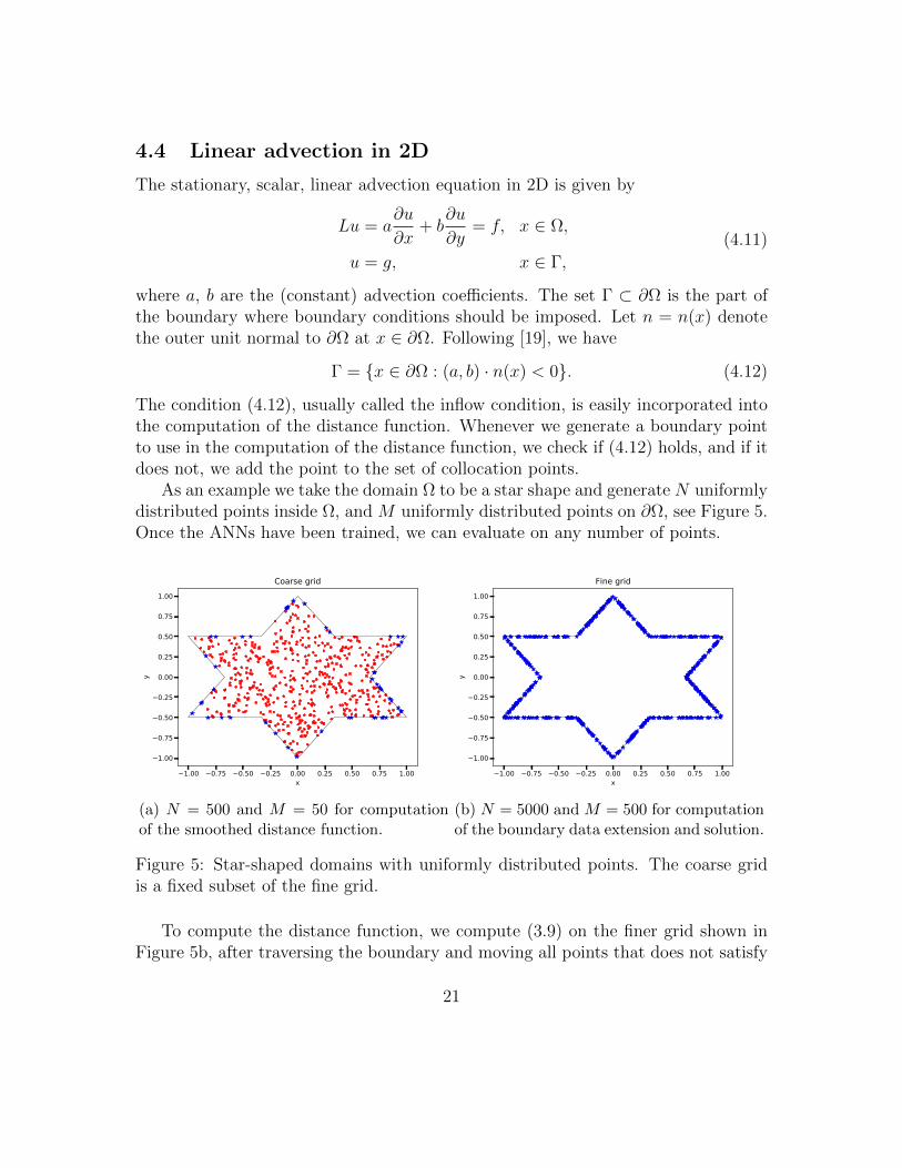
As an example we take the domain Ω to be a star shape and generate N uniformlydistributed points inside Ω, and M uniformly distributed points on ∂Ω, see Figure 5.Once the ANNs have been trained, we can evaluate on any number of points.

1.00 0.75 0.50 0.25 0.00 0.25 0.50 0.75 1.00x

1.00

0.75

0.50

0.25

0.00

0.25

0.50

0.75

1.00

y

Coarse grid

(a) N = 500 and M = 50 for computationof the smoothed distance function.

1.00 0.75 0.50 0.25 0.00 0.25 0.50 0.75 1.00x

1.00

0.75

0.50

0.25

0.00

0.25

0.50

0.75

1.00

y

Fine grid

(b) N = 5000 and M = 500 for computationof the boundary data extension and solution.

Figure 5: Star-shaped domains with uniformly distributed points. The coarse gridis a fixed subset of the fine grid.

To compute the distance function, we compute (3.9) on the finer grid shown inFigure 5b, after traversing the boundary and moving all points that does not satisfy

21

(4.12) to the set of collocation points. To compute the smoothed distance functionwe train an ANN on the coarser grid shown in Figure 5a, and evaluate it on the finergrid. The results can be seen in Figure 6.

1.00 0.75 0.50 0.25 0.00 0.25 0.50 0.75 1.00x

1.00

0.75

0.50

0.25

0.00

0.25

0.50

0.75

1.00

y

Inflow and collocation points

(a) Collocations and boundary points satis-fying the inflow condition used to computed(x).

1.00 0.75 0.50 0.25 0.00 0.25 0.50 0.75 1.00x

1.00

0.75

0.50

0.25

0.00

0.25

0.50

0.75

1.00

y

Smoothed distance function

0.0044

0.1089

0.2134

0.3180

0.4225

0.5270

0.6315

0.7360

0.8405

0.9450

(b) Smoothed distance function, D(x), com-puted on the coarse grid, using a single hid-den layer with 20 neurons.

Figure 6: Inflow points and smoothed distance function for the advection equationin 2D, with advection coefficients a = 1 and b = 1/2.

When the advection operator L acts on the ansatz we get

Lu = a

(∂G

∂x+∂D

∂xyL1 +D

∂yL1∂x

)+ b

(∂G

∂y+∂D

∂yyL1 +D

∂yL1∂y

). (4.13)

To compute the solution we need the gradients of the residual cost function, givenhere by

∂C

∂wlij

= (Lu− f)

(a

(∂D

∂x

∂yL1∂wl

ij

+D∂2yL1∂x∂wl

ij

)+ b

(∂D

∂y

∂yL1∂wl

ij

+D∂2yL1∂y∂wl

ij

)),

∂C

∂blj= (Lu− f)

(a

(∂D

∂x

∂yL1∂blj

+D∂2yL1∂x∂blj

)+ b

(∂D

∂y

∂yL1∂blj

+D∂2yL1∂y∂blj

)).

(4.14)Each of the terms in (4.13) and (4.14) can be computed using the algorithms (2.5),(2.8), (3.14), (3.20), or (3.23) as before. Note that the full gradient vectors can becomputed simultaneously, and there is no need to do a separate feedforward andbackpropagation pass for each component of the gradient.

22

To get an analytic solution we let, for example,

u =1

2cos(πx) sin(πy), (4.15)

and plug it into (4.11) to compute f and g. An ANN with a single hidden layer with20 neurons is used to compute the extension of the boundary data, G. To computethe solution we use an ANN with five hidden layers, each with 10 neurons. Theresult can be seen in Figure 7. Note that the errors follow the so-called streamlines.This is a well-known problem in FEM where streamline artificial diffusion is addedto reduce the streamline errors [16].

1.00 0.75 0.50 0.25 0.00 0.25 0.50 0.75 1.00x

1.00

0.75

0.50

0.25

0.00

0.25

0.50

0.75

1.00

y

Network solution

0.5005

0.3994

0.2983

0.1973

0.0962

0.0049

0.1060

0.2070

0.3081

0.4092

(a) ANN solution to the 2D stationary ad-vection equation.

1.00 0.75 0.50 0.25 0.00 0.25 0.50 0.75 1.00x

1.00

0.75

0.50

0.25

0.00

0.25

0.50

0.75

1.00

y

Solution error

0.004409

0.003305

0.002201

0.001097

0.000008

0.001112

0.002216

0.003320

0.004424

0.005528

(b) Difference between the exact and com-puted solution.

Figure 7: Solution and error for the advection equation in 2D, with advection coef-ficients a = 1 and b = 1/2, using five hidden layers with 10 neurons each.

4.5 Linear diffusion in 2D

The linear, scalar diffusion equation in 2D is given by

Lu =∂2u

∂x2+∂2u

∂y2= f, x ∈ Ω,

u = g, x ∈ Γ.

(4.16)

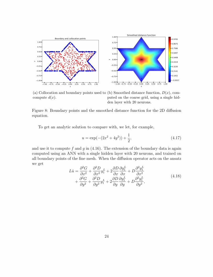
In this case, Γ = ∂Ω and the smoothed distance function is computed using all pointsalong the boundary as seen in Figure 8.

23

1.00 0.75 0.50 0.25 0.00 0.25 0.50 0.75 1.00x

1.00

0.75

0.50

0.25

0.00

0.25

0.50

0.75

1.00

y

Boundary and collocation points

(a) Collocation and boundary points used tocompute d(x).

1.00 0.75 0.50 0.25 0.00 0.25 0.50 0.75 1.00x

1.00

0.75

0.50

0.25

0.00

0.25

0.50

0.75

1.00

y

Smoothed distance function

0.0037

0.1052

0.2141

0.3230

0.4319

0.5408

0.6497

0.7586

0.8675

0.9765

(b) Smoothed distance function, D(x), com-puted on the coarse grid, using a single hid-den layer with 20 neurons.

Figure 8: Boundary points and the smoothed distance function for the 2D diffusionequation.

To get an analytic solution to compare with, we let, for example,

u = exp(−(2x2 + 4y2)) +1

2, (4.17)

and use it to compute f and g in (4.16). The extension of the boundary data is againcomputed using an ANN with a single hidden layer with 20 neurons, and trained onall boundary points of the fine mesh. When the diffusion operator acts on the ansatzwe get

Lu =∂2G

∂x2+∂2D

∂x2yL1 + 2

∂D

∂x

∂yL1∂x

+D∂2yL1∂x2

+∂2G

∂y2+∂2D

∂y2yL1 + 2

∂D

∂y

∂yL1∂y

+D∂2yL1∂y2

,

(4.18)

24

and the gradients of the residual cost function becomes

∂C

∂wljk

= (Lu− f)

(∂2D

∂x2

∂yL1∂wl

jk

+ 2∂D

∂x

∂2yL1∂x∂wl

jk

+D∂3yL1

∂x2∂wljk

)

+ (Lu− f)

(∂2D

∂y2

∂yL1∂wl

jk

+ 2∂D

∂y

∂2yL1∂y∂wl

jk

+D∂3yL1

∂y2∂wljk

),

∂C

∂blj= (Lu− f)

(∂2D

∂x2

∂yL1∂blj

+ 2∂D

∂x

∂2yL1∂x∂blj

+D∂3yL1∂x2∂blj

)

+ (Lu− f)

(∂2D

∂y2

∂yL1∂blj

+ 2∂D

∂y

∂2yL1∂y∂blj

+D∂3yL1∂y2∂blj

).

(4.19)

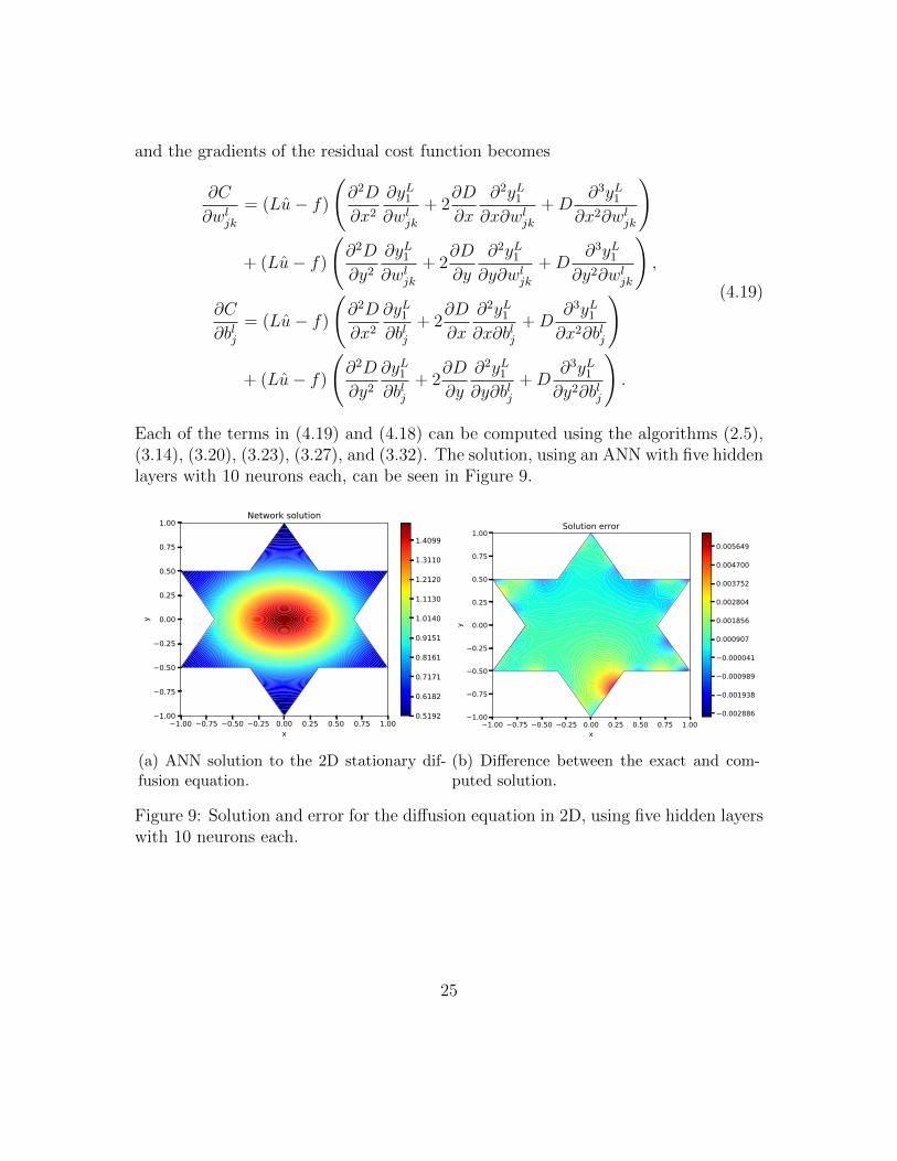
Each of the terms in (4.19) and (4.18) can be computed using the algorithms (2.5),(3.14), (3.20), (3.23), (3.27), and (3.32). The solution, using an ANN with five hiddenlayers with 10 neurons each, can be seen in Figure 9.

1.00 0.75 0.50 0.25 0.00 0.25 0.50 0.75 1.00x

1.00

0.75

0.50

0.25

0.00

0.25

0.50

0.75

1.00

y

Network solution

0.5192

0.6182

0.7171

0.8161

0.9151

1.0140

1.1130

1.2120

1.3110

1.4099

(a) ANN solution to the 2D stationary dif-fusion equation.

1.00 0.75 0.50 0.25 0.00 0.25 0.50 0.75 1.00x

1.00

0.75

0.50

0.25

0.00

0.25

0.50

0.75

1.00

y

Solution error

0.002886

0.001938

0.000989

0.000041

0.000907

0.001856

0.002804

0.003752

0.004700

0.005649

(b) Difference between the exact and com-puted solution.

Figure 9: Solution and error for the diffusion equation in 2D, using five hidden layerswith 10 neurons each.

25

4.6 Higher-dimensional problems

Higher-dimensional problems follow the same pattern as the 2D case. For example,in N dimensions we have the diffusion operator acting on the ansatz as

Lu =N∑i=1

(∂2G

∂x2i

+∂2D

∂x2i

yL1 + 2∂D

∂xi

∂yL1∂xi

+D∂yL1∂x2

i

), (4.20)

and the gradients of the residual cost function becomes

∂C

∂wljk

= (Lu− f)N∑i=1

(∂2D

∂x2i

∂yL1∂wl

jk

+ 2∂D

∂xi

∂2yL1∂xi∂wl

jk

+D∂3yL1

∂x2i∂w

ljk

),

∂C

∂blj= (Lu− f)

N∑i=1

(∂2D

∂x2i

∂yL1∂blj

+ 2∂D

∂xi

∂2yL1∂xi∂blj

+D∂3yL1∂x2

i∂blj

).

(4.21)

As we can see, the computational complexity increases linearly with the number ofspace dimensions as there is one additional term added for each dimension. Thenumber of parameters in the deep ANN increases with the number of neurons in thefirst hidden layer for each dimension. For a sufficiently deep ANN, this increase isnegligible.

The main cause for increased computational time is the number of collocationpoints. Regular grids grows exponentially with the number of dimensions and quicklybecomes infeasible. Uniformly random numbers in high-dimensions are in fact notuniformly distributed across the whole space, but tends to cluster on hyperplanes,thus providing a poor coverage of the whole space. This is a well-known fact forMonto Carlo methods, and led to the development of sequences of quasi-randomnumbers called low discrepancy sequences. See for example ch. 2 in [32], or [4, 35]and references therein.

There are plenty of different low discrepancy sequences, and an evaluation of theirefficiency in the context of deep ANNs is beyond the scope of this paper. A commonchoice is the Sobol sequence [34] which is described in detail in [2] for N ≤ 40, andlater extended in [14] and [15] for N ≤ 1111, and N ≤ 21201, respectively. To com-pute a high-dimensional problem we thus generate Nd points from a Sobol sequencein N dimensions to use as collocation points, and Nb points in N − 1 dimensions touse as boundary points. The rest follows the same procedure as previously described.

A few more examples of work on high-dimensional problems and deep neuralnetworks for PDEs can be found in [33, 10, 6].

26

5 Convergence considerations

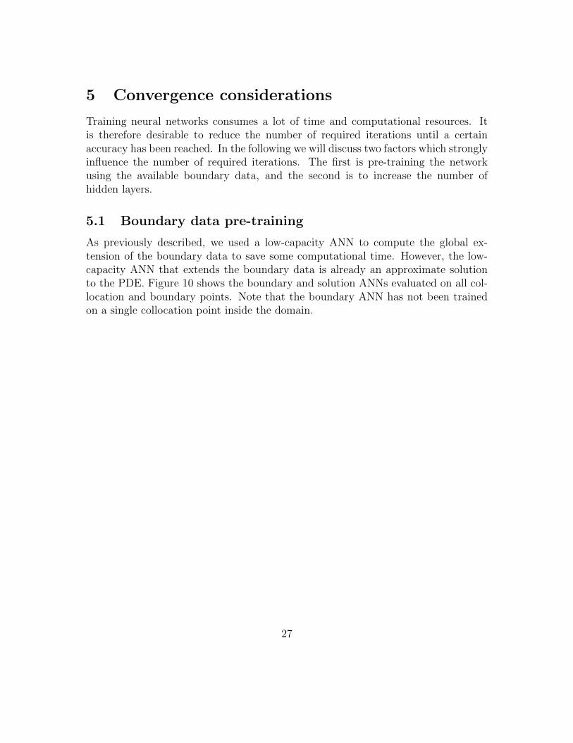
Training neural networks consumes a lot of time and computational resources. Itis therefore desirable to reduce the number of required iterations until a certainaccuracy has been reached. In the following we will discuss two factors which stronglyinfluence the number of required iterations. The first is pre-training the networkusing the available boundary data, and the second is to increase the number ofhidden layers.

5.1 Boundary data pre-training

As previously described, we used a low-capacity ANN to compute the global ex-tension of the boundary data to save some computational time. However, the low-capacity ANN that extends the boundary data is already an approximate solutionto the PDE. Figure 10 shows the boundary and solution ANNs evaluated on all col-location and boundary points. Note that the boundary ANN has not been trainedon a single collocation point inside the domain.

27

1.00 0.75 0.50 0.25 0.00 0.25 0.50 0.75 1.00x

1.00

0.75

0.50

0.25

0.00

0.25

0.50

0.75

1.00y

Boundary data extension

0.4186

0.3145

0.2105

0.1064

0.0023

0.1018

0.2058

0.3099

0.4140

0.5181

(a) Boundary data extension for the advec-tion equation.

1.00 0.75 0.50 0.25 0.00 0.25 0.50 0.75 1.00x

1.00

0.75

0.50

0.25

0.00

0.25

0.50

0.75

1.00

y

Network solution

0.5005

0.3994

0.2983

0.1973

0.0962

0.0049

0.1060

0.2070

0.3081

0.4092

(b) Network solution of the advection equa-tion.

1.00 0.75 0.50 0.25 0.00 0.25 0.50 0.75 1.00x

1.00

0.75

0.50

0.25

0.00

0.25

0.50

0.75

1.00

y

Boundary data extension

0.5189

0.6059

0.6930

0.7801

0.8672

0.9543

1.0414

1.1284

1.2155

1.3026

(c) Boundary data extension for the diffusionequation.

1.00 0.75 0.50 0.25 0.00 0.25 0.50 0.75 1.00x

1.00

0.75

0.50

0.25

0.00

0.25

0.50

0.75

1.00

y

Network solution

0.5192

0.6182

0.7171

0.8161

0.9151

1.0140

1.1130

1.2120

1.3110

1.4099

(d) Network solution of the diffusion equa-tion.

Figure 10: The boundary ANNs use a single hidden layer with 20 neurons, trainedonly on the boundary points. The solution ANNs use five hidden layers with 10neurons each, trained on both the boundary and collocation points.

As fitting an ANN to the boundary data is an order of magnitude faster thansolving the PDE, this suggests that we can pre-train the solution ANN by fitting itto the boundary data. It is still a good idea to keep the boundary ANN as a separatelow-capacity ANN as it will speed up the training of the solution ANN due to themany evaluations that is required during training.

When training with the BFGS method, pre-training has limited effect due to theefficiency of the method to quickly reduce the value of the cost function. For less

28

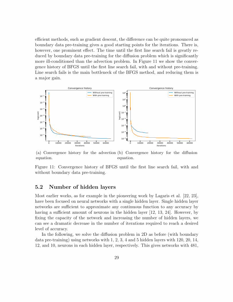
efficient methods, such as gradient descent, the difference can be quite pronounced asboundary data pre-training gives a good starting points for the iterations. There is,however, one prominent effect. The time until the first line search fail is greatly re-duced by boundary data pre-training for the diffusion problem which is significantlymore ill-conditioned than the advection problem. In Figure 11 we show the conver-gence history of BFGS until the first line search fail, with and without pre-training.Line search fails is the main bottleneck of the BFGS method, and reducing them isa major gain.

0 10000 20000 30000 40000 50000 60000Iterations

10 7

10 6

10 5

10 4

10 3

10 2

10 1

log(

cost

)

Convergence historyWithout pre-trainingWith pre-training

(a) Convergence history for the advectionequation.

0 10000 20000 30000 40000 50000 60000Iterations

10 5

10 4

10 3

10 2

10 1

100

101

102

log(

cost

)

Convergence historyWithout pre-trainingWith pre-training

(b) Convergence history for the diffusionequation.

Figure 11: Convergence history of BFGS until the first line search fail, with andwithout boundary data pre-training.

5.2 Number of hidden layers

Most earlier works, as for example in the pioneering work by Lagaris et al. [22, 23],have been focused on neural networks with a single hidden layer. Single hidden layernetworks are sufficient to approximate any continuous function to any accuracy byhaving a sufficient amount of neurons in the hidden layer [12, 13, 24]. However, byfixing the capacity of the network and increasing the number of hidden layers, wecan see a dramatic decrease in the number of iterations required to reach a desiredlevel of accuracy.

In the following, we solve the diffusion problem in 2D as before (with boundarydata pre-training) using networks with 1, 2, 3, 4 and 5 hidden layers with 120, 20, 14,12, and 10, neurons in each hidden layer, respectively. This gives networks with 481,

29

501, 477, 517, and 481 trainable parameters (weights and biases), respectively, whichwe consider comparable. The networks are trained until the cost is less than 10−5,and we record the number of required iterations. The result can be seen in Figure 12.We can clearly see how the number of required iterations decreases as we increasethe number of hidden layers. At five hidden layers, we are starting to experience thevanishing gradient problem [8], and the convergence starts to deteriorate. Note thatusing a single hidden layer we did not reach the required tolerance until we exceededthe maximum number of allowed iterations.

0 50000 100000 150000 200000Iterations

10 5

10 4

10 3

10 2

10 1

100

101

102

log(

cost

)

Convergence history1 hidden layer2 hidden layers3 hidden layers4 hidden layers5 hidden layers

Figure 12: Number of iterations required for increasing network depth.

6 Summary, conclusion and future research

We have presented a method for solving advection and diffusion type partial dif-ferential equations in complex geometries using deep feedforward artificial neuralnetworks. We have derived analytical expressions for the gradients of the cost func-tion with respect to the network parameters, and the gradients of the network itselfwith respect to the input, for arbitrarily deep networks. By following our derivations,one can extend this work to include non-linear systems of PDEs of arbitrary orderwith mixed derivatives.

30

We conducted numerical experiments with different network depths and it is clearthat increasing the number of hidden layers is beneficial for the number of trainingiterations required to reach a certain accuracy. The effects will be even more pro-nounced when adding deep learning techniques that prevents the vanishing gradientproblem. Extending the feedforward network to more complex configurations, us-ing for example convolutional layers, dropout, and batch normalization is the topicof future work to develop even deeper networks and study the layer-wise variationswhen changing different parts of the PDE.

As a more speculative note on future research we recall that is a well-know fact,in for example image analysis, that the different layers of deep ANN are responsiblefor detecting different features [9, 27, 28]. One can pose the question if somethingsimilar occurs in the context of PDEs. In general a boundary value problem for aPDE consists of the following features: a differential operator (the PDE), geometry,a boundary operator and boundary data. An interesting problem could be to studythe effect on the different layers when varying the features of the PDE.

For example, consider the 2D diffusion problem,

k

(∂2u

∂x2+∂2u

∂y2

)= f, x ∈ Ω(s),

u = τg, x ∈ ∂Ω(s),

(6.1)

where we have parameterized the differential operator by a diffusion coefficient k, thedomain and the boundary data by s, τ ∈ [0, 1], respectively. The shape parameters transforms the domain from one shape to another. We can then compute thevariance of the weights and biases as we are varying k, s, τ by,

Var(W l) =∑i

||W li −W l

i−1||F||W l

0||F,

Var(bl) =∑i

||bli − bli−1||||bl0||

,

(6.2)

where, for example, || · ||F is the Frobenius norm, and || · || the usual Euclidean vectornorm, and W l

i , bli denotes the weights and biases of layer l for k = ki, s = si, or

τ = τi.Experiments show that the variances defined are very sensitive to the local mini-

mum found by the optimizer and we have not been able to clearly see the layer-wisevariance. Moreover, in the case of feedforward ANN the vanishing gradient problemcauses the layers to train at different speeds which makes it difficult to separate a

31

poor local minimum from the actual effect of varying the different features. However,it could still possible to train a base network and to re-train only some layers de-pending on which feature of the PDE that is changing. Our results suggest that oneshould strive to train even deeper networks by deploying a variety of methods andtechniques that have been developed over the past decade to overcome the difficultiesin training deep networks.

References

[1] J. L. Bentley. Multidimensional binary search trees used for associative search-ing. Commun. ACM, 18(9):509–517, Sept. 1975.

[2] P. Bratley and B. L. Fox. Algorithm 659: Implementing Sobol’s quasirandomsequence generator. ACM Trans. Math. Softw., 14(1):88–100, Mar. 1988.

[3] P. Chaudhari, A. Oberman, S. Osher, S. Soatto, and G. Carlier. Deep relaxation:partial differential equations for optimizing deep neural networks. ArXiv e-prints, Apr. 2017.

[4] J. Cheng and M. J. Druzdzel. Computational investigation of low-discrepancysequences in simulation algorithms for Bayesian networks. ArXiv e-prints, Jan.2013.

[5] N. E. Cotter. The Stone–Weierstrass theorem and its application to neuralnetworks. IEEE Transactions on Neural Networks, 1(4):290–295, Dec. 1990.

[6] W. E, J. Han, and A. Jentzen. Deep learning-based numerical methods forhigh–dimensional parabolic partial differential equations and backward stochas-tic differential equations. ArXiv e-prints, June 2017.

[7] R. Fletcher. Practical methods of optimization. Wiley, 2nd edition, 1987.

[8] X. Glorot and Y. Bengio. Understanding the difficulty of training deep feedfor-ward neural networks. In Proceedings of the Thirteenth International Conferenceon Artificial Intelligence and Statistics, pages 249–256. PMLR, 2010.

[9] I. J. Goodfellow, Q. V. Le, A. M. Saxe, H. Lee, and A. Y. Ng. Measuring invari-ances in deep networks. In Proceedings of the 22nd International Conference onNeural Information Processing Systems, pages 646–654. Curran Associates Inc.,2009.

32

[10] J. Han, A. Jentzen, and W. E. Overcoming the curse of dimensionality: Solvinghigh-dimensional partial differential equations using deep learning. ArXiv e-prints, July 2017.

[11] G. E. Hinton, S. Osindero, and Y.-W. Teh. A fast learning algorithm for deepbelief nets. Neural Computation, 18(7):1527–1554, 2006.

[12] K. Hornik, M. Stinchcombe, and H. White. Multilayer feedforward networksare universal approximators. Neural Networks, 2(5):359–366, 1989.

[13] K. Hornik, M. Stinchcombe, and H. White. Universal approximation of anunknown mapping and its derivatives using multilayer feedforward networks.Neural Networks, 3(5):551–560, 1990.

[14] S. Joe and F. Y. Kuo. Remark on algorithm 659: Implementing Sobol’s quasir-andom sequence generator. ACM Trans. Math. Softw., 29(1):49–57, Mar. 2003.

[15] S. Joe and F. Y. Kuo. Constructing Sobol sequences with better two-dimensionalprojections. SIAM Journal on Scientific Computing, 30(5):2635–2654, 2008.

[16] C. Johnson and J. Saranen. Streamline diffusion methods for the incompressibleEuler and Navier–Stokes equations. Mathematics of Computation, 47(175):1–18,1986.

[17] E. Jones, T. Oliphant, P. Peterson, et al. SciPy: Open source scientific tools forPython. http://www.scipy.org, 2001–. Accessed 2017-07-07.

[18] G. Klambauer, T. Unterthiner, A. Mayr, and S. Hochreiter. Self-normalizingneural networks. ArXiv e-prints, June 2017.

[19] H.-O. Kreiss. Initial boundary value problems for hyperbolic systems. Commu-nications on Pure and Applied Mathematics, 23(3):277–298, 1970.

[20] A. Krizhevsky, I. Sutskever, and G. E. Hinton. Imagenet classification with deepconvolutional neural networks. In Advances in Neural Information ProcessingSystems 25, pages 1097–1105. Curran Associates, Inc., 2012.

[21] M. Kumar and N. Yadav. Multilayer perceptrons and radial basis function neuralnetwork methods for the solution of differential equations: A survey. Computers& Mathematics with Applications, 62(10):3796–3811, 2011.

33

[22] I. E. Lagaris, A. Likas, and D. I. Fotiadis. Artificial neural networks for solv-ing ordinary and partial differential equations. IEEE Transactions on NeuralNetworks, 9(5):987–1000, Sept. 1998.

[23] I. E. Lagaris, A. C. Likas, and D. G. Papageorgiou. Neural-network methodsfor boundary value problems with irregular boundaries. IEEE Transactions onNeural Networks, 11(5):1041–1049, Sept. 2000.

[24] X. Li. Simultaneous approximations of multivariate functions and their deriva-tives by neural networks with one hidden layer. Neurocomputing, 12(4):327–343,1996.

[25] W. S. McCulloch and W. Pitts. A logical calculus of the ideas immanent innervous activity. The bulletin of mathematical biophysics, 5(4):115–133, Dec.1943.

[26] K. S. McFall and J. R. Mahan. Artificial neural network method for solution ofboundary value problems with exact satisfaction of arbitrary boundary condi-tions. IEEE Transactions on Neural Networks, 20(8):1221–1233, Aug. 2009.

[27] G. Montavon, M. L. Braun, and K.-R. Muller. Kernel analysis of deep networks.J. Mach. Learn. Res., 12:2563–2581, Nov. 2011.

[28] K. R. Muller, S. Mika, G. Ratsch, K. Tsuda, and B. Scholkopf. An introductionto kernel-based learning algorithms. IEEE Transactions on Neural Networks,12(2):181–201, Mar. 2001.

[29] S. M. Omohundro. Five balltree construction algorithms. Technical report,International Computer Science Institute, 1989.

[30] K. Rudd and S. Ferrari. A constrained integration (cint) approach to solvingpartial differential equations using artificial neural networks. Neurocomputing,155:277–285, 2015.

[31] K. Rudd, G. Muro, and S. Ferrari. A constrained backpropagation approach forthe adaptive solution of partial differential equations. IEEE Transactions onNeural Networks and Learning Systems, 25(3):571–584, 2014.

[32] R. Seydel. Tools for Computational Finance. Universitext (1979). Springer,2004.

34

[33] J. Sirignano and K. Spiliopoulos. DGM: A deep learning algorithm for solvingpartial differential equations. ArXiv e-prints, Aug. 2017.

[34] I. M. Sobol. On the distribution of points in a cube and the approximateevaluation of integrals. USSR Computational Mathematics and MathematicalPhysics, 7(4):86–112, 1967.

[35] X. Wang and I. H. Sloan. Low discrepancy sequences in high dimensions: Howwell are their projections distributed? J. Comput. Appl. Math., 213:366–386,Mar. 2008.

[36] N. Yadav, A. Yadav, and M. Kumar. An Introduction to Neural Network Meth-ods for Differential Equations. Springer Briefs in Applied Sciences and Technol-ogy. Springer Netherlands, 2015.

35