a unified approach to theory reasoningusers.cecs.anu.edu.au/~baumgart/publications/thover.pdf ·...
TRANSCRIPT

A Unified Approach to Theory Reasoning
Peter Baumgartner, Ulrich FurbachUniversitat Koblenz
Rheinau 3–4W-5400 Koblenz
{peter,uli}@infko.uni-koblenz.de
Uwe PetermannUniversitaet LeipzigAugustusplatz 10/11
O-7010 [email protected]
Abstract. Theory reasoning is a kind of two-level reasoning in automated theoremproving, where the knowledge of a given domain or theory is separated and treated byspecial purpose inference rules. We define a classification for the various approaches fortheory reasoning which is based on the syntactic concepts of literal level — term level— variable level. The main part is a review of theory extensions of common calculi(resolution, model elimination and a connection method). In order to see the relationshipsamong these calculi, we define a super-calculus called theory consolution. Completenessof the various theory calculi is proven. Finally, due to its relevance in automated reasoning,we describe current ways of equality handling.
Contents
1 Introduction 2
2 The Tour: Literal level – Term level – Variable level 52.1 Literal Level Theory Reasoning � � � � � � � � � � � � � � � � � � � � � � � � � � � � 52.2 Term Level Theory Reasoning � � � � � � � � � � � � � � � � � � � � � � � � � � � � � 82.3 Variable Level Theory Reasoning – Constraints � � � � � � � � � � � � � � � � � � � � 10
3 Literal Level Theory Reasoning 103.1 Consolution � � � � � � � � � � � � � � � � � � � � � � � � � � � � � � � � � � � � � � 113.2 Theory Consolution � � � � � � � � � � � � � � � � � � � � � � � � � � � � � � � � � � 173.3 Partial Theory Consolution � � � � � � � � � � � � � � � � � � � � � � � � � � � � � � � 223.4 Theory Resolution � � � � � � � � � � � � � � � � � � � � � � � � � � � � � � � � � � � 243.5 Theory Model Elimination � � � � � � � � � � � � � � � � � � � � � � � � � � � � � � � 363.6 Theory connection method � � � � � � � � � � � � � � � � � � � � � � � � � � � � � � � 43
1 Introduction 2
4 Equality 514.1 Dealing with Equality via Total Theory Reasoning � � � � � � � � � � � � � � � � � � 514.2 Dealing with Equality via Partial Theory Reasoning � � � � � � � � � � � � � � � � � � 54
5 Conclusion 62
1 Introduction
One of the most traditional disciplines in AI is Theorem Proving. In the early days it wasconcentrated mainly on developing general proof procedures for predicate logic. According tothe shift within wide parts of AI-research towards special domain dependent systems, automatedreasoning and theorem proving nowadays aim at incorporating specialized and efficient moduls,which are suited for handling special parts or domains of knowledge. Whenever this is donein a formal way we will understand those moduls as a means to built-in theories and speak of“theory reasoning”.
A very prominent example for efficient handling of a theory is equality handling. There is asimple way of specifying this theory, namely by stating the axioms of reflexivity, symmetry,transitivity and by stating the substitutivity of function and predicate symbols. If these formulasare added to the formulas to be proven by the system, the usual inference rules are able toprocess this theory. A better approach is to supply special inference rules for handling theequality predicate with respect to the equality theory, like e.g. paramodulation (Robinson andWos, 1969) or RUE-resolution (Digricoli and Harrison, 1986).
Another very well-investigated example for theory handling is the design of calculi and proofprocedures, which use many- or order-sorted logics (Blasius and Burckert, 1989). Here, theaim is to take care of a sort hierarchy in a direct way, e.g. by using a special unificationprocedure. This is in contrast to relativation approaches which transform the sort informationinto formulas of the unsorted logics.
While the above two examples were concerned mainly with an efficient treatment of a theory,there is as well a concern in the field of knowledge engineering of keeping different kindsof knowledge apart. Often, one wants to separate taxonomical from assertional knowledge:taxonomical knowledge is used as a special theory, which has to be handled outside thededuction mechanism which processes the assertional knowledge. One of the most prominentexamples of those approaches is KRYPTON (Brachmann et al., 1983), where the semantic netlanguage KL-ONE is used as a theory defining language, which is combined with a theoremprover for predicate logic. This system is based on the theory resolution calculus (Stickel,1985), which will be discussed later on. Nowadays numerous works on defining conceptlanguages with well-understood semantics for the definition of taxonomical knowledge exist(Hollunder, 1990).
1 Introduction 3
Viewpoint of this paper
The aim of this paper is twofold: Firstly, we want to classify the various kinds of treatingtheories within deduction systems, and secondly, we want to compare a special subclass ofthese methods. It is easier to compare the theory reasoning calculi if a common input languagecan be presupposed. Fortunately, the calculi to be discussed operate on formulas in a standardlanguage, which is, of course, clause logic. Thus clause logic will serve us well as a commoninput language, too. However there are minor differences: sometimes clauses are thoughtof as sets of literals, sometimes of multisets and sometimes of sequences. Fortunately thesedifferences are not essential for the intuitive understanding of theory reasoning, and so thediscussion of these differences can be postponed to the formal section. As a coincidence mostwork is done in a refutational setting, but not in an affirmative one. Due to their perfectduality, it suffices to restrict attention to one of these concepts. This will be the more commonrefutational setting.
Theory reasoning always deals with two kinds of reasoning: background reasoning for thetheory, and foreground reasoning for the actual problem specification. We are mostly interestedin studying the interface between foreground and background reasoning. We give a formaldescription of this interface which applies to a wide class of theories. We will not focus on thequestion of how to built dedicated background reasoners for special theories (equality will bean exception).
It has to be said what kinds of theories we are interested in. The “upper bound” is given bythe universal theories, i.e. theories that can be axiomatized by a set of formulas that does notcontain
�-quantifiers. Universal theories are expressive enough to formulate e.g. equality or
interesting taxonomic theories. Moreover, the restriction to universal theories is not essential.A theory which contains existential quantifiers may be transformed by Skolemization into auniversal theory which is equivalent up to an extension of the signature by Skolem functions.Universal theories also mark the limit of what can be built into a calculus preserving thecompleteness of calculus (cf. (Petermann, 1991b)).
We do not treat reasoning in single models, like real numbers and their arithmetic, or classesof models. Such extensions of theory reasoning have been investigated in (Burckert, 1990a).
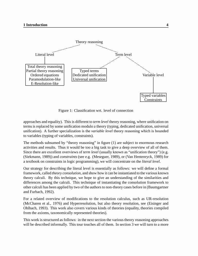
Due to the great variety of approaches for theory reasoning, we prefer to bring in structure byclassifying the various approaches. Of course there are plenty ways of doing. The classificationwe use is by level of connection. In order to explain this term it is necessary to recall the natureof theory reasoning as interfacing background reasoning and foreground reasoning. Now, by“level of connection” we mean the common subpart of the foreground and the backgroundlanguage, that is used for their interfacing. To be concrete, we will distinguish the three levelsliteral level, term level and variable level. Figure (1) is a classification of the approaches to bedescribed with respect to level of connection. The literal level is the most general of all; it allowsfor theory reasoning with literals with different predicate symbols (general theory reasoning
1 Introduction 4
Theory reasoning
Literal level Term level
Total theory reasoningPartial theory reasoning
Ordered equationsParamodulation-like
E-Resolution-like
Typed termsDedicated unificationUniversal unification
Variable level
Typed variablesConstraints
� � � � � � � � � � � � � � � � � � � � � �� � � � � � � � � �
��
��
��
��
��
��
� ��
��
��
��
��
��
��
�
� �
� �
� �
� �
� �
� �
Figure 1: Classification wrt. level of connection
approaches and equality). This is different to term level theory reasoning, where unification onterms is replaced by some unification modulo a theory (typing, dedicated unification, universalunification). A further specialization is the variable level theory reasoning which is boundedto variables (typing of variables, constraints).
The methods subsumed by “theory reasoning” in figure (1) are subject to enormous researchactivities and results. Thus it would be too a big task to give a deep overview of all of them.Since there are excellent overviews of term level (usually known as “unification theory”) (e.g.(Siekmann, 1989)) and constraints (see e.g. (Meseguer, 1989), or (Van Hentenryck, 1989) fora textbook on constraints in logic programming), we will concentrate on the literal level.
Our strategy for describing the literal level is essentially as follows: we will define a formalframework, called theory consolution, and show how it can be instantiated to the various knowntheory calculi. By this technique, we hope to give an understanding of the similarities anddifferences among the calculi. This technique of instantiating the consolution framework toother calculi has been applied by two of the authors to non-theory cases before in (Baumgartnerand Furbach, 1992).
For a related overview of modifications to the resolution calculus, such as UR-resolution(McCharen et al., 1976) and Hyperresolution, but also theory resolution, see (Eisinger andOhlbach, 1993). This work also covers various kinds of theories (equality, theories compiledfrom the axioms, taxonomically represented theories).
This work is structured as follows: in the next section the various theory reasoning approacheswill be described informally. This tour touches all of them. In section 3 we will turn to a more
2 The Tour: Literal level – Term level – Variable level 5
formal presentation of the literal level. As just mentioned, this will be done on the basis of onespecial calculus, namely the consolution calculus. It will be presented first in its non-theoryversion and finally we define its total and its partial variant. This calculi will be used afterwardsto discuss theory resolution, theory model elimination and a theory connection method. Thecompleteness of these calculi is proven rigorously by mapping our presentation of the calculito corresponding representations, for which we have completeness results. Section 4 containsa discussion on equality handling.
2 The Tour: Literal level – Term level – Variable level
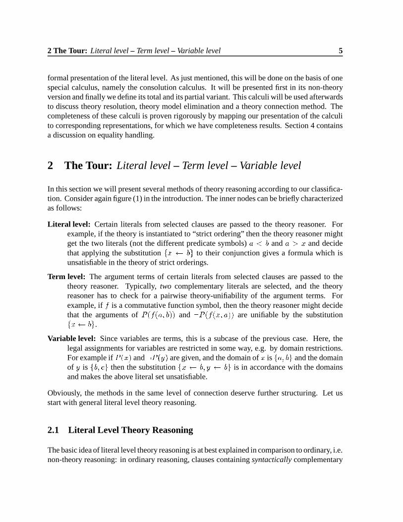
In this section we will present several methods of theory reasoning according to our classifica-tion. Consider again figure (1) in the introduction. The inner nodes can be briefly characterizedas follows:
Literal level: Certain literals from selected clauses are passed to the theory reasoner. Forexample, if the theory is instantiated to “strict ordering” then the theory reasoner mightget the two literals (not the different predicate symbols) � � � and � � � and decidethat applying the substitution � � � � � to their conjunction gives a formula which isunsatisfiable in the theory of strict orderings.
Term level: The argument terms of certain literals from selected clauses are passed to thetheory reasoner. Typically, two complementary literals are selected, and the theoryreasoner has to check for a pairwise theory-unifiability of the argument terms. Forexample, if � is a commutative function symbol, then the theory reasoner might decidethat the arguments of � � � � � � and � � � � � � are unifiable by the substitution� � � � � .
Variable level: Since variables are terms, this is a subcase of the previous case. Here, thelegal assignments for variables are restricted in some way, e.g. by domain restrictions.For example if � � and � � are given, and the domain of � is � � � � � and the domainof � is � � � � � then the substitution � � � � � � � � � is in accordance with the domainsand makes the above literal set unsatisfiable.
Obviously, the methods in the same level of connection deserve further structuring. Let usstart with general literal level theory reasoning.
2.1 Literal Level Theory Reasoning
The basic idea of literal level theory reasoning is at best explained in comparison to ordinary, i.e.non-theory reasoning: in ordinary reasoning, clauses containing syntactically complementary

2.1 Literal Level Theory Reasoning 6
Literal leveltheory reasoning
General Theories
Partialtheory reasoning
��
��� �
��
��
Totaltheory reasoning
� � � � � � �� � � � � � � ��Equality
Orderedequations
����� �
����
Non-orderedequations
Paramodulation-like
��
��� �
��
��
E-Resolution-like
Figure 2: Classification of “Literal level”
literals are used for inferences, whereas in theory reasoning this is done with semanticallycomplementary literals. Here “semantically complementary” means roughly “unsatisfiable inthe given theory”. A precise characterization is given in the next section.
Figure (2) depicts a classification of literal level theory reasoning. On the one hand we willconsider general theory reasoning approaches. There, no fixed theory is presupposed, andthese frameworks can be instantiated with a great variety of theories. On the other hand wewill devote an extra section to equality, i.e. general theory reasoning that is instantiated withthe theory of equality. This partition is motivated by the enormous research dedicated toequality.
General literal level theory reasoning (simply called “theory reasoning” from now on in thissubsection) is the most general technique of all. It is a scheme of building in arbitrary universaltheories into first order calculi. Still on this very general level two variants can be distinguished(figure 2):
Partial theory reasoning: Viewed operationally, in a partial reasoning step the backgroundreasoner is passed from the foreground reasoner a set of literals and returns a formula.This formula is a new subgoal to be proved. It is also called residue. For example, if thetheory is “strict ordering” and we are given the literals � � � � � � � � � � � � � � � andthe “goal” � � � . By transitivity of � the literal � � � is a logical consequence of � ,and this literal immediately contradicts the goal. To show this fact with partial theoryreasoning the background reasoner might be passed the goal � � � and the literal � � �from � ; then it returns the residue � � � . For the next step this residue plays the same
2.1 Literal Level Theory Reasoning 7
role as the goal before. This kind of reasoning is repeated until a contradiction becomesimmediate.
Semantically, a residue states a logical consequence of the passed literals, or, in otherwords, the negation of the residue together with the passed literals is unsatisfiable in thetheory. As usual, in the non-ground case substitutions are involved. See section (3) fora precise treatment of residues and so-called “theory refuting substitutions”.
Total theory reasoning: Total theory reasoning is the same as partial theory reasoning, exceptthat the residue must be empty. Thus, the literal set passed to the background reasonermust be unsatisfiable by itself. For example, the literals � � � and � � � are unsatisfiablein the theory of strict orderings, and thus are subject to a total theory reasoning step.
The distinction between these kinds of theory reasoning is important for several reasons:firstly, in partial theory reasoning we have the unique situation that the theory reasoner returnsa formula to the caller, and not just a substitution or a yes-no result. Thus the coupling is moresymmetric than the other approaches on the term level.Secondly, for undecidable theories total theory reasoning requires too much from the theoryreasoner, i.e. the inference must neccessarily be undecidable. As a consequence, the notion of“derivation” is undecidable — a highly undesirable property. This implies for implementationsthat the background reasoner cannot be “called” as a procedure that is guaranteed to terminate.But even if the theory is decidable there remain problems with total theory reasoning. Forexample let us consider the theory of equality. Though this theory admits a decision procedurefor the background reasoner, as e.g. rigid � -unification (cf. (Gallier and Snyder, 1990) andsection 4 of the present paper), it cannot be predicted by the foreground reasoner how manyvariants of literals from clauses constitute a contradictory set. In other words: it is hard tofind good candidates for contradictory sets. On the other hand, it may not be difficult forthe foreground reasoner to detect the potential kernel of a contradictory set. Moreover, thetheory reasoner might guide the search for literals which complete the kernel to a contradictoryset. This scheme of co-operation with a search guiding role of the theory reasoner is the ideaof partial theory reasoning. The residue returned by the partial reasoner gives advice to thegeneral reasoner for the search for appropriate literals.
The generality of theory reasoning is both a strength and a weakness: it is a strength, because itsubsumes all other techniques if an appropriate theory reasoner is given — and the generalityis a weakness because it cannot propose how to come to efficient theory reasoners, which areusually domain dependent.
Since Stickel’s pioneering work for the resolution calculus (Stickel, 1985; Stickel, 1983),the scheme was ported to many calculi. It was done for matrix methods in (Murray andRosenthal, 1987), for the connection method in (Petermann, 1990) and for model eliminationin (Baumgartner, 1992a). The latter two papers contain completeness results for the first-ordercase. The primary concern of these works is the combination of the main calculus with thetheory reasoner; it is not the construction of efficient theory reasoners.
2.2 Term Level Theory Reasoning 8
Term leveltheory reasoning
Non-equational theories
Typed terms
��
��
�� ��
� ���
Equational theories
Dedicatedunification
����� �
����
Universalunification
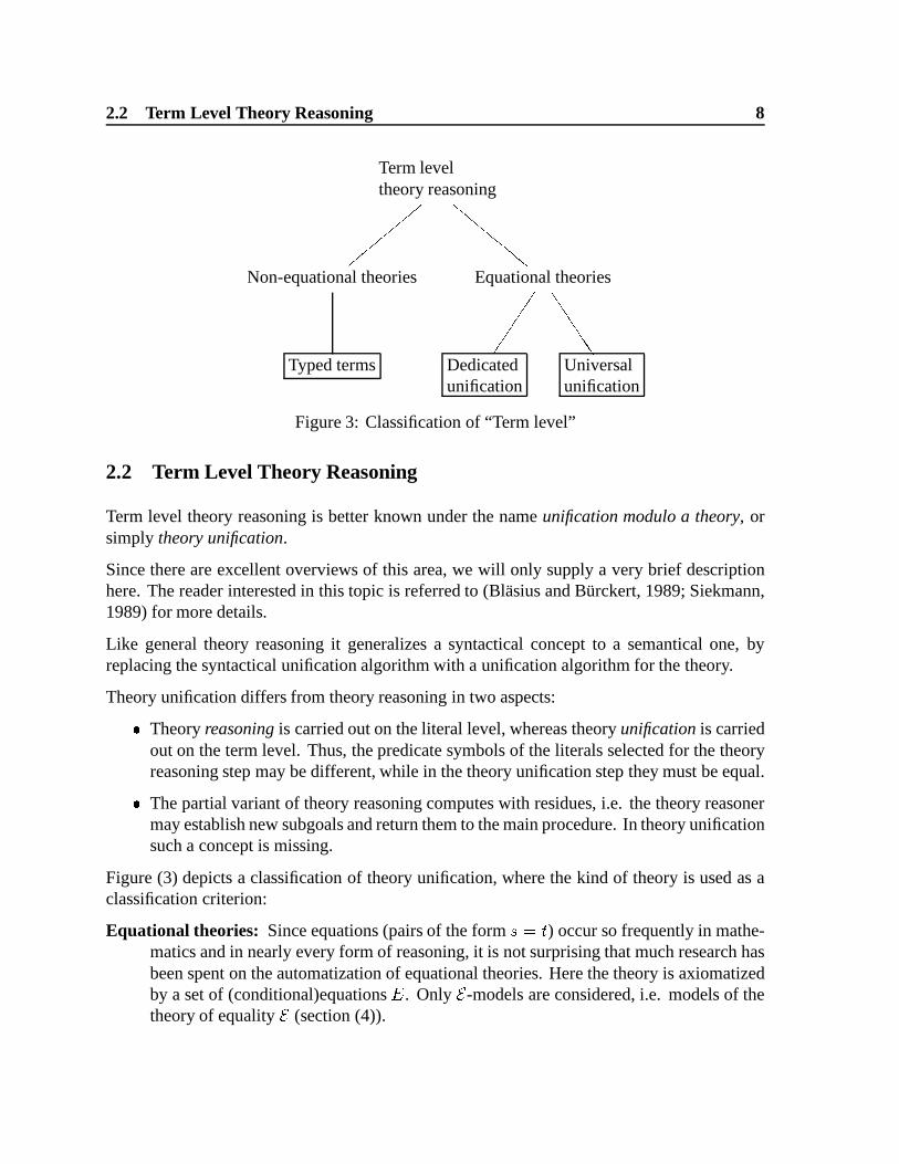
Figure 3: Classification of “Term level”
2.2 Term Level Theory Reasoning
Term level theory reasoning is better known under the name unification modulo a theory, orsimply theory unification.
Since there are excellent overviews of this area, we will only supply a very brief descriptionhere. The reader interested in this topic is referred to (Blasius and Burckert, 1989; Siekmann,1989) for more details.
Like general theory reasoning it generalizes a syntactical concept to a semantical one, byreplacing the syntactical unification algorithm with a unification algorithm for the theory.
Theory unification differs from theory reasoning in two aspects:� Theory reasoning is carried out on the literal level, whereas theory unification is carried
out on the term level. Thus, the predicate symbols of the literals selected for the theoryreasoning step may be different, while in the theory unification step they must be equal.
� The partial variant of theory reasoning computes with residues, i.e. the theory reasonermay establish new subgoals and return them to the main procedure. In theory unificationsuch a concept is missing.
Figure (3) depicts a classification of theory unification, where the kind of theory is used as aclassification criterion:
Equational theories: Since equations (pairs of the form � � � ) occur so frequently in mathe-matics and in nearly every form of reasoning, it is not surprising that much research hasbeen spent on the automatization of equational theories. Here the theory is axiomatizedby a set of (conditional)equations � . Only � -models are considered, i.e. models of thetheory of equality � (section (4)).

2.2 Term Level Theory Reasoning 9
Thus in equational unification the following � -unification problem has to be solved:
Given a set � of equations and some pairs � � � � � � � . Is there a substitution �such that every � -model satisfying � also satisfies � � � � � � � , or shortly, thatall equations � � � � � � � are � -consequences of � .
Such a � is called � -unifier for � � � � � � � in the theory � . The � -unification problem canequivalently be formulated in a more operational fashion. It is roughly as follows: inorder to solve the above problem, try to transform � � into � � by replacement of subtermswith equal terms as given by � . The � -unifier is obtained by collecting the substitutionsalong the way.
Some questions coming up immediately are the following: is the � -unification problemdecidable? (No); how many such � -unifiers exist? (Countable many); if more thanone exists, can we compute a solution base, i.e. a reasonable small set that implicitlyincludes all other solutions?
A problem similar to � -unification is rigid � -unification. This is a resource-boundedform of � -unification which, loosely, forbids drawing more than one instance of anequation in � when solving an � -unification problem. Rigid � -unification is relevant forbuilding in the theory of equality into general theory reasoning calculi and is discussedin section (4).
Unification procedures for equational theories can be further distinguished: on theone hand, there are dedicated unification algorithms, which are special purpose theoryunification algorithms for one single equational theory (see e.g. (Petermann, 1991a)).For example, there are such algorithms for associative and for commutative theories (see(Burckert et al., 1988) as an anchor). From a practical point of view it would be verypleasing to combine given unification algorithms for different theories in order to obtaina unification algorithm for the theories’ union. Unfortunately this is a highly non-trivialtask. An advanced result allows for the combination of theories with disjunct functionsymbols, but common constant symbols (Ringeissen, 1992).
On the other hand we have universal unification algorithms, that work for a wideclass of equational theories (see (Gallier and Snyder, 1990; Gallier and Snyder, 1989; J.-P. Jouannaud, 1991)). Further advantage can be taken if the equations can be directed intorewrite rules. Then the Narrowing-technique can be used, which is the first order versionof rewriting (Hullot, 1980; W. Nutt and Smolka, 1987; Holldobler, 1989). Generaloverviews of theory unification can be found in (J.-P. Jouannaud, 1991; Siekmann,1989), and a recent text book is (Snyder, 1991).
Non-equational theories – typing: The most investigated non-equational theories (at least,conceptually) are those which employ a type hierarchy on terms, as already discussedin the introduction. This is also known as order-sorted unification. Roughly, if � 1 : � 1

2.3 Variable Level Theory Reasoning – Constraints 10
means that the term � 1 is of type � 1, then the unification of the expressions � 1 : � 1 and� 2 : � 2 succeeds if � 1 and � 2 (Robinson-)unify, and if � 1 and � 2 can both be restrictedto a common subtype. See (J.-P. Jouannaud, 1991) for an overview. Order-sortedlogics has been developed since the 60s (Oberschelp, 1962), and nowadays numerousproof-procedures exist, which demonstrate that order-sortedness increases efficiencysignificantly.
2.3 Variable Level Theory Reasoning – Constraints
In variable level theory reasoning, the set of legal values for variables is limited. This isusually achieved by constraints. Syntactically, constraints are formulas that are attached tosome variables in clauses, and semantically they filter out valid assignments for the variables.During inferences the constraints of the unified variables are combined, and eventually, but notnecessarily immediately, the combined constraints must be solved. In other words, constraintsmay be treated lazily. This is the approach taken in (Burckert, 1990a). Constraints are mostlyinvestigated in the context of logic programming and Prolog (Van Hentenryck, 1989; Jaffar andLassez, 1987), which is so successful that constraint logic programming has been establishedas a field of its own.
3 Literal Level Theory Reasoning
As mentioned previously, this work is strongly biased towards the literal level theory reasoning.This section describes several general calculi for literal level theory reasoning in a formalway. In order to see the similarities and differences among them, we have decided to definethe calculi as instances of some particular common framework. Thus, many notions, suchas “derivation”, “theory refuting substitution” and “residue” only have to be defined once.The common framework is called “theory consolution” and it generalizes the non-theoryconsolution calculus as defined in (Eder, 1991). This calculus was designed as a generalizationof both connection calculi and resolution calculi. In (Baumgartner and Furbach, 1992) it hasbeen proved to be useful as framework to define and to compare various other calculi. Thus itis not surprising that its theory-generalization is well-suited for our purpose.
This section is structured as follow. We introduce the consolution calculus along the lines of(Eder, 1991; Baumgartner and Furbach, 1992) and then define a theory version, both in a totaland a partial variant. These calculi are then modified to obtain theory resolution, theory modelelimination and a theory connection method in order. The partial variant thereof is derivedonly for the case of the resolution calculus. Since the instantiations of theory consolution in thepartial case to model elimination and connection method can be done analogously, we assumethat it is sufficient to demonstrate this construction only once.

3.1 Consolution 11
But before we start the discussion, let us introduce an example theory that will serve uscommonly for all calculi throughout this section. It is the first-order representation of some ta-xonomical knowledge about persons. We are not concerned with how this theory is representedin a real system.
�:
(T-1) � � � � � � � � � � � � � � � � � � � � � � � � � �(T-2) � � � � � � � � � � � � � � �(T-3) � � � � � � � � � � � � � �
Besides this theory some concrete situation is needed. We will often use the following clausesin conjunction with the theory1:
�:
(1) � � � � � � � � � � � �(2) � � � � � � � �(3) � � � � � � � � � � � � � �
3.1 Consolution
In this section we will briefly recall the consolution calculus as defined in (Eder, 1991). Sincewe want the calculus as a starting point for the description of other calculi, we feel the need tomodify the original definition as it is given by Eder. For a careful treatment and discussion ofthese divergences, the reader is referred to (Baumgartner and Furbach, 1992); in the presentpaper we use consolution in the already modified version.
3.1.1 The Idea of Consolution
Consolution can be seen as a procedure for converting a formula given in one normal form intoanother normal form: assume we are given a (for simplicity: ground) formula in disjunctivenormal form (DNF) and want to prove its validity. This can be done by converting it in a firststep into conjunctive normal form (CNF). The second step then uses the fact that a formulain CNF is valid iff every conjunct contains complementary literals. Thus, a simple test forcomplementary literals in every conjunct suffices to decide the validity of the CNF and also the
1This example is a bit contrived, but will serve us well in the formal part below

3.1 Consolution 12
DNF. Now, with some additional optimizations this is just how consolution works. Considerfor example the DNF-formula
� � � � � � �� � � �
� �
Conversion to CNF can be begun by applying the law of distributivity to the underbraced part,yielding
� � � � � � � � � � � � � � � � � �
This operation is also carried out as a first step in an consolution inference. The subsequentsteps deal with the above-mentioned optimizations: first, disjuncts such as � whichcontain complementary literals are tautological and thus can be removed. Second, disjunctsmay be shortened; for example, � � � may be replaced by � . This corresponds to the“weakening” rule in Gentzen’s sequent calculus (see e.g. (Gallier, 1987) for the sequentcalculus). However, it may cause incompleteness by throwing away the “wrong” literal, i.e.the literal that contributes to a complementary pair in a later stage. Third, � � � can bereplaced by � . This rule corresponds to the “contraction” rule in the sequent calculus. It isimplicitly present in consolution by means of the set data structure, which collapses multipleoccurences of literals into a single one. Similarly, identical conjuncts such as � in � � � canbe contracted to a single one. Carrying out these suggested operations results in the formula
� � � � � � � �
Now it is easy to see that the next step produces the “empty” disjunct, which is a proof for thevalidity of the given formula.
Consolution is slightly more general than just explained: instead of logical formulas in DNF,consolution works on sets of clauses, where a clause is a set of literals. The semantics ofclause sets is then obtained by interpreting the outer commas by “� ” and the inner commasby “� ”. The clause set data structure is more general, since the interpretation of the outercomma and inner comma can be exchanged. In other words, one starts with a CNF instead ofa DNF. A derivation of the empty clause can then be interpreted as proof of the unsatisfiablityof the DNF-formula, instead of a proof of the validity of a (logically different) CNF-formula.This duality is not specific to consolution but applies to every calculus with clause sets asdata structure. It gives us the freedom to directly relate derivations in e.g. model elimination(which is usually formulated in the refutational setting) and consolution (which was formulatedin Eder’s theorem in the affirmative setting).
Consolution can also be explained from the background of the connection method (cf. (Bibel,1987)). Here, clause are called matrices, and the method is concerned with proving thatevery path through this matrix contains two complementary literals, called connections in thisframework (a path through a matrix is built by selecting exactly one literal from every clausein the matrix).
3.1 Consolution 13
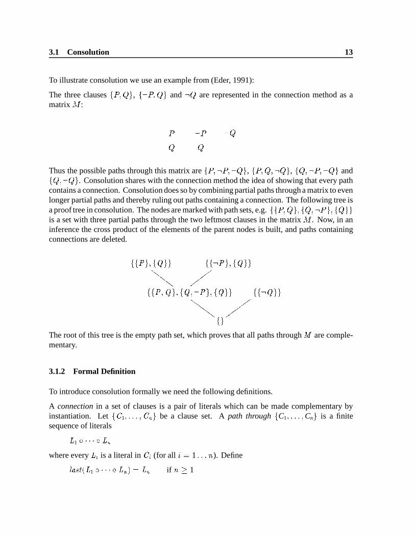
To illustrate consolution we use an example from (Eder, 1991):
The three clauses � � � � , � � � � and � are represented in the connection method as amatrix � :
�
�
�
Thus the possible paths through this matrix are � � � � � , � � � � � � , � � � � � � and� � � � � . Consolution shares with the connection method the idea of showing that every pathcontains a connection. Consolution does so by combining partial paths through a matrix to evenlonger partial paths and thereby ruling out paths containing a connection. The following tree isa proof tree in consolution. The nodes are marked with path sets, e.g. � � � � � � � � � � � � � � �is a set with three partial paths through the two leftmost clauses in the matrix � . Now, in aninference the cross product of the elements of the parent nodes is built, and paths containingconnections are deleted.
� � � � � � � � � � � � � � � � � �
� � � � � � � � � � � � � � � � � � � � � �
� �
� � � � � � � � � � � � � �
� � � � � � � � � � � � � � � �
The root of this tree is the empty path set, which proves that all paths through � are comple-mentary.
3.1.2 Formal Definition
To introduce consolution formally we need the following definitions.
A connection in a set of clauses is a pair of literals which can be made complementary byinstantiation. Let � � 1
� � � � be a clause set. A path through � C1� � Cn
� is a finitesequence of literals
�1 � � �
where every� �
is a literal in � �(for all � � 1 � ). Define
� � � � �1 � � � � � � if � � 1

3.1 Consolution 14
and � � � � � �1 � � � � � �
1 � � � � 1 if � � 1
A path � � �1 � � � immediately extends to a path q iff � � � iff
� � � � 0 � � � � � : � � �1 � � � � � � � � � �
1 � � � For the transitive closure we say that a path � extends to a path q iff � � � � . The partial order� on paths is defined as
� � � iff � � � or else � � � �A path set is a finite multiset of paths. Multisets are like sets, but allow multiple occurrencesof identical elements. Formally, a multiset can be introduced as a function over a certaindomain that maps every element of the domain to a natural number. For convenience we willuse set-notations. For example the set for which � � � 3 and � � 1 and � � � 0 forall other values can be written as � � � � � � � � . As operators for multisets we will use the usualset operators with the obvious intended meaning.
In (Eder, 1991) paths are simply sets and thus the above operations� � � �
,
� � � � �and extension
are unnecessary or rather their effect can be achieved by the usual set operations. Furthermore,the original calculus computes with sets of paths instead of multisets. In (Baumgartner andFurbach, 1992) we argue that our modified calculus is the appropriate formal base for expressingother calculi. Since the arguments given for the modifications carry over to the theory case, werefer the reader to (Baumgartner and Furbach, 1992) for that discussion. The next definitionsare adaptions of the ones in (Eder, 1991) towards our data structures.
If � is a clause � � � �1� � � � then the path set of C is given by the path set� � � �
1� � � �
The product pq of two paths � and � is the path � � � . The product� �
of two path sets�
and�
is defined as� � � � � � � � � �and � � � �
For ease of notation we write � �as an abbreviation for � � � �
.
In the sequel we are also concerned with trees, whose nodes are labelled with literals, exceptfor the root which remains unlabelled. Such trees can be conveniently represented by pathsets by simply taking the sequence of the labels
�1� � � of a branch in the tree as a path�
1 � � � in the corresponding path set. Then the� � � �
operation of above denotes the leafof a branch. This representation is not into: although every such tree can be represented as apath set, there are path sets that may stem from non-isomorphic trees.
In order to define the model elimination and matrix calculi later in this section, we have tointroduce ferns, which are trees whose shape is pictorially as follows:

3.1 Consolution 15
� 11 �
1 � �1
1
� 12 �
2 � �2
2
...
� 1 � � � �
� � � � � � � � � � � � � � � � � � � � � � � � � � � � � �
� � � � � � � � � � � � � � � � � � � � � � � � � � � �
� � � � � � � � � � � � � � � � � � � � � � � � � � � � � �
More formally, a fern F of C1� � Cn with trunk L1 � � Ln is the smallest path set
�satisfying
the following conditions:
1. � �is a clause containing the literal
� �, for all � � 1 � .
2.�
1 � � � � �
3.�
1 � � � � � 1 � � � �, for all � � 1 � , for all
� � � � � � � � �The following concepts will be used in the inference rule below:
Definition 3.1 (Spanning MGU) A substitution � is a spanning MGU for a path set Q iff � isa most general substitution such that every element in Q� contains syntactical complementaryliterals. �Definition 3.2 (Shorteningof paths) A path set
�is obtained from a path set
�by shortening
of paths if there is a surjective mapping f :� � �
such that f p � � p holds for all p � �. �
Definition 3.3 (Simplification) A path set is obtained from a path set�
by simplificationiff
A) there exists a spanning MGU � for some subset Q P, and
B)� B is obtained from
� � by deleting zero or more paths containing complementaryliterals, and
C)� C is obtained from
� B by shortening of zero or more paths, and
D) is obtained from� C in the following way: for every path p � � C zero or more, but
not all paths are deleted that are equal to p as a set of literals.
3.1 Consolution 16
�The motivation for the term “equal as a set of literals” in item D comes from the desire tosimulate the behaviour of sets in Eder’s original consolution. See (Baumgartner and Furbach,1992) for details.
Definition 3.4 (Consolution inference) (Sequence Consolution) The inference rule sequenceconsolution is defined as follows � �
if there exists a variant
� �
of�
which does not have variables in common with�
such that is obtained from
� � �
by simplification. is called a sequence consolvent of�
and�
.
A derivation of a matrix M is a finite sequence � 0� � �
n� of path sets such that the following
conditions hold:
1. For all k � 1 � � n, the set�
k
(a) is a path set�
C of a clause C � M, or
(b) is a consolvent of�
i and a new variant of�
j for some i � j � k.
2.�
n � � �In order to express linear calculi, such as model elimination a slightly modified definition isnecessary. Thus, a linear derivation of a matrix M is a finite sequence � 0
� � �n� of path
sets such that the following conditions hold:
1.�
0 is a path set�
C of a clause C � M.
2. For all k � 1 � � n, the set�
k is a consolvent of�
k � 1 and a new variant of a path set�C of a clause C � M.
3.�
n � � ��
We will not give an example of consolution here, because it would be subsumed by the theoryconsolution examples presented below. Instead we conclude non-theory consolution with thefollowing theorem.
Theorem 3.1 (Soundness and completeness of consolution) (Eder, 1991) A formula in dis-junctive normal form is valid if and only if there is a derivation of its matrix by consolution.
Together with a theorem from (Baumgartner and Furbach, 1992) which states that everyconsolution derivation can be stepwisely simulated by a sequence consolution derivation, thecompleteness of sequence consolution follows.
3.2 Theory Consolution 17
3.2 Theory Consolution
As motivated in the introduction we take apart the knowledge of the domain (i.e. the theory)from the program clauses. Formally, a theory is a satisfiable set of universally quantifiedformulas.
A�
-interpretation is an interpretation satisfying the theory�
. A�
-interpretation� �
-satisfiesa clause set � iff
�simultaneously assigns true to all ground instances of the clauses in � .�
-(un-)satisfiability and�
-validity of clause sets are defined on top of this notion as usual.
The restriction to universally quantified theories, shortly universal theories, is necessary bec-ause precisely for those theories a Herbrand theorem of the following form holds (Petermann,1991b).
Theorem 3.2 A clause set M is�
-unsatisfiable if and only if there is a finite set of groundinstances of clauses from M which is
�-unsatisfiable.
Similar to the non-theory case a Herbrand theorem of this form is the basis for any completenessproof for a calculus which relies on the co-operation of foreground and background reasoning.The restriction is not serious in principle because every theory may be substituted by anequivalent universal theory. However, equivalent means here equivalence with respect totheory-satisfiability and up to the enrichment of the signature by Skolem functions.
3.2.1 The Interface Between General and Dedicated Reasoner
In the present subsection we define the interface between the foreground reasoner, consolution,and the background reasoner. This interface is constituted by three notions. Firstly, we haveto generalize the concept of “complementary pair of literals” to the theory case. Unlike in thenon-theory case, there is no general syntactic characterization in the theory case. Thereforewe will give a semantic pendant which is that of a “theory complementary set of literals”.Secondly, we have to generalize the notion of “unifier”. The task of the background reasoneris to construct from candidates given by the foreground reasoner “theory complementarysets of literals” which play the role of elementary arguments in the course of the refutation.This construction is carried out by instantiating the candidates. We will call the respectivesubstitutions “theory refuters”. Thirdly, in order to be able to treat partial theory reasoningtoo we introduce the notion of “theory residue”.
Definition 3.5 Let S � � L1� � Ln
� be a literal set. S is called�
-complementary iff theexistentially quantified conjunction
� L1� � Ln
� is�
-unsatisfiable. A�
-complementaryset is called minimal
�-complementary iff every true subset is not
�-complementary. �
Equivalently to this definition it holds that � �1� � � � is
�-complementary iff every ground
instance of�
1� � � is
�-unsatisfiable iff the universally quantified disjunction � �
1�

3.2 Theory Consolution 18
� � � is�
-valid.
There is a subtle difference between the�
-complementary of a literal set and its�
-unsatisfiability,when read as a set of unit clauses, i.e. if the variables were � -quantified. These notions are thesame only for ground sets. Consider, for example, a language with at least two constant sym-bols
�and and the “empty” theory � . Then � � � � � � � � � � � is, when read as a clause set,
� -unsatisfiable, but � is not � -complementary, because the conjunction� � � � � � � � � � � �
is not � -valid (because the interpretation with� � � � � �
�� � � �
and� � � � � � � � �
is amodel). However, when applying the substitution � � � � � � � to � the resulting set � � is� -complementary.
The importance of “complementary” arises from its application in inference rules, such asresolution, which for soundness reasons have to be built on top of complementarism. Sincewe deal with theory inference rules, we had to extend the usual notion of “complementarism”to “
�-complementarism”. As a further example consider the theory � of equality (section
4). Then � � � � � � � � �
� � � � �
��
� � � � � is � -unsatisfiable but not � -complementary.However after application of the substitution � � � � � � � � � � � , the set � � is � -complementary. Such substitutions will be called refuters. As with non-theory consolution,the theory consolution derivations should be computed at a most general level; this is achievedby most general refuters. More formally we define:
Definition 3.6 A substitution � is a�
-refuter for S iff S� is�
-complementary. Conversely, Sis called
�-refutable iff a
�-refuter exists for it. If S� is minimal
�-complementary then S is
also called minimal�
-refutable by � . A set of substitutions is a complete set of�
-refuters forS (or short: CSR� S � ) iff
1. for all � � CSR S � : � is a�
-refuter for S (Correctness)
2. for all�
-refuters � for S:there is a � � CSR S � and a substitution � � such that � �var S � � � � � � �var S �(Completeness)
�A “partial” variant of
�-refuters is as follows:
Definition 3.7 A pair � � R � , where � is a substitution and R is a literal, is a�
-residue of S iffS� � � R� is minimal
�-complementary. �
The prefix “�
-” is often omitted in the sequel.
In this context it might be interesting to know that our notion of theory refuter generalizesthe notion of rigid E-unifier (Gallier et al., 1990) to more general theories than equality (see(Burckert, 1990a) for a proof). A dual notion, “unifier with respect to
�-complementary literal
sets”, has been studied within an affirmative setting (Petermann, 1991b). Constraint theories,equational theories and simple taxonomic theories have been discussed there as special cases.
3.2 Theory Consolution 19
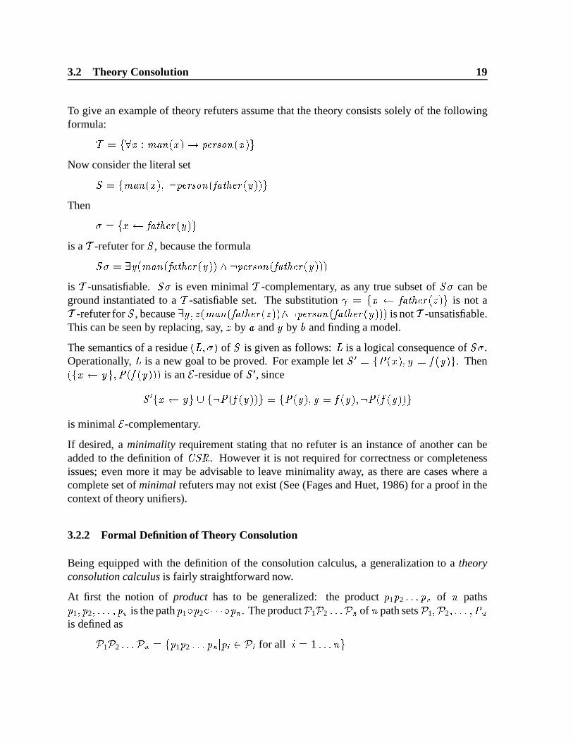
To give an example of theory refuters assume that the theory consists solely of the followingformula:
� � � � � : �� � � � � � � � � � � � � �
Now consider the literal set
� � � �� � � � � � � � � � �
�� � � � � � � � �
Then
� � � � ��
� � � � � � � �is a
�-refuter for � , because the formula
� � � � � �� �
�� � � � � � � � � � � � � � �
�� � � � � � � � �
is�
-unsatisfiable. � � is even minimal�
-complementary, as any true subset of � � can beground instantiated to a
�-satisfiable set. The substitution � � � � �
�� � � � � � � � is not a�
-refuter for � , because� � � � �
� � �
� � � � � � � � � � � � � � � �
� � � � � � � � � is not�
-unsatisfiable.This can be seen by replacing, say, � by
�and � by and finding a model.
The semantics of a residue � � � � of � is given as follows:�
is a logical consequence of � � .Operationally,
�is a new goal to be proved. For example let � � � � � � � � � �
� � � � . Then
� � � � � � � �
� � � � is an � -residue of � � , since
� � � � � � � � � � �
� � � � � � � � � � � �
� � � � �
� � � � �
is minimal � -complementary.
If desired, a minimality requirement stating that no refuter is an instance of another can beadded to the definition of � � � . However it is not required for correctness or completenessissues; even more it may be advisable to leave minimality away, as there are cases where acomplete set of minimal refuters may not exist (See (Fages and Huet, 1986) for a proof in thecontext of theory unifiers).
3.2.2 Formal Definition of Theory Consolution
Being equipped with the definition of the consolution calculus, a generalization to a theoryconsolution calculus is fairly straightforward now.
At first the notion of product has to be generalized: the product � 1 � 2 � of � paths� 1
� � 2� � � is the path � 1 � � 2 � � � . The product
�1�
2 � of � path sets
�1� �
2� � �
is defined as�1�
2 � � � � 1� 2
� � � � � � �for all � � 1 � �
3.2 Theory Consolution 20
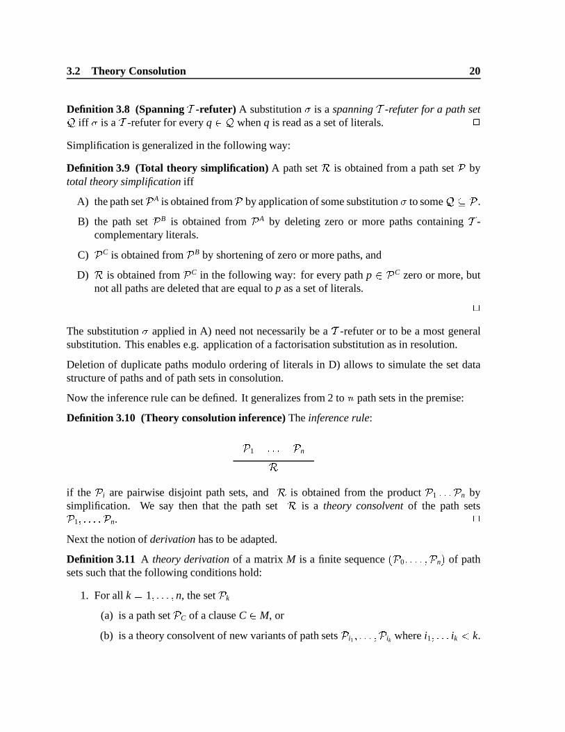
Definition 3.8 (Spanning�
-refuter) A substitution � is a spanning�
-refuter for a path set�iff � is a
�-refuter for every q � �
when q is read as a set of literals. �Simplification is generalized in the following way:
Definition 3.9 (Total theory simplification) A path set is obtained from a path set�
bytotal theory simplification iff
A) the path set� A is obtained from
�by application of some substitution � to some
� �.
B) the path set� B is obtained from
� A by deleting zero or more paths containing�
-complementary literals.
C)� C is obtained from
� B by shortening of zero or more paths, and
D) is obtained from� C in the following way: for every path p � � C zero or more, but
not all paths are deleted that are equal to p as a set of literals.
�The substitution � applied in A) need not necessarily be a
�-refuter or to be a most general
substitution. This enables e.g. application of a factorisation substitution as in resolution.
Deletion of duplicate paths modulo ordering of literals in D) allows to simulate the set datastructure of paths and of path sets in consolution.
Now the inference rule can be defined. It generalizes from 2 to � path sets in the premise:
Definition 3.10 (Theory consolution inference) The inference rule:
�1
�n
if the
�i are pairwise disjoint path sets, and is obtained from the product
�1
�n by
simplification. We say then that the path set is a theory consolvent of the path sets�1� � �
n. �Next the notion of derivation has to be adapted.
Definition 3.11 A theory derivation of a matrix M is a finite sequence � 0� � �
n� of path
sets such that the following conditions hold:
1. For all k � 1 � � n, the set�
k
(a) is a path set�
C of a clause C � M, or
(b) is a theory consolvent of new variants of path sets�
i1� � �
ik where i1� ik
� k.
3.2 Theory Consolution 21
2.�
n � � �A linear theory derivation of a matrix M is a finite sequence � 0
� � �n� of path sets such
that the following conditions hold:
1.�
0 is a path set of a clause C � M.
2. For all k � 1 � � n, the set�
k is a theory consolvent of�
k � 1 and new variants of pathsets
�C1
� � �Cn where the Ci (for i � 1 n) are clauses in M.
3.�
n � � ��
It should have become clear from the preceding definitions that consolution has some openparameters (the commitment to the derivation strategy, and the simplification). Thus onecannot speak of the consolution calculus. Instead consolution should be interpreted as amethod that can be instantiated to several calculi. This will be done in the following sectionsin a goal-oriented way.
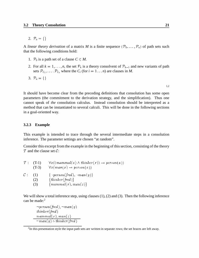
3.2.3 Example
This example is intended to trace through the several intermediate steps in a consolutioninference. The parameter settings are chosen “at random”.
Consider this excerpt from the example in the beginning of this section, consisting of the theory�and the clause set
�:
�: (T-1) � � �
�� �
� � � � � � � � � � � � � � � � � � � � � � � � �(T-3) � � �
� � � � � � � � � � � � � ��
: (1) � � � � � � � � � � � � � �
� � � � �(2) � � � � � � � �
� � � � � �(3) � �
�� �
� � � � � �� � � � �
We will show a total inference step, using clauses (1), (2) and (3). Then the following inferencecan be made:2
� � � � � � � � � � � � �
� � � �� � � � � � � � � � � �
��� �
� � � � � �� � � �
�� � � � � � � � � � � �
� � � � �2In this presentation style the input path sets are written in separate rows; the set braces are left away.
3.3 Partial Theory Consolution 22
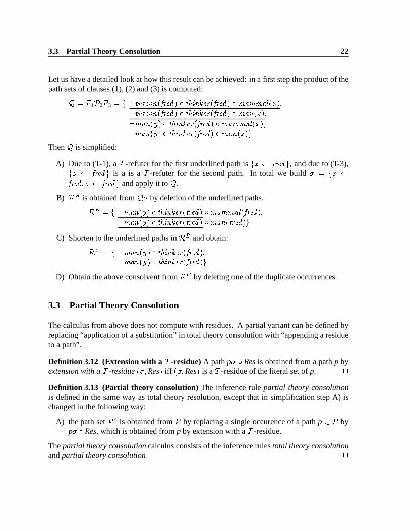
Let us have a detailed look at how this result can be achieved: in a first step the product of thepath sets of clauses (1), (2) and (3) is computed:� � �
1�
2�
3 � � � � � � � � � � � � � � � � � � � � �
� � � � � � ��� �
� � � � � � � � � � �
� � � � � � � � � � � � � � � � � � � �
� � � � � �
� � � � � � � � � � � � � � � � � � �
�� �
� � � � � �
� � � � � � � � � � � � � � � � � � �
� � � � �Then
�is simplified:
A) Due to (T-1), a�
-refuter for the first underlined path is � � �� � � � � , and due to (T-3),
� � �� � � � � is a is a
�-refuter for the second path. In total we build � � � � �� � � � � � �
� � � � � and apply it to�
.
B) � is obtained from� � by deletion of the underlined paths.
� � � �� � � � � � � � � � � �
� � � � � � ��� �
� � � � � � � �
�� � � � � � � � � � � �
� � � � � � �� �
� � � � � �C) Shorten to the underlined paths in � and obtain:
� � �� � � � � � � � � � � �
� � � � � � �
� � � � � � � � � � � � � � � � � �
D) Obtain the above consolvent from
by deleting one of the duplicate occurrences.
3.3 Partial Theory Consolution
The calculus from above does not compute with residues. A partial variant can be defined byreplacing “application of a substitution” in total theory consolution with “appending a residueto a path”.
Definition 3.12 (Extension with a�
-residue) A path p� � Res is obtained from a path p byextension with a
�-residue � � Res � iff � � Res � is a
�-residue of the literal set of p. �
Definition 3.13 (Partial theory consolution) The inference rule partial theory consolutionis defined in the same way as total theory resolution, except that in simplification step A) ischanged in the following way:
A) the path set� A is obtained from
�by replacing a single occurence of a path p � �
byp� � Res, which is obtained from p by extension with a
�-residue.
The partial theory consolution calculus consists of the inference rules total theory consolutionand partial theory consolution �
3.3 Partial Theory Consolution 23
In (Stickel, 1985) residues are introduce on the ground level in a dual way and more generallyas a set of literals instead of a single literal: a set � �
1� � � � � is a
�-residue of a formula
� iff � � �1
� � � � is�
-complementary. Equivalently, this means that the disjunction�1
� � � � is a logical�
-consequence of � . Since this generalisation is straightforwardwe have omitted it for the sake of simplicity.
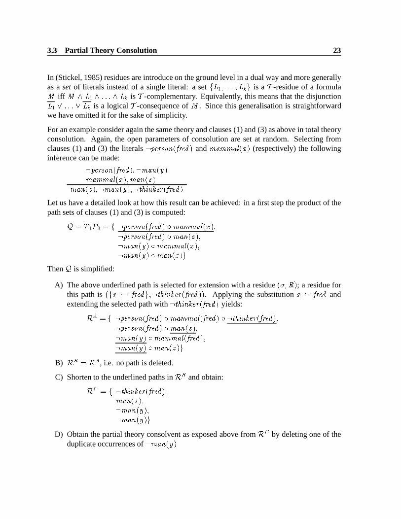
For an example consider again the same theory and clauses (1) and (3) as above in total theoryconsolution. Again, the open parameters of consolution are set at random. Selecting fromclauses (1) and (3) the literals � � � � � �
� � � � � and ��� �
� � � � (respectively) the followinginference can be made:
� � � � � � � � � � � � �
� � � ��
�� �
� � � � � �� � � �
�� � � � � �
� � � � � � � � � � � � � � � � �
Let us have a detailed look at how this result can be achieved: in a first step the product of thepath sets of clauses (1) and (3) is computed:� � �
1�
3 � � � � � � � � � � � � � � �
�� �
� � � � � � � � � � �
� � � � � � �� � � � �
�� � � � � �
�� �
� � � � � �
� � � � � �� � � � �
Then�
is simplified:
A) The above underlined path is selected for extension with a residue � � � � ; a residue forthis path is � � �
� � � � � � � � � � � � � � � � � � � . Applying the substitution � �
� � � �and
extending the selected path with � � � � � � � � � � � � yields:
�
� � � � � � � � � � � � � � �
�� �
� � � � � � � � � � � � � � �
� � � � � � � � � � � �
� � � � � � �� � � � �
�� � � � � �
�� �
� � � � � � � �
�� � � � � �
� � � � �B) � � �
, i.e. no path is deleted.
C) Shorten to the underlined paths in � and obtain:
� � � � � � � � � � � � � � �
�� � � � �
�� � � � �
�� � � � �
D) Obtain the partial theory consolvent as exposed above from
by deleting one of theduplicate occurrences of �
� � � �

3.4 Theory Resolution 24
Now we have defined the formal framework that can be instantiated to the various theorycalculi. Let us quickly summarize what “parameters” have to be instantiated in the theoryconsolution calculus:
� Concerning derivation: The function
�and the commitment to a non-linear or linear
strategy.� Concerning simplification: The parameters of step A (application of a substitution or
extension with a residue), step B (deleting complementary paths), step C (shortening ofpaths) and step D (deleting occurrences).
3.4 Theory Resolution
We assume the reader to be familiar with the resolution calculus and its terminology (see e.g.(Loveland, 1978; Chang and Lee, 1973) for introductory textbooks). First we will explain theoriginal version of theory resolution (Stickel, 1985). Then, after the formal definition basedon theory consolution is given, completeness will be proved.
3.4.1 Informal Explanation
In (Stickel, 1985) several variants of a theory resolution calculus are defined. One of themis called narrow total theory resolution. We will demonstrate a first-order version of thisrule. It takes � clauses as inputs and selects one literal from each of the � clauses such thatthese literals can be instantiated to a theory-complementary set. Then the resolvent is builtas in ordinary resolution by applying the substitution and collecting the rest of the clauses.Thus narrow theory resolution is a straightforward “semantical” generalization of the ordinaryresolution rule.
Example. This is an excerpt from the example in the introduction:
�: (T-1) � � �
�� �
� � � � � � � � � � � � � � � � � � � � � � � � �(T-3) � � �
� � � � � � � � � � � � � ��
: (1) � � � � � � � � � � � � � �
� � � � �(2) � � � � � � � �
� � � � � �(3) � �
�� �
� � � � � �� � � � �
We will show an inference step, using from clauses (1), (2) and (3) the literals � � � � � � � � � � � ,� � � � � � �
� � � � � and ��� �
� � � � (respectively) as a�
-refutable literal set. It can easily be seenthat � � �
� � � � � is a�
-refuter for this set (join the clause form of (T-1) to this set and find

3.4 Theory Resolution 25
a resolution refutation). Hence the following resolvent can be built (the selected literals areunderlined) :
� � � � � � � � � � � � � �
� � � � �� � � � � � � �
� � � � � �� �
�� �
� � � � � �� � � � �
� �� � � � � �
� � � � � with refuter � � �x � fred �
It should be noted that sometimes factorization has to be carried out for completeness reasons.This can either be done by an extra inference rule, or by incorporating factorization into theresolution inference rule. Since factorization is not central for the idea of theory reasoning, wewill skip over it for the moment.
The partial variant of theory resolution is similar to the total theory resolution rule, except thatthe resolvent additionally includes a residue in the resolvent. Stickel’s ground calculus allowsas residues disjunctions � 1
� � � � of literals. The disjunction � � � 1� � � � is a
residue of a conjunction � � � 1� � � � if � implies � . Here we will restrict ourselves to
the important special case where the residue is a single literal � 1. A generalization would bestraightforward if desired.
Example. Using the example of above, we have that
� � �� � � � � � � � � � � � �
� � � � � �is a residue of
� � � � � � � � � � � � � �
�� �
� � � � �which is built from literals in clauses (1) and (3). Thus we arrive at the following partial theoryresolution inference:
� � � � � � � � � � � � � �
� � � � �� �
�� �
� � � � � �� � � � �
� � � � � � � � � � � � � �
� � � � � �� � � � � with residue � �
x � fred � thinker � fred � �Now resolving this resolvent in an ordinary resolution step against (2) we could arrive at thesame clause as in the above total theory step. As a general property one could say that thepurpose of partial theory reasoning is to approximate a total theory reasoning step in a sequenceof partial steps, followed by one single total step.
A problem of Stickel’s original definition is that it allows one to derive many redundant clauses.For example, in the theory of strict orderings from
� � and � � one might infer the residue� � � , but also residues like � � � � � � � , � � � � � � � � � � � � � , . Thus inpractice it is inevitable to seek for suitable restrictions. See again (Stickel, 1985) for a moredetailed discussion how redundant residues can be omitted.
So far we have discussed narrow theory resolution. In (Stickel, 1985) a more general variant

3.4 Theory Resolution 26
called wide theory resolution is defined. It differs from narrow theory resolution in that nolonger are only single literals of the clauses considered in inferences, but instead subclausesare passed to the theory reasoner. This however complicates the theory reasoner, since it mustoperate on clause sets instead of literal sets. Similar to the narrow case, a total and a partialvariant can be defined.
3.4.2 Formal Definition
The total theory resolution inference rule can be defined as an instance of theory consolution.For the total version we need two inference rules: total theory resolution and factorisation.For the former � clauses have to be chosen and they have to be put into a format suitable forthe theory consolution operation. The simplification operation in theory consolution has tobe defined in such a way that the consolvent corresponds precisely to the theory resolvent intheory resolution. More formally we arrive at the following inference rule:
Definition 3.14 (Total theory resolution) The inference rule total theory resolution is definedas follows: � �
L1 � � R1
...� �Ln � � Rn
where
1. � Li� � Ri are pairwise variable disjoint clauses (for i � 1 n � n � 1).
2. � L1� � Ln
� is�
-refutable.
3. The simplification of the product� � � �L1 � � R1 � �
Ln � � Rn
is done in the following way:
A) Q� is obtained from�
by application of the�
-refuter � of � L1� � Ln
� (whichexists by 2.)
B) Delete every path L1 � � Ln� � from
� � and obtain B.
C) C is obtained from B by shortening every path in B according to
f K1 � � Km� � Ki
where i � � 1 � � m � such that Ki�� � L1
� � Ln� �
D) is obtained from C by deleting for every path all its duplicate occurences.
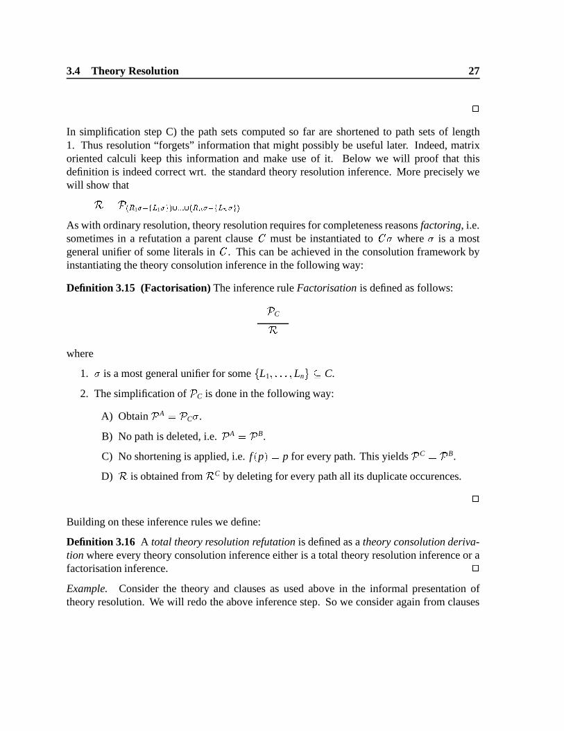
3.4 Theory Resolution 27
�In simplification step C) the path sets computed so far are shortened to path sets of length1. Thus resolution “forgets” information that might possibly be useful later. Indeed, matrixoriented calculi keep this information and make use of it. Below we will proof that thisdefinition is indeed correct wrt. the standard theory resolution inference. More precisely wewill show that
� � � �1� � � �
1 � � � � � � � �� � � � � � � � � � �
As with ordinary resolution, theory resolution requires for completeness reasons factoring, i.e.sometimes in a refutation a parent clause � must be instantiated to � � where � is a mostgeneral unifier of some literals in � . This can be achieved in the consolution framework byinstantiating the theory consolution inference in the following way:
Definition 3.15 (Factorisation) The inference rule Factorisation is defined as follows:
�C
where
1. � is a most general unifier for some � L1� � Ln
� C.
2. The simplification of�
C is done in the following way:
A) Obtain� A � �
C � .
B) No path is deleted, i.e.� A � � B.
C) No shortening is applied, i.e. f p � � p for every path. This yields� C � � B.
D) is obtained from C by deleting for every path all its duplicate occurences.
�Building on these inference rules we define:
Definition 3.16 A total theory resolution refutation is defined as a theory consolution deriva-tion where every theory consolution inference either is a total theory resolution inference or afactorisation inference. �Example. Consider the theory and clauses as used above in the informal presentation oftheory resolution. We will redo the above inference step. So we consider again from clauses

3.4 Theory Resolution 28
(1), (2) and (3) the literals � � � � � � � � � � � , � � � � � � �
� � � � � and ��� �
� � � � (respectively) as�-complementary literal set. Then the following inference can be made:
� � � � � � � � � � � � �
� � � �� � � � � � � � � � � �
��� �
� � � � � �� � � �
�� � � � � �
� � � �Observe that the resulting path set encodes the same clause as in the example of the aboveinformal presentation. Let us have a detailed look at how this result can be achieved: in a firststep the product of the path sets is computed:� � �
1�
2�
3 � � � � � � � � � � � � � � � � � � � � �
� � � � � � ��� �
� � � � � � � � � � �
� � � � � � � � � � � � � � � � � � � �
� � � � � �
� � � � � � � � � � � � � � � � � � �
�� �
� � � � � �
� � � � � � � � � � � � � � � � � � �
� � � � �Then
�is simplified:
A) The�
-refuter � � �� � � � � for the literals in the underlined path
� � � � � � � � � � � � � � � � � � �
� � � � � � ��� �
� � � � � �is applied to
�.
B) � is obtained from� � by deletion of � �
� � � � � � � � � � � � � � � � � � � � � �
� � � � � � �� � � � �
�� � � � � � � � � � � �
� � � � � � ��� �
� � � � � � � �
�� � � � � � � � � � � �
� � � � � � �� � � � �
�
C) Shorten to the underlined paths in � and obtain, modulo multiplicity of paths:
� � �� � � � �
�� � � � �
�� � � � �
It can be verified that this shortening is indeed achieved by the specification of thedefinition.
D) Obtain � from
by deleting the underlined path.
The partial variant of theory resolution is obtained in much the same way:
Definition 3.17 (Partial theory resolution) The inference rule partial theory resolution isdefined as follows:

3.4 Theory Resolution 29
�R1 �
�L1 �
...�Rn �
�Ln �
where
1. � Li� � Ri are pairwise variable disjoint clauses (for i � 1 n).
2. There is a most general residue � � Res � for � L1� � Ln
� .
3. The simplification of the product� � � �L1 � � R1
� � �Ln � � Rn
�is done in the following way:
A)�
has the form� � � L1 � � Ln� � � �
Obtain
� L1 � � Ln� � � Res � � � � �
from�
by extension with a�
-residue � � Res � for L1 � � Ln (which exists by 2).
B) Let B � A, i.e. do not delete any complementary path.
C) C is obtained from B by shortening every path in B according to
f K1 � � Km� � Ki
where i � � 1 � � m � such that Ki�� � L1
� � Ln� �
D) is obtained from C by deleting for every path all its duplicate occurences.
A partial theory resolution refutation is defined as a theory consolution derivation where everytheory consolution inference is an “total theory resolution” or “partial theory resolution” �By shortening the path �
1 � � � � � � � �� �
to the path �� �
(due to simplification step C) atleat one occurence of such a path must be contained in the result) and shortening the other pathsto
� �1 � � � � �
� � � as in total theory resolution, and finally “collapsing” all multiple occurrencesof paths into one occurrence, we obtain precisely the path set corresponding to the resolventof the
traditional inference rule.
3.4 Theory Resolution 30
Example. Consider again the same theory and clauses as above. We will show a partial theoryresolution step, using from clauses (1) and (3) the literals � � � � � �
� � � � � and ��� �
� � � �(respectively) to derive the residue � � � � � � �
� � � � � . Then the following inference can be made:
� � � � � � � � � � � � �
� � � ��
�� �
� � � � � �� � � �
� � � � � � � � � � � � � �
� � � � � �� � � �
Observe again that the resulting path set encodes the same clause as in the example of theabove informal presentation. Let us have a detailed look at how this result can be achieved: ina first step the product of the path sets is computed:� � � � � � � � �
� � � � � � ��� �
� � � � � � � � � � �
� � � � � � �� � � � �
�� � � � � �
�� �
� � � � � �
� � � � � �� � � � �
Then�
is simplified:
A) The above underlined path
� � � � � � � � � � � � � � �
�� �
� � � �is selected for finding a most general residue; a most general residue for � is
�� � � � � �
� � � � � � � � � � � � � � � � � � �
So we obtain by replacement of � � with
� � � � � � � � � � � � � � �
�� �
� � � � � � � � � � � � � � �
� � � � �the path set
�
� � � � � � � � � � � � � � �
�� �
� � � � � � � � � � � � � � �
� � � � � � � � � � � �
� � � � � � �� � � � �
�� � � � � �
�� �
� � � � � � � �
�� � � � � �
� � � � �B) Let � � �
, i.e. do not delete any complementary path.
C) The result of the inference rule must be the path set corresponding to the clause � � � � � �
� � � � � � �� � � � � �
� � � � . This path set, modulo multiplicity of paths,is obtained from � by shortening the paths such that the underlined subpaths in B) arekept. This results in the path set
� � � � � � � � � � � � � � � �
� � � � � �� � � � � �
� � � � �D) delete one occurrence of �
� � � � in
to obtain .

3.4 Theory Resolution 31
3.4.3 Completeness
Completeness of the consolution-style total theory resolution calculus is obtained by simulatinganother theory resolution resolution calculus known to be complete. This strategy was alsoused for the non-theory case in (Eder, 1991). As a preliminary we cite from (Baumgartner,1992b) a theory resolution calculus. The calculus defined there takes advantage of orderingrestrictions which we will omit below. This is legal for our purposes, since an ordered refutationalways is an unordered one as well. Thus, the completeness result for the ordered calculus asdeveloped in (Baumgartner, 1992b) holds as well for the unordered case.
Definition 3.18 ((Baumgartner, 1992b), Clausal Theory Resolution Calculus) The infe-rence rules of the clausal theory resolution (CTR) calculus are defined as follows:
Clausal factoring:C
C��
if � is a most general (syntactical) unifierfor some � L1
� � Ln� C
Clausal theory resolution:C1
Cn
C1 � � � L1� � � � � Cn � � � Ln� � ��
if � is a�
-refuter for � L1� � Ln
� forsome L1 � C1
� � Ln � Cn
In these inference rules, the Li’s are called the selected literals. Let M be a clause set. ACTR-derivation of Cn from M is a sequence C1
� � Cn where each Ci � M or is obtained byan application of the above inference rules to k variable disjoint copies of clauses Cj1
Cjk
where j1� i � � jk
� i. A refutation of M is a derivation of the empty clause. �This calculus is complete:
Theorem 3.3 ((Baumgartner, 1992b), Completeness of clausal theory resolution) Let�
be a theory and M be a�
-unsatisfiable clause set. Then there exists an CTR-refutation of M.
Building on this, we can prove the consolution-style version complete:
Theorem 3.4 (Completeness of Total Theory Resolution) Let�
be a theory and M be a�-unsatisfiable clause set. Then there exists a total theory resolution refutation of M.
Proof. The proof is in analogy to the corresponding theorem for the non-theory case in(Eder, 1991). By the previous theorem it suffices to show that every clausal theory resolutionrefutation can be simulated by step within total theory resolution.
Since the definitions of derivation are the same in total theory resolution and clausal theoryresolution the only non-trivial task is to show how to simulate the inference rules:
3.4 Theory Resolution 32
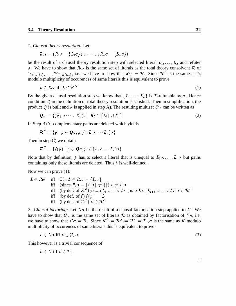
1. Clausal theory resolution: Let
�� � � � 1 � � � �
1� � � � � � � � � � � � �be the result of a clausal theory resolution step with selected literal
�1� � � and refuter
� . We have to show that �� �
is the same set of literals as the total theory consolvent of� �1 �
� �1 � � � � � � �
� � � � , i.e. we have to show that �� � � . Since
is the same as
modulo multiplicity of occurences of same literals this is equivalent to prove� � �
� �iff
� �
(1)
By the given clausal resolution step we know that � �1� � � � is
�-refutable by � . Hence
condition 2) in the definition of total theory resolution is satisfied. Then in simplification, theproduct � is built and � is applied in step A). The resulting multiset � � can be written as
� � � � � 1 � � � � � � �� � � � � � � � � � (2)
In Step B)�
-complementary paths are deleted which yields
� � � � � � � � � � � �� �
1 � � � � �Then in step C) we obtain
� ��
� � � � � � � � � �� �
1 � � � � �Note that by definition,
�has to select a literal that is unequal to
�1 � � � � � but paths
containing only these literals are deleted. Thus
�is well-defined.
Now we can prove (1):� � �
� �iff
� � :� � � � � � � � � � �
iff (since � � � � � � � � � �� � � )
� �� � � �
iff (by def. of � ) � � � �1 � � � � � 1
� � � � � � � �1 � � � � � � �
iff (by def. of
�)
� � � � � �
iff (by def. of
)� �
2. Clausal factoring: Let � � be the result of a clausal factorisation step applied to � . Wehave to show that � � is the same set of literals as obtained by factorisation of
� , i.e.
we have to show that � � � . Since
� � � �
� � � is the same as modulomultiplicity of occurences of same literals this is equivalent to prove
� � � � iff� � � � (3)
This however is a trivial consequence of� � � iff
� � � �
3.4 Theory Resolution 33
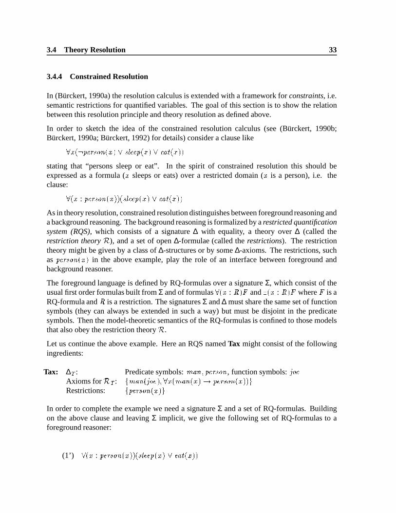
3.4.4 Constrained Resolution
In (Burckert, 1990a) the resolution calculus is extended with a framework for constraints, i.e.semantic restrictions for quantified variables. The goal of this section is to show the relationbetween this resolution principle and theory resolution as defined above.
In order to sketch the idea of the constrained resolution calculus (see (Burckert, 1990b;Burckert, 1990a; Burckert, 1992) for details) consider a clause like
� � � � � � � � � � � � � � � � � � � � � � � � �stating that “persons sleep or eat”. In the spirit of constrained resolution this should beexpressed as a formula ( � sleeps or eats) over a restricted domain ( � is a person), i.e. theclause:
� � : � � � � � � � � � � � � � � � � � � � � � � �As in theory resolution, constrained resolution distinguishes between foreground reasoning anda background reasoning. The background reasoning is formalized by a restricted quantificationsystem (RQS), which consists of a signature ∆ with equality, a theory over ∆ (called therestriction theory ), and a set of open ∆-formulae (called the restrictions). The restrictiontheory might be given by a class of ∆-structures or by some ∆-axioms. The restrictions, suchas � � � � � � � � in the above example, play the role of an interface between foreground andbackground reasoner.
The foreground language is defined by RQ-formulas over a signature Σ, which consist of theusual first order formulas built from Σ and of formulas � � : � � �
and� � : � � �
where�
is aRQ-formula and � is a restriction. The signatures Σ and ∆ must share the same set of functionsymbols (they can always be extended in such a way) but must be disjoint in the predicatesymbols. Then the model-theoretic semantics of the RQ-formulas is confined to those modelsthat also obey the restriction theory .
Let us continue the above example. Here an RQS named Tax might consist of the followingingredients:
Tax: ∆ � : Predicate symbols: �� � � � � � � � � , function symbols:
� � �Axioms for � : � �
� � � � � � � � � �� � � � � � � � � � � � � � �
Restrictions: � � � � � � � � � �
In order to complete the example we need a signature Σ and a set of RQ-formulas. Buildingon the above clause and leaving Σ implicit, we give the following set of RQ-formulas to aforeground reasoner:
(1’) � � : � � � � � � � � � � � � � � � � � � � � � � �
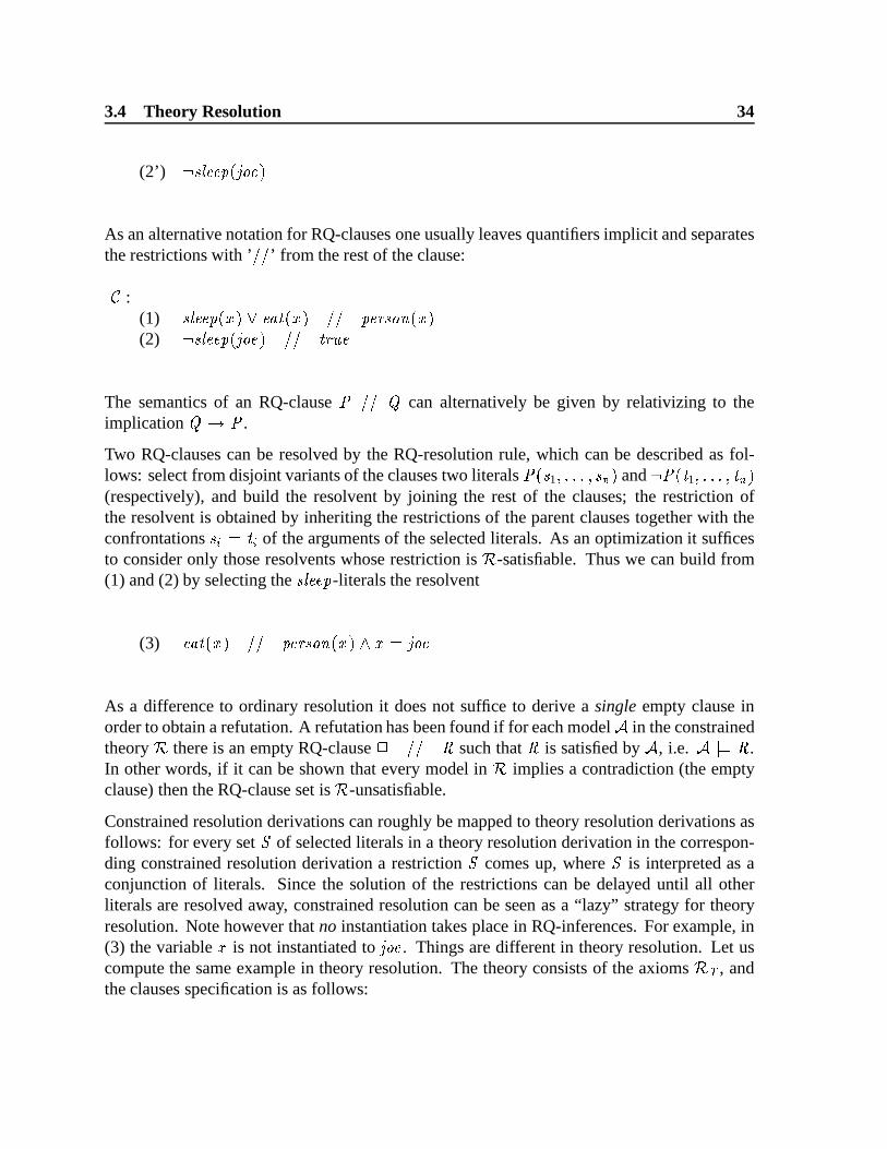
3.4 Theory Resolution 34
(2’) � � � � � � � � �
As an alternative notation for RQ-clauses one usually leaves quantifiers implicit and separatesthe restrictions with ’ � � ’ from the rest of the clause:
�:
(1)� � � � � � � � � � � � � � � � � � � � � � �
(2) � � � � � � � � � � � � � � �
The semantics of an RQ-clause � � � � can alternatively be given by relativizing to theimplication � � � .
Two RQ-clauses can be resolved by the RQ-resolution rule, which can be described as fol-lows: select from disjoint variants of the clauses two literals � �
1� � � � and � �
1� � � �
(respectively), and build the resolvent by joining the rest of the clauses; the restriction ofthe resolvent is obtained by inheriting the restrictions of the parent clauses together with theconfrontations
� � � � �of the arguments of the selected literals. As an optimization it suffices
to consider only those resolvents whose restriction is -satisfiable. Thus we can build from(1) and (2) by selecting the
� � � � � -literals the resolvent
(3)� � � � � � � � � � � � � � � � � � � � �
As a difference to ordinary resolution it does not suffice to derive a single empty clause inorder to obtain a refutation. A refutation has been found if for each model � in the constrainedtheory there is an empty RQ-clause � � � � such that � is satisfied by � , i.e. � �� � .In other words, if it can be shown that every model in implies a contradiction (the emptyclause) then the RQ-clause set is -unsatisfiable.
Constrained resolution derivations can roughly be mapped to theory resolution derivations asfollows: for every set � of selected literals in a theory resolution derivation in the correspon-ding constrained resolution derivation a restriction � comes up, where � is interpreted as aconjunction of literals. Since the solution of the restrictions can be delayed until all otherliterals are resolved away, constrained resolution can be seen as a “lazy” strategy for theoryresolution. Note however that no instantiation takes place in RQ-inferences. For example, in(3) the variable � is not instantiated to
� � �. Things are different in theory resolution. Let us
compute the same example in theory resolution. The theory consists of the axioms � , andthe clauses specification is as follows:
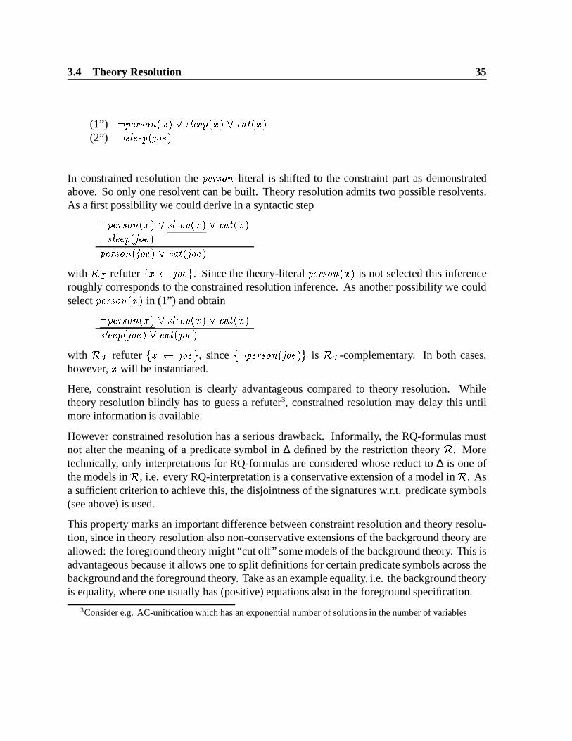
3.4 Theory Resolution 35
(1”) � � � � � � � � � � � � � � � � � � � � � �(2”) � � � � � � � � �
In constrained resolution the � � � � � � -literal is shifted to the constraint part as demonstratedabove. So only one resolvent can be built. Theory resolution admits two possible resolvents.As a first possibility we could derive in a syntactic step
� � � � � � � � � � � � � � � � � � � � � � � � � � � � � � �� � � � � � � � � � � � � � � � � �
with � refuter � � � � � � � . Since the theory-literal � � � � � � � � is not selected this inferenceroughly corresponds to the constrained resolution inference. As another possibility we couldselect � � � � � � � � in (1”) and obtain
� � � � � � � � � � � � � � � � � � � � � �� � � � � � � � � � � � � � � � �
with � refuter � � � � � � � , since � � � � � � � � � � � � is � -complementary. In both cases,however, � will be instantiated.
Here, constraint resolution is clearly advantageous compared to theory resolution. Whiletheory resolution blindly has to guess a refuter3, constrained resolution may delay this untilmore information is available.
However constrained resolution has a serious drawback. Informally, the RQ-formulas mustnot alter the meaning of a predicate symbol in ∆ defined by the restriction theory . Moretechnically, only interpretations for RQ-formulas are considered whose reduct to ∆ is one ofthe models in , i.e. every RQ-interpretation is a conservative extension of a model in . Asa sufficient criterion to achieve this, the disjointness of the signatures w.r.t. predicate symbols(see above) is used.
This property marks an important difference between constraint resolution and theory resolu-tion, since in theory resolution also non-conservative extensions of the background theory areallowed: the foreground theory might “cut off” some models of the background theory. This isadvantageous because it allows one to split definitions for certain predicate symbols across thebackground and the foreground theory. Take as an example equality, i.e. the background theoryis equality, where one usually has (positive) equations also in the foreground specification.
3Consider e.g. AC-unification which has an exponential number of solutions in the number of variables
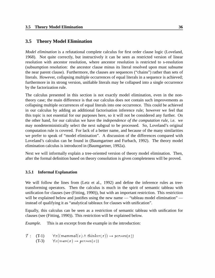
3.5 Theory Model Elimination 36
3.5 Theory Model Elimination
Model elimination is a refutational complete calculus for first order clause logic (Loveland,1968). Not quite correctly, but instructively it can be seen as restricted version of linearresolution with ancestor resolution, where ancestor resolution is restricted to s-resolution(subsumption resolution: the ancestor clause minus its literal resolved upon must subsumethe near parent clause). Furthermore, the clauses are sequences (“chains”) rather than sets ofliterals. However, collapsing multiple occurrences of equal literals in a sequence is achieved;furthermore in its strong version, unifiable literals may be collapsed into a single occurrenceby the factorization rule.
The calculus presented in this section is not exactly model elimination, even in the non-theory case; the main difference is that our calculus does not contain such improvements ascollapsing multiple occurrences of equal literals into one occurrence. This could be achievedin our calculus by adding an additional factorisation inference rule; however we feel thatthis topic is not essential for our purposes here, so it will not be considered any further. Onthe other hand, for our calculus we have the independence of the computation rule, i.e. wemay nondeterministically select the next subgoal to be processed. So, Loveland’s originalcomputation rule is covered. For lack of a better name, and because of the many similaritieswe prefer to speak of “model elimination”. A discussion of the differences compared withLoveland’s calculus can be found in (Baumgartner and Furbach, 1992). The theory modelelimination calculus is introduced in (Baumgartner, 1992a).
Next we will informally explain a tree-oriented version of theory model elimination. Then,after the formal definition based on theory consolution is given completeness will be proved.
3.5.1 Informal Explanation
We will follow the lines from (Letz et al., 1992) and define the inference rules as tree-transforming operators. Then the calculus is much in the spirit of semantic tableau withunification for clauses (see (Fitting, 1990)), but with an important restriction. This restrictionwill be explained below and justifies using the new name — “tableau model elimination” —instead of qualifying it as “analytical tableaux for clauses with unification”.
Equally, this calculus can be seen as a restriction of semantic tableau with unification forclauses (see (Fitting, 1990)). This restriction will be explained below.
Example. This is an excerpt from the example in the introduction:
�: (T-1) � � �
�� �
� � � � � � � � � � � � � � � � � � � � � � � � �(T-3) � � �
� � � � � � � � � � � � � �

3.5 Theory Model Elimination 37
�: (1) � � � � � � �
� � � � � � �� � � � �
(2) � � � � � � � � � � � � � �
(3) � ��� �
� � � � � �� � � � �
Model elimination tries to construct a semantic tableau, where every branch is�
-complementary(“closed”). We have to pick a clause and construct an initial tableau; selecting clause (1) yields:
� � � � � � � � � � � �
� � � ��� � � � � � � �
� ��
��
��
��
We will show a theory extension step, using from the left branch � � � � � � � � � � � and from
clauses (2) and (3) the literals� � � � � � �
� � � � � and ��� �
� � � � (respectively) as a�
-refutableliteral set. It can easily be seen that � � �
� � � � � is a�
-refuter for this set (join the clause formof (T-1) to this set and find a resolution refutation). Hence the tableau can be extended at theleft branch with clauses (2) and (3) in such a way that a branch labelled with the complementaryliteral set comes up:
� � � � � � � � � � � �
� � � �
� � � � � � � � � � � �
��� �
� � � � � � �
��
� � � �
��
��
��
�� �
��
��
��
�
��
��
�� �
��
��
��
�
The path containing the set of�
-unsatisfiable literals is closed, i.e. it is marked with an asterixand the
�-refuter is applied to the whole tree.
Such a closing of a path can also be done by the second inference rule, the reduction step:if a path contains a set of literals that are theory complementary by some
�-refuter � , it
can be closed and the MGR is applied to the entire tree. The branch ending in �� � � � can
be closed in a reduction step, because by (T-3) the literals �� � � � and � � � � � �
� � � � � are�-complementary by
�-refuter � � �
� � � � � .
This process has to be repeated until a tree is derived where all branches are marked with astar. Then a refutation is found.

3.5 Theory Model Elimination 38
3.5.2 Formal Definition
In the formalisation of this calculus we need only one inference rule, namely the extensionrule, because the reduction rule will become an instance of the extension rule:
Definition 3.19 (Total theory model elimination) The inference rule total theory extensionis defined as follows: � � � p ��
R1 ��L1 �
...�Rn �
�Ln �
where
1.� � � p � is a path set.
2. � Li� � Ri are pairwise variable disjoint clauses (for i � 1 n).
3. for some subset q of the literal set of front p � the set q � � last p � � L1� � Ln
� is minimal�-refutable. Let
�be a CSR for that set.
4. The simplification of the product� � � � � p � � � R1 ��L1 � �
Rn ��Ln � �
is done in the following way:
A)� � is obtained from
�by application of a
�-refuter � � �
for � q � L1� � Ln
�(which exists by 2.)
B) Delete p � L1 � � Ln� � from
� � and obtain B.
C) Let � be the fern of L1� R1
� � Ln� Rn with trunk L1 � � Ln. Then obtain C
from B by shortening to the path set that is specified as follows:
C � � � � � � p � � � � L1 � � Ln� � � � �
D) Delete some duplicate occurrences of some paths in C to obtain .
A total model elimination refutation is defined as a linear theory consolution derivation whereevery theory consolution inference is a “total theory model elimination”. �In terms of the traditional calculus, the path set
� � � � � is intended to represent the tableauthat is extended at its branch � . Then the effect of C) is to append to � the fern formed fromthe clauses to extend with. It is due to the design of “derivation” and “simplification” that
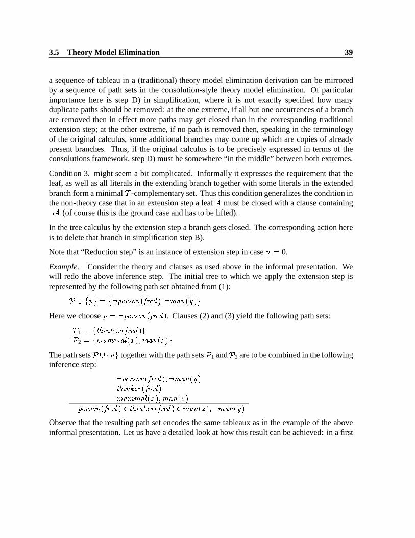
3.5 Theory Model Elimination 39
a sequence of tableau in a (traditional) theory model elimination derivation can be mirroredby a sequence of path sets in the consolution-style theory model elimination. Of particularimportance here is step D) in simplification, where it is not exactly specified how manyduplicate paths should be removed: at the one extreme, if all but one occurrences of a branchare removed then in effect more paths may get closed than in the corresponding traditionalextension step; at the other extreme, if no path is removed then, speaking in the terminologyof the original calculus, some additional branches may come up which are copies of alreadypresent branches. Thus, if the original calculus is to be precisely expressed in terms of theconsolutions framework, step D) must be somewhere “in the middle” between both extremes.
Condition 3. might seem a bit complicated. Informally it expresses the requirement that theleaf, as well as all literals in the extending branch together with some literals in the extendedbranch form a minimal
�-complementary set. Thus this condition generalizes the condition in
the non-theory case that in an extension step a leaf � must be closed with a clause containing � (of course this is the ground case and has to be lifted).
In the tree calculus by the extension step a branch gets closed. The corresponding action hereis to delete that branch in simplification step B).
Note that “Reduction step” is an instance of extension step in case � � 0.
Example. Consider the theory and clauses as used above in the informal presentation. Wewill redo the above inference step. The initial tree to which we apply the extension step isrepresented by the following path set obtained from (1):� � � � � � � � � � � � �
� � � � � � �� � � � �
Here we choose � � � � � � � � � � � � � . Clauses (2) and (3) yield the following path sets:�
1 � � � � � � � � � � � � � � ��
2 � � ��� �
� � � � � �� � � � �
The path sets� � � � � together with the path sets
�1 and
�2 are to be combined in the following
inference step:
� � � � � � � � � � � � �
� � � �� � � � � � � � � � � �
��� �
� � � � � �� � � �
� � � � � � � � � � � � � � � � � � �
� � � � � � �� � � � � �
� � � �Observe that the resulting path set encodes the same tableaux as in the example of the aboveinformal presentation. Let us have a detailed look at how this result can be achieved: in a first

3.5 Theory Model Elimination 40
step the product of the path sets is computed:� � � � � � � � �1�
2 � � � � � � � � � � � � � � � � � � � � �
� � � � � � ��� �
� � � � � � � � � � �
� � � � � � � � � � � � � � � � � � � �
� � � � � �
� � � � � � � � � � � � � � � � � � �
�� �
� � � � � �
� � � � � � � � � � � � � � � � � � �
� � � � �Then
�is simplified:
A) The above underlined path
� � � � � � � � � � � � � � � � � � �
� � � � � � ��� �
� � � � � �is selected for finding a
�-refuter � ; a
�-refuter for this path is � � �
� � � � � .
B) � is obtained from� � by deletion of � �
� � � � � � � � � � � � � � � � � � � � � �
� � � � � � �� � � � �
�� � � � � � � � � � � �
� � � � � � ��� �
� � � � � � � �
�� � � � � � � � � � � �
� � � � � � �� � � � �
C) Shorten to the underlined paths in � and obtain, modulo multiplicity of paths:
� � � � � � � � � � � � � � � � � � � � �
� � � � � � �� � � � �
�� � � � �
�� � � � �
It can be verified that this shortening is indeed achieved by the specification of thedefinition.
D) Obtain � from
by deleting the underlined path.
The partial variant of theory model elimination can be defined in much the same way as totaltheory resolution is modified to partial theory resolution. This is omitted here.
3.5.3 Completeness
Completeness of the consolution-style theory model elimination is obtained by simulatinganother theory model elimination calculus known to be complete, namely the calculus from(Baumgartner, 1992a). To distinguish it from the above introduced model elimination, we willcall this calculus tableaux model elimination.

3.5 Theory Model Elimination 41
Tableaux Model Elimination
In (Baumgartner, 1992a) tableaux are introduced as so called literal trees, i.e. multiset ofbranches, which form a tree, the nodes of which are labelled with literals. Note that withoutthis distinction between nodes and their labels, we get our multisets of paths. A literal tree � �is obtained from a literal tree � by extension with a clause L1
� � Ln at a branch b iff
� � � � � � � � � � � � � � � 1 � and� �
is labelled with� � �
In this case we also say that � � contains a clause�
1� � � � rooted at .
The term “to close a branch” means to attach an additional label “� ” to its leaf in order toindicate that the branch is proved to be
�-complementary. A branch is open iff it is not
labelled in that way.
Definition 3.20 (Total Theory Tableau Model Elimination) Let M be a clause set and�
bea theory. An initial model elimination tableau for M with top clause C is a literal tree thatresults from extending the empty tree (the tree that contains only the empty branch) with theclause C.
A model elimination tableau (ME tableau) for M is either an initial ME tableau or a literal treeobtained by a single application of one of the following inference rules to a ME tableau T:
Extension step: Let b � L1 � � Lk � 1 � Lk be an open branch in T . Suppose there exist newvariants Ci � K1
i� � Kmi
i (i � 1 n) of clauses in M. These clauses are called theextending clauses and the sequence K1
1 � � K1n is called the extending literals.
In order to describe the appending of the extending clauses, we define the literal tree Tn
and the “actual branch to extend”, bn, recursively as follows: if n � 0 then T0 :� T andb0 :� b, else Tn is the literal tree obtained from Tn� 1 by extending with the clause Cn atbn� 1 and bn :� bn� 1 � K1
n.
Let � be a subset of the literal set of bn with Lk� K1
1� � K1
n � � . Borrowing a notionfrom (Stickel, 1985), � is called the key set. If there exists a most general
�-unifier
� for � , and � � is minimal�
-complementary, then total theory extension yields theliteral tree Tn � , and the branch bn� � Tn � is closed.
A total extension step with n � 0 is also called reduction step.4 A derivation from M withtop clause C and length n is a finite sequence of tableaux T0
� T1� � Tn, where T0 is an initial
tableau for M with top clause C, and for i � 1 n Ti is the tableau obtained from Ti� 1 by onesingle application of one of the above inference rules with new variants of clauses from M. Ifadditionally in Tn every branch is closed then this derivation is called a refutation of M. �
4This notion is kept for historical reasons
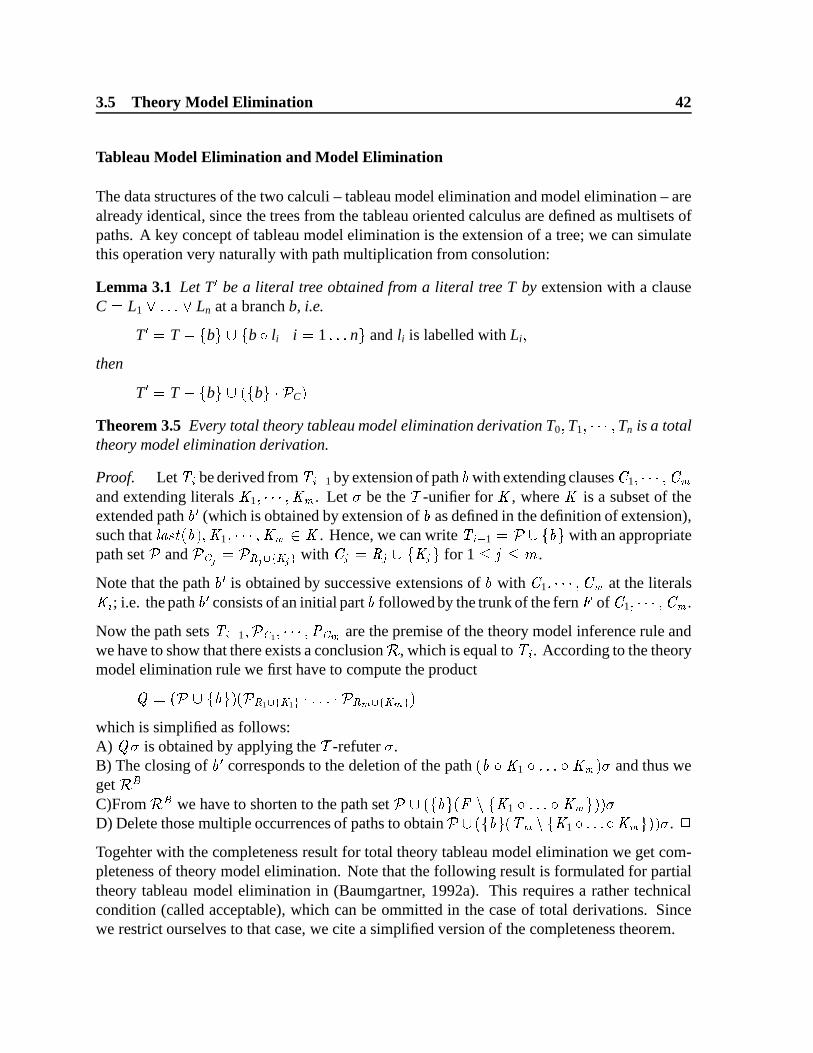
3.5 Theory Model Elimination 42
Tableau Model Elimination and Model Elimination
The data structures of the two calculi – tableau model elimination and model elimination – arealready identical, since the trees from the tableau oriented calculus are defined as multisets ofpaths. A key concept of tableau model elimination is the extension of a tree; we can simulatethis operation very naturally with path multiplication from consolution:
Lemma 3.1 Let T � be a literal tree obtained from a literal tree T by extension with a clauseC � L1
� � Ln at a branch b, i.e.
T � � T� � b � � � b � li � i � 1 n � and li is labelled with Li
�then
T � � T� � b � � � b � �
C�
Theorem 3.5 Every total theory tableau model elimination derivation T0� T1
� � Tn is a totaltheory model elimination derivation.
Proof. Let � �be derived from � � � 1 by extension of path with extending clauses � 1
� � � �and extending literals � 1
� � � � . Let � be the�
-unifier for � , where � is a subset of theextended path � (which is obtained by extension of as defined in the definition of extension),such that
� � � � � � � 1� � � � � � . Hence, we can write � � � 1 � � � � � with an appropriate
path set�
and� � � � � �
�� � �
� with � � � � � � � � � � for 1 � � � � .
Note that the path � is obtained by successive extensions of with � 1� � � � at the literals
� �; i.e. the path � consists of an initial part followed by the trunk of the fern
�of � 1
� � � � .
Now the path sets � � � 1� �
1� � � �
are the premise of the theory model inference rule andwe have to show that there exists a conclusion , which is equal to � �
. According to the theorymodel elimination rule we first have to compute the product
� � � � � � � � �1 �
� �1 � � � �
�� � �
� �which is simplified as follows:A) � � is obtained by applying the
�-refuter � .
B) The closing of � corresponds to the deletion of the path � � 1 � � � � � � and thus weget �C)From � we have to shorten to the path set
� � � � � � � � 1 � � � � � � � �D) Delete those multiple occurrences of paths to obtain
� � � � � � � � � 1 � � � � � � � � . �Togehter with the completeness result for total theory tableau model elimination we get com-pleteness of theory model elimination. Note that the following result is formulated for partialtheory tableau model elimination in (Baumgartner, 1992a). This requires a rather technicalcondition (called acceptable), which can be ommitted in the case of total derivations. Sincewe restrict ourselves to that case, we cite a simplified version of the completeness theorem.

3.6 Theory connection method 43
Theorem 3.6 ((Baumgartner, 1992a)) Let�
be a theory and M be a�
-unsatisfiable clauseset. Let C � M be such that C is contained in some minimal
�-unsatisfiable subset of M. Then
there exists a total theory tableau model elimination refutation of M with top clause C.
Theorem 3.7 (Completeness of total theory model elimination) Let�
be a theory and Mbe a
�-unsatisfiable clause set. Then there exists a total theory model elimination refutation
of M.
Proof. From the completeness of theory tableau model elimination (theorem 3.6) we know,that there exists a theory tableau model elimination derivation of the empty clause and fromtheorem 3.5 we conclude that there is a theory model elimination refutation as well. �
3.6 Theory connection method
In the present section we discuss a theory version of the connection method according to W.Bibel. According to the conventions of this paper we will consider only formulas in clauseform. The connection method is not restricted to that class of formulas. We will presentthe classical version of the connection method following (Bibel, 1987)5. However, we willtranscribe this version into a refutational form. This way we allow the reader to concentrateon the essential differences and similarities of the connection method in comparision with theother calculi discussed in this paper.
3.6.1 Informal explanation
Let us introduce some notions which are usually used in the context of the connection method.
Let us recall from 3.1.1 that a set of clauses is called a matrix. The following notion generalizesthe notion of a connection from subsubsection 3.1.2. A
�-connection in a matrix � is a set
of literals which contains from each clause from � at most one literal and which can be made�-complementary by instantiation. If the set of the elements of a path � through a matrix
contains a set � of literals then � is said to span � . Let � be a set of sets of literals. Then �spans the matrix � if for every path � through � there is a � � � that spans � . Now we canformulate the idea of the connection method.
In order to refute a clause set � the connection method tries to find a set � of instancesof clauses from � such that there is some set of
�-complementary sets of literals which
is spanning � . Under the name connection method there exists a variety of algorithms forconstructing systematically such an instance � . The approaches differ mainly in the datastructure which is used to represent the set of paths
�which should be checked for the
existence of a spanning�
-complementary set. In the version presented here�
is the fern of
5For a more recent introductory presentation see (Bibel, 1992).

3.6 Theory connection method 44
� 1� � � with trunk
�1 � � � where for every � � 1 � � � � �
is a subclause of a clausefrom � and for � � � � 1 � � � � � � � � �
and � � must not be subclauses of the sameclause in � . Then
�1 � � � � 1 is called the actual path and
� the actual goal. This notionreflects that the procedure tries as the next step to span the trunk or its extension.
Now let us consider a the following clause set � and let us track some steps of a derivationbased on the connection method with the built-in theory
�from our running example:
�:
(T-1) � � ��� �
� � � � � � � � � � � � � � � � � � � � � � � � �(T-3) � � �
� � � � � � � � � � � � � �
�:
(1) � � � � � � � � � � � � �
� � � �(2)
� � � � � � � � � � � �
(3) ��� �
� � � � � �� � � �
The clause set � which is actually under consideration is represented as a matrix where eachrow represents the elements of a clause. We start the derivation with the fern of one clause,namely clause (1), with trunk � � � � � �
� � � � � . The elements of the actual path will be in adashed box. The actual goal will be pointed by a small arrow. The elements of each of theclauses which form the fern are placed on the right of the corresponding elements of the trunk.Thus, the initial matrix looks as follows.
� � � � � � � � � � � �
� � � ��
(4)
In our example we can try an extension step by entering new clause copies to the initialclause set at the bottom of the matrix and applying a substitution to the extended matrix. Thisextension must yield a
�-refutable extension of the actual path via the actual goal. The actual
goal and the literals� � � � � � �
� � � � � and ��� �
� � � � from clauses (2) and (3) (respectively)form a
�-connection. A
�-refuter for that set is � 1 � � � �
� � � � � . So entering copiesof clauses (2) and (3), applying � to the matrix, marking the
�-complementary path with a
connection (the triple arc) and putting the elements of the new actual path into dashed boxes

3.6 Theory connection method 45
yields the following matrix.
� � � � � � � � � � �
��� �
� � � � � � �
� � � � � � � � � � � �
�� � � �
�� � � ��
(5)
It remains to span the paths in the fern determined by the new actual path. As next step wetry a second inference rule, reduction that allows inferencing without adding new clauses tothe matrix. Consider � � � � � �
� � � � � from the first row and �� � � � from the third row. By
theory clause � �3 � they are
�-refutable with
�-refuter � 2 � � � �
� � � � � . So � 2 canbe applied to the matrix and the
�-connection can be established as shown below. Now we
have spanned all paths starting from � � � � � � � � � � � . Thus, it remains to span paths starting
from �� � � � . The actual path now is empty and the actual goal is �
� � � � . We arrive atthe following matrix.
� � � � � � � � � � �
��� �
� � � � � � �
� � � � � � � � � � � �
�� � � �
�� � � �
�
(6)
Here we leave our sample derivation. We only mention that the derivation will be completedif the fern will have length zero. Then every path through the matrix is spanned by a
�
-complementary set of literals.
3.6.2 Formal definition
The extension and the reduction step of the theory connection calculus may be expressed byone single instantiation of the consolution rule.
Definition 3.21 (Total theory connection method) Let�
be a theory and�
a set of clauses.The inference rule total theory inference is defined as follows:

3.6 Theory connection method 46
�1 � � p1
��R2 �
�L2 �
...�Rn �
�Ln �
where
1.�
1 � � p1� is a fern of C1
� � Cm with trunc p1 where for j � 1 � � m Cj is a subclauseof an instance of a clause from C.
2. � Li� � Ri are pairwise variable disjoint copies of clauses from C (for i � 2 n).
3. for some subset q of the literal set of p1 the set � q � L2� � Ln
� is minimal�
-refutable.Let
�be a CSR for that set.
4. The simplification of the product� � � 1 � � p1� � � R2 �
�L2 � � � Rn �
�Ln � �
is done in the following way:
A)� � is obtained from
�by finding of a
�-refuter � � �
for � q � L2� � Ln
�(which exists by 3.)
B) All paths q� � � � satisfying the conditions
tail p1� � q� � length q� � � length p1
� � n and � q � L2� � Ln
� � q� �will be deleted. Call the resulting set B.
C) If F is the fern of � L2� � R2
� � � Ln� � Rn with trunk L2 � � Ln then obtain C
from B by shortening to the path set that is specified as follows:
� B � � � 1 � � � p1� F � � L2 � � Ln
� � � � � �In step B) some paths p may have been deleted such that K � last p � satisfiesK � Cn and K
�� Ln. Those paths belong to�
1 � � � p1� F � � L2 � � Ln
� � �
Therefore we have to cut with B.
D) Let � C.
A total theory connection derivation is defined as a linear theory consolution derivation whereevery theory consolution inference is a “total theory connection inference”. �

3.6 Theory connection method 47
Example. In order to illustrate the previous definition let us consider again the theory andclause set as used above in the informal presentation. We discussed in detail the first inferencestep, an extension, in order to illustrate the model elimination case. Now for illustrating theformalization of the theory connection method we will redo the second inference step of oursample run which is a reduction. After the first step we arrive at the following path set6:�
2 � � � 2� � � � � � � � �
� � � � � � � � � � � � � � � � � � � �
� � � � � �� � � � �
Here we choose � 2 � � � � � � � � � � � � � � � � � � � �
� � � � � � �� � � � . The path set
�2 � � � 2
� willbe processed in the following inference step:
� � � � � � � � � � � � � � � � � � � �
� � � � � � �� � � � � �
� � � � �� �
� � � � � � �
The resulting path set encodes the same path set as in the example of the above informalpresentation. Let us have a detailled view how this result can be achieved: Since our productconsists of one factor we have
� � �2 � � � 2
� .�
is simplified as follows: The instance ofthe consolution rule has the form�
2 � � � 2�
where
1. � 2 denotes the path which is underlined in � � . It has a maximal length in�
2 � � � 2� .
2. � � 0.
3. The subset � is � � � � � � � � � � � � � �
� � � � � .
4. A) The above underlined path
� � � � � � � � � � � � � � � � � � �
� � � � � � �� � � � � �
is selected for finding a�
-refuter � � � � �� � � � � for the
�-connection
� � � � � � � � � � � � � �
� � � � � .
B) � is obtained from� � by deletion of � �
� � � �� � � � �
C) Shortening is neither possible nor necessary.
� �D) Finally we have � �
.
6This path set is the fern of � � � � � � � � �� � � � � � � �
� � � � � �, � � � � � � � � �
� � � � � �, � �
� � � � � �with trunk� � � � � � � �
� � � � � � � � � � � � � �� � � � � �
�� � � � �

3.6 Theory connection method 48
It is astonishing how closely related the theory model elimination and theory connection methodare.
� Model elimination has a free selection function and thus allows the next subgoal to bechosen in a don’t care nondeterministically manner. In the presented version of theconnection method a trunk, i.e. a branch of maximal length, is selected for extension.This restriction makes sure that the set of unexamined paths obtained after the extensionmay be represented as a fern too (cf. proposition 1). In (Neugebauer and Schaub, 1991)there has been proposed another representation of that set by a set of hooks instead ofa fern. A hook represents the fern of � �
1� � � �
2� � � � � � 1
� � � � � � � with trunk�1 � �
2 � � � � 1 � � . This representation allows the same flexibility like the treerepresentation which is used in the tableaux model elimination.
� In step A) of simplification the role of the last literal of the path to be extended isdifferent: in the tree-notation of model elimination, the last literal corresponds to theleaf of the branch, and that literal must be “essential” in the
�-complementary literal
set (i.e. without it, the set is no longer�
-complementary). In the presented versionof the connection method, the last literal has no special meaning. Thus the modelelimination extension rule is more restrictive than the connection method inference rule.In (Petermann, 1993b) has been proved that also the extension rule of the the connectionmethod may be restricted in that way without lost of completeness. Thus, the branchingrate in the search space might be restricted like in the model elimination.
� In step B) the connection method is more effective than model elimination, since all pathswhich reach the actual clause and which become
�-complementary by the
�-refuter
are deleted. In model elimination only one path is deleted.
There are many refinements of the connection method which cut the search space essentially.For an overview see (Bibel, 1987) and (Letz et al., 1992)
Now let us formulate some results about the total theory connection method. First of all weneed a representation lemma 3.2 concerning ferns and two lemmata 3.3 and 3.4 concerningtheir structure properties. The three lemmata may be proved by simple verification. Thosefacts enable us to prove that a set of paths obtained by a total theory connection inferencefrom a fern � is again a fern. This gives a formal justification of our definition of the totalconnection inference rule.
Lemma 3.2 Let F be the fern of � C1� � � � Cn
� with trunk L1 � � Ln. Then for eachi � 1 � � n holds
Ci � � Li� � � last p � � p � F � length p � � i �
Lemma 3.3 Every subset of a fern is a fern.

3.6 Theory connection method 49
Lemma 3.4 Let � be a fern of � C1� � � � Cn
� with trunk p � L1 � � Ln and let � be a fernof � Cn
�1� � � � Cn
�m
� with trunk Ln�
1 � � Ln�
m. Then
� � � p � � � � p � � �is the fern of � C1
� � � � Cn� � � Cn
�1� � � � Cn
�m
� with trunk L1 � � Ln � Ln�
1 � � Ln�
m.
Proposition 1 Let �1 � � p1
��R2 �
�L2 �
...�Rn �
�Ln �
be a total theory connection inference. Then R is a fern.
Proof. Let � 1 � � 1 � � � � where � � 0 is allowed. Then (cf. definition 3.21)�
1 � � � 1� is
a fern of some clauses � 1� � � � with trunk � 1. Let
�be the fern of � �
2� � � 2
� � � � � � � with trunk
�2 � � � . Then according to lemma 3.4�
1 � � � � 1� � �
is the fern of� 1
� � � � � � �2� � � 2
� � � � � � � with trunk � 1 � �
2 � � � . According to lemma 3.3 R is a fern because it is a subset of thatfern. �Finally we give proof outlines of the soundness and completeness theorem for the total connec-tion method.
Theorem 3.8 Soundness Let�
be a theory and let�
be a clause set. If there exist a copy of aclause of
�, an element L � �
and a total theory connection derivation which starts from thefern of
�with trunk L then
�is
�-unsatisfiable.
Proof. Let�
be a theory and let�
be a clause set. Let�
1� � � � be a total theory connection
derivation and let � �denote the set of copies of clauses from � which have been used as
extension clauses up to the � �1 � -th inference for each � � 1 � � � . Moreover let � �
denotethe set of
�-connections which have been found up to the � �
1 � -th inference for each� � 1 � � � . Claim: � �
spans all paths � through � �such that there is no path � � � �
with� � � or � � � . In order to prove this claim it is sufficient to observe that�
1 contains all pathsthrough � 1 and that in each simplifaction step
within substeps A and B only those paths are deleted that are spanned by the considered�-connection,
within substeps C path are only shortened and
3.6 Theory connection method 50
within substep D the set of paths remains unchanged.
Clearly, if � � � � then � � spans � � . �Theorem 3.9 Completeness Let
�be a theory such that
1. the set of�
-connections is decidable,
2. for each�
-refutable literal set u a complete set of�
-refuters is enumerable.
If�
is a�
-unsatisfiable clause set then there exist a copy of a clause of�
, an element L � �
and a total theory connection derivation which starts from the fern of�
with trunk L.
Proof. Let�
be a theory and let�
be a�
-unsatisfiable clause set. >From the Herbrandtheorem proved in (Petermann, 1991b) follows that there is a set of instances � of clausesof
�and a set of
�-complementary literal sets which is spanning � . There is a ground
total connection derivation of � . This may be shown using properties of minimal spanningmatings of ferns (cf. (Petermann, 1993b)). The decidability of the set of
�-connections and
the enumerability of the CSR for each � allow to lift this ground derivation to a total connectionderivation where each inference is effective. �
Discussion:
The decidability of the set of�
-connections is necessary for the decidability of the derivationrelation. Sometimes it is not necessary to know all
�-connections and to be able to enumerate�
-refuters for all of them. For example there is a fragment of first-order logic with equalitywhich is the image of the translation of multi-modal logics following (Debart et al., 1990).Different modal systems may be described by equational theories. Fortunately, after translationthere occurs no equality sign in the formulas. This sinplifies considerably the the set of theoryconnections to be considered. In order to describe this phenomenon in (Petermann, 1993b) hasbeen studied the notion of a complete set of theory connections.
The decidability whether � � � � � � � � means in an implementation that whenever theexistence of a
�-refuter for a
�-connection is considered that in case of the non-existence
there will be a defined answer and not a failure.
The restriction that the actual goal is element of the actually found connection can be provedby careful examination of minimal spanning sets of connection.
The partial variant of theory connection method can be defined in much the same way as totaltheory resolution is modified to partial theory resolution. This is omitted here. The interestedreader is referred to (Petermann, 1993a). Paramodulation, relaxed paramodulation and RUE-resolution have been view as instances of a partial theory connection calculus. It is worth
4 Equality 51
mentioning that the residue may have more than one literal if not only the paramodulation isconsidered.
4 Equality
Being of such a fundamental importance in mathematics and nearly every area where deductionapplies, the equality relation deserves special treatment. Thus it is not surprising that in theearly days of theorem proving the equality relation was already built in. Viewed syntactically“equations” are simply literals, built from the predicate symbol “� ” and written infix. Se-mantically, the interpretation of “� ” is comitted to an equivalence relation that is closed underequality replacement for all function and predicate symbols of the language (i.e. a congruencerelation). From the viewpoint of theory reasoning, we have to deal with the theory of equality� , which can be axiomatized by the following scheme:
� : � � : � � � (Reflexivity)� � � � : � � � � � � � (Symmetry)� � � � � � : � � � � � � � � � � � (Transitivity)� � 1
� � � � � : � � � � �� � 1
� � � � � 1� � � � � � �
1� � � � ��
� 1� � � � � 1
� � � � � �1
� � � � for all � -ary function symbols�
and all 1 � � � � (
�-
Substitutivity)� � 1
� � � � � : � � � � �� � 1
� � � � � 1� � � � � � �
1� � � � � �
� � 1� � � � � 1
� � � � � �1
� � � � � for all � -ary predicate symbols� and all 1 � � � � (� -Substitutivity)
If we assume that we have only a finite number of predicate and function symbols (as is usuallythe case) then this theory of equality is finite too. Thus also “equality” could be dealt with inthe trivial way: simply add the clause form of these axioms to a given specification and relyon the no-theory calculus. This however is prohibited for well-known efficiency reasons. Thetheory of equality should be handled at least as carefully as any other theory following thediscussion of the previous chapters e.g. 3.
4.1 Dealing with Equality via Total Theory Reasoning
Here we discuss the possibility of building in the theory of equality by total theory reasoningfollowing our discussion in section 2.1.

4.1 Dealing with Equality via Total Theory Reasoning 52
For a given literal set we have to accomplish an � -refuter. For this purpose it might be usefulto know of the syntactical form of � -complementary literal sets. It is as follows (Petermann,1991b):
� � � where�
is a set of equations and � consists either of two literals � �1
� � � �and � � 1
� � � � or of one negated equation � � � with � � 0 such that
�� � � � ��� �
0
� � � � �
Both cases have an obvious intuitive meaning. The sides of each term pair � � � � � � � mightbecome equal by subsequent substitutions of subterms which occur as one side of the equationsin
�by the other side of such an equation. Obviously this raises a contradiction. Due to this
syntactic structure the dedicated reasoner has to solve the following problem:
Given a set�
of equations and some pairs of terms � � � � � � � . Is there a substitution� such that for all equations � � � � � � � holds that
� � � � � � � � � � � � is � -complementary?
It can be shown (Baumgartner, 1992b) that this problem is equivalent to the so-called rigid� -unification problem (Gallier and Snyder, 1990). It is formulated as follows:
Given a set�
of equations and some pairs � � � � � � � . Is there a substitution �such that all equations � � � � � � � are a logical � -consequence of
� � , where allvariables are treated as constants?
Let us consider the following clause specification in the spirit of the introductory example:
(4) �� � � � � �
�� � � � � � � � � � � � � � � � � � �
(5) � � � � � � � � � � � � � � � � � �
(6) �� � �
� � � � �
A useful query is for example to ask for the father of sue. An answer might be found by addingthe clause
�� � � � � � � � � � � and refuting the thus obtained clause set � . This example will
be processed by the various approaches below. Of course there is a trivial solution, namely� � �
�� � � � � � � � � � which simply says that the father of Sue is the father of Sue. We will
suppose the deductions below to be controlled in such a way that the more interesting answer� � �
� � � � � results. Refutations which return that answer rely on the fact that there are twoliteral sets
��
� � � � � � � � � � � � � � � � � � � � � � � � � � � � � � � � � � � � � � �
�� � � � � � � � � � � �
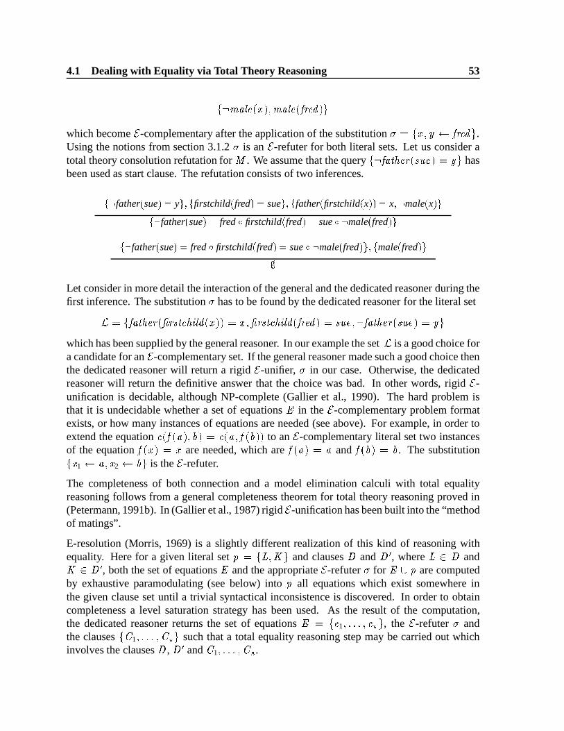
4.1 Dealing with Equality via Total Theory Reasoning 53
� �� � � � � � �
� � � � � � � � �
which become � -complementary after the application of the substitution � � � � � � �� � � � � .
Using the notions from section 3.1.2 � is an � -refuter for both literal sets. Let us consider atotal theory consolution refutation for � . We assume that the query �
�� � � � � � � � � � � � has
been used as start clause. The refutation consists of two inferences.
� father � sue � � y� �firstchild � fred � � sue� �
father � firstchild � x � � � x male � x � �� father � sue � � fred � firstchild � fred � � sue � male � fred � �
� father � sue � � fred � firstchild � fred � � sue � male � fred � � �male � fred � �
�
Let consider in more detail the interaction of the general and the dedicated reasoner during thefirst inference. The substitution � has to be found by the dedicated reasoner for the literal set
� � ��
� � � � � � � � � � � � � � � � � � � � � � � � � � � � � � � � � � � � � � �
�� � � � � � � � � � � �
which has been supplied by the general reasoner. In our example the set�
is a good choice fora candidate for an � -complementary set. If the general reasoner made such a good choice thenthe dedicated reasoner will return a rigid � -unifier, � in our case. Otherwise, the dedicatedreasoner will return the definitive answer that the choice was bad. In other words, rigid � -unification is decidable, although NP-complete (Gallier et al., 1990). The hard problem isthat it is undecidable whether a set of equations
�in the � -complementary problem format
exists, or how many instances of equations are needed (see above). For example, in order toextend the equation �
� � � � � � � � �
� � � to an � -complementary literal set two instances
of the equation
� � � � � are needed, which are
� � � � �
and
� � � . The substitution
� � 1� � � � 2
� � is the � -refuter.
The completeness of both connection and a model elimination calculi with total equalityreasoning follows from a general completeness theorem for total theory reasoning proved in(Petermann, 1991b). In (Gallier et al., 1987) rigid � -unification has been built into the “methodof matings”.
E-resolution (Morris, 1969) is a slightly different realization of this kind of reasoning withequality. Here for a given literal set � � � � � � � and clauses � and � � , where
� � � and� � � � , both the set of equations
�and the appropriate � -refuter � for
� � � are computedby exhaustive paramodulating (see below) into � all equations which exist somewhere inthe given clause set until a trivial syntactical inconsistence is discovered. In order to obtaincompleteness a level saturation strategy has been used. As the result of the computation,the dedicated reasoner returns the set of equations
� � � �1� � � � , the � -refuter � and
the clauses � � 1� � � � such that a total equality reasoning step may be carried out which
involves the clauses � , � � and � 1� � � .
4.2 Dealing with Equality via Partial Theory Reasoning 54
4.2 Dealing with Equality via Partial Theory Reasoning
In the previous approach we had to guess in one step an � -complementary literal set and tocompute an � -refuter. Now we break this huge step into smaller ones. Two main ways to doso have been studied.
Paramodulation-like setting: We apply equations by substituting “equals by equals” in orderto transform terms which are suspected to be equal. We are allowed to use unification inorder to make an equation applicable. This is rather a bottom-up approach.
RUE-resolution-like setting: We consider the “difference” between corresponding terms, inorder to determine some equations which are sufficient for their equality. This is rathera top-down approach.
In both cases the considered rules are thought to produce either complementary pairs or negatedequations. Both cases will be viewed now as instances of partial theory reasoning.
4.2.1 Paramodulation-like Calculi
Let us recall from section 4.1 that if an � -refuter � has been found for literal set� � � then
corresponding term pairs in � � may be made equal by substituting “equals by equals” usingequations from
� � . In a paramodulation-like setting, the set� � � and the � -refuter will be
approximated by number of single replacements of “equals by equals”. To be equal meansnow “equal up to some substitution”.
Let us examine the co-operation between general and dedicated reasoner in this situation. Thegeneral reasoner now has to supply literal sets
� � � � � � � � �� � �
where� � denotes a subterm occurrence in
�and
� �� � is a nondeterministic notation for eitherthe literal
� � � or the literal � � �.
�may contain the equality predicate. The dedicated
reasoner has to return a pair � � � � � � � � � �
if a most general unifier � of� � and
�exists.
� � � � � � � means that one occurrence of� � in
�is
replaced by � . Obviously, the literal set
� � � � � � � � � � �� � � � � � � � � � � �
is � -complementary. Thus, the pair
� � � � � � � � � �

4.2 Dealing with Equality via Partial Theory Reasoning 55
is a residue for the literal set� � � � � � � � �
� � � A partial � -reasoning step using this way of forming the residue will be called a paramodulationinference.
� � is called the term paramodulated into.
Although well-known we prefer to give a short example of paramodulation in order to easecomparison with other approaches below. We return to our example from 4.1. We could com-pute the
�� � � � � of
� � �by splitting the first total theory consolution step into one paramodulation
and one extension step. This fragment of the derivation has the following form:
� � � � � � � � � � � � � � � � � � � � � �
�� � � � � � � � � � � � � � � � � � � � �
� � � � � �� � 1
� � 2�
� � 1� � 2
� � � �
� � � � � � � � � � � �� � � � � � � � � �
� � � � � � � � � � �� � �
� � � � � �where
� 1 � � � � � � � � � � � � � � � � � � �
��
� � � � � � � � � � � � � � � � � � � � �
� � � � ��
� � � � � � � � � �
� � � �
� 2 � � � � � � � � � � � � � � � � � � � � �
� � � � � � � �
The more interesting first step in that derivation is a paramodulation into the term � � � � � � � � � � � .The pair
� � ��
� � � � � � � � � �
� � � � � with � � � � � �� � � � �
is a residue for the set of literals
� � � � � � � � � � � � � � � � � � � �
�� � � � � � � � � � � � � � � � � � � �
The path � 1 has been obtained by adjoining the path from the residue to the path
� � � � � � � � � � � � � � � � � � �
�� � � � � � � � � � � � � �
� � � � � � �
� � � �
Obviously, the paramodulation inference is much simpler than the the computation of an � -refuter. But this simplification must be paid for by a large search space introduced by thechaining of paramodulation steps. In the present version paramodulation cannot use any hintwhich equation should be applied for paramodulation in order to enable further reasoning stepsto be made. Thus, the enormous search space will be entered without any guidance. Therefore,improvements are urgently needed (see below).
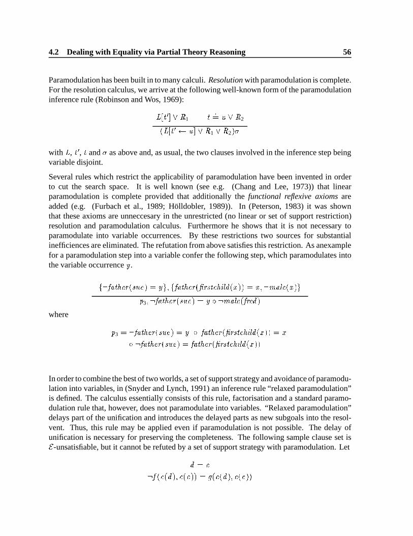
4.2 Dealing with Equality via Partial Theory Reasoning 56
Paramodulation has been built in to many calculi. Resolution with paramodulation is complete.For the resolution calculus, we arrive at the following well-known form of the paramodulationinference rule (Robinson and Wos, 1969):
� � � � � � � 1� �� � � � 2
� � � � � � � � � 1� � 2
� �
with�
,� � , �
and � as above and, as usual, the two clauses involved in the inference step beingvariable disjoint.
Several rules which restrict the applicability of paramodulation have been invented in orderto cut the search space. It is well known (see e.g. (Chang and Lee, 1973)) that linearparamodulation is complete provided that additionally the functional reflexive axioms areadded (e.g. (Furbach et al., 1989; Holldobler, 1989)). In (Peterson, 1983) it was shownthat these axioms are unneccesary in the unrestricted (no linear or set of support restriction)resolution and paramodulation calculus. Furthermore he shows that it is not necessary toparamodulate into variable occurrences. By these restrictions two sources for substantialinefficiences are eliminated. The refutation from above satisfies this restriction. As anexamplefor a paramodulation step into a variable confer the following step, which paramodulates intothe variable occurrence � .
� �
� � � � � � � � � � � � � ��
� � � � � � � � � � � � � � � � � � � � �� � � � � �
� 3�
�� � � � � � � � � � � � �
� � � � � � � �
where
� 3 � �
� � � � � � � � � � � ��
� � � � � � � � � � � � � � � � � � ��
�� � � � � � � � � �
�� � � � � � � � � � � � � � � � �
In order to combine the best of two worlds, a set of support strategy and avoidance of paramodu-lation into variables, in (Snyder and Lynch, 1991) an inference rule “relaxed paramodulation”is defined. The calculus essentially consists of this rule, factorisation and a standard paramo-dulation rule that, however, does not paramodulate into variables. “Relaxed paramodulation”delays part of the unification and introduces the delayed parts as new subgoals into the resol-vent. Thus, this rule may be applied even if paramodulation is not possible. The delay ofunification is necessary for preserving the completeness. The following sample clause set is� -unsatisfiable, but it cannot be refuted by a set of support strategy with paramodulation. Let
� � �
� � � � � � � � � � � � � � � � � � �

4.2 Dealing with Equality via Partial Theory Reasoning 57
�
� � � � � � � � � � � � � � � � � �� � � � � � � � � � � �
� � � � � � � � � � �
be a set of equations with set of support ��
� � � � � � � � � � ��
� � � � � � � � � � � . Thereason for paramodulation (without substituting into variables) to fail is that there is no wayto paramodulate from
� � � � � into
� � � � � � � � � nor from � � � � � into � � � � � � � � � nor
from� � � � � into
� � � � � � � � � . However, relaxed paramodulation from, say,
� � � � � �� � � � � into
� � � � � � � � � is possible. This inference returns � � � � � � � � � � �� � � � � � � � � � � � � � � � � � � � as a kind of a residue. All of these additional goals may be
solved by use of the equation� � �
. This technique is much in the spirit of RUE-resolution(Digricoli and Harrison, 1986) with the important restriction that the delayed subgoals (thecorresponding concept in RUE-resolution is “disagreement set”) can be restricted to variable-term pairs. Unfortunately the completeness of “relaxed paramodulation” with set of supportstrategy has not been proved yet.
As a concluding improvement of paramodulation we will briefly sketch basic paramodulation(Bachmair et al., 1992). The term “basic” was coined in (Hullot, 1980) in the context ofnarrowing (section 2.2) and means the same thing for paramodulation: in basic paramodulation,it is forbidden to paramodulate into occurrences introduced by previous inference steps. Statedpositively, paramodulation is allowed only into such occurrences that are already present in theinput set. For example, suppose that the clause � � � � � � � is resolved with � �
� � � � �
yielding � � �
� � � � . Then � � �
� � � � can be paramodulated with, say,
� � � � �
to � � � � � ;however, this is no basic paramodulation step, since � � � does not contain the
�-term to be
paramodulated upon. Thus, basic paramodulation is a serious restriction of the applicabibiltyof paramodulation. Moreover, in basic paramodulation it is not necessary to paramodulate intovariables; also it is compatible with ordering restrictions (section 4.2.3).
A paramodulation-like treatment of equality was carried out for the tableau method (Fitting,1990) in (Jeffrey, 1967) and (Poppelstone, 1967), for model elimination (Loveland, 1978),for the connection method (Petermann, 1991a) and for connection graphs (Siekmann andWrightson, 1980). Paramodulation with order-sorted theories has been considered in (Walther,1983).
In the next parts of the paper we discuss in more detail two further alternatives for restrictionsof the paramodulation rule which have been considered in the literature:
1. Make the application of equations more goal-oriented: choose first candidates for acomplementary pair and look which equations should be used. Solve these equations byparamodulation.
2. Restrict the applicability of the paramodulation rule by order restrictions. For instancemake sure that clauses are not growing w.r.t. a term ordering.
4.2 Dealing with Equality via Partial Theory Reasoning 58
4.2.2 RUE-Resolution-like
Let us discuss in more detail one strategy of making paramodulation more efficient. Theimprovement is given by the following advice.
� Try to unify corresponding term pairs first.� Paramodulate only into those terms which cannot be made equal this way.
Applying this strategy to the previous example the prover might “think”: Let’s try to make an� -complementary literal set from
�� � � � � � � � � � � and
�� � � � � � � � � � � � � � � � � � � .
Then the equation � � � � � � � � � � � � � � �would be needed to achieve that goal. The hint, that� � � � � � � � � � � � � � �
should be solved as a subgoal follows from the failure of the unificationalgorithm7. Since on the outermost level the
�� � � � � -function symbols are the same in both
terms, it suffices to prove that the argument terms of the left hand side, and the right hand sideare equal. In other words, the left hand side has to be “decomposed”8 into the new subgoal � � � � � � � � � � � � � � �
. The right hand sides immediately unify by, say, � � � � � . This exampledemonstrates the main idea of RUE-resolution: unify the terms “as much as possible”, andprove equality of non-unifying terms later. In RUE-terminology the most general substitutioninvolved in this is called a most general partial unifier and the non-unifying part is called thedisagreement set. For a given unification problem several disagreement sets may exist. Let usexamine an example related to that in subsection 4.1. In our terminology the example situationcan be formulated as the path
�
� � � � � � � � � � � ��
� � � � � � � � � � � � � � � � � � � � � � � � � � � � � � � � � � �
which becomes � -complementary with the substitution � � � � � � � � . Thus, the pair
� � � � � � � � � � � � � � � � � � �forms a residue for the literal set
� �
� � � � � � � � � � � ��
� � � � � � � � � � � � � � � � � � � � The new goal � � � � � � � � � � � � � � �
may be solved together with the fact � � � � � � � � � � � � � � �� � �
. The corresponding two step consolution refutation fragment looks as follows. The firststep is adding a residue, the second step is an extension. Let
� 1 � �
� � � � � � � � � � ��
�� � � � � � � � � � � � � � � � � � � � � � � � � � � � � � � � � � �
� 2 � �
� � � � � � � � � � � � �� � � � �
7Suppose the unification is according to the transformational approach to unification (J.-P. Jouannaud, 1991).Then the failure already occurs after one application of the decomposition rule.
8A unification algorithm based on an transformational approach which also includes a decomposition rule canbe found in (J.-P. Jouannaud, 1991)
4.2 Dealing with Equality via Partial Theory Reasoning 59
� �
� � � � � � � � � � � � � ��
� � � � � � � � � � � � � � � � � � � � �� � � � � �
� � 1� � 2
�� � 1
� � 2� � � � � � � � � � � �
� � � � � � � � � ��
�� � � � � � � � � �
� � � � � �� � �
� � � � � �Let us compare the present tactic with the paramodulation rule. The underlying � -complementaryliteral set has a similar structure:
� � � � � � � � � �� � � � � � � � � � � � � �But now we construct the pair
� � � � �� � �as the residue for the literal set
� � � � � � � � � � � � � � � �
The construction of the residue is now more goal-oriented. We have another restriction of thegeneral rule for computing the residue.
It should be noted that in general it is not possible for completeness reasons to restrict to the“most specific” disagreement set. This is the disagreement set that results from unification“as much as possible”. An example below will show this. This claim may illustrated by thefollowing example (Anderson, 1970).
(1) � �
� � � � � � � � � � � � � � � � �(2) �
� � � � � � �
(3) � � � � � � �(4)
� � � �
� � �
(5)� � � � � �
A prover which is allowed to paramodulate only on unification failure comes up with a unifiercontaining
either � � � � � (if � �
� � � � � � � from the first and � �
� � � � � � from the secondclause are considered)
or � � � � (if � � � � � � � � � from the first and � � � � � � � from the third clauseare considered).
But the unique useful substitution � � � � � may be found only in a more flexible way. Oneimprovement is the so called RUE-resolution due to Digricoli (Digricoli and Harrison, 1986).

4.2 Dealing with Equality via Partial Theory Reasoning 60
There the prover is allowed to look ahead for paramodulation possibilities before going deeperapplying the decomposition rule. In our example the prover is allowed to transform theunification problem �
� � � �
� � � � (called disagreement set in (Digricoli and Harrison, 1986))
into ��
� � ��
� � � using the fourth clause. This way the substitution � � � � � may be detectedin fact. Nevertheless the inference rules are rather complicated and it is not known to theauthors whether the overhead is not too much.
Another improvement is based on a level saturation strategy as given and proved to be completein (Anderson, 1970). The connection graph calculus was extended with an equality handling inthe spirit of RUE-resolution by means of equality graphs (EGC-procedure) in (Blasius, 1987).A matrix calculus with a RUE-resolution-like inference rule has been proved to be completein (Petermann, 1991c). A treatment of equality which is similar to the RUE-resolution wascarried out for the tableau method (Fitting, 1990) in (Reeves, 1987).
4.2.3 Ordering Strategies
Except rigid � -unification, for which experimental results are not yet available, all the methodsdescribed so far for equality handling could not prove to be sufficient for really hard practicalproblems. (Ohlbach and Siekmann, 1991) report various discouraging results with paramo-dulation and the EGC-procedure within the connection graph calculus. As a solution, recentresearch concentrates on the application of ordering restrictions. These methods can beseen as extensions of term rewriting and the Knuth-Bendix completion procedure (Knuth andBendix, 1970). A good overview over term rewriting, completion and some of its extensionscan be found in (Plaisted, 1993).
Calculi and proof procedures for full first order order-restricted equational theorem provingwere proposed in (Bachmair, 1991; Bachmair and Ganzinger, 1990a; Bachmair and Ganzinger,1990b; Zhang and Kapur, 1988; Hsiang and Rusinowitch, 1986; Hsiang and Rusinowitch, 1987;Kounalis and Rusinowitch, 1991; Rusinowitch, 1991; Kirchner et al., 1990; Socher-Ambrosius,1990). These systems are basically paramodulation-like, however the possible inferences arehighly restricted by orderings, which have to be given as an input parameter. More precisely,the given ordering � must satisfy the following properties (“complete reduction ordering”):
1. � is stable under substitution, i.e.�
��
implies� � �
� � for all� � � � � .
2. � is monotonic, i.e.�
��
implies � � � � � � � � � for all� � � � � .
3. � is ground-total.
4. � is well-founded.
The inference rules below make heavy use of such a given ordering. One main application isto direct the use of equations, i.e. to allow only one side of an equation as a paramodulatingterm. Which side of an equation
� �� � is to be used, is determined by the ordering: if �
4.2 Dealing with Equality via Partial Theory Reasoning 61
has to substitute the term�
then � should be the smaller side of� �
� � . However, in generalonly in the ground case can it be achieved that
� �� �
implies that either�
��
or�
��
(see(Dershowitz, 1987) for an overview about orderings). In order to compute with non-variableterms, the � -relation is “lifted” to the condition “
��”; this means that if in the ground case an
inference were legal if�
� � , then it is legal in the general case if� �� � . Similarly, for sets of
literals the notion of a “greatest literal” lifts to that of a “maximal literal”: a literal�
is maximalrelative to a set if for none of the literals � in that set holds
� �� . Additionally the term
ordering must be extended to equations and to literals; this can be done e.g. lexicographically.
Essentially the several order-restricted paramodulation calculi restrict the above paramodula-tion inference rule in the following way:
� � � � � � � 1� �
� � � � 2
� � � � � � � � � 1� � 2
� �if
1.� � � � � � is maximal relative to � 1 � and � �
� � � � is maximal relative to � 2 � (onlymaximal literals in clauses may be selected for the inference; also comparison is doneafter application of � , since after instantiation more information is available, possiblyruling out some inferences).
2.� � �� � � (the substitution of
� � by � � must not cause a growth of the literal) and if� � � � � �
is an equation� � � � � � �
� � � � � � �� � � then
� � � � � � �� � � (it suffices to paramodulate intobigger sides of equations). In this case, the inference is called a superposition inference.
3.� � is not a variable occurrence.
Let us compute our example with this restricted variant. We need an ordering. For the sake ofsimplicity, assume that literals are ordered �
� � � � � ��1 � �
2 for any� � �
1� �
2, and for functionsymbols we order � � � � � � � � � �
� � �, and assume e.g. a recursive path ordering based on this
ordering (see (Dershowitz, 1987) for an overview about orderings). The ordering among theother function symbols does not matter. Suppose again that we want to refute
7 � � �
�� � � � � � � � �
According to restriction 3. we cannot paramodulate into � in (7). Furthermore we cannotparamodulate into
� � �with (5), because in (5) we have � � � � � � � � �
� � � � � �� � �
and such astep would violate restriction 2. Also we cannot use (4) to paramodulate into
�� � � � � � � � � of
(7), because in (4) �� � � � � �
�� � � � � � � � � � � � � � � � � � � and hence according to restriction
1. Only �� � � � � may be used in an inference. A legal step is to resolve (4) with (6), which
yields:
8 ��
� � � � � � � � � � � � � � � � � � � � �
� � � �
5 Conclusion 62
Now (5) can be used to paramodulate into � � � � � � � � � � � � � � in (8), which yields
9 ��
� � � � � � � � � �
� � � �
Now paramodulating (9) into
�� � � � � � � � � of (7), and a final resolution with � � � completes
the proof.
It should be indicated by this example that ordering restrictions are a very effective tool fordisallowing many otherwise possible inferences. For example, the topmost step in the aboveparamodulation refutation is no legal inference in the restricted calculus, because it violates therestriction 1 and 2. As a general property these ordering restrictions seem to be only possibleat the price of giving up the linear, top-down strategy as in the unordered case. However, as animprovement in this direction in (Socher-Ambrosius, 1992) a more goal-oriented completionstrategy is proposed.
As a special case, the term ordering might be strong enough to direct all the equations intorewrite rules, which means that in inferences only the left side needs to be considered forreplacement by the right side. Sometimes the input clauses, short of the query, can be closedunder application of the above ordered inference rule and yield a finite clause set. This iseasier to achieve if additionally simplification techniques are applied (see again (Bachmair andGanzinger, 1991; Bachmair and Ganzinger, 1990b)). This finite set can be used to decide theword problem in the given equational theory. In the infinite case a semi-decision procedureresults (see also (Hsiang and Rusinowitch, 1987) for such an “unfailing” procedure). Thisshows that such calculi are closely related to the Knuth-Bendix completion procedure; indeed,that procedure can be seen as an instance of them.
We are not aware of any research going on in a non-resolution setting.
5 Conclusion
We have presented a classification of theory reasoning methods for first order predicate calculi.We have distinguished between literal, term and variable level reasoning. The main focus ofthe paper is literal level theory reasoning, which is presented for various calculi in a uniformmanner. For this we used the consolution calculus, which was defined in a partial and a totaltheory variant. This framework was then used in the main part of the paper to present theoryresolution, theory model elimination and a theory connection method. For the total variants ofthese calculi we have proven completeness.
The advantages of such a uniform view of various calculi are both the possibility of using thesame formal machinery for different calculi, and the ability to investigate differences in detail.
Since efficient equality handling is one of the central issues in theorem proving we have

REFERENCES 63
discussed this in a special section. Again, we presented methods like paramodulation and RUE-resolution as special cases of partial theory reasoning in the framework of theory consolution.
References
Anderson, R. (1970). Completeness results for E-resolution. In Proceedings AFIP 70, SpringJoint Comp. Conf., AFIPS Press, Reston VA, pages 653–656.
Bachmair, L. (1991). Canonical Equational Proofs. Progress in Theoretical Computer Science.Birkhauser.
Bachmair, L. and Ganzinger, H. (1990a). Completion of First-Order Clauses with Equality byStrict Superposition. In Proc. Second Int. Workshop on Conditional and Typed RewriteSystems, LNCS. Springer.
Bachmair, L. and Ganzinger, H. (1990b). On Restrictions of Ordered Paramodulation withSimplification. In Stickel, M., editor, Proc CADE 10, LNCS 449, pages 427–441. Springer.
Bachmair, L. and Ganzinger, H. (1991). Rewrite-Based Equational Theorem Proving WithSelection and Simplification. Technical Report MPI-I-91-208, Max-Planck-Institut furInformatik.
Bachmair, L., Ganzinger, H., Lynch, C., and Snyder, W. (1992). Basic Paramodulation andSuperposition. In Kapur, D., editor, Proc. 11th CADE, pages 462–476. Springer.
Baumgartner, P. (1992a). A Model Elimination Calculus with Built-in Theories. In Ohlbach,H.-J., editor, Proceedings of the 16-th German AI-Conference (GWAI-92), pages 30–42.Springer. LNAI 671.
Baumgartner, P. (1992b). An Ordered Theory Resolution Calculus. In Voronkov, A., edi-tor, Logic Programming and Automated Reasoning (Proceedings), pages 119–130, St.Petersburg, Russia. Springer. LNAI 624.
Baumgartner, P. and Furbach, U. (1992). Consolution as a Framework for Comparing Calculi.Forschungsbericht 11/92, University of Koblenz. (to appear in Journal of SymbolicComputation).
Bibel, W. (1987). Automated Theorem Proving. Vieweg, 2nd edition.
Bibel, W. (1992). Deduktion, volume 6.2 of Handbuch der Informatik. Oldenburg.
Blasius, K. (1987). Equality Reasoning Based on Graphs. SEKI-Report SR-87-01, UniversitatKaiserslautern.

REFERENCES 64
Blasius, K. and Burckert, H.-J. (1989). Deduction Systems in Artificial Intelligence. Horwood,Chichester.
Brachmann, R., Fikes, R., and Levesque, H. (1983). KRYPTON: a functional approach toknowledge representation. IEEE Computer, 16(10):67–73.
Burckert, H. (1990a). A Resolution Principle for Clauses with Constraints. In Stickel, M. E.,editor, Proc CADE 10, pages 178–192. Springer. LNCS/LNAI 449.
Burckert, H.-J. (1990b). A Resolution Principle for Clauses with Constraints. Research ReportRR-90-02, DFKI.
Burckert, H.-J. (1992). A Resolution Principle for Clauses with Restricted Quantifiers, volume568 of LNAI. Springer.
Burckert, H.-J., Herold, A., Kapur, D., Siekmann, J., Stickel, M., Tepp, M., and Zhang, H.(1988). Opening the AC-Unification Race. Journal of Automated Reasoning, 4:465 –474.
Chang, C. and Lee, R. (1973). Symbolic Logic and Mechanical Theorem Proving. AcademicPress.
Debart, F., Enjalbert, P., and Lescot, M. (1990). Multi modal logic programming usingequational and order-sorted logic. In Okada, M. and Kaplan, S., editors, Proc. 2nd Conf.on Conditional and Typed Rewriting Systems. Springer. LNCS.
Dershowitz, N. (1987). Termination of Rewriting. Journal of Symbolic Computation,3(1&2):69–116.
Digricoli, V. J. and Harrison, M. C. (1986). Equality-Based binary Resolution. Journal of theAssociation for Computing Machinery.
Eder, E. (1991). Consolution and its Relation with Resolution. In Proc. IJCAI ’91.
Eisinger, N. and Ohlbach, H.-J. (1993). Deduction systems based on resolution. In Gabbay,D. M., Hogger, C., and Robinson, J., editors, Handbook of Logic in Artificial Intelligenceand Logic Programming. Volume 1: Logical Foundations, pages 184–263. Oxford SciencePublications.
Fages, F. and Huet, G. (1986). Complete Sets of Unifiers and Matchers in Equational Theories.Theoretical Computer Science, 43.
Fitting, M. (1990). First Order Logic and Automated Theorem Proving. Texts and Monographsin Computer Science. Springer.
Furbach, U., Holldobler, S., and Schreiber, J. (1989). Horn equational theories and paramodu-lation. Journal of Automated Reasoning, 3:309–337.

REFERENCES 65
Gallier, J. (1987). Logic for Computer Science: Foundations of Automatic Theorem Proving.Wiley.
Gallier, J., Narendran, P., Plaisted, D., and Snyder, W. (1990). Rigid E-unification: NP-Completeness and Applications to Equational Matings. Information and Computation,pages 129–195.
Gallier, J. and Snyder, W. (1989). Complete Sets of Transformations for General E-Unification.Theoretical Computer Science, 67:203 – 260.
Gallier, J. and Snyder, W. (1990). Designing Unification Procedures Using Transformations:A Survey. Bulletin of the EATCS, 40:273 – 326.
Gallier, J. H., Raatz, S., and Snyder, W. (1987). Theorem proving using rigid e-unification:Equational matings. In Logics in Computer Science ’87, Ithaca, New York.
Holldobler, S. (1989). Foundations of Equational Logic Programming, volume 353 of LectureNotes in Artificial Intelligence. Subseries of Lecture Notes in Computer Science. Springer.
Hollunder, B. (1990). Hybrid Inferences in KL-ONE-based Knowledge Representation Sy-stems. Research Report RR-90-6, DFKI.
Hsiang, J. and Rusinowitch, M. (1986). A New Method for Establishing Refutational Com-pleteness in Theorem Proving. In Proc. 8th CADE, pages 141–152. Springer.
Hsiang, J. and Rusinowitch, M. (1987). On word problems in equational theories. In Proc.ICALP’87, pages 54–71. Springer, LNCS 267.
Hullot, J. (1980). Canonical forms and unification. In Proc. Conf. Automated Deduction, pages318–334.
J.-P. Jouannaud, C. K. (1991). Solving Equations in Abstract Algebras: A Rule-Based Surveyof Unification. In Lassez, J. and Plotkin, G., editors, Computational Logic — Essays inHonor of Alan Robinson, pages 257–321. MIT Press.
Jaffar, J. and Lassez, J.-L. (1987). Constrained Logic Programming. In Proc. of the ACMSymp. on Principles of Programming Languages, pages 111–119.
Jeffrey, R. C. (1967). Formal Logic: Its Scope and Limits. McGraw-Hill.
Kirchner, C., Kirchner, H., and Rusinowitch, M. (1990). Deduction with Sybolic Constrains.Revue D’Intelligence Artificielle, 4(3):11–51.
Knuth, D. E. and Bendix, Peter, B. (1970). Simple world problems in universal algebras.
Kounalis, E. and Rusinowitch, M. (1991). On Word Problems in Horn Theories. Journal ofSymbolic Computation, 11:113–127.

REFERENCES 66
Letz, R., Schumann, J., Bayerl, S., and Bibel, W. (1992). SETHEO: A High-PerformaceTheorem Prover. Journal of Automated Reasoning.
Loveland, D. (1968). Mechanical Theorem Proving by Model Elimination. JACM, 15(2).
Loveland, D. (1978). Automated Theorem Proving - A Logical Basis. North Holland.
McCharen, J., Overbeek, R., and Wos, L. (1976). Complexity and related enhancements forautomated theorem-proving programs. Computers and Mathematics with Applications,2:1–16.
Meseguer, P. (1989). Constraint Satisfaction Problems: An Overview. AICOM, 2(1).
Morris, J. B. (1969). E-Resolution: An Extension of Resolution to include the EqualityRelation. In Proc. IJCAI, pages 287–294.
Murray, N. and Rosenthal, E. (1987). Theory Links: Applications to Automated TheoremProving. J. of Symbolic Computation, 4:173–190.
Neugebauer, G. and Schaub, T. (1991). A Pool-Based Connection Calculus. Unpublished.
Oberschelp, A. (1962). Untersuchungen zur mehrwertigen Quantorenlogik. Math. Annalen,145:297–333.
Ohlbach, H. and Siekmann, J. (1991). The Markgraf Karl Refutation Procedure. In Lassez,J. and Plotkin, G., editors, Computational Logic — Essays in Honor of Alan Robinson,pages 41–112. MIT Press.
Petermann, U. (1990). Towards a connection procedure with built in theories. In JELIA 90.European Workshop on Logic in AI, Springer, LNCS.
Petermann, U. (1991a). Building in equational theories into the connection method. In Pro-ceedings of Symposium on Fundamentals of Artificial Intelligence Research, Smolenice.
Petermann, U. (1991b). How to build in an open theory into connection calculi. submitted toJ. on Computers and Artificial Intelligence.
Petermann, U. (1991c). Petermann U., Building in Equational Theories into the ConnectionMethod. In Proceedings of FAIR ’91, 1st Int. Workshop., Fundamentals of ArtificialIntelligence Research, Smolenice, Czechoslovakia, Sept. q 8-13, 1991, pages 185–199.
Petermann, U. (1993a). A framework for integrating equality reasoning into the extensionprocedure. In Proceedings Workshop on Theorem Proving with Analytic Tableaux andRelated Methods, Marseille, 1993, pages 195–207.
Petermann, U. (1993b). Completeness of the pool calculus with an open built in theory.In Gottlob, G., Leitsch, A., and Mundici, D., editors, 3rd Kurt Godel Colloquium ’93,number 713 in Lecture Notes in Computer Science, pages 264–277. Springer-Verlag.
REFERENCES 67
Peterson, G. (1983). A Technique for Establishing Completeness Results in Theorem Provingwith Equality. SIAM Journal on Computing, 12(1):82–100.
Plaisted, D. (1993). Equational reasoning and term rewriting systems. In Gabbay, D. M.,Hogger, C., and Robinson, J., editors, Handbook of Logic in Artificial Intelligence andLogic Programming. Volume 1: Logical Foundations, pages 184–263. Oxford SciencePublications.
Poppelstone, R. (1967). Beth tree methods in automated theorem proving. Machine Intelli-gence, pages 31–46.
Reeves, S. V. (1987). Adding equality to semantic tableaux. Journal of Automated Reasoning,3:225–246.
Ringeissen, C. (1992). Unification in a combination of equational theories with shared constantsand its application to Primal Algebras. In Voronkov, A., editor, Proc. LPAR ’92. Springer.
Robinson, G. A. and Wos, L. (1969). Paramodulation and Theorem Proving in First OrderTheories with Equality. In Meltzer and Mitchie, editors, Machine Intelligence 4. EdinburgUniversity Press.
Rusinowitch, M. (1991). Theorem-proving with Resolution and Superposition. Journal ofSymbolic Computation, 11:21–49.
Siekmann, J. and Wrightson, G. (1980). Paramodulated Connectiongraphs. Acta Informatica,13:67–86.
Siekmann, J. H. (1989). Unification Theory. Journal of Symbolic Computation, 7(1):207–274.
Snyder, W. (1991). A Proof Theory for General Unification. Birkhauser.
Snyder, W. and Lynch, C. (1991). Goal directed strategies for paramodulation. In Book, R.,editor, Rewriting Techniques and Applications, Lecture Notes in Computer Science No.488, pages 15 – 28, Berlin. Springer.
Socher-Ambrosius, R. (1990). Simplification and Reduction for Automated Theorem Proving.SEKI-Report SR-90-10, Universitat Kaiserslautern.
Socher-Ambrosius, R. (1992). A Goal-Oriented Strategy Based on Completion. In Kapur, D.,editor, Proc. CADE 11. Springer. LNAI 607.
Stickel, M. (1983). Theory Resolution: Building in Nonequational Theories. SRI InternationalResearch Report Technical Note 286, Artificial Intelligence Center.
Stickel, M. (1985). Automated Deduction by Theory Resolution. Journal of AutomatedReasoning, 1:333–355.
Van Hentenryck, P. (1989). Constraint Satisfaction in Logic Programming. Logic Program-ming. The MIT Press, Cambridge, Massachusetts, USA / London, England, UK.

REFERENCES 68
W. Nutt, P. R. and Smolka, G. (1987). Basic Narrowing Revisited. Seki-Report SR-87-07, UniKaiserslautern.
Walther, C. (1983). A Many-Sorted Calculus Based on Resolution and Paramodulation. InProc. 8th IJCAI, Karlsruhe.
Zhang, H. and Kapur, D. (1988). First-Order Theorem Proving Using Conditional RewriteRules. In E. Lusk, R. O., editor, Proc. 9th CADE, LNCS 310, pages 1–20. Springer.