a unified svm framework for signal estimation - arxiv · a unified svm framework for signal...
TRANSCRIPT
A Unified SVM Framework for Signal Estimation
José Luis Rojo-Álvareza, Manel Martínez-Ramónb, Jordi Muñoz-Maríc, Gustavo Camps-Vallsc
aDept. Teoría de la Señal y Comunicaciones, Universidad Rey Juan Carlos28943 Fuenlabrada, Madrid, Spain. [email protected]
bDepartment of Electrical and Computer Engineering, University of New MexicoAlbuquerque, NM 87131-0001 USA. [email protected]
cImage Processing Laboratory (IPL), Universitat de València46100 Burjassot, València, Spain. {jordi.munoz,gustavo.camps}@uv.es
Abstract
This paper presents a review in the form of a unified framework for tackling estimation problems in Digital Signal Processing (DSP)using Support Vector Machines (SVMs). The paper formalizes our developments in the area of DSP with SVM principles. The useof SVMs for DSP is already mature, and has gained popularity in recent years due to its advantages over other methods: SVMs areflexible non-linear methods that are intrinsically regularized and work well in low-sample-sized and high-dimensional problems.SVMs can be designed to take into account different noise sources in the formulation and to fuse heterogeneous informationsources. Nevertheless, the use of SVMs in estimation problems has been traditionally limited to its mere use as a black-box model.Noting such limitations in the literature, we take advantage of several properties of Mercer’s kernels and functional analysis todevelop a family of SVM methods for estimation in DSP. Three types of signal model equations are analyzed. First, when aspecific time-signal structure is assumed to model the underlying system that generated the data, the linear signal model (so calledPrimal Signal Model formulation) is first stated and analyzed. Then, non-linear versions of the signal structure can be readilydeveloped by following two different approaches. On the one hand, the signal model equation is written in reproducing kernelHilbert spaces (RKHS) using the well-known RKHS Signal Model formulation, and Mercer’s kernels are readily used in SVM non-linear algorithms. On the other hand, in the alternative and not so common Dual Signal Model formulation, a signal expansion ismade by using an auxiliary signal model equation given by a non-linear regression of each time instant in the observed time series.These building blocks can be used to generate different novel SVM-based methods for problems of signal estimation, and we dealwith several of the most important ones in DSP. We illustrate the usefulness of this methodology by defining SVM algorithms forlinear and non-linear system identification, spectral analysis, nonuniform interpolation, sparse deconvolution, and array processing.The performance of the developed SVM methods is compared to standard approaches in all these settings. The experimental resultsillustrate the generality, simplicity, and capabilities of the proposed SVM framework for DSP.
Keywords: Deconvolution, Filtering, Interpolation, Signal Estimation, Signal Processing, Spectral Estimation, Support Vector,System Identification.
Contents
1 Introduction 2
2 Rationale and Structure of the Review 3
3 SVM Elements for Regression and Estimation 4
4 Signal Processing Problems and their Signal Models 54.1 Nonparametric Spectral Estimation . . . . . . . 64.2 ARX System Identification . . . . . . . . . . . 64.3 Sinc Kernel Interpolation . . . . . . . . . . . . 64.4 Sparse Deconvolution . . . . . . . . . . . . . . 74.5 Array Processing . . . . . . . . . . . . . . . . 7
5 Type I Algorithms: Primal Signal Models 75.1 Fundamentals of PSM . . . . . . . . . . . . . . 75.2 Spectral Analysis and System Identification . . 85.3 Convolutional Signal Models . . . . . . . . . . 9
5.4 Array Processing with Temporal Reference . . 105.5 PSM Application Examples . . . . . . . . . . . 10
6 Type II Algorithms: RKHS Signal Models 126.1 Fundamentals of RSM . . . . . . . . . . . . . 126.2 Nonlinear ARX Identification . . . . . . . . . . 126.3 Array Processing with Spatial Reference . . . . 146.4 RSM Application Examples . . . . . . . . . . 14
7 Type III Algorithms: Dual Signal Models 157.1 Fundamentals of DSM . . . . . . . . . . . . . 167.2 Nonuniform Signal Interpolation with SVM . . 167.3 Sparse Signal Deconvolution . . . . . . . . . . 177.4 DSM Application Examples . . . . . . . . . . 17
8 Discussion and Conclusions 18
Preprint submitted to Digital Signal Processing November 22, 2013
arX
iv:1
311.
5406
v1 [
stat
.ML
] 2
1 N
ov 2
013
1. Introduction
Digital Signal Processing (DSP) is a consolidated and ac-tive research area mainly devoted to detection, estimation, andtime series analysis [1]. Among the numerous DSP applica-tions, detection algorithms are widely applied to fields likesonar and radar detection, communication receivers, or speechrecognition, whereas estimation algorithms are widely used forlinear and non-linear plant or communication channel identi-fication, estimation of angle of arrival in antenna arrays, andparametrization in speech coding and recognition. In addition,time series algorithms are widely used for stochastic systemscontrol, forecasting, and spectrum analysis.
Standard models in DSP have traditionally relied on therather simplifying and strong assumptions of linearity, Gaus-sianity, stationarity, circularity, causality and uniform sampling.These models provide mathematical tractability and simple andfast algorithms, but they also limit the performance and appli-cability of these models. Since the 1980s, however, DSP hasfaced a dramatic change in model design. Current approachestry to get rid of these approximations, widely used models areintrinsically non-linear and nonparametric, and they can encodethe relations between the signal and noise (which is often mod-eled and no longer considered Gaussian i.i.d. noise). Theseissues have been fundamentally treated with non-linear models,such as neural networks. In the last decade, the field of DSP haswitnessed the irruption and wide adoption of kernel methods ingeneral and support vector machines (SVMs) in particular forall the aforementioned tasks.
SVM were originally conceived as efficient methods for pat-tern recognition and classification [2], and the Support VectorRegressor (SVR) was subsequently proposed as the SVM im-plementation for regression and function approximation [3, 4].Right after their introduction, researchers have applied it to anumber of linear [5] and non-linear DSP applications, such asspeech recognition [6], image processing [7, 8], channel equal-ization [9], multiuser detection [10, 11, 12, 13], array process-ing [14, 15], or microwave design [16]. Adaptive SVM de-tectors and estimators for communication system applicationshave been also introduced [17]. Beyond the SVM formulations,many other algorithms for DSP have also been stated from Mer-cer’s kernel principles, with representative examples such asdiscriminant analysis [18, 19], clustering [20], principal or in-dependent component analysis [21, 22], or mutual informationextraction [23].
SVMs have become a mature and recognized tool in DSP,the widespread adoption of SVM by researchers and practi-tioners in DSP being a direct consequence of their good per-formance in terms of accuracy, sparsity, and flexibility. Notethat SVMs are intrinsically regularized models implementingthe maximum margin concept, they provide a natural way toperform data selection by choosing the most relevant vectorsfrom a dataset (the so-called) support vectors, and can be en-gineered to accommodate different sources of information inthe model. The analysis of time series with supervised SVMalgorithms has paid attention mainly to two DSP applications,namely, non-linear system identification and time series predic-
tion [24, 25, 26, 27, 28, 29]. In both problems, however, theSVM algorithm was the conventional SVR using lagged sam-ples of the available time signals as input vectors. Althoughgood results have been reported with this approach, several con-cerns can be raised from a conceptual viewpoint of EstimationTheory:
1. The basic assumption for the regression problem state-ment, in a Least Squares (LS) sense, is that observationsare independent and identically distributed (i.i.d.). Thisassumption of independence between samples is not ful-filled in time series data. Algorithms that do not take intoaccount temporal dependences can miss relevant structuresof the analyzed time signals, such as their autocorrelationor their cross-correlation.
2. Most of these approaches use Vapnik’s ε-insensitive costfunction, which linearly penalizes errors larger than ε only.This is not the most appropriate loss function in the caseof Gaussian noise in the data, which is the most commoncase in DSP problems.
3. These methods take advantage of the kernel trick [30] todevelop non-linear versions from well established linearDSP techniques. However, the SVM methodology hasother advantages which are desirable in DSP. For instance,SVMs are intrinsically regularized algorithms that, unlikeLS methods, are quite resistant to overfitting and robust inenvironments with low number of available training sam-ples and high dimensional datasets. SVMs produces alsosparse solutions provided by the used cost function whichis advantageous for model interpretability and computa-tional efficiency. SVMs also involve few model parame-ters to be tuned and lead to convex optimization problemsunlike other popular models in DSP as neural networks.SVMs algorithms are founded on a solid mathematicalbackground, hence bounds of performance and optimalityconditions can be established. Actually, SVMs can benefitfrom the theory of reproducing kernel functions to, as wewill see in this paper, treat heterogeneous information in aunified way.
In recent years, several SVM algorithms for DSP applica-tions have been proposed aiming to overcome the aforemen-tioned limitations. A first approach to nonparametric spectralanalysis, using the robust SVM optimization criterion insteadof LS, was introduced in [31], where the robustness of theSVM against non-Gaussian noise was specifically addressedand solved. Afterwards, the robustness properties of the SVMwere further exploited by proposing linear approaches for γ fil-tering, ARMA modeling, array beamforming [32, 33, 34], andsubspace-based spectrum estimation [35]. The non-linear gen-eralization of ARMA filters with kernels [36], and temporaland spatial reference antenna beamforming using kernels andSVM [37], have also been proposed. The use of convolutionalsignal mixtures has been addressed for interpolation and sparsedeconvolution problems [38, 39], thanks to the autocorrelationkernel concept, a straightforward property which has openedthe field for a number of unidimensional and multidimensional
2

Table 1: Scheme of the DSP-SVM framework (I): Equations of the time-series models for signal estimation.
Regression Time-global Time-localSpectral ARx Sinc interp. Deconv.
PSM y = 〈w, x〉 + b yn =∑K
k=0 akcos(kω0tn + φk) yn =∑Q
p=1 Dpyn−p +∑Q
q=0 Eq xn−q+1 yn =∑N
k=0 ak sinc(t − tk) yn = xn ∗ hn
RSM y = 〈w,ϕ(x)〉 + b – yn = 〈wd ,ϕd(yn)〉 + 〈we,ϕe(xn)〉 – –DSM y =
∑ni=1 ηiK(xi, x) + b – – yn = K(t) ∗
∑k ηkδ(t − tk) yn = ηn ∗ Rh
n
Table 2: Scheme of the DSP-SVM framework (II): Equations for signal modelsin array processing.
Antenna Array ProcessingTemporal reference Spatial reference
PSM yn = 〈a, xn〉 bi = 〈w,ϕ(bi a0)〉 − bRSM yn = 〈w,ϕ(xn)〉DSM – –
extensions of communications problems [40, 41]. These are ex-amples that represent partial contributions to the more generalproblem of building non-linear SVMs to tackle DSP problems.Other recent works make use of reproducing kernel Hilbertspaces (RKHS) signal model equations, but not using SVM op-timization (see, e.g. [42, 43, 44]).
2. Rationale and Structure of the Review
This paper provides a landscape of the preceding works, andthe formalization of a unified framework for developing SVMalgorithms for supervised estimation applications in DSP. Theframework is thus focused on time series analysis, in which thetime structure of the data could be highly informative. We startfrom the consideration that discrete-time processes should betreated in a conceptually different way from a regression model,to efficiently deal with data with underlying time series struc-ture. This framework can be summarized as follows:
• The statement of linear signal model equations in the pri-mal problem, or SVM Primal Signal Models (PSM), allowsus to obtain robust estimators of the model coefficients [5]and to take advantage of almost all the characteristics ofthe SVM methodology in classical DSP problems, such asARX time series modeling, spectral analysis [31, 33, 32],and antenna array signal processing [37].
• The first option for the statement of non-linear signalmodel equations are the widely used RKHS Signal Mod-els (RSM), which state the signal model equation in theRKHS and substitute the dot products by Mercer’s ker-nels [2, 36, 37].
• The second option are the Dual Signal Models (DSM),which have been previously proposed in an implicit way,and are based on the non-linear regression of the time in-stants with appropriate Mercer’s kernels [38, 39]. WhileRSM allow us to scrutinize the statistical properties in theRKHS, DSM can give an interesting and straightforward
interpretation of the SVM algorithm under study, in con-nection with classical Linear System Theory.
This framework is summarized in Table 1, where the key regres-sion equations are shown for better understanding and handlingof the signal model equations. The SVM regression formula-tion is well known and widespread, and it is included for thesake of completeness and tutorial purposes. The table givesa principled framework for building efficient SVM linear andnon-linear algorithms in DSP applications. The provided algo-rithms makes use of these three types of signal model equations,which can consider the time series structure of the data in dif-ferent ways.
Note that there is an almost endless variety of signal modelequations in DSP. Among them, we choose the following ones:
• From a viewpoint of the nature of the signals that can beused, we consider time-global and time-local signal ex-pansions. The former are given by basis signals whoseduration expands in a non-decaying way throughout thetime interval where the estimated signal is observed. Inparticular, sinusoids in nonparametric spectral estimation,and delayed versions of exogenous and endogenous sig-nals in difference equation models. The later are givenby basis signals which are either duration-limited or de-caying, which is the case of sinc functions in time seriesinterpolation, or energy-defined impulse responses in de-convolution problems. Illustrative examples of these kindsof equations are summarized in Table 1.
• A different, yet related approach comes when different ap-plications can be stated according to different unknownterms of the same specific signal model equation. An ex-cellent example in this setting is antenna array processingfor beamforming, where the same signal model equationsupports temporal reference signal detection, and spatialreference estimation problems. As illustrated in Table 2,PSM and RSM have been proposed for temporal referenceproblems, in a similar way than DSP problems in Table 1,but interestingly, a slightly different signal model is usedin spatial reference, expressed in both cases in terms ofpossibly nonlinear mapping. This aims to illustrate that, inthis case, we switch to a eigenproblem statement, which isa better representation for the data model, both for linearand nonlinear cases.
Equations in Tables 1 and 2 will be explained in detail through-out the paper, so the reader is encouraged to come back to thesetables after the first reading. Note also that, in these tables,
3
many problems have not been addressed yet (as indicated by "–"), and our intention is to motivate the interested reader to com-plete and expand this table according to their own DSP needs.
The remainder of the paper is as follows. In the next section,the well-known elements of the non-linear SVR algorithm arebriefly summarized, as they contain all the fundamental toolsthat will be required for estimation problems. In Section 3, ageneral signal model equation is proposed for supervised learn-ing in time series estimation, and several signal model equa-tions from representative DSP fields are introduced accordingly.In Section 4, the PSM Theorem allows us to create linear algo-rithms for the described signal models. In Section 5, the RSMTheorem is explicitly stated, yielding non-linear algorithms forsystem identification and for sinusoid detection in the RKHS.In Section 6, the DSM Theorem allows an immediate formu-lation for convolutional data models, such as sinc nonuniforminterpolation and sparse deconvolution. Finally, in Section 7,discussion and conclusions are given.
3. SVM Elements for Regression and Estimation
The SVR algorithm contains all the key elements to tackleestimation problems in our setting, i.e. regularized solution,convexity of the optimization problem, sparsity of the solu-tion, flexibility of the non-linear model via kernel functions,and adaptiveness to different noise sources. Only the proper-ties that are relevant to this paper are summarized here, but theinterested reader can see detailed derivations available in theSVM literature (see e.g. the classical book by Cristianini [45]and references therein).
Definition 1 (Nonlinear SVR Signal Model Hypothesis).Be a labeled training iid data set {(vi, li), i = 1, ...,Nr}, wherevi ∈ Rd and li ∈ R. The SVR signal model first maps theobserved explanatory vectors to a higher dimensional kernelfeature space through a non-linear mapping φ : RNr −→ H ,and then obtains a linear regression model inside this space,this is,
li = 〈w,φ(vi)〉 + b, (1)
where w is a weight vector in H and b is the bias term in theregression. Model residuals are given by ei = li − li.
In order to obtain the model coefficients, the SVR minimizes acost function of the residuals, which is usually regularized bythe L2 norm of w. This is, we minimize
12‖w‖2 +
Nr∑i=1
L(ei) (2)
In the standard SVR formulation, Vapnik’s ε-insensitive cost isoften used [46].
Definition 2 (Vapnik’s ε-insensitive Cost). Given a set orresidual errors ei in an estimation problem, the ε-insensitivecost is given by
Lε(ei) = C max(|ei| − ε, 0), (3)
+ε0
ξj
Kernel spaceInput space
xi
ξ*
xj
ϕ(xj)
ϕ
ϕ(xi)
i
-ε
L(ei)
ξjξ*i
-ec -ε +ε +ece
δC
L(ei)
ξ*i ξj
-ε +ε e
(a) (b)
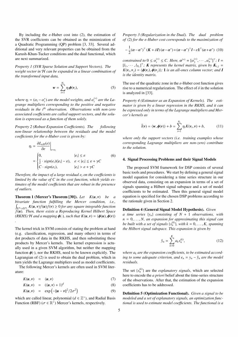
Figure 1: SVR signal model. Samples in the original input space are firstmapped to an RKHS where a linear regression is performed. All samples out-side a fixed tube of size ε are penalized, and are support vectors (double-circledsymbols). Penalization is carried out by applying (a) Vapnik’s ε-insensitive or(b) ε-Huber cost functions.
where C controls the trade-off between the regularization andthe losses. Residuals lower than ε are not penalized, whereaslarger ones have linear cost.
This cost function is a suboptimal estimator in applicationswhen combined with a regularization term [2, 47, 3] and thenoise follows a Gaussian distribution, because of the linear na-ture of the cost function. This issue has been addressed in theformulation of LS-SVM [48], where a quadratic cost is used,though in this case, sparseness of the solution is lost. An al-ternative cost function of the residuals, the ε-Huber cost, hasbeen proposed [49] by combining both the quadratic and the ε-insensitive cost. This has been shown to be a more appropriateresidual cost for SVR in general [50].
Definition 3 (ε-Huber Cost Function). The ε-Huber cost isgiven by
LεH(ei) =
0, |ei| ≤ ε12δ (|ei| − ε)2, ε ≤ |ei| ≤ eC
C(|ei| − ε) − 12δC
2, |ei| ≥ eC
(4)
where eC = ε + δC; ε is the insensitive parameter, and δ and Ccontrol the trade-off between the regularization and the losses.
The three different regions in the ε-Huber cost allow us to dealwith different kinds of noise: the ε-insensitive zone ignoresabsolute residuals lower than ε; the quadratic cost zone usesthe L2-norm of the residuals, which is appropriate for Gaussiannoise; and the linear cost zone is an efficient limit for the impactof the outliers in the optimal model coefficients. Note that (4)represents Vapnik’s ε-insensitive cost function when δ is smallenough, LS criterion for δC → ∞ and ε = 0 , and Huber’s costfunction when ε = 0 (see Fig. 1).
4
By including the ε-Huber cost into (2), the estimation ofthe SVR coefficients can be obtained as the minimization ofa Quadratic Programming (QP) problem [3, 33]. Several ad-ditional and very relevant properties can be obtained from theKarush-Khun-Tucker conditions and the dual functional, whichare next summarized.
Property 1 (SVR Sparse Solution and Support Vectors). Theweight vector inH can be expanded in a linear combination ofthe transformed input data,
w =
Nr∑i=1
ηiφ(vi), (5)
where ηi = (αi −α∗i ) are the model weights, and α(∗)
i are the La-grange multipliers corresponding to the positive and negativeresiduals in the ith observation. Observations with non-zeroassociated coefficients are called support vectors, and the solu-tion is expressed as a function of them solely.
Property 2 (Robust Expansion Coefficients). The followingnon-linear relationship between the residuals and the modelcoefficients for the ε-Huber cost is given by:
ηi =∂LεH(e)∂e
∣∣∣∣∣e=ei
=
0, |ei| ≤ ε1δ· sign(ei)(|ei| − ε), ε < |ei| ≤ ε + γC
C · sign(ei), |ei| > ε + γC
(6)
Therefore, the impact of a large residual ei on the coefficients islimited by the value of C in the cost function, which yields es-timates of the model coefficients that are robust in the presenceof outliers.
Theorem 1 (Mercer’s Theorem [30]). Let K(u, v) be abivariate function fulfilling the Mercer condition, i.e.,∫RNr×RNr K(u, v) f (u) f (v) ≥ 0 for any square integrable functionf (u). Then, there exists a Reproducing Kernel Hilbert Space(RKHS)H and a mapping φ(·), such that K(u, v) = 〈φ(u),φ(v)〉.
The kernel trick in SVM consists of stating the problem at hand(e.g. classification, regression, and many others) in terms ofdot products of data in the RKHS, and then substituting theseproducts by Mercer’s kernels. The kernel expression is actu-ally used in a given SVM algorithm, but neither the mappingfunction φ(·), nor the RKHS, need to be known explicitly. TheLagrangian of (2) is used to obtain the dual problem, which inturn yields the Lagrange multipliers used as model coefficients.
The following Mercer’s kernels are often used in SVM liter-ature:
K(u, v) = 〈u, v〉 (7)K(u, v) = (〈u, v〉 + 1)d (8)K(u, v) = exp
(−‖u − v‖2/2σ2
)(9)
which are called linear, polynomial (d ∈ Z+), and Radial BasisFunction (RBF) (σ ∈ R+) Mercer’s kernels, respectively.
Property 3 (Regularization in the Dual). The dual problemof (2) for the ε-Huber cost corresponds to the maximization of
−12
(α−α∗)> (K + δI) (α−α∗)+ (α−α∗)> l−ε1>(α+α∗) (10)
constrained to 0 ≤ α(∗)i ≤ C. Here, α(∗) = [α(∗)
1 , · · · , α(∗)n ]>; l =
[l1, · · · , lNr ]>; K represents the kernel matrix, given by Ki, j =
K(vi, v j) = 〈φ(vi),φ(v j)〉; 1 is an all-ones column vector; and Iis the identity matrix.
The use of the quadratic zone in the ε-Huber cost function givesrise to a numerical regularization. The effect of δ in the solutionis analyzed in [33].
Property 4 (Estimator as an Expansion of Kernels). The esti-mator is given by a linear regression in the RKHS, and it canbe expressed only in terms of the Lagrange multipliers and Mer-cer’s kernels as
l(v) = 〈w,φ(v)〉 + b =
Nr∑i=1
ηiK(vi, v) + b, (11)
where only the support vectors (i.e. training examples whosecorresponding Lagrange multipliers are non-zero) contributeto the solution.
4. Signal Processing Problems and their Signal Models
The proposed SVM framework for DSP consists of severalbasic tools and procedures. We start by defining a general signalmodel equation for considering a time series structure in ourobserved data, consisting on an expansion in terms of a set ofsignals spanning a Hilbert signal subspace and a set of modelcoefficients to be estimated. Then this general signal modelequation is specified for the chosen DSP problems according tothe rationale given in Section 2.
Definition 4 (General Signal Model Hypothesis). Givena time series {yn} consisting of N + 1 observations, withn = 0, . . . ,N, an expansion for approximating this signal canbe built with a set of signals {s(k)
n }, with k = 0, . . . ,K, spanningthe Hilbert signal subspace. This expansion is given by
yn =
K∑k=0
ak s(k)n , (12)
where ak are the expansion coefficients, to be estimated accord-ing to some adequate criterion, and en = yn − yn are the modelresiduals.
The set {s(k)n } are the explanatory signals, which are selected
here to encode the a priori belief about the time-series structureof the observations. After that, the estimation of the expansioncoefficients has to be addressed.
Definition 5 (Optimization Functional). Given a signal to bemodeled and a set of explanatory signals, an optimization func-tional is used to estimate model coefficients. The functional is a
5
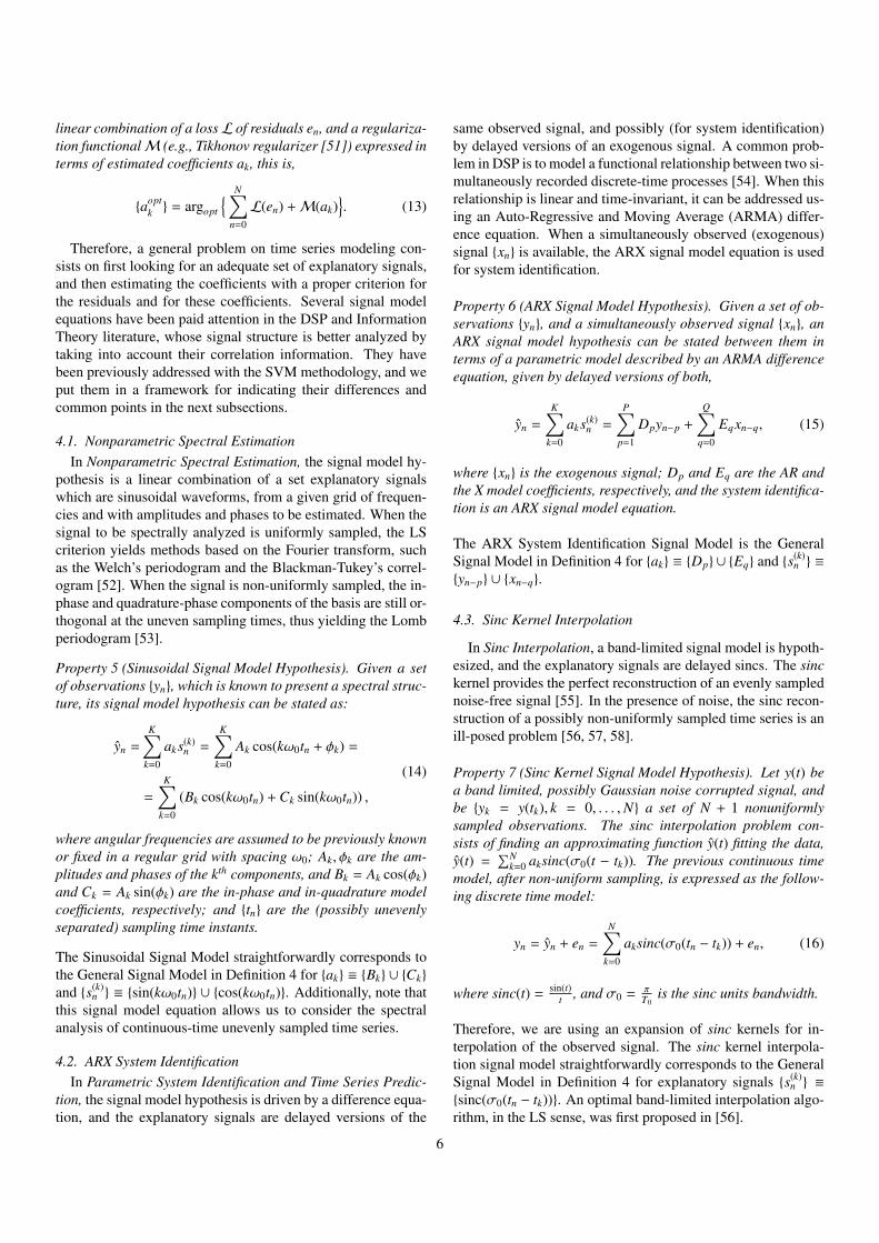
linear combination of a lossL of residuals en, and a regulariza-tion functionalM (e.g., Tikhonov regularizer [51]) expressed interms of estimated coefficients ak, this is,
{aoptk } = argopt
{ N∑n=0
L(en) +M(ak)}. (13)
Therefore, a general problem on time series modeling con-sists on first looking for an adequate set of explanatory signals,and then estimating the coefficients with a proper criterion forthe residuals and for these coefficients. Several signal modelequations have been paid attention in the DSP and InformationTheory literature, whose signal structure is better analyzed bytaking into account their correlation information. They havebeen previously addressed with the SVM methodology, and weput them in a framework for indicating their differences andcommon points in the next subsections.
4.1. Nonparametric Spectral EstimationIn Nonparametric Spectral Estimation, the signal model hy-
pothesis is a linear combination of a set explanatory signalswhich are sinusoidal waveforms, from a given grid of frequen-cies and with amplitudes and phases to be estimated. When thesignal to be spectrally analyzed is uniformly sampled, the LScriterion yields methods based on the Fourier transform, suchas the Welch’s periodogram and the Blackman-Tukey’s correl-ogram [52]. When the signal is non-uniformly sampled, the in-phase and quadrature-phase components of the basis are still or-thogonal at the uneven sampling times, thus yielding the Lombperiodogram [53].
Property 5 (Sinusoidal Signal Model Hypothesis). Given a setof observations {yn}, which is known to present a spectral struc-ture, its signal model hypothesis can be stated as:
yn =
K∑k=0
ak s(k)n =
K∑k=0
Ak cos(kω0tn + φk) =
=
K∑k=0
(Bk cos(kω0tn) + Ck sin(kω0tn)) ,
(14)
where angular frequencies are assumed to be previously knownor fixed in a regular grid with spacing ω0; Ak, φk are the am-plitudes and phases of the kth components, and Bk = Ak cos(φk)and Ck = Ak sin(φk) are the in-phase and in-quadrature modelcoefficients, respectively; and {tn} are the (possibly unevenlyseparated) sampling time instants.
The Sinusoidal Signal Model straightforwardly corresponds tothe General Signal Model in Definition 4 for {ak} ≡ {Bk} ∪ {Ck}
and {s(k)n } ≡ {sin(kω0tn)} ∪ {cos(kω0tn)}. Additionally, note that
this signal model equation allows us to consider the spectralanalysis of continuous-time unevenly sampled time series.
4.2. ARX System IdentificationIn Parametric System Identification and Time Series Predic-
tion, the signal model hypothesis is driven by a difference equa-tion, and the explanatory signals are delayed versions of the
same observed signal, and possibly (for system identification)by delayed versions of an exogenous signal. A common prob-lem in DSP is to model a functional relationship between two si-multaneously recorded discrete-time processes [54]. When thisrelationship is linear and time-invariant, it can be addressed us-ing an Auto-Regressive and Moving Average (ARMA) differ-ence equation. When a simultaneously observed (exogenous)signal {xn} is available, the ARX signal model equation is usedfor system identification.
Property 6 (ARX Signal Model Hypothesis). Given a set of ob-servations {yn}, and a simultaneously observed signal {xn}, anARX signal model hypothesis can be stated between them interms of a parametric model described by an ARMA differenceequation, given by delayed versions of both,
yn =
K∑k=0
ak s(k)n =
P∑p=1
Dpyn−p +
Q∑q=0
Eqxn−q, (15)
where {xn} is the exogenous signal; Dp and Eq are the AR andthe X model coefficients, respectively, and the system identifica-tion is an ARX signal model equation.
The ARX System Identification Signal Model is the GeneralSignal Model in Definition 4 for {ak} ≡ {Dp} ∪ {Eq} and {s(k)
n } ≡
{yn−p} ∪ {xn−q}.
4.3. Sinc Kernel Interpolation
In Sinc Interpolation, a band-limited signal model is hypoth-esized, and the explanatory signals are delayed sincs. The sinckernel provides the perfect reconstruction of an evenly samplednoise-free signal [55]. In the presence of noise, the sinc recon-struction of a possibly non-uniformly sampled time series is anill-posed problem [56, 57, 58].
Property 7 (Sinc Kernel Signal Model Hypothesis). Let y(t) bea band limited, possibly Gaussian noise corrupted signal, andbe {yk = y(tk), k = 0, . . . ,N} a set of N + 1 nonuniformlysampled observations. The sinc interpolation problem con-sists of finding an approximating function y(t) fitting the data,y(t) =
∑Nk=0 aksinc(σ0(t − tk)). The previous continuous time
model, after non-uniform sampling, is expressed as the follow-ing discrete time model:
yn = yn + en =
N∑k=0
aksinc(σ0(tn − tk)) + en, (16)
where sinc(t) =sin(t)
t , and σ0 = πT0
is the sinc units bandwidth.
Therefore, we are using an expansion of sinc kernels for in-terpolation of the observed signal. The sinc kernel interpola-tion signal model straightforwardly corresponds to the GeneralSignal Model in Definition 4 for explanatory signals {s(k)
n } ≡
{sinc(σ0(tn − tk))}. An optimal band-limited interpolation algo-rithm, in the LS sense, was first proposed in [56].
6
4.4. Sparse DeconvolutionIn Sparse Deconvolution, the signal hypothesis is given by
a convolutional signal mixture, and the explanatory signals arethe delayed and scaled versions of the impulse response from apreviously known Linear Time Invariant system. More specifi-cally, the sparse deconvolution problem consists on the estima-tion of an unknown sparse sequence which has been convolvedwith a (known) time series (impulse response of the system orsource wavelet) and corrupted by noise, hence producing theobserved noisy time series. The non-null samples of the sparseseries contain relevant information about the underlying physi-cal phenomenon in each application.
Property 8 (Sparse Deconvolution Signal Model Hypothesis).Let {yn} be a discrete-time signal given by N + 1 observedsamples of a time series, which is the result of the convolutionbetween an unknown sparse signal {xn}, to be estimated, anda known time series {hn} (with M + 1 duration). Then, thefollowing convolutional signal model equation can be written,
yn = xn ∗ hn =
M∑j=0
x jhn− j =
K∑k=0
a(k)s(k)n , (17)
where ∗ denotes the discrete-time convolution operator, and xn
is the estimation of the unknown input signal.
The Sparse Deconvolution Signal Model corresponds to theGeneral Signal Model in Definition 4 for model coefficients{ak} ≡ {xk} and explanatory signals {s(k)
n } ≡ {hn−k}. The perfor-mance of sparse deconvolution algorithms can be degraded byseveral causes. First, they can result in ill-posed problems [59],and regularization methods are often required. Also, when thenoise is non-Gaussian, either LS or maximum likelihood de-convolution can yield suboptimal solutions [60]. Finally, ifhn has non-minimum phase, some sparse deconvolution algo-rithms needing inverse filtering become unstable.
4.5. Array ProcessingIn Array Processing, a complex-valued spatio-temporal sig-
nal model equation is used in order to manage the proper-ties of an array of antennas in several signal processing ap-plications. The easiest system model in array processing [61]consists of a linear array of K + 1 elements equally spaceda distance d, whose output is a time series of vector samplesxn = {x0
n, · · · , xKn }
T or snapshots. Usually, signals xkn are repre-
sented as lowpass signals. In order to keep their amplitude andphase information, signals need a complex-valued representa-tion in terms of in-phase and quadrature-phase components. Agiven source with constant amplitude, whose direction of ar-rival (DOA) and wavelength are θl and λ, respectively, yieldsthe following array output (so-called steering vector),
al = {1, e j2π dλ sin(θl), · · · , e j2Kπ d
λ sin(θl)}>, (18)
where j =√−1. If L transmitters are present, the snapshot can
be represented as xn = Abn + nn where A is a matrix containingall steering vectors of the L transmitters, bn is a column vectorcontaining (complex valued) symbols transmitted by all usersand nn is the thermal noise present at the output of each antenna.
5 10 15 20−1
0
1
s(0)
n
5 10 15 20−1
0
1
s(1)
n
5 10 15 20−1
0
1
s(K)
n
n
s10
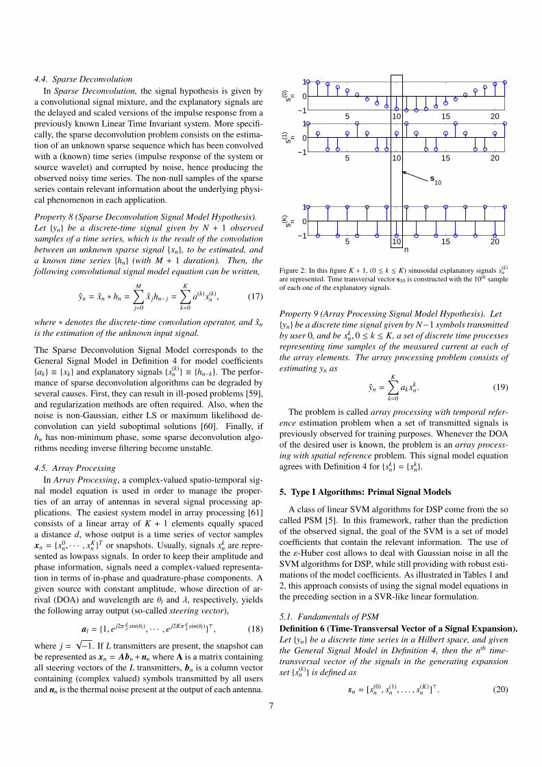
Figure 2: In this figure K + 1, (0 ≤ k ≤ K) sinusoidal explanatory signals s(k)n
are represented. Time transversal vector s10 is constructed with the 10th sampleof each one of the explanatory signals.
Property 9 (Array Processing Signal Model Hypothesis). Let{yn} be a discrete time signal given by N−1 symbols transmittedby user 0, and be xk
n, 0 ≤ k ≤ K, a set of discrete time processesrepresenting time samples of the measured current at each ofthe array elements. The array processing problem consists ofestimating yn as
yn =
K∑k=0
ak xkn. (19)
The problem is called array processing with temporal refer-ence estimation problem when a set of transmitted signals ispreviously observed for training purposes. Whenever the DOAof the desired user is known, the problem is an array process-ing with spatial reference problem. This signal model equationagrees with Definition 4 for {sk
n} = {xkn}.
5. Type I Algorithms: Primal Signal Models
A class of linear SVM algorithms for DSP come from the socalled PSM [5]. In this framework, rather than the predictionof the observed signal, the goal of the SVM is a set of modelcoefficients that contain the relevant information. The use ofthe ε-Huber cost allows to deal with Gaussian noise in all theSVM algorithms for DSP, while still providing with robust esti-mations of the model coefficients. As illustrated in Tables 1 and2, this approach consists of using the signal model equations inthe preceding section in a SVR-like linear formulation.
5.1. Fundamentals of PSMDefinition 6 (Time-Transversal Vector of a Signal Expansion).Let {yn} be a discrete time series in a Hilbert space, and giventhe General Signal Model in Definition 4, then the nth time-transversal vector of the signals in the generating expansionset {s(k)
n } is defined as
sn = [s(0)n , s(1)
n , . . . , s(K)n ]>. (20)
7

Hence, it is given by the nth samples of each of the signals gen-erating the signal subspace where the signal approximation ismade.
Figure 2 depicts a pictorial example, in which time-transversalvector s10 is given by the 10th sample of each explanatory signal(sinusoidal signals in the graph example).
Accordingly, the PSM problem can be stated as follows.
Theorem 2 (PSM Problem Statement). Let {yn} be a discretetime series in a Hilbert space, then the optimization of
12‖a‖2 +
N∑n=0
LεH(en) (21)
with a = [a0, a1, . . . , aK]>, gives an expansion solution whosesignal model equation is
yn =
K∑k=1
ak s(k)n = 〈a, sn〉 (22)
By virtue of Property 4, we can express the primal coefficientsak as
ak =
N∑n=0
ηnskn ⇒ a =
N∑n=0
ηnsn (23)
where ηn are the SVM Lagrange multipliers, and the solution atinstant m is
ym =
N∑n=0
ηn〈sn, sm〉 (24)
Only instants n with ηn , 0 are part of the solution (SupportTime Instants).
Therefore, each expansion coefficient ak can be expressed asa linear combination of input space vectors. Sparseness can beobtained in coefficients ak, but not in coefficients ηn. Robust-ness is also ensured for coefficients ak. The Lagrange multipli-ers are obtained from the dual problem, which is built in termsof a kernel matrix depending on the signal correlation.
Definition 7 (Correlation Matrix from Time-Transversal Vectors).Given the set of time-transversal vectors, the correlation matrixof the PSM is defined as
Rs(m, n) ≡ 〈sm, sn〉 =
K∑k=0
s(k)m s(k)
n (25)
In this setting, correlation matrix in Eq. (25) contains all thetemporal correlations conveyed by the explanatory signals fordifferent lags. For instance, elements in the main diagonal willconvey the zero-lag correlations between the time-transversalvectors for each time instant, whereas the upper and lower diag-onal will convey the correlations between time-transversal vec-tors for lags +1 and −1. For the particular case of s(k)
n = sn−k,thus these signals being delayed versions of a signal sn, the ma-trix is a Toeplitz matrix of the autocorrelation function of sn.In summary, this correlation matrix consists of all the lags forthe time correlations of the Hilbert signal subspace, which isalways a fundamental information when working with time se-ries.
Property 10 (Correlation Matrix and Dual Problem). Giventhe general PSM in (22) and the correlation matrix from thetime-transversal vectors in (25), the dual problem yielding theLagrange multipliers consists of maximizing
−12
(α−α∗)>(Rs + δI
)(α−α∗)+(α−α∗)>y−ε1>(α+α∗) (26)
constrained to 0 ≤ αn, α∗n ≤ C.
This property can be readily shown from considerations onthe Lagrange functional and the associated KKT conditions [5].Therefore, by taking into account the PSM for a given DSPproblem, one can determine the signals s(k)
n that generate theHilbert subspace where the observations are projected to, andthen the remaining elements and steps of the SVM methodol-ogy, such as the input space, the input space correlation matrix,the dual QP problem, and the solution, can be straightforwardlyobtained.
5.2. Spectral Analysis and System IdentificationThe first SVM algorithms for DSP that were proposed using
the PSM framework were the sinusoidal decomposition [31],the ARX system identification [33], and the γ-filter struc-ture [32]. We next point out the relevant elements that can beidentified in these algorithms.
Property 11. (PSM Coefficients for Nonparametric SpectralAnalysis). Given the signal model hypothesis for nonparamet-ric spectral analysis in Property 5, estimated coefficients usingthe PSM are
Bk =
N∑n=0
ηn cos(kω0tn); Ck =
N∑n=0
ηn sin(kω0tn). (27)
Property 12. (PSM Correlation and Dual Problem for Non-parametric Spectral Analysis). Given the signal model hypoth-esis in Property 5, the correlation matrix is given by the sum oftwo terms,
Rcos(m, n) =
K∑k=0
cos(kω0tm) cos(kω0tn) (28)
Rsin(m, n) =
K∑k=0
sin(kω0tm) sin(kω0tn) (29)
and the dual functional is given by (26) using Rs = Rcos + Rsin.
The identification of the corresponding time-transversal vec-tors is straightforward. The derivation of this algorithm in [31]is obtained by using these two properties in the PSM. Similarconsiderations can be drawn for ARX system identification al-gorithm in [33] using the next two properties.
Property 13 (PSM Coefficients for ARX System Identification).Given the signal model hypothesis for ARX system identifica-tion in Property 6, estimated PSM coefficients are
Dk =
N∑n=0
ηnyn−k; Ek =
N∑n=0
ηnxn−k+1. (30)
8
Property 14. (PSM Correlation and Dual Problem for ARXSystem Identification). Given the signal model hypothesis forARX system identification in Property 6, the correlation matrixis given by the sum of two terms,
Ry(m, n) =
P∑k=1
ym−kyn−k, (31)
Rx(m, n) =
Q∑k=0
xm−k+1xn−k+1. (32)
These equations represent the time-local Pth and Qth order sam-ple estimators of the values of the (non-Toeplitz) autocorrela-tion functions of the input and the output discrete time pro-cesses, respectively. The dual functional to be maximized isgiven by (26) using Rs = Ry + Rx.
5.3. Convolutional Signal Models
Convolutional signal model equations are those models thatcontain a convolutive mixture in their formulation. The mostrepresentative ones are the nonuniform interpolation (using sinckernels, RBF kernels, or others) and the sparse deconvolution,presented in [38, 39]. These models are relevant not only fortheir robustness, but also because their analysis gives us thefoundations of the DSM to be subsequently used in a varietyof DSP problem statements. We next focus on summarizing theproperties that are relevant for giving a signal processing blockstructure, that will be used for their analysis.
Property 15 (PSM Coefficients for Sinc Interpolation). Giventhe signal model hypothesis in Property 7 for sinc kernelinterpolation, the PSM coefficients are
ak =
N∑n=0
ηnsinc(σ0(tk − tn)). (33)
Property 16. (PSM Correlation and Dual Problem for Sinc In-terpolation). Given the signal model hypothesis in Property 7,the correlation matrix is given by
Rsinc(m, n) =
N∑k=0
sinc(σ0(tm − tk))sinc(σ0(tn − tk)) (34)
The maximized dual functional is in (26) when Rs = Rsinc.
Coefficients in (33) are proportional to the cross correlationof coefficients ηn and a set of sinc functions, each centered in-stants tn [38]. Similar considerations can be made about thesparse deconvolution signal model equation.
Property 17 (PSM Coefficients for Sparse Deconvolution).The estimated PSM coefficients of the signal model hypothesisin Property 8 are
xn =
N∑i=0
ηihi−n (35)
-
M
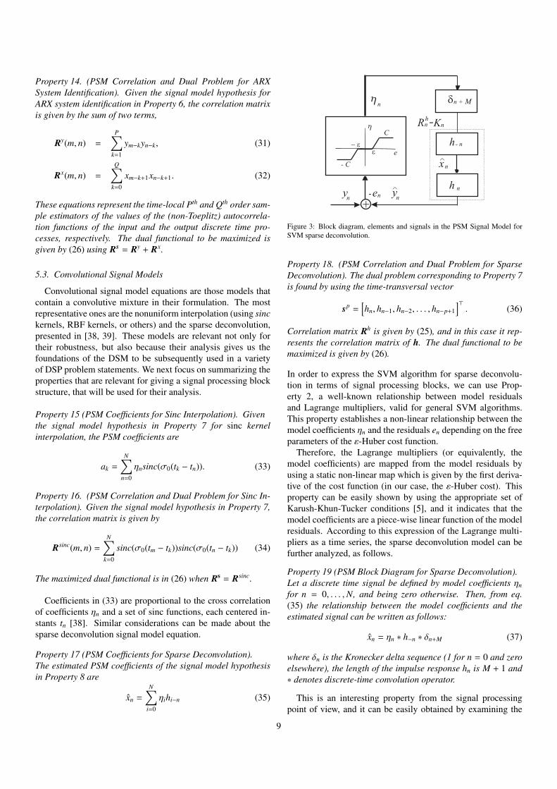
Figure 3: Block diagram, elements and signals in the PSM Signal Model forSVM sparse deconvolution.
Property 18. (PSM Correlation and Dual Problem for SparseDeconvolution). The dual problem corresponding to Property 7is found by using the time-transversal vector
sp =[hn, hn−1, hn−2, . . . , hn−p+1
]>. (36)
Correlation matrix Rh is given by (25), and in this case it rep-resents the correlation matrix of h. The dual functional to bemaximized is given by (26).
In order to express the SVM algorithm for sparse deconvolu-tion in terms of signal processing blocks, we can use Prop-erty 2, a well-known relationship between model residualsand Lagrange multipliers, valid for general SVM algorithms.This property establishes a non-linear relationship between themodel coefficients ηn and the residuals en depending on the freeparameters of the ε-Huber cost function.
Therefore, the Lagrange multipliers (or equivalently, themodel coefficients) are mapped from the model residuals byusing a static non-linear map which is given by the first deriva-tive of the cost function (in our case, the ε-Huber cost). Thisproperty can be easily shown by using the appropriate set ofKarush-Khun-Tucker conditions [5], and it indicates that themodel coefficients are a piece-wise linear function of the modelresiduals. According to this expression of the Lagrange multi-pliers as a time series, the sparse deconvolution model can befurther analyzed, as follows.
Property 19 (PSM Block Diagram for Sparse Deconvolution).Let a discrete time signal be defined by model coefficients ηn
for n = 0, . . . ,N, and being zero otherwise. Then, from eq.(35) the relationship between the model coefficients and theestimated signal can be written as follows:
xn = ηn ∗ h−n ∗ δn+M (37)
where δn is the Kronecker delta sequence (1 for n = 0 and zeroelsewhere), the length of the impulse response hn is M + 1 and∗ denotes discrete-time convolution operator.
This is an interesting property from the signal processingpoint of view, and it can be easily obtained by examining the
9
Karush-Khun-Tucker in the PSM of the sparse deconvolutionproblem [39]. Hence, we can consider a joint equivalent closed-loop system, given in Fig. 3 which contains all the elements ofthe SVM algorithm expressed as signals or systems. Specifi-cally, one is a non-linear system, given by Property 2, and theremaining ones are linear, time invariant systems. According tothe preceding property, estimated signal xn will not be sparse ingeneral, because it is the sparseness of ηn that can be controlledwith the ε parameter, but there is a convolutional relationshipbetween xn and ηn that will depend on the impulse response,which in general does not have to be sparse.
A particular class of kernels are translation invariant ker-nels, which are those fulfilling K(u, v) = K(u − v). Two highlyrelevant properties in this setting, which will be useful in thissection for PSM algorithms and later on for DSM algorithms,are the following.
Property 20 (Shift-invariant Mercer’s Kernels). A necessaryand sufficient condition for a translation invariant kernel to beMercer’s kernel [62] is that its Fourier transform must be realand non-negative, this is,
12π
∫ +∞
v=−∞
K(v)e− j2π〈 f ,v〉dv ≥ 0 ∀ f ∈ Rd (38)
Property 21 (Autocorrelation-Induced Kernel). Let {hn} be a(N + 1)-samples limited-duration discrete-time real signal, i.e.,∀n < (0,N)⇒ hn = 0, and let Rh
n = hn ∗ h−n be its autocorrela-tion function. Then, the following shift-invariant kernel can bebuilt:
Kh(n,m) = Rhn(n − m) (39)
which is called Autocorrelation-Induced Kernel (or just auto-correlation kernel). As Rh
n(m) is an even signal, its spectrum isreal and nonnegative, and according to Property 20, an auto-correlation kernel is always a Mercer’s kernel.
Now, note that there is no Mercer’s kernel appearing explic-itly in the problem statement of PSM for sparse deconvolution,as it could be expected in a SVM approach. However, the blockdiagram in Fig. 3 highlights that there is an implicitly presentautocorrelation kernel, given by
Rhn = hn ∗ h−n, (40)
in the case we associate the two systems containing the originalsystem impulse response and its reversed version. From LinearSystem Theory, the order of the blocks could be changed with-out modifying the total system. However, the solution signal isembedded between these two blocks, which precludes the ex-plicit use of this autocorrelation kernel in this PSM formulation.Finally, the role of delay system δn+M can be interpreted as justan index compensation that makes the total system causal.
In summary, the PSM algorithm yields a regularized solu-tion, in which an autocorrelation kernel is implicitly used, butit does not allow to control the sparseness of the estimated sig-nal. These properties will be used later in the DSM for highperformance sparse deconvolution algorithms.
5.4. Array Processing with Temporal Reference
The array processing algorithm needs a complex-valued for-mulation. The complex Lagrange coefficients can be expressedas ψn = ηn + jνn, ηn = αn − α
∗n and νn = βn − β
∗n being the
Lagrange coefficients generated by the real and imaginary partsof the error.
Property 22 (PSM for Array Processing). Given the array pro-cessing signal defined in Property 9, the PSM coefficients forthis problem are given by
ak =
N∑n=0
ψnxkn (41)
Property 23. (Dual Problem for Temporal Reference ArrayProcessing). Let yn, with 0 ≤ n ≤ N be a set of desired sig-nals available for training purposes, then the problem is knownas temporal reference array processing. The incoming signalkernel matrix is defined as
K(l,m) =
K∑i=0
xkl xk
m (42)
The dual functional to be maximized is a complex valued exten-sion of (26), i.e.,
ψ>Kψ + Re(ψ>y) − ε1>(α + α∗ + β + β∗), (43)
where y stands for the complex conjugate of y.
5.5. PSM Application Examples
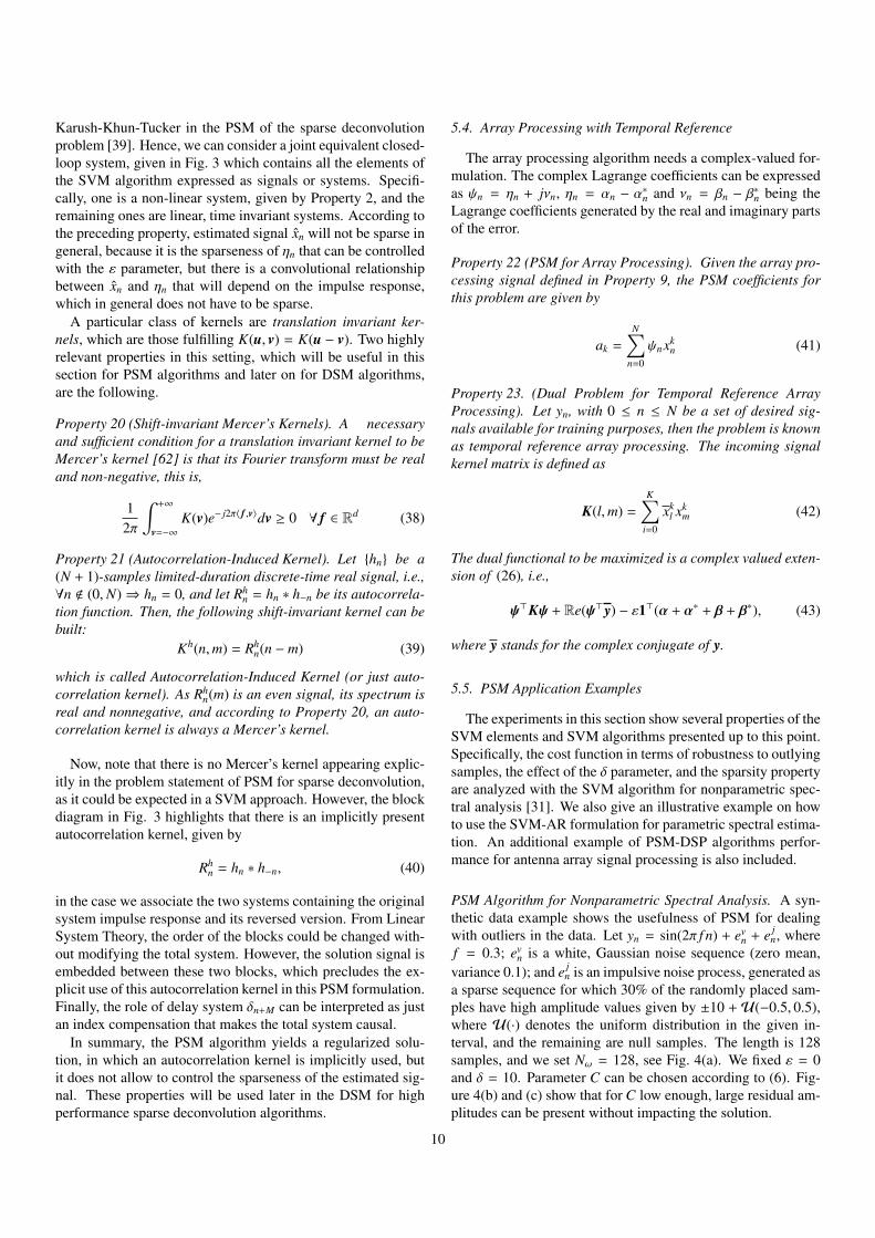
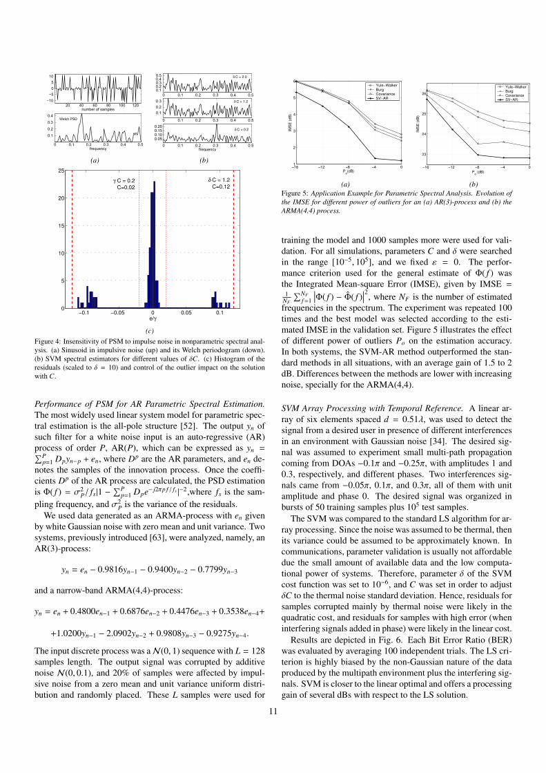
The experiments in this section show several properties of theSVM elements and SVM algorithms presented up to this point.Specifically, the cost function in terms of robustness to outlyingsamples, the effect of the δ parameter, and the sparsity propertyare analyzed with the SVM algorithm for nonparametric spec-tral analysis [31]. We also give an illustrative example on howto use the SVM-AR formulation for parametric spectral estima-tion. An additional example of PSM-DSP algorithms perfor-mance for antenna array signal processing is also included.
PSM Algorithm for Nonparametric Spectral Analysis. A syn-thetic data example shows the usefulness of PSM for dealingwith outliers in the data. Let yn = sin(2π f n) + ev
n + e jn, where
f = 0.3; evn is a white, Gaussian noise sequence (zero mean,
variance 0.1); and e jn is an impulsive noise process, generated as
a sparse sequence for which 30% of the randomly placed sam-ples have high amplitude values given by ±10 +U(−0.5, 0.5),where U(·) denotes the uniform distribution in the given in-terval, and the remaining are null samples. The length is 128samples, and we set Nω = 128, see Fig. 4(a). We fixed ε = 0and δ = 10. Parameter C can be chosen according to (6). Fig-ure 4(b) and (c) show that for C low enough, large residual am-plitudes can be present without impacting the solution.
10
20 40 60 80 100 120−10
−5
0
5
10
number of samples
0 0.1 0.2 0.3 0.4 0.5
0.1
0.2
0.3
0.4
frequency
Welch PSD
0.10.20.30.40.5
0.1
0.2
0.3
0.050.100.150.20
frequency
δC = 2.0
δC = 1.2
δC = 0.2
0 0.1 0.2 0.3 0.4 0.5
0 0.1 0.2 0.3 0.4 0.5
0 0.1 0.2 0.3 0.4 0.5
(a) (b)
−0.1 −0.05 0 0.05 0.10
5
10
15
20
25
e/γ
γ C = 0.2 C=0.02
δ C = 1.2 C=0.12
(c)Figure 4: Insensitivity of PSM to impulse noise in nonparametric spectral anal-ysis. (a) Sinusoid in impulsive noise (up) and its Welch periodogram (down).(b) SVM spectral estimators for different values of δC. (c) Histogram of theresiduals (scaled to δ = 10) and control of the outlier impact on the solutionwith C.
Performance of PSM for AR Parametric Spectral Estimation.The most widely used linear system model for parametric spec-tral estimation is the all-pole structure [52]. The output yn ofsuch filter for a white noise input is an auto-regressive (AR)process of order P, AR(P), which can be expressed as yn =∑P
p=1 Dpyn−p + en, where Dp are the AR parameters, and en de-notes the samples of the innovation process. Once the coeffi-cients Dp of the AR process are calculated, the PSD estimationis Φ( f ) = σ2
P/ fs|1 −∑P
p=1 Dpe− j2πp f / fs |−2,where fs is the sam-pling frequency, and σ2
P is the variance of the residuals.We used data generated as an ARMA-process with en given
by white Gaussian noise with zero mean and unit variance. Twosystems, previously introduced [63], were analyzed, namely, anAR(3)-process:
yn = en − 0.9816yn−1 − 0.9400yn−2 − 0.7799yn−3
and a narrow-band ARMA(4,4)-process:
yn = en + 0.4800en−1 + 0.6876en−2 + 0.4476en−3 + 0.3538en−4+
+1.0200yn−1 − 2.0902yn−2 + 0.9808yn−3 − 0.9275yn−4.
The input discrete process was aN(0, 1) sequence with L = 128samples length. The output signal was corrupted by additivenoise N(0, 0.1), and 20% of samples were affected by impul-sive noise from a zero mean and unit variance uniform distri-bution and randomly placed. These L samples were used for
−16 −12 −8 −4 01
2
3
4
5
6
Po(dB)
IMSE(dB)
Yule−WalkerBurgCovarianceSV−AR
−16 −12 −8 −4 0
23
24
25
26
Po(dB)
IMSE(dB)
Yule−WalkerBurgCovarianceSV−AR
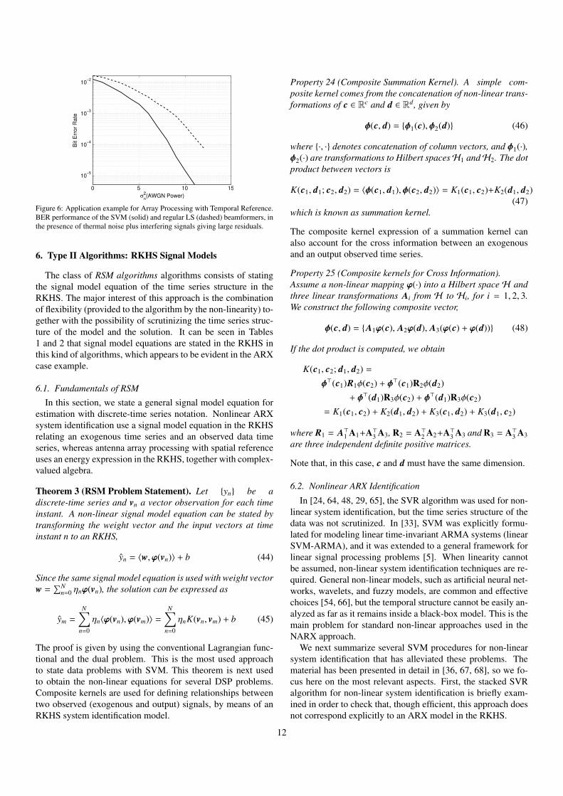
(a) (b)Figure 5: Application Example for Parametric Spectral Analysis. Evolution ofthe IMSE for different power of outliers for an (a) AR(3)-process and (b) theARMA(4,4) process.
training the model and 1000 samples more were used for vali-dation. For all simulations, parameters C and δ were searchedin the range [10−5, 105], and we fixed ε = 0. The perfor-mance criterion used for the general estimate of Φ( f ) wasthe Integrated Mean-square Error (IMSE), given by IMSE =
1NF
∑NFf =1
∣∣∣Φ( f ) − Φ( f )∣∣∣2, where NF is the number of estimated
frequencies in the spectrum. The experiment was repeated 100times and the best model was selected according to the esti-mated IMSE in the validation set. Figure 5 illustrates the effectof different power of outliers Po on the estimation accuracy.In both systems, the SVM-AR method outperformed the stan-dard methods in all situations, with an average gain of 1.5 to 2dB. Differences between the methods are lower with increasingnoise, specially for the ARMA(4,4).
SVM Array Processing with Temporal Reference. A linear ar-ray of six elements spaced d = 0.51λ, was used to detect thesignal from a desired user in presence of different interferencesin an environment with Gaussian noise [34]. The desired sig-nal was assumed to experiment small multi-path propagationcoming from DOAs −0.1π and −0.25π, with amplitudes 1 and0.3, respectively, and different phases. Two interferences sig-nals came from −0.05π, 0.1π, and 0.3π, all of them with unitamplitude and phase 0. The desired signal was organized inbursts of 50 training samples plus 105 test samples.
The SVM was compared to the standard LS algorithm for ar-ray processing. Since the noise was assumed to be thermal, thenits variance could be assumed to be approximately known. Incommunications, parameter validation is usually not affordabledue the small amount of available data and the low computa-tional power of systems. Therefore, parameter δ of the SVMcost function was set to 10−6, and C was set in order to adjustδC to the thermal noise standard deviation. Hence, residuals forsamples corrupted mainly by thermal noise were likely in thequadratic cost, and residuals for samples with high error (wheninterfering signals added in phase) were likely in the linear cost.
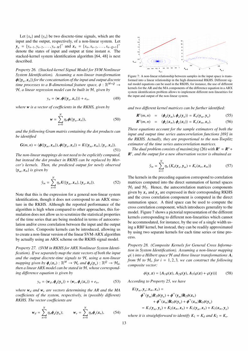
Results are depicted in Fig. 6. Each Bit Error Ratio (BER)was evaluated by averaging 100 independent trials. The LS cri-terion is highly biased by the non-Gaussian nature of the dataproduced by the multipath environment plus the interfering sig-nals. SVM is closer to the linear optimal and offers a processinggain of several dBs with respect to the LS solution.
11
σn2(AWGN Power)
0 5 10 15
Bit
Err
orR
ate
10−5
10−4
10−3
10−2
Figure 6: Application example for Array Processing with Temporal Reference.BER performance of the SVM (solid) and regular LS (dashed) beamformers, inthe presence of thermal noise plus interfering signals giving large residuals.
6. Type II Algorithms: RKHS Signal Models
The class of RSM algorithms algorithms consists of statingthe signal model equation of the time series structure in theRKHS. The major interest of this approach is the combinationof flexibility (provided to the algorithm by the non-linearity) to-gether with the possibility of scrutinizing the time series struc-ture of the model and the solution. It can be seen in Tables1 and 2 that signal model equations are stated in the RKHS inthis kind of algorithms, which appears to be evident in the ARXcase example.
6.1. Fundamentals of RSM
In this section, we state a general signal model equation forestimation with discrete-time series notation. Nonlinear ARXsystem identification use a signal model equation in the RKHSrelating an exogenous time series and an observed data timeseries, whereas antenna array processing with spatial referenceuses an energy expression in the RKHS, together with complex-valued algebra.
Theorem 3 (RSM Problem Statement). Let {yn} be adiscrete-time series and vn a vector observation for each timeinstant. A non-linear signal model equation can be stated bytransforming the weight vector and the input vectors at timeinstant n to an RKHS,
yn = 〈w,ϕ(vn)〉 + b (44)
Since the same signal model equation is used with weight vectorw =
∑Nn=0 ηnϕ(vn), the solution can be expressed as
ym =
N∑n=0
ηn〈ϕ(vn),ϕ(vm)〉 =
N∑n=0
ηnK(vn, vm) + b (45)
The proof is given by using the conventional Lagrangian func-tional and the dual problem. This is the most used approachto state data problems with SVM. This theorem is next usedto obtain the non-linear equations for several DSP problems.Composite kernels are used for defining relationships betweentwo observed (exogenous and output) signals, by means of anRKHS system identification model.
Property 24 (Composite Summation Kernel). A simple com-posite kernel comes from the concatenation of non-linear trans-formations of c ∈ Rc and d ∈ Rd, given by
φ(c, d) = {φ1(c),φ2(d)} (46)
where {·, ·} denotes concatenation of column vectors, and φ1(·),φ2(·) are transformations to Hilbert spacesH1 andH2. The dotproduct between vectors is
K(c1, d1; c2, d2) = 〈φ(c1, d1),φ(c2, d2)〉 = K1(c1, c2)+K2(d1, d2)(47)
which is known as summation kernel.
The composite kernel expression of a summation kernel canalso account for the cross information between an exogenousand an output observed time series.
Property 25 (Composite kernels for Cross Information).Assume a non-linear mapping ϕ(·) into a Hilbert space H andthree linear transformations Ai from H to Hi, for i = 1, 2, 3.We construct the following composite vector,
φ(c, d) = {A1ϕ(c), A2ϕ(d), A3(ϕ(c) + ϕ(d))} (48)
If the dot product is computed, we obtain
K(c1, c2; d1, d2) =
φ>(c1)R1φ(c2) + φ>(c1)R2φ(d2)+ φ>(d1)R3φ(c2) + φ>(d1)R3φ(c2)
= K1(c1, c2) + K2(d1, d2) + K3(c1, d2) + K3(d1, c2)
where R1 = A>1 A1+A>3 A3, R2 = A>2 A2+A>3 A3 and R3 = A>3 A3are three independent definite positive matrices.
Note that, in this case, c and d must have the same dimension.
6.2. Nonlinear ARX Identification
In [24, 64, 48, 29, 65], the SVR algorithm was used for non-linear system identification, but the time series structure of thedata was not scrutinized. In [33], SVM was explicitly formu-lated for modeling linear time-invariant ARMA systems (linearSVM-ARMA), and it was extended to a general framework forlinear signal processing problems [5]. When linearity cannotbe assumed, non-linear system identification techniques are re-quired. General non-linear models, such as artificial neural net-works, wavelets, and fuzzy models, are common and effectivechoices [54, 66], but the temporal structure cannot be easily an-alyzed as far as it remains inside a black-box model. This is themain problem for standard non-linear approaches used in theNARX approach.
We next summarize several SVM procedures for non-linearsystem identification that has alleviated these problems. Thematerial has been presented in detail in [36, 67, 68], so we fo-cus here on the most relevant aspects. First, the stacked SVRalgorithm for non-linear system identification is briefly exam-ined in order to check that, though efficient, this approach doesnot correspond explicitly to an ARX model in the RKHS.
12
Let {xn} and {yn} be two discrete-time signals, which are theinput and the output, respectively, of a non-linear system. Letyn = [yn−1, yn−2, . . . , yn−M]> and xn = [xn, xn−1, . . . , xn−Q+1]>
denote the states of input and output at time instant n. Thestacked-kernel system identification algorithm [64, 48] is nextdescribed.
Property 26. (Stacked-kernel Signal Model for SVM NonlinearSystem Identification). Assuming a non-linear transformationφ({yn, xn}) for the concatenation of the input and output discretetime processes to a B-dimensional feature space, φ : RM+Q →
H , a linear regression model can be built inH , given by
yn = 〈w,φ({yn, xn})〉 + en, (49)
where w is a vector of coefficients in the RKHS, given by
w =
N∑n=0
ηnφ({yn, xn}), (50)
and the following Gram matrix containing the dot products canbe identified
G(m, n) = 〈φ({ym, xm}),φ({yn, xn}) = K({ym, xm}, {yn, xn}).(51)
The non-linear mappings do not need to be explicitly computed,but instead the dot product in RKHS can be replaced by Mer-cer’s kernels. Then, the predicted output for newly observed{ym, xm} is given by
ym =
N∑n=0
ηnK({ym, xm}, {yn, xn}). (52)
Note that this is the expression for a general non-linear systemidentification, though it does not correspond to an ARX struc-ture in the RKHS. Although the reported performance of thealgorithm is high when compared to other approaches, this for-mulation does not allow us to scrutinize the statistical propertiesof the time series that are being modeled in terms of autocorre-lation and/or cross correlation between the input and the outputtime series. Composite kernels can be introduced, allowing usto create a non-linear version of the linear SVM-ARX algorithmby actually using an ARX scheme on the RKHS signal model.
Property 27. (SVM in RKHS for ARX Nonlinear System Identi-fication). If we separately map the state vectors of both the inputand the output discrete-time signals to H , using a non-linearmapping given by φe(xn) : RM → He and φd(yn) : RQ → Hd,then a linear ARX model can be stated inH , whose correspond-ing difference equation is given by
yn = 〈wd,φd(yn)〉 + 〈we,φe(xn)〉 + en, (53)
where wd and we are vectors determining the AR and the MAcoefficients of the system, respectively, in (possibly different)RKHS. The vector coefficients are
wd =
N∑n=0
ηnφd(yn); we =
N∑n=0
ηnφe(xn), (54)
−0.6 −0.4 −0.2 0 0.2 0.4 0.6 0.8 1−0.5
0
0.5
0
0.5
1
1.5
2
2.5
3
3.5
yn−1
yn−2
0
0.5
1
0
0.5
10
2
4
6
8
10
12
xn−1
xn−2
Figure 7: A non-linear relationship between samples in the input space is trans-formed into a linear relationship in the high dimensional RKHS. Different sig-nal model equations can be used in the RKHS, for instance, the use of differentkernels for the AR and the MA components of the difference equation in a ARXsystem identification problem allows to implement different non-linearities forthe input and output of the non-linear system.
and two different kernel matrices can be further identified:
Ry(m, n) = 〈φd(ym),φd(yn)〉 = Kd(ym, yn) (55)Rx(m, n) = 〈φe(xm),φe(xk)〉 = Ke(xm, xn). (56)
These equations account for the sample estimators of both theinput and output time series autocorrelation functions [69] inthe RKHS. Actually, they are proportional to the non-Toeplitzestimator of the time series autocorrelation matrices.
The dual problem consists of maximizing (26) with Rs = Rx+
Ry, and the output for a new observation vector is obtained as
ym =
N∑n=1
ηn(Kd(yn, ym) + Ke(xn, xm)
)(57)
The kernels in the preceding equation correspond to correlationmatrices computed into the direct summation of kernel spacesH1 and H2. Hence, the autocorrelation matrices componentsgiven by xn and yn are expressed in their corresponding RKHSand the cross correlation component is computed in the directsummation space. A third space can be used to compute thecross correlation component, which introduces generality to themodel. Figure 7 shows a pictorial representation of the differentkernels corresponding to different non-linearities which cannotbe accommodated, for instance, by the use of a single width us-ing a RBF kernel, but instead, they can be readily approximatedby using two separate kernels for each time series or time pro-cess.
Property 28. (Composite Kernels for General Cross Informa-tion in System Identification). Assuming a non-linear mappingϕ(·) into a Hilbert spaceH and three linear transformations Ai
from H to Hi, for i = 1, 2, 3, we can construct the followingcomposite vector:
φ(y, x) = {A1ϕ(x), A2ϕ(y), A3(ϕ(x) + ϕ(y))} (58)
According to Property 25, we have
K(ym, yn; xm, xn) =
φ>(ym)R1φ(yn) + φ>(ym)R2φ(xn)+ φ>(xm)R3φ(yn) + φ>(xm)R3φ(yn)
= K1(ym, yn) + K2(xm, xn) + K3(ym, xn) + K3(xm, yn)
where it is straightforward to identify K1 = Kd and K2 = Ke.
13
Note that in this case, xn and yn need to have the same dimen-sion, which can be naively accomplished by zero completion ofthe embeddings.
Property 29 (General Composite Kernels). A general compos-ite kernel, that can be obtained as a combination of the previousones, is given by
K(xm, ym; yn, xn) = K1(ym, yn) + K2(xm, xn)+ K3(ym, xn) + K3(xm, yn) + K4(zm, zn)
(59)
Therefore, despite the fact of SVM-ARX and SVR non-linearsystem identification are different problem statements, bothmodels can be easily combined.
6.3. Array Processing with Spatial ReferenceThe array processing problem stated in (19) can be solved
when there are no training symbols available, but just a set ofincoming data and information about the angle of arrival of thedesired user. In this case, the algorithm to be applied consists ofa processor that detects without distortion (distortionless prop-erty) the signal from the desired direction of arrival while mini-mizing the total output energy. The signal can be easily mappedto an RKHS, and then we minimize
E = E(wHϕ(xn)ϕ(xn)Hw) = wH Rw ≈ wHΦΦHw (60)
for a given set of previously collected snapshots, where Estands for statistical expectation, and Φ is a matrix containingall mapped snapshots ϕ(xn).
Property 30 (Spatial Reference Signal Model in RKHS). In or-der to introduce the distortionless property, constraints mustbe applied to a set of canonical signals (spatial reference sig-nals) whose steering vector (18) contains the desired directionof arrival θ0, carrying a set of symbols bi. The reference signalmodel equation is
bi = wHϕ(bia0) − b (61)
where a0 is the steering vector corresponding to the desiredsignal. Then, a primal functional must contain the followingconstraints
Re(bi − wHϕ(bia0) − b
)≤ ε + ξi
−Re(bi − wHϕ(bia0) − b
)≤ ε + ξ′i
Im(bi − wHϕ(bia0) − b
)≤ ε + ζi
−Im(bi − wHϕ(bia0) − b
)≤ ε + ζ′i
(62)
being si all possible transmitted symbols in a given amplituderange, and ξi, ζi, ξ
′i , ζ′i the slack variables corresponding to the
real and imaginary constraints.
Property 31 (Spatial Reference primal coefficients). A SVMprocedure applied to this constrained optimization problemhas to minimize (61), and it gives
w =∑
i
R−1ϕ(bia0)ψi (63)
+
-
Lorenz attractor
Non-linear feeback system
Low-pass filterH(z)
High-pass filterG(z)
f(·)=log(·)
−20 −10 0 10 200
10
20
30
40
50
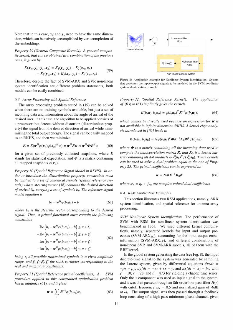
Figure 8: Application example for Nonlinear System Identification. Systemthat generates the input-output signals to be modeled in the SVM non-linearsystem identification example.
Property 32. (Spatial Reference Kernel). The applicationof (63) in (61) implicitly gives the kernels
K(bia0, b ja0) = ϕ(bia0)T R−1ϕ(b ja0), (64)
which cannot be directly used because an expression for R isnot available in infinite dimension RKHS. A kernel eigenanaly-sis introduced in [70] leads to
K(bia0, b ja0) = Nϕ(bia0)TΦK−1K0ΦTϕ(b ja0), (65)
where Φ is a matrix containing all the incoming data used tocompute the autocorrelation matrix R, and K0 is a kernel ma-trix containing all dot products ϕ(s0
na0)>ϕ(s0ma0). These kernels
can be used to solve a dual problem equal to the one of Prop-erty 23. The primal coefficients can be expressed as
w = NΦK−1K0ψ (66)
where ψn = ηn + jνn are complex-valued dual coefficients.
6.4. RSM Application Examples
This section illustrates two RSM applications, namely, ARXsystem identification, and spatial reference for antenna arrayprocessing.
SVM Nonlinear System Identification. The performance ofSVM with RSM for non-linear system identification wasbenchmarked in [36]. We used different kernel combina-tions, namely, separated kernels for input and output pro-cesses (SVM-ARX2K), accounting for the input-output cross-information (SVM-ARX4K), and different combinations ofnon-linear SVR and SVM-ARX models, all of them with theRBF kernel.
In the global system generating the data (see Fig. 8), the inputdiscrete-time signal to the system was generated by samplingthe Lorenz system, given by differential equations dx/dt =
−ρx + ρy, dy/dt = −xz + rx − y, and dx/dt = xy − bz, withρ = 10, r = 28, and b = 8/3 for yielding a chaotic time series.Only the x component was used as input signal to the system,and it was then passed through an 8th-order low-pass filter H(z)with cutoff frequency ωn = 0.5 and normalized gain of -6dBat ωn. The output signal was then passed through a feedbackloop consisting of a high-pass minimum-phase channel, given
14

Table 3: Mean error (ME), mean-squared error (MSE), mean absolute error(MAE), and correlation coefficient (r) of models in the test set.
ME MSE MAE rSVR 0.05 30.37 4.63 0.76SVM-ARX2K -0.21 39.77 5.11 0.94SVM-ARX4K 2.95 20.64 2.99 0.96SVR + SVM-ARX2K -0.00 0.01 0.07 0.99SVR + SVM-ARX4K 0.03 0.02 0.11 0.99
by on = gn − 2.01on−1 − 1.46on−2 − 0.39on−3, where on and gn
denote the input and the output signals to the channel. Outputon was distorted with f (·) = log(·).
We generated 1000 input-output sets of observations andthese were split into a cross-validation dataset (free parameterselection, 100 samples) and a test set (model performance, fol-lowing 500 samples). The experiment was repeated 100 timeswith randomly selected starting points, and the free parame-ters were adjusted with cross-validation in all the experiments.Table 3 shows the averaged results. The best models were ob-tained when combining SVR and SVM-ARX models, thoughno numerical differences were observed between SVR+SVM-ARX2K and SVR+SVM-ARX2K . In this example, all modelsconsidering cross-terms in the kernels significantly improvedSVR results.
Spatial and Temporal Antenna Array Kernel Processing. Thekernel temporal reference (SVM-TR) and spatial reference(SVM-SR) array processors have been benchmarked with theirkernel LS counterparts (kernel-TR and kernel-SR), with the lin-ear with temporal reference (MMSE), and with spatial refer-ence (MVDM) [36] . A Gaussian kernel was used in all proces-sors. The scenario consisted of a multiuser environment withone desired three interfering users. The modulated signals wereindependent QPSK, and the noise was assumed to be thermal,simulated by additive white Gaussian noise. The desired signalwas structured in bursts containing 100 training symbols, fol-lowed by 1000 test symbols. Free parameters were chosen inthe first experiment and fixed.
In the first experiment, the BER is measured as a functionof kernel parameter δ for arrays of 5 and 7 elements, in an en-vironment of three interferences from angles of arrival of 10o,20o and −10o, and unitary amplitudes, while the desired signalcame from an angle of arrival of 0o with the same amplitudeas the interferences. Results in Figure 9 show the BER as afunction of the RBF kernel width for the temporal and spatialreference SVM algorithms (i.e. SVM-TR and SVM-SR). Theseresults are compared to the temporal and spatial kernel LS al-gorithms (i.e., KLS-TR and KLS-SR), and for 7 and 5 array-elements. The noise power is of −1 dB for 7 elements and -6dB for 5 elements.
The results of the second experiment are shown in Fig. 10.The experiment measured the BER of the four non-linear pro-cessors as a function of the thermal noise power in an envi-ronment with three interfering signals from angles of arrival of−10o, 10o and 20o. Desired signal direction of arrival was 0o.
SVM LS
100 10110−3
10−2
10−1
100
b
BER
100 10110−3
10−2
10−1
100
b
BER
100 101
10−4
10−3
10−2
10−1
100
b
BER
100 101
10−4
10−3
10−2
10−1
100
b
BER
Figure 9: Application example for Spatial and Temporal Antenna Array kernelprocessing. BER performance, as a function of Gaussian RBF kernel parameterδ, of the TR (squares) and the SR (circles) in an array of 7 (top) and 5 (bottom)elements and with three interfering signals. Continuous line corresponds to theperformance of the linear algorithms.
1 2 3 4 5 610−6
10−5
10−4
10−3
10−2
10−1
−10log10m2
BER
Linear LS TRLinear MVDR SRSVM−TRKLS−TRSVM−SRKLS−SR
Figure 10: BER performance as a function of thermal noise power for linearalgorithms, SVM SVM-TR, SVM-SR, KLS-TR and KLS-SR.
Performances are compared to the linear MVDR and MMSEalgorithms. In this experiment, temporal reference algorithmsshow a performance slightly better than spatial reference ones.All non-linear approaches show an improvement of severaldecibels with respect to the linear algorithms. In particular,SVM approaches show better performance than non-linear LSalgorithms, with lower test computational burden due to theirsparseness properties.
7. Type III Algorithms: Dual Signal Models
An additional class of non-linear SVM algorithms for DSPcan be obtained by considering the non-linear regression of thetime lags or the time instants of the observed signals and us-ing an appropriate choice of the Mercer’s kernel. This class isknown as DSM based SVM algorithms. Here, we summarizethis approach and pay attention to the interesting and simpleinterpretation of these SVM algorithms under study in connec-
15
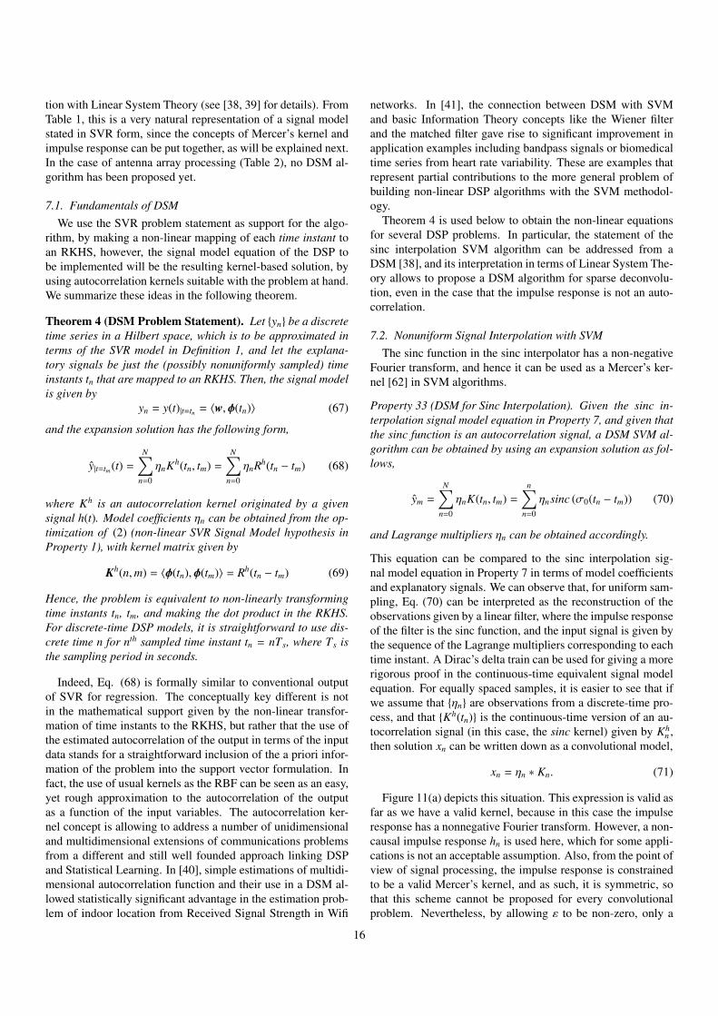
tion with Linear System Theory (see [38, 39] for details). FromTable 1, this is a very natural representation of a signal modelstated in SVR form, since the concepts of Mercer’s kernel andimpulse response can be put together, as will be explained next.In the case of antenna array processing (Table 2), no DSM al-gorithm has been proposed yet.
7.1. Fundamentals of DSMWe use the SVR problem statement as support for the algo-
rithm, by making a non-linear mapping of each time instant toan RKHS, however, the signal model equation of the DSP tobe implemented will be the resulting kernel-based solution, byusing autocorrelation kernels suitable with the problem at hand.We summarize these ideas in the following theorem.
Theorem 4 (DSM Problem Statement). Let {yn} be a discretetime series in a Hilbert space, which is to be approximated interms of the SVR model in Definition 1, and let the explana-tory signals be just the (possibly nonuniformly sampled) timeinstants tn that are mapped to an RKHS. Then, the signal modelis given by
yn = y(t)|t=tn = 〈w,φ(tn)〉 (67)
and the expansion solution has the following form,
y|t=tm (t) =
N∑n=0
ηnKh(tn, tm) =
N∑n=0
ηnRh(tn − tm) (68)
where Kh is an autocorrelation kernel originated by a givensignal h(t). Model coefficients ηn can be obtained from the op-timization of (2) (non-linear SVR Signal Model hypothesis inProperty 1), with kernel matrix given by
Kh(n,m) = 〈φ(tn),φ(tm)〉 = Rh(tn − tm) (69)
Hence, the problem is equivalent to non-linearly transformingtime instants tn, tm, and making the dot product in the RKHS.For discrete-time DSP models, it is straightforward to use dis-crete time n for nth sampled time instant tn = nTs, where Ts isthe sampling period in seconds.
Indeed, Eq. (68) is formally similar to conventional outputof SVR for regression. The conceptually key different is notin the mathematical support given by the non-linear transfor-mation of time instants to the RKHS, but rather that the use ofthe estimated autocorrelation of the output in terms of the inputdata stands for a straightforward inclusion of the a priori infor-mation of the problem into the support vector formulation. Infact, the use of usual kernels as the RBF can be seen as an easy,yet rough approximation to the autocorrelation of the outputas a function of the input variables. The autocorrelation ker-nel concept is allowing to address a number of unidimensionaland multidimensional extensions of communications problemsfrom a different and still well founded approach linking DSPand Statistical Learning. In [40], simple estimations of multidi-mensional autocorrelation function and their use in a DSM al-lowed statistically significant advantage in the estimation prob-lem of indoor location from Received Signal Strength in Wifi
networks. In [41], the connection between DSM with SVMand basic Information Theory concepts like the Wiener filterand the matched filter gave rise to significant improvement inapplication examples including bandpass signals or biomedicaltime series from heart rate variability. These are examples thatrepresent partial contributions to the more general problem ofbuilding non-linear DSP algorithms with the SVM methodol-ogy.
Theorem 4 is used below to obtain the non-linear equationsfor several DSP problems. In particular, the statement of thesinc interpolation SVM algorithm can be addressed from aDSM [38], and its interpretation in terms of Linear System The-ory allows to propose a DSM algorithm for sparse deconvolu-tion, even in the case that the impulse response is not an auto-correlation.
7.2. Nonuniform Signal Interpolation with SVMThe sinc function in the sinc interpolator has a non-negative
Fourier transform, and hence it can be used as a Mercer’s ker-nel [62] in SVM algorithms.
Property 33 (DSM for Sinc Interpolation). Given the sinc in-terpolation signal model equation in Property 7, and given thatthe sinc function is an autocorrelation signal, a DSM SVM al-gorithm can be obtained by using an expansion solution as fol-lows,
ym =
N∑n=0
ηnK(tn, tm) =
n∑n=0
ηnsinc (σ0(tn − tm)) (70)
and Lagrange multipliers ηn can be obtained accordingly.
This equation can be compared to the sinc interpolation sig-nal model equation in Property 7 in terms of model coefficientsand explanatory signals. We can observe that, for uniform sam-pling, Eq. (70) can be interpreted as the reconstruction of theobservations given by a linear filter, where the impulse responseof the filter is the sinc function, and the input signal is given bythe sequence of the Lagrange multipliers corresponding to eachtime instant. A Dirac’s delta train can be used for giving a morerigorous proof in the continuous-time equivalent signal modelequation. For equally spaced samples, it is easier to see that ifwe assume that {ηn} are observations from a discrete-time pro-cess, and that {Kh(tn)} is the continuous-time version of an au-tocorrelation signal (in this case, the sinc kernel) given by Kh
n ,then solution xn can be written down as a convolutional model,
xn = ηn ∗ Kn. (71)
Figure 11(a) depicts this situation. This expression is valid asfar as we have a valid kernel, because in this case the impulseresponse has a nonnegative Fourier transform. However, a non-causal impulse response hn is used here, which for some appli-cations is not an acceptable assumption. Also, from the point ofview of signal processing, the impulse response is constrainedto be a valid Mercer’s kernel, and as such, it is symmetric, sothat this scheme cannot be proposed for every convolutionalproblem. Nevertheless, by allowing ε to be non-zero, only a
16
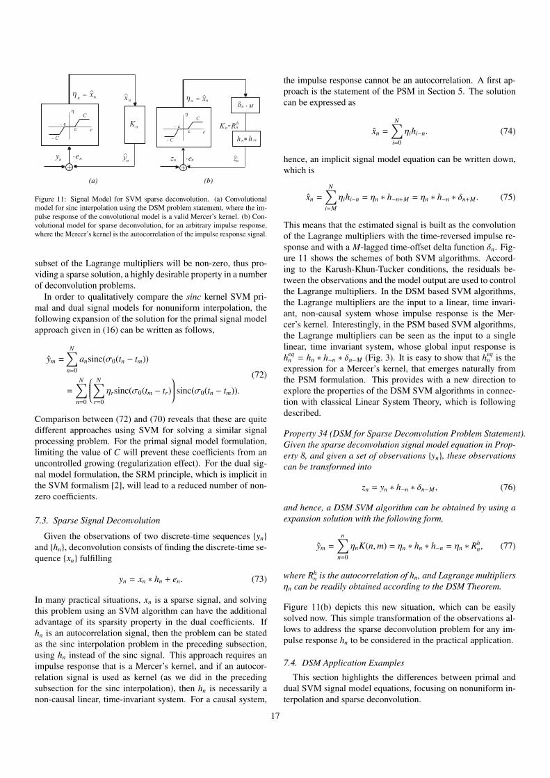
- -
M
(a) (b)
Figure 11: Signal Model for SVM sparse deconvolution. (a) Convolutionalmodel for sinc interpolation using the DSM problem statement, where the im-pulse response of the convolutional model is a valid Mercer’s kernel. (b) Con-volutional model for sparse deconvolution, for an arbitrary impulse response,where the Mercer’s kernel is the autocorrelation of the impulse response signal.
subset of the Lagrange multipliers will be non-zero, thus pro-viding a sparse solution, a highly desirable property in a numberof deconvolution problems.
In order to qualitatively compare the sinc kernel SVM pri-mal and dual signal models for nonuniform interpolation, thefollowing expansion of the solution for the primal signal modelapproach given in (16) can be written as follows,
ym =
N∑n=0
ansinc(σ0(tn − tm))
=
N∑n=0
N∑r=0
ηrsinc(σ0(tm − tr)
sinc(σ0(tn − tm)).
(72)
Comparison between (72) and (70) reveals that these are quitedifferent approaches using SVM for solving a similar signalprocessing problem. For the primal signal model formulation,limiting the value of C will prevent these coefficients from anuncontrolled growing (regularization effect). For the dual sig-nal model formulation, the SRM principle, which is implicit inthe SVM formalism [2], will lead to a reduced number of non-zero coefficients.
7.3. Sparse Signal Deconvolution
Given the observations of two discrete-time sequences {yn}
and {hn}, deconvolution consists of finding the discrete-time se-quence {xn} fulfilling
yn = xn ∗ hn + en. (73)
In many practical situations, xn is a sparse signal, and solvingthis problem using an SVM algorithm can have the additionaladvantage of its sparsity property in the dual coefficients. Ifhn is an autocorrelation signal, then the problem can be statedas the sinc interpolation problem in the preceding subsection,using hn instead of the sinc signal. This approach requires animpulse response that is a Mercer’s kernel, and if an autocor-relation signal is used as kernel (as we did in the precedingsubsection for the sinc interpolation), then hn is necessarily anon-causal linear, time-invariant system. For a causal system,
the impulse response cannot be an autocorrelation. A first ap-proach is the statement of the PSM in Section 5. The solutioncan be expressed as
xn =
N∑i=0
ηihi−n. (74)
hence, an implicit signal model equation can be written down,which is
xn =
N∑i=M
ηihi−n = ηn ∗ h−n+M = ηn ∗ h−n ∗ δn+M . (75)
This means that the estimated signal is built as the convolutionof the Lagrange multipliers with the time-reversed impulse re-sponse and with a M-lagged time-offset delta function δn. Fig-ure 11 shows the schemes of both SVM algorithms. Accord-ing to the Karush-Khun-Tucker conditions, the residuals be-tween the observations and the model output are used to controlthe Lagrange multipliers. In the DSM based SVM algorithms,the Lagrange multipliers are the input to a linear, time invari-ant, non-causal system whose impulse response is the Mer-cer’s kernel. Interestingly, in the PSM based SVM algorithms,the Lagrange multipliers can be seen as the input to a singlelinear, time invariant system, whose global input response isheq
n = hn ∗ h−n ∗ δn−M (Fig. 3). It is easy to show that heqn is the
expression for a Mercer’s kernel, that emerges naturally fromthe PSM formulation. This provides with a new direction toexplore the properties of the DSM SVM algorithms in connec-tion with classical Linear System Theory, which is followingdescribed.
Property 34 (DSM for Sparse Deconvolution Problem Statement).Given the sparse deconvolution signal model equation in Prop-erty 8, and given a set of observations {yn}, these observationscan be transformed into
zn = yn ∗ h−n ∗ δn−M , (76)
and hence, a DSM SVM algorithm can be obtained by using aexpansion solution with the following form,
ym =
n∑n=0
ηnK(n,m) = ηn ∗ hn ∗ h−n = ηn ∗ Rhn, (77)
where Rhn is the autocorrelation of hn, and Lagrange multipliers
ηn can be readily obtained according to the DSM Theorem.
Figure 11(b) depicts this new situation, which can be easilysolved now. This simple transformation of the observations al-lows to address the sparse deconvolution problem for any im-pulse response hn to be considered in the practical application.
7.4. DSM Application Examples
This section highlights the differences between primal anddual SVM signal model equations, focusing on nonuniform in-terpolation and sparse deconvolution.
17
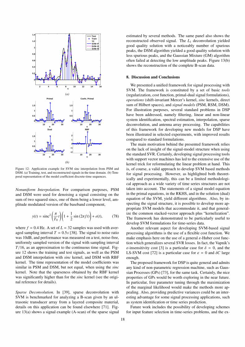
2 4 6 8 10 12 14 16
0
0.2
0.4
0.6
0.8
1
1.2
1.4
n
TestTrainY2SVM−PSVM−DSVM−R
(a)
10 20 30
0
0.5
1
1.5
n
Primal
10 20 30
0
0.5
1
1.5
n
Coefs. Primal
10 20 30
0
0.5
1
1.5
n
Dual
10 20 30−2
−1
0
1
2
n
RBF
(b)
Figure 12: Application example for SVM sinc interpolation from PSM andDSM. (a) Training, test, and reconstructed signals in the time domain. (b) Tem-poral representation of the model coefficient discrete-time sequences.
Nonuniform Interpolation. For comparison purposes, PSMand DSM were used for denoising a signal consisting on thesum of two squared sincs, one of them being a lower level, am-plitude modulated version of the baseband component,
y(t) = sinc2(π
T0t) (
1 +12
sin (2π f t))
+ e(t), (78)
where f = 0.4 Hz. A set of L = 32 samples was used with aver-aged sampling interval T = 0.5s [38]. The signal to noise ratiowas 10dB, and performance was measured on a test, noise-free,uniformly sampled version of the signal with sampling intervalT/16, as an approximation to the continuous time signal. Fig-ure 12 shows the training and test signals, as well as the PSMand DSM interpolation with sinc kernel, and DSM with RBFkernel. The time representation of the model coefficients wassimilar in PSM and DSM, but not equal, when using the sinckernel. Note that the sparseness obtained by the RBF kernelwas significantly higher than for the sinc kernel (see the origi-nal reference for details).
Sparse Deconvolution. In [39], sparse deconvolution withSVM is benchmarked for analyzing a B-scan given by an ul-trasonic transducer array from a layered composite material,details on this application can be found elsewhere [71]. Fig-ure 13(a) shows a signal example (A-scan) of the sparse signal
estimated by several methods. The same panel also shows thereconstructed observed signal. The L1 deconvolution yieldedgood quality solution with a noticeably number of spuriouspeaks, the DSM algorithm yielded a good quality solution withless spurious peaks, and the Gaussian Mixture (GM) algorithmoften failed at detecting the low amplitude peaks. Figure 13(b)shows the reconstruction of the complete B-scan data.
8. Discussion and Conclusions
We presented a unified framework for signal processing withSVM. The framework is constituted by a set of basic tools(regularization, cost function, primal-dual signal formulations),operations (shift-invariant Mercer’s kernel, sinc kernels, directsum of Hilbert spaces), and signal models (PSM, RSM, DSM).For illustration purposes, several standard problems in DSPhave been addressed, namely filtering, linear and non-linearsystem identification, spectral estimation, interpolation, sparsedeconvolution, and antenna array processing. The capabilitiesof this framework for developing new models for DSP havebeen illustrated in selected experiments, with improved resultscompared to standard formulations.
The main motivation behind the presented framework relieson the lack of insight of the signal-model structure when usingthe standard SVR. Certainly, developing signal processing toolswith support vector machines has led to the extensive use of thekernel trick for reformulating the linear problem at hand. Thisis, of course, a valid approach to develop SVM based methodsfor signal processing. However, as highlighted both theoret-ically and experimentally, this can be a limited methodologi-cal approach as a wide variety of time series structures are nottaken into account. The statements of a signal model equationin the primal equations, in the RKHS, and in the solution (dual)equation of the SVM, yield different algorithms. Also, by in-specting the signal structure, it is possible to develop more ap-propriate SVM models that accommodate it, and that general-ize the common stacked-vector approach plus “kernelization”.The framework has demonstrated to be particularly useful todevelop SVM formulations for time-series data.
Another relevant aspect for developing SVM-based signalprocessing algorithms is the use of a flexible cost function. Wemake emphasis here on the use of a general ε-Huber cost func-tion which generalizes several SVR losses. In fact, the Vapnik’sε-insensitivity cost [3] is a particular case for δ = 0, and theLS-SVM cost [72] is a particular case for ε = 0 and δC largeenough.
The proposed framework for DSP is quite general and admitsany kind of non-parametric regression machine, such as Gaus-sian Processes (GPs) [73], for the same task. Certainly, the niceproperties of GPs would be worth exploring in the near future.In particular, free parameter tuning through the maximizationof the marginal likelihood would make the methods more ap-pealing. Also, providing predictive variances could be an inter-esting advantage for some signal processing applications, suchas system identification or time series prediction.
Future work includes the possibility of developing schemesfor input feature selection in time-series problems, and the ex-
18
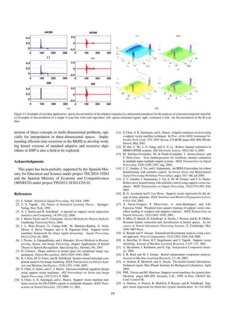
100 200 300
0
0.2
0.4
AKSM
0 100 200 300−0.5
0
0.5
AKSM
0
100 200 300
0
0.2
0.4
L1
0 100 200 300−0.5
0
0.5
L1
0
100 200 300
0
0.2
0.4
GM
0 100 200 300−0.5
0
0.5
GM
0
(a) (b)
Figure 13: Example of real data application: sparse deconvolution of the impulse response in a ultrasound transducer for the analysis of a layered composite material.(a) Example of deconvolution of a single A-scan line with each algorithm: left, sparse estimated signal; right, estimated A-line. (b) Deconvolution of the B-scandata.
tension of these concepts to multi-dimensional problems, spe-cially for interpolation in three-dimensional spaces. Imple-menting efficient time recursion in the RKHS to develop work-ing kernel versions of standard adaptive and recursive algo-rithms in DSP is also a field to be explored.
Acknowledgments
This paper has been partially supported by the Spanish Min-istry for Education and Science under project TEC2010-19263and the Spanish Ministry of Economy and Competitiveness(MINECO) under project TIN2012-38102-C03-01.
References
[1] L. Scharf. Statistical Signal Processing. NJ, USA, 1990.[2] V. N. Vapnik. The Nature of Statistical Learning Theory. Springer–
Verlag, New York, 1995.[3] A. J. Smola and B. Schölkopf. A tutorial on support vector regression.
Statistics and Computing, 14:199–222, 2004.[4] J. Shawe-Taylor and N. Cristianini. Kernel Methods for Pattern Analysis.
Cambridge University Press, 2004.[5] J. L. Rojo-Álvarez, G. Camps-Valls, M. Martínez-Ramón, E. Soria-
Olivas, A. Navia Vázquez, and A. R. Figueiras-Vidal. Support vectormachines framework for linear signal processing. Signal Processing,85(12):2316–26, 2005.
[6] J. Picone, A. Ganapathiraju, and J. Hamaker. Kernel Methods in Bioengi-neering, Signal, and Image Processing, chapter Applications of KernelTheory to Speech Recognition. Idea Group Inc., Hershey, PA, 2007.
[7] D. Cremers. Shape statistics in kernel space for variational image seg-mentation. Pattern Recognition, 36(9):1929–1943, 2003.
[8] K. I. Kim, M. O. Franz, and B. Schölkopf. Iterative kernel principal com-ponent analysis for image modeling. IEEE Transactions on Pattern Anal-ysis and Machine Intelligence, 27(9):1351–1366, 2005.
[9] S. Chen, S. Gunn, and C. J. Harris. Decision feedback equaliser designusing support vector machines. IEE Proceedings on Vision and ImageSignal Processing, 147(3):213–9, 2000.
[10] S. Chen, A. K. Samingan, and L. Hanzo. Support vector machine mul-tiuser receiver for DS-CDMA signals in multipath channels. IEEE Trans-actions on Neural Networks, 12(3):604–11, 2001.
[11] S. Chen, A. K. Sanmigan, and L. Hanzo. Adaptive mutiuser receiver usinga support vector machine technique. In Proc. of the IEEE Semianual Ve-hicular Tech. Conf., VTC 2001 Spring, CD-ROM, pages 604–608, Rhode,Greece, May 2001.
[12] W. Bai, C. He, L. G. Jiang, and X. X. Li. Robust channel estimation inMIMO-OFDM systems. IEE Electronic Letters, 39(2):242–4, 2003.
[13] M. Sánchez-Fernández, M. de Prado-Cumplido, J. Arenas-García, andF. Pérez-Cruz. Svm multiregression for nonlinear channel estimationin multiple-input multiple-output systems. IEEE Transactions on SignalProcessing, 52(8):2298–2307, aug. 2004.
[14] C. C. Gaudes, J. Via, and I. Santamaría. An IRWLS procedure for robustbeamforming with sidelobe control. In Sensor Array and MultichannelSignal Processing Workshop Proceedings, pages 342–346, jul 2004.
[15] C. C. Gaudes, I. Santamaria, J. Via, E. M. M. Gomez, and T. S. Paules.Robust array beamforming with sidelobe control using support vector ma-chines. IEEE Transactions on Signal Processing, 55(2):574–584, Feb.2007.
[16] R. G. Ayestaran and F. Las-Heras. Support vector regression for the de-sign of array antennas. IEEE Antennas and Wireless Propagation Letters,4:414–416, 2005.
[17] A. Navia-Vázquez, F. Pérez-Cruz, A. Artés-Rodríguez, and A.R.Figueiras-Vidal. Weighted least squares training of support vector clas-sifiers leading to compact and adaptive schemes. IEEE Transactions onNeural Networks, 12(5):1047–1059, 2001.
[18] S. Mika, G. Rätsch, B. Schölkopf, A. Smola, J. Weston, and K.-R. Müller.Invariant feature extraction and classification in kernel spaces. In Ad-vances in Neural Information Processing Systems 12, Cambridge, MA,1999. MIT Press.
[19] G. Baudat and F. Anouar. Generalized discriminant analysis using a ker-nel approach. Neural Computation, 12(2):2385–2404, Feb 2000.
[20] A. Ben-Hur, D. Horn, H.T. Siegelmann, and V. Vapnik. Support vectorclustering. Journal of Machine Learning Research, 2:125–137, 2001.
[21] A. Hyvärinen, J. Karhunen, and E. Oja. Independent Component Analy-sis. 2001.
[22] F. R. Bach and M. I. Jordan. Kernel independent component analysis.Journal of Machine Learning Research, 3:1–48, 2002.
[23] A. Gretton, R. Herbrich, and A. Smola. The kernel mutual information.Technical report, Max Planck Institute for Biological Cybernetics, April2003.
[24] PML. Drezet and RF. Harrison. Support vector machines for system iden-tification. pages 688–692, Swansea, U.K., 1998. in Proc. UKACC Int.Conf. Control’98.
[25] A. Gretton, A. Doucet, R. Herbrich, P. Rayner, and B. Schölkopf. Sup-port vector regression for black-box system identification. In 11th IEEE
19

Workshop on Statistical Signal Processing, pages 341–344. IEEE SignalProcessing Society, Piscataway, NY, Aug 2001.
[26] J. A. K. Suykens. Support Vector Machines: a nonlinear modelling andcontrol perspective. European Journal of Control, Special Issue on fun-damental issues in control, 7(2-3):311–327, 2001.
[27] J. A. K. Suykens, J. Vandewalle, and B. De Moor. Optimal control byleast squares support vector machines. Neural Networks, 14(1):23 – 35,2001.
[28] D. Mattera. Support Vector Machines for Signal Processing, pages 321–342. Studies in Fuzziness and Soft Computing. Springer, Berlin / Heidel-berg, 2005.
[29] I. Goethals, K. Pelckmans, J. A. K. Suykens, and B. De Moor. Subspaceidentification of Hammerstein systems using least squares support vectormachines. IEEE Transactions on Automatic Control, 50(10):1509–19,2005.
[30] M. A. Aizerman, E. M. Braverman, and L.I. Rozoner. Theoretical foun-dations of the potential function method in pattern recognition learning.Automation and remote Control, 25:821–837, 1964.
[31] J. L. Rojo-Álvarez, M. Martínez-Ramón, A. R. Figueiras-Vidal,A. García-Armada, and A. Artés-Rodríguez. A robust support vector al-gorithm for non-parametric spectral analysis. IEEE Signal ProcessingLetters, 10(11):320 – 323, Nov 2003.
[32] G. Camps-Valls, M. Martínez-Ramón, J.L. Rojo-Álvarez, and E. Soria-Olivas. Robust γ-filter using support vector machines. Neurocomputing,62:493–499, 2004.
[33] J. L. Rojo-Álvarez, M. Martínez-Ramón, M. dePrado Cumplido,A. Artés-Rodríguez, and A. R. Figueiras-Vidal. Support vector methodfor robust ARMA system identification. IEEE Transactions on SignalProcessing, 52(1):155 – 164, Jan 2004.
[34] M. Martínez-Ramón, Nan Xu, and C.G. Christodoulou. Beamformingusing support vector machines. IEEE Antennas and Wireless PropagationLetters, 4:439–442, 2005.
[35] A. El Gonnouni, M. Martinez-Ramon, J.L. Rojo-Alvarez, G. Camps-Valls, A.R. Figueiras-Vidal, and C.G. Christodoulou. A support vectormachine music algorithm. Antennas and Propagation, IEEE Transactionson, 60(10):4901–4910, 2012.
[36] M. Martínez-Ramón, J.L. Rojo-Álvarez, G. Camps-Valls, A. Navia-Vázquez, J. Muñoz-Marí, E. Soria-Olivas, and A.R. Figueiras-Vidal. Sup-port vector machines for nonlinear kernel arma system identification.IEEE Transactions on Neural Networks, 17:1617–1622, Nov. 2006.
[37] M. Martínez-Ramón, J.L. Rojo-Álvarez, G. Camps-Valls, and C.G.Christodoulou. Kernel antenna array processing. IEEE Transactions onAntennas and Propagation, 55(3):642–650, March 2007.
[38] J.L. Rojo-Ávarez, C.. Figuera-Pozuelo, C.E. Martinez-Cruz, G.. Camps-Valls, F.. Alonso-Atienza, and M.. Martinez-Ramon. Nonuniform inter-polation of noisy signals using support vector machines. IEEE Transac-tions on Signal Processing, 55(8):4116 –4126, aug. 2007.
[39] J. L. Rojo-Álvarez, , M. Martínez-Ramón, J. Muñoz-Marí, G. Camps-Valls, C. E. M. Cruz, and A. R. Figueiras-Vidal. Sparse deconvolutionusing support vector machines. EURASIP Journal on Advances in SignalProcessing, 2008.
[40] Carlos Figuera, José Luis Rojo-Álvarez, Mark Wilby, Inmaculada Mora-Jiménez, and Antonio J. Caamaño. Advanced support vector machinesfor 802.11 indoor location. Signal Processing, 9:2126–2136, 2012.
[41] Carlos Figuera, Óscar Barquero-Pérez, José Luis Rojo-Álvarez, ManelMartínez-Ramón, Alicia Guerrero-Curieses, and Antonio J. Caama no.Spectrally adapted Mercer kernels for support vector nonuniform inter-polation. Signal Processing, (in press)(-):–, 2013.
[42] J. Arenas-Garcia, K. Petersen, G. Camps-Valls, and L.K. Hansen. Kernelmultivariate analysis framework for supervised subspace learning: A tu-torial on linear and kernel multivariate methods. IEEE Signal ProcessingMagazine, 30(4):16–29, 2013.
[43] F. Pérez-Cruz, S. Van Vaerenbergh, J.J. Murillo-Fuentes, M. Lázaro-Gredilla, and I. Santamaría. Gaussian processes for nonlinear signal pro-cessing: An overview of recent advances. IEEE Signal Processing Mag-azine, 30(4):40–50, 2013.
[44] G. Ding, Q. Wu, Y.-D. Yao, J. Wang, and Y. Chen. Kernel-based learningfor statistical signal processing in cognitive radio networks: Theoreticalfoundations, example applications, and future directions. IEEE SignalProcessing Magazine, 30(4):126–136, 2013.
[45] N. Cristianini and J. Shawe-Taylor. Bayesian voting schemes and large
margin classifiers. In B. Schölkopf, C. J. C. Burges, and A. J. Smola,editors, Advances in Kernel Methods — Support Vector Learning, pages55–68, Cambridge, MA, 1999. MIT Press.
[46] V. Vapnik. Statistical Learning Theory, Adaptive and Learning Systemsfor Signal Processing, Communications, and Control. John Wiley &Sons, 1998.
[47] B. Schölkopf and A. Smola. Learning with Kernels. MIT Press, Cam-bridge, MA, 1st edition, 2002.
[48] J. Suykens, J. Vandewalle, and B. De Moor. Intelligence and cooperativesearch by coupled local minimizers. International Journal of Bifurcationand Chaos, 11(8):2133–2144, 2001.
[49] J. L. Rojo-Álvarez, M. Martínez-Ramón, A. R. Figueiras-Vidal, M. de-Prado Cumplido, and A. Artés-Rodríguez. Support Vector Method forARMA system identification: a robust cost interpretation. In Inter-national Conference on Artificial Neural Networks, ICANN2002. LNCS2415, Madrid, Spain., Aug 2002. Springer–Verlag.
[50] G. Camps-Valls., J. L. Rojo-Álvarez, and M. Martínez-Ramón, editors.Kernel Methods in Bioengineering, Signal, and Image Processing. IdeaGroup Inc., Hershey, PA, 2007.
[51] A. N. Tikhonov and V. Y. Arsenen. Solution to Ill-Posed Problems. V. H.Winston & Sons, 1977.
[52] S.L. Marple. Digital Spectral Analysis with Applications. Prentice-Hall,Englewood Cliffs, NJ, 1987.
[53] N. R. Lomb. Least-squares frequency analysis of unequally spaced data.Astrophysics and Space Science, 39:447–462, Feb 1976.
[54] L. Ljung. System Identification. Theory for the user. Prentice Hall, UpperSaddle River, N.J., 2nd edition, 1999.
[55] A.V. Oppenheim and R.W. Schafer. Discrete-time Signal Processing.Prentice Hall, Englewood Cliffs, New Jersey, 1989.
[56] J. L. Yen. On nonuniform sampling of bandwidth-limited signals. IRETransactions on Circuits Theory, 3(4):251–57, 1956.
[57] H. Choi and D. C. Munson Jr. Analysis and design of minimax-optimal in-terpolators. IEEE Transactions on Signal Processing, 46:1571–79, 1998.
[58] L. Ying and D. C. Munson. Approximation of the minmax interpolator. InProc. Int. Conf. on Acoust., Speech, and Signal Processing, ICASSP2000,volume 3, pages 328–331, Turkey, Jun 2000.
[59] I. Santamaría-Caballero, C.J. Pantaleón-Prieto, and A. Artés-Rodríguez.Sparse deconvolution using adaptive mixed-gaussian models. Signal Pro-cessing, 54:161–172, 1996.
[60] S. A. Kassam and H. V. Poor. Robust techniques for signal processing: Asurvey. Proceedings IEEE, 73:433–482, 1985.
[61] H. Van Trees. Detection, Estimation, and Modulation Theory. John Wiley& Sons, New York, 2002.
[62] L. Zhang, Z. Weida, and L. Jiao. Wavelet support vector machine. IEEETransactions on Systems, Man, and Cybernetics B, 34(1):34–39, Feb.2004.
[63] T. Söderström and P. Stoica. System Identification. Prentice-Hall, Engle-wood Cliffs, NJ, US, 1987.
[64] A. Gretton, M. Davy, A. Doucet, and P. J. W. Rayner. Nonstationary sig-nal classification using support vector machines. In 11th IEEE Workshopon Statistical Signal Processing, pages 305–308, Piscataway, NY, 2001.IEEE Signal Processing Society.
[65] M. Espinoza, J. A. K. Suykens, and B. De Moor. Kernel based partiallylinear models and nonlinear identification. IEEE Transactions on Auto-matic Control, 50(10):1602–6, 2005.
[66] O. Nelles. Nonlinear System Identification. From classical approaches toNeural Networks and Fuzzy Models. Springer-Verlag, Berlin HeidelbergNew York, 2001.
[67] G. Camps-Valls, M. Martínez-Ramón, J. L. Rojo-Álvarez, and J. Muñoz-Marí. Non-linear system identification with composite relevance vectormachines. IEEE Signal Processing Letters, 14(4):279–282, April 2007.
[68] G. Camps-Valls, J. Muñoz-Marí, M. Martínez-Ramón, J. Requena-Carrión, and J.L. Rojo-Álvarez. Learning non-linear time-scales withkernel γ-filters. Neurocomputing, 72:1324–1328, 2008.
[69] A. Papoulis. Probability Random Variables and Stochastic Processes.McGraw-Hill, New York, USA, 3 edition, 1991.
[70] B. Schölkopf, A. Smola, and K. R. Müller. Nonlinear component analy-sis as a kernel eigenvalue problem. Neural Computation, 10:1299–1319,1998.
[71] T. Olofsson. Semi-sparse deconvolution robust to uncertainties in theimpulse responses. Ultrasonics, 42:969–975, 2004.
20

[72] J. A. K. Suykens and J. Vandewalle. Recurrent least squares support vec-tor machines. IEEE Transactions on Circuits and Systems-I, 47(7):1109–1114, 2000.
[73] C. E. Rasmussen and C. K. I. Williams. Gaussian Processes for MachineLearning. The MIT Press, Cambridge, MA, 2006.
References
[1] L. Scharf. Statistical Signal Processing. NJ, USA, 1990.[2] V. N. Vapnik. The Nature of Statistical Learning Theory. Springer–
Verlag, New York, 1995.[3] A. J. Smola and B. Schölkopf. A tutorial on support vector regression.
Statistics and Computing, 14:199–222, 2004.[4] J. Shawe-Taylor and N. Cristianini. Kernel Methods for Pattern Analysis.
Cambridge University Press, 2004.[5] J. L. Rojo-Álvarez, G. Camps-Valls, M. Martínez-Ramón, E. Soria-
Olivas, A. Navia Vázquez, and A. R. Figueiras-Vidal. Support vectormachines framework for linear signal processing. Signal Processing,85(12):2316–26, 2005.
[6] J. Picone, A. Ganapathiraju, and J. Hamaker. Kernel Methods in Bioengi-neering, Signal, and Image Processing, chapter Applications of KernelTheory to Speech Recognition. Idea Group Inc., Hershey, PA, 2007.
[7] D. Cremers. Shape statistics in kernel space for variational image seg-mentation. Pattern Recognition, 36(9):1929–1943, 2003.
[8] K. I. Kim, M. O. Franz, and B. Schölkopf. Iterative kernel principal com-ponent analysis for image modeling. IEEE Transactions on Pattern Anal-ysis and Machine Intelligence, 27(9):1351–1366, 2005.
[9] S. Chen, S. Gunn, and C. J. Harris. Decision feedback equaliser designusing support vector machines. IEE Proceedings on Vision and ImageSignal Processing, 147(3):213–9, 2000.
[10] S. Chen, A. K. Samingan, and L. Hanzo. Support vector machine mul-tiuser receiver for DS-CDMA signals in multipath channels. IEEE Trans-actions on Neural Networks, 12(3):604–11, 2001.
[11] S. Chen, A. K. Sanmigan, and L. Hanzo. Adaptive mutiuser receiver usinga support vector machine technique. In Proc. of the IEEE Semianual Ve-hicular Tech. Conf., VTC 2001 Spring, CD-ROM, pages 604–608, Rhode,Greece, May 2001.
[12] W. Bai, C. He, L. G. Jiang, and X. X. Li. Robust channel estimation inMIMO-OFDM systems. IEE Electronic Letters, 39(2):242–4, 2003.
[13] M. Sánchez-Fernández, M. de Prado-Cumplido, J. Arenas-García, andF. Pérez-Cruz. Svm multiregression for nonlinear channel estimationin multiple-input multiple-output systems. IEEE Transactions on SignalProcessing, 52(8):2298–2307, aug. 2004.
[14] C. C. Gaudes, J. Via, and I. Santamaría. An IRWLS procedure for robustbeamforming with sidelobe control. In Sensor Array and MultichannelSignal Processing Workshop Proceedings, pages 342–346, jul 2004.
[15] C. C. Gaudes, I. Santamaria, J. Via, E. M. M. Gomez, and T. S. Paules.Robust array beamforming with sidelobe control using support vector ma-chines. IEEE Transactions on Signal Processing, 55(2):574–584, Feb.2007.
[16] R. G. Ayestaran and F. Las-Heras. Support vector regression for the de-sign of array antennas. IEEE Antennas and Wireless Propagation Letters,4:414–416, 2005.
[17] A. Navia-Vázquez, F. Pérez-Cruz, A. Artés-Rodríguez, and A.R.Figueiras-Vidal. Weighted least squares training of support vector clas-sifiers leading to compact and adaptive schemes. IEEE Transactions onNeural Networks, 12(5):1047–1059, 2001.
[18] S. Mika, G. Rätsch, B. Schölkopf, A. Smola, J. Weston, and K.-R. Müller.Invariant feature extraction and classification in kernel spaces. In Ad-vances in Neural Information Processing Systems 12, Cambridge, MA,1999. MIT Press.
[19] G. Baudat and F. Anouar. Generalized discriminant analysis using a ker-nel approach. Neural Computation, 12(2):2385–2404, Feb 2000.
[20] A. Ben-Hur, D. Horn, H.T. Siegelmann, and V. Vapnik. Support vectorclustering. Journal of Machine Learning Research, 2:125–137, 2001.
[21] A. Hyvärinen, J. Karhunen, and E. Oja. Independent Component Analy-sis. 2001.
[22] F. R. Bach and M. I. Jordan. Kernel independent component analysis.Journal of Machine Learning Research, 3:1–48, 2002.
[23] A. Gretton, R. Herbrich, and A. Smola. The kernel mutual information.Technical report, Max Planck Institute for Biological Cybernetics, April2003.
[24] PML. Drezet and RF. Harrison. Support vector machines for system iden-tification. pages 688–692, Swansea, U.K., 1998. in Proc. UKACC Int.Conf. Control’98.
[25] A. Gretton, A. Doucet, R. Herbrich, P. Rayner, and B. Schölkopf. Sup-port vector regression for black-box system identification. In 11th IEEEWorkshop on Statistical Signal Processing, pages 341–344. IEEE SignalProcessing Society, Piscataway, NY, Aug 2001.
[26] J. A. K. Suykens. Support Vector Machines: a nonlinear modelling andcontrol perspective. European Journal of Control, Special Issue on fun-damental issues in control, 7(2-3):311–327, 2001.
[27] J. A. K. Suykens, J. Vandewalle, and B. De Moor. Optimal control byleast squares support vector machines. Neural Networks, 14(1):23 – 35,2001.
[28] D. Mattera. Support Vector Machines for Signal Processing, pages 321–342. Studies in Fuzziness and Soft Computing. Springer, Berlin / Heidel-berg, 2005.
[29] I. Goethals, K. Pelckmans, J. A. K. Suykens, and B. De Moor. Subspaceidentification of Hammerstein systems using least squares support vectormachines. IEEE Transactions on Automatic Control, 50(10):1509–19,2005.
[30] M. A. Aizerman, E. M. Braverman, and L.I. Rozoner. Theoretical foun-dations of the potential function method in pattern recognition learning.Automation and remote Control, 25:821–837, 1964.
[31] J. L. Rojo-Álvarez, M. Martínez-Ramón, A. R. Figueiras-Vidal,A. García-Armada, and A. Artés-Rodríguez. A robust support vector al-gorithm for non-parametric spectral analysis. IEEE Signal ProcessingLetters, 10(11):320 – 323, Nov 2003.
[32] G. Camps-Valls, M. Martínez-Ramón, J.L. Rojo-Álvarez, and E. Soria-Olivas. Robust γ-filter using support vector machines. Neurocomputing,62:493–499, 2004.
[33] J. L. Rojo-Álvarez, M. Martínez-Ramón, M. dePrado Cumplido,A. Artés-Rodríguez, and A. R. Figueiras-Vidal. Support vector methodfor robust ARMA system identification. IEEE Transactions on SignalProcessing, 52(1):155 – 164, Jan 2004.
[34] M. Martínez-Ramón, Nan Xu, and C.G. Christodoulou. Beamformingusing support vector machines. IEEE Antennas and Wireless PropagationLetters, 4:439–442, 2005.
[35] A. El Gonnouni, M. Martinez-Ramon, J.L. Rojo-Alvarez, G. Camps-Valls, A.R. Figueiras-Vidal, and C.G. Christodoulou. A support vectormachine music algorithm. Antennas and Propagation, IEEE Transactionson, 60(10):4901–4910, 2012.
[36] M. Martínez-Ramón, J.L. Rojo-Álvarez, G. Camps-Valls, A. Navia-Vázquez, J. Muñoz-Marí, E. Soria-Olivas, and A.R. Figueiras-Vidal. Sup-port vector machines for nonlinear kernel arma system identification.IEEE Transactions on Neural Networks, 17:1617–1622, Nov. 2006.
[37] M. Martínez-Ramón, J.L. Rojo-Álvarez, G. Camps-Valls, and C.G.Christodoulou. Kernel antenna array processing. IEEE Transactions onAntennas and Propagation, 55(3):642–650, March 2007.
[38] J.L. Rojo-Ávarez, C.. Figuera-Pozuelo, C.E. Martinez-Cruz, G.. Camps-Valls, F.. Alonso-Atienza, and M.. Martinez-Ramon. Nonuniform inter-polation of noisy signals using support vector machines. IEEE Transac-tions on Signal Processing, 55(8):4116 –4126, aug. 2007.
[39] J. L. Rojo-Álvarez, , M. Martínez-Ramón, J. Muñoz-Marí, G. Camps-Valls, C. E. M. Cruz, and A. R. Figueiras-Vidal. Sparse deconvolutionusing support vector machines. EURASIP Journal on Advances in SignalProcessing, 2008.
[40] Carlos Figuera, José Luis Rojo-Álvarez, Mark Wilby, Inmaculada Mora-Jiménez, and Antonio J. Caamaño. Advanced support vector machinesfor 802.11 indoor location. Signal Processing, 9:2126–2136, 2012.
[41] Carlos Figuera, Óscar Barquero-Pérez, José Luis Rojo-Álvarez, ManelMartínez-Ramón, Alicia Guerrero-Curieses, and Antonio J. Caama no.Spectrally adapted Mercer kernels for support vector nonuniform inter-polation. Signal Processing, (in press)(-):–, 2013.
[42] J. Arenas-Garcia, K. Petersen, G. Camps-Valls, and L.K. Hansen. Kernelmultivariate analysis framework for supervised subspace learning: A tu-torial on linear and kernel multivariate methods. IEEE Signal ProcessingMagazine, 30(4):16–29, 2013.
[43] F. Pérez-Cruz, S. Van Vaerenbergh, J.J. Murillo-Fuentes, M. Lázaro-
21
Gredilla, and I. Santamaría. Gaussian processes for nonlinear signal pro-cessing: An overview of recent advances. IEEE Signal Processing Mag-azine, 30(4):40–50, 2013.
[44] G. Ding, Q. Wu, Y.-D. Yao, J. Wang, and Y. Chen. Kernel-based learningfor statistical signal processing in cognitive radio networks: Theoreticalfoundations, example applications, and future directions. IEEE SignalProcessing Magazine, 30(4):126–136, 2013.
[45] N. Cristianini and J. Shawe-Taylor. Bayesian voting schemes and largemargin classifiers. In B. Schölkopf, C. J. C. Burges, and A. J. Smola,editors, Advances in Kernel Methods — Support Vector Learning, pages55–68, Cambridge, MA, 1999. MIT Press.
[46] V. Vapnik. Statistical Learning Theory, Adaptive and Learning Systemsfor Signal Processing, Communications, and Control. John Wiley &Sons, 1998.
[47] B. Schölkopf and A. Smola. Learning with Kernels. MIT Press, Cam-bridge, MA, 1st edition, 2002.
[48] J. Suykens, J. Vandewalle, and B. De Moor. Intelligence and cooperativesearch by coupled local minimizers. International Journal of Bifurcationand Chaos, 11(8):2133–2144, 2001.
[49] J. L. Rojo-Álvarez, M. Martínez-Ramón, A. R. Figueiras-Vidal, M. de-Prado Cumplido, and A. Artés-Rodríguez. Support Vector Method forARMA system identification: a robust cost interpretation. In Inter-national Conference on Artificial Neural Networks, ICANN2002. LNCS2415, Madrid, Spain., Aug 2002. Springer–Verlag.
[50] G. Camps-Valls., J. L. Rojo-Álvarez, and M. Martínez-Ramón, editors.Kernel Methods in Bioengineering, Signal, and Image Processing. IdeaGroup Inc., Hershey, PA, 2007.
[51] A. N. Tikhonov and V. Y. Arsenen. Solution to Ill-Posed Problems. V. H.Winston & Sons, 1977.
[52] S.L. Marple. Digital Spectral Analysis with Applications. Prentice-Hall,Englewood Cliffs, NJ, 1987.
[53] N. R. Lomb. Least-squares frequency analysis of unequally spaced data.Astrophysics and Space Science, 39:447–462, Feb 1976.
[54] L. Ljung. System Identification. Theory for the user. Prentice Hall, UpperSaddle River, N.J., 2nd edition, 1999.
[55] A.V. Oppenheim and R.W. Schafer. Discrete-time Signal Processing.Prentice Hall, Englewood Cliffs, New Jersey, 1989.
[56] J. L. Yen. On nonuniform sampling of bandwidth-limited signals. IRETransactions on Circuits Theory, 3(4):251–57, 1956.
[57] H. Choi and D. C. Munson Jr. Analysis and design of minimax-optimal in-terpolators. IEEE Transactions on Signal Processing, 46:1571–79, 1998.
[58] L. Ying and D. C. Munson. Approximation of the minmax interpolator. InProc. Int. Conf. on Acoust., Speech, and Signal Processing, ICASSP2000,volume 3, pages 328–331, Turkey, Jun 2000.
[59] I. Santamaría-Caballero, C.J. Pantaleón-Prieto, and A. Artés-Rodríguez.Sparse deconvolution using adaptive mixed-gaussian models. Signal Pro-cessing, 54:161–172, 1996.
[60] S. A. Kassam and H. V. Poor. Robust techniques for signal processing: Asurvey. Proceedings IEEE, 73:433–482, 1985.
[61] H. Van Trees. Detection, Estimation, and Modulation Theory. John Wiley& Sons, New York, 2002.
[62] L. Zhang, Z. Weida, and L. Jiao. Wavelet support vector machine. IEEETransactions on Systems, Man, and Cybernetics B, 34(1):34–39, Feb.2004.
[63] T. Söderström and P. Stoica. System Identification. Prentice-Hall, Engle-wood Cliffs, NJ, US, 1987.
[64] A. Gretton, M. Davy, A. Doucet, and P. J. W. Rayner. Nonstationary sig-nal classification using support vector machines. In 11th IEEE Workshopon Statistical Signal Processing, pages 305–308, Piscataway, NY, 2001.IEEE Signal Processing Society.
[65] M. Espinoza, J. A. K. Suykens, and B. De Moor. Kernel based partiallylinear models and nonlinear identification. IEEE Transactions on Auto-matic Control, 50(10):1602–6, 2005.
[66] O. Nelles. Nonlinear System Identification. From classical approaches toNeural Networks and Fuzzy Models. Springer-Verlag, Berlin HeidelbergNew York, 2001.
[67] G. Camps-Valls, M. Martínez-Ramón, J. L. Rojo-Álvarez, and J. Muñoz-Marí. Non-linear system identification with composite relevance vectormachines. IEEE Signal Processing Letters, 14(4):279–282, April 2007.
[68] G. Camps-Valls, J. Muñoz-Marí, M. Martínez-Ramón, J. Requena-Carrión, and J.L. Rojo-Álvarez. Learning non-linear time-scales with
kernel γ-filters. Neurocomputing, 72:1324–1328, 2008.[69] A. Papoulis. Probability Random Variables and Stochastic Processes.
McGraw-Hill, New York, USA, 3 edition, 1991.[70] B. Schölkopf, A. Smola, and K. R. Müller. Nonlinear component analy-
sis as a kernel eigenvalue problem. Neural Computation, 10:1299–1319,1998.
[71] T. Olofsson. Semi-sparse deconvolution robust to uncertainties in theimpulse responses. Ultrasonics, 42:969–975, 2004.
[72] J. A. K. Suykens and J. Vandewalle. Recurrent least squares support vec-tor machines. IEEE Transactions on Circuits and Systems-I, 47(7):1109–1114, 2000.
[73] C. E. Rasmussen and C. K. I. Williams. Gaussian Processes for MachineLearning. The MIT Press, Cambridge, MA, 2006.
22