a unified approach for handling convection terms in finite...
TRANSCRIPT

IMA Journal of Numerical AnalysisPage 1 of 45doi:10.1093/imanum/drq018
A unified approach for handling convection terms in finite volumesand mimetic discretization methods for elliptic problems
BEIRAO DA VEIGA
Dipartimentodi Matematica ‘F. Enriques’, Universita degli Studi di Milano, via Saldini 50,20133 Milano, Italy
JEROME DRONIOU∗
Institut de Mathematiques et de Modelisation de Montpellier, Universite Montpellier 2,CC 051, Place Eugene Bataillon, 34095 Montpellier cedex 5, France
∗Correspondingauthor. Email: [email protected]
GIANMARCO MANZINI
Istitutodi Matematica Applicata e Tecnologie Informatiche—CNR, via Ferrata 1,27100 Pavia, Italy
[Received on 24 September 2009; revised on 27 April 2010]
We study the numerical approximation to the solution of the steady convection–diffusion equation. Thediffusion term is discretized by using the hybrid mimetic method (HMM), which is the unified formula-tion for the hybrid finite-volume (FV) method, the mixed FV method and the mimetic finite-differencemethod recently proposed inDroniou et al. (2010, Math. Models Methods Appl. Sci., 20, 265–295).In such a setting we discuss several techniques to discretize the convection term that are mainly adaptedfrom the literature on FV or FV schemes. For this family of schemes we provide a full proof of conver-gence under very general regularity conditions of the solution field and derive an error estimate whenthe scalar solution is inH2(Ω). Finally, we compare the performance of these schemes on a set of testcases selected from the literature in order to document the accuracy of the numerical approximation inboth diffusion- and convection-dominated regimes. Moreover, we numerically investigate the behaviourof these methods in the approximation of solutions with boundary layers or internal regions with stronggradients.
Keywords: finite-volume methods; mimetic finite-difference methods; convection-diffusion equation;convection-dominated flows; convergence analysis; error estimates.
1. Introduction
Many physical models of fluid flows involve partial differential equations (PDEs) with both convectionand diffusion terms, such as the Navier–Stokes equations, flows in porous media, etc. Analytical so-lutions are not normally available for real applications and numerical approximations must be devisedin some way. For this purpose efficient numerical schemes based on finite and mixed finite elementand two-point finite volumes (FVs) have been developed for the numerical treatment of the diffusivepart of the equation. In such a framework a great amount of work has been done to investigate the
c© Theauthor 2010. Published by Oxford University Press on behalf of the Institute of Mathematics and its Applications. All rights reserved.
IMA Journal of Numerical Analysis Advance Access published December 15, 2010 at U
niversite D'A
ix-Marseille on N
ovember 19, 2014
http://imajna.oxfordjournals.org/
Dow
nloaded from

2 of 45 B. DA VEIGA ET AL.
connectionsbetween the lowest order Raviart–Thomas mixed finite-element (RT0 − P0) methods andvarious cell-centred FV and finite-difference numerical formulations on meshes of simplexes and quadri-laterals/hexahedrons. The relationship between the mixed finite-element method and the cell-centredfinite-difference method on rectangular meshes was first established inRussell & Wheeler(1983) andfurther developed in subsequent papers (see, for example,Arbogastet al., 1998). Basically, it can beshown that, by applying appropriate quadrature rules to the numerical formulation in theRT0 spaceon rectangles, the vector variable (the velocity) is eliminated, thus reducing the method to a positive-definite cell-centred finite-difference method for the scalar variable (the pressure). Using this approach,classical cell-centred finite-difference methods on rectangular meshes are easily retrieved based on anine-point stencil for full tensor coefficients and a five-point stencil for a scalar (diagonal) tensor. Simi-lar results are also obtainable on regular hexahedral meshes. These developments led to the formulationof enhanced cell-centred finite differences (cf.Arbogastet al.,1998) that can handle general shape el-ements (triangles, quadrilaterals and hexahedra) and are suitable for full tensor coefficients. A similarrelationship exists between theRT0−P0 schemeand the two-point FV formulation on triangular meshesusing triangle circumcentres. This relationship was originally established byBarangeret al. (1996) fortwo-dimensional diffusion problems with scalar coefficients. This approach has been further developedin Youneset al.(2004), which investigates the case of a full diffusion tensor in two and three dimensionson meshes of simplexes.
Nonetheless, practical situations, such as those encountered in petroleum engineering, require com-putational grids that are not structured or simple enough to make use of the methods mentioned above.Thus, alternative and more sophisticated techniques have been developed in the last decade to approx-imate the solution to diffusive equations on general grids. In this framework we mention, for instance,the discontinuous Galerkin method (Arnold et al., 2002; Riviere, 2008, and references therein), themulti-point flux approximation (Aavatsmarket al., 1998a,b;Wheeler & Yotov, 2006), the mimeticfinite-difference (MFD) method (Berndtet al.,2001;Hymanet al.,2002;Brezziet al.,2005a,b,2007,2009;Kuznetsovet al.,2005;Beirao da Veiga, 2008;Beirao da Veiga & Manzini,2008a,b;Cangiani &Manzini,2008;Beirao da Veigaet al.,2009b;Lipnikov et al.,2009, and references therein), the hybridFV method (Eymardet al., 2009) and the mixed FV method (Droniou & Eymard,2006; Chainais-Hillairet & Droniou, 2007;Droniou & Eymard,2009). Strict correlations also exist among these nu-merical approximations and with respect to the lowest order mixed finite-element method, and it is notsurprising that sometimes the lowest order schemes may belong to more than one of these families ofmethods. For example, the first-order discontinuous Galerkin scheme can be easily reinterpreted as anFV method. The lowest order Raviart–Thomas scheme on grids of simplexes (triangles in two dimen-sions and tetrahedrons in three dimensions) is a member of the family of MFD methods (cf.Cangiani& Manzini, 2008). Note, however, that on meshes of quadrilaterals and hexahedrons no connection hasyet been established between the MFD method in mixed form and the mixed finite-element method. Wealso mention the paper byVohralik (2006) that outlined the relationship existing between the multi-pointflux approximation and the mixed finite-element method.
A remarkable fact has been recently discovered inDroniou et al. (2010), which showed that aftersome generalization, a unified formulation exists for three of the methods cited above, namely, thehybrid FV method, the mixed FV method and the MFD method. Consequently, these three methods aremembers of the same family of discretization techniques. FollowingDroniouet al.(2010), we will referto such a family of numerical methods ashybrid mimetic mixedmethods or use the abbreviation HMM.
Since the HMM method can be considered as the meeting of two different frameworks, namely,the mimetic/finite-element and the FV ones, the convective term can be naturally discretized using quitedifferent techniques depending on the adopted point of view on the scheme. There are, indeed, two
at Universite D
'Aix-M
arseille on Novem
ber 19, 2014http://im
ajna.oxfordjournals.org/D
ownloaded from

A UNIFIED APPROACH FOR HANDLING CONVECTION TERMS 3 of 45
possible approaches: either the diffusive flux is approximated, and then some form of centred or upwindapproximation of the convection term is considered in the discretization of the divergence equation, orthe total flux, which includes both diffusive and convective terms, is approximated, which leads to acentred-type approximation of the convection terms. The first approach is, perhaps, more popular in thefinite-difference and FV practitioner community (cf.Chainais-Hillairet & Droniou, 2009;Droniou &Eymard,2009), while the second approach seems to be more popular in the finite-element practitionercommunity. Nevertheless, it is worth mentioning that both approaches have been considered in theframework of mixed finite-element methods (seeDouglas & Roberts,1982,1985;Jaffre & Roberts,1985).
In the MFD setting a numerical discretization of the full diffusion and convection fluxes has beenproposed byCangianiet al. (2009). A proper reformulation of the mimetic scheme as a conformingmethod, using the finite-dimensional subspace ofH(div,Ω) given by the lifting of the degrees of free-dom of the vector variable, makes it possible to perform the convergence analysis in a very similar wayto that presented inDouglas & Roberts(1985).
From this overview we can conclude that several numerical discretizations of the convection–diffusion equations that may fit in the HMM setting have been proposed in the literature. However, nosystematic study has been carried out so far on the possible ways, and related advantages and drawbacks,in which a convective term can be treated numerically by using the more general HMM formulation. Itis our main goal in this work to perform such an investigation in order to assess the behaviour of suchmethods both theoretically and numerically.
The plan of the paper is as follows. In Section2 we recall the principles of the HMM schemes forthe pure diffusion equation, and we discuss how to discretize the convection term, using some centred,upwind or exponential fitting-like choice in accordance with a two-point FV flux formula (or, from thepoint of view of finite elements, seeJaffre(1984) andDawson & Aizinger(1999)). We also show thatthe numerical approximation proposed inCangianiet al.(2009), possibly with a stabilization term, is anHMM method to which the theoretical analysis of the present paper applies. In Section3 we provide fullproofs of convergence under very general regularity conditions when the mesh size tends to zero andderive error estimates in suitable mesh-dependent norms when the scalar solution is inH2(Ω). Section4is devoted to the presentation and discussion of how various instances of the HMM discretizationsperform when applied to a set of standard test cases for the convection–diffusion equations, includingthe approximation of solutions with boundary and internal layers. Finally, conclusions are given inSection5.
2. The HMM formulation for convection–diffusion problems
2.1 The mathematical model
Let us consider the steady convection–diffusion equation
−div(Λ∇ p) + div(V p) = f in Ω, (2.1)
p = gD on ∂Ω (2.2)
under the following hypotheses:
(H1) Ω is a bounded, open, polygonal subset ofRd with d > 1;
(H2) Λ : Ω → Md(R) is a bounded, measurable, symmetric and uniformly elliptic tensor;
at Universite D
'Aix-M
arseille on Novem
ber 19, 2014http://im
ajna.oxfordjournals.org/D
ownloaded from

4 of 45 B. DA VEIGA ET AL.
(H3) f ∈ L2(Ω);
(H4) V ∈ C1(Ω)d is such that div(V) > 0.
Moreover, let us introduce the diffusive flux and the total flux as follows:
F = −Λ∇ p and F = F + V p. (2.3)
For simplicity, we will restrict the presentation of a the methods and the theoretical analysis to the caseof a homogeneous Dirichlet boundary condition by settinggD = 0 in (2.2) and we will consider thenonhomogeneous case in the numerical experiments of Section4.
Under assumptions (H1)–(H4), the existence and uniqueness of a weak solution inH10 (Ω) to (2.1)
and (2.2) with gD = 0 is completely standard since the bilinear form associated with this problem iscontinuous and coercive.
REMARK 2.1 TheC1 regularity assumption onV in (H4) can be weakened for the convergence study(see Section3.1.3). We assume the smoothness of the convection field in order to simplify a little bitsome (already lengthy) technical arguments and also to prove error estimates.
2.2 Mesh notation and regularity
Let us begin with the definition of an admissible discretization ofΩ and the related notation.
DEFINITION 2.2 (Admissible discretization). An admissible discretization ofΩ is given by the tripletDh = (Ωh, Eh,Ph), where themesh size hwill be defined in the following and where the followingconditions hold.
• HereΩh is a finite family of nonempty open polygonal disjoint subsetsE of Ω, the cells of themesh, suchthatΩ =
⋃E∈Ωh
E.
• HereEh is a finite family of nonempty open disjoint subsetse of Ω, thefacesof the mesh, such that,for all e ∈ Eh, there exists an affine hyperplaneA of Rd anda cellE ∈ Ωh suchthate ⊂ (E\E)∩A.We also assume that the following hold:
- for all E ∈ Ωh thereexists a subset∂E of Eh suchthat E\E =⋃
e∈∂E e;
- for all e ∈ Eh eitherwe have thate ⊂ ∂Ω or we have thate ⊂ E ∩ E′ for some pair of elementsE, E′ ∈ Ωh with E 6= E′.
• HerePh is a family of points ofΩ indexed byE, that is,Ph = (xE)E∈Ωh , and such that each meshcell E is star shaped with respect toxE.
REMARK 2.3 When all of the mesh cells are convex shaped a convenient choice for the points(xE)E∈Ωh
is given, for instance, by the centre of gravity of the cells.
The d-dimensional measure of each cellE is denoted by|E| and the cell size byhE. As usual,the mesh size is given byh = supE∈Ωh
hE. For consistency of notation,|e| andhe denotethe (d −1)-dimensional measure of facee and the face diameter. For each facee ∈ Eh we let xe denotethebarycentre ofe andne
E its normal direction pointing out ofE. Moreover, with each facee we associatethe unit normal vectorne, whose orientation is arbitrarily chosen whene is an internal face, and assumedto be pointing out ofΩ whene is a boundary face. We denote the set of the internal faces byEh,int, thatis, Eh,int = {e ∈ Eh for e 6⊂ ∂Ω}, and the set of the boundary faces byEh,ext, that is,Eh,ext = {e ∈
at Universite D
'Aix-M
arseille on Novem
ber 19, 2014http://im
ajna.oxfordjournals.org/D
ownloaded from

A UNIFIED APPROACH FOR HANDLING CONVECTION TERMS 5 of 45
Eh for e ⊂ ∂Ω}. We will find it convenient to denote the two cells that share an internal facee by Eand E′ and, where required, to fix the orientation ofe so thatne
E ∙ ne = 1. Finally, we introduce thefollowing geometric quantities that will be useful in the definition of the numerical convection flux inSection2.4.1:
dE,e is the= distance betweenxE and the hyperplane containinge
and
de =
{dE,e + dE′,e for any internal facee ∈ Eh,int,
dE,e for any boundary facee ∈ Eh,ext.
Figure1 illustrates some of this notation.The proof of convergence forh → 0 that we present in Section3 requires the following very mild
geometrical assumptions on the meshes ofDh.
(G1) Every mesh cellE is star shaped with respect to the corresponding pointxE.
(G2) For any internal facee ∈ Eh,int let us introduceMe = {E, E′}, that is, the cells on the oppositeside ofe. Then the quantity
regul(Dh) = max
(max
e∈Eh,int,(E,E′)∈Me
dE,e
dE′,e, max
E∈Ωh,e∈∂E
hE
dE,e, max
E∈ΩhCard(∂E)
),
which expresses the mesh regularity, isuniformlybounded from above forh → 0.
In the mimetic framework a similar condition is often used, and we state this as follows.
(ME) [Star-shaped elements] There exists a positive numberτ ∗ such that each elementE is star shapedwith respect toall the points of a ball of radiusτ ∗hE centred atxE.
Stronger conditions on the mesh regularity are required to derive an error estimate for the HMM ap-proximations to the exact solution and flux. We formulate these mesh regularity conditions ford = 3.The restriction to other dimensions is straightforward.
FIG. 1. Mesh notation.
at Universite D
'Aix-M
arseille on Novem
ber 19, 2014http://im
ajna.oxfordjournals.org/D
ownloaded from
6 of 45 B. DA VEIGA ET AL.
(HG) [Shape regularity] There exist two positive real numbersNs andρs, independent ofh, such thatevery meshΩh of the sequence admits a subpartition into tetrahedronsSh suchthat we have thefollowing.
(HG1) The decomposition of every polyhedronE ∈ Ωh, denoted bySh|E, is formed by at mostNs tetrahedrons,and each vertex ofΩh is a vertex ofSh.
(HG2) Every tetrahedron ofSh is shaperegular in the sense that the ratio betweenrT , the radiusof its inscribed sphere, andhT , its diameter, is bounded from below byρs. Formally, wehave that
∀ T ∈ Sh :rT
hT> ρs > 0.
Fromthe above assumptions, several properties of the mesh that are useful in the error analysis of themimetic formulation can be derived. For the sake of the reader’s convenience, we list them below forfuture reference in the paper.
(M1) There exist two positive integersNE and Ne that are independent ofh, E ∈ Ωh ande ∈ Eh
andsuch that every elementE has Card(∂E) 6 NE faces, and every facee has Card(∂e) 6 Ne
edges.
(M2) For any mesh elementE ∈ Ωh the quantities|E|, |e| for e ∈ ∂E and|l| for each edgel ∈ ∂eproperly scale with respect tohE. In particular, there exists a positive constanta∗ suchthat
a∗hd−1E 6 |e|, a∗hE 6 he, a∗hd−2
E 6 |l|.
(M3) There exists a constantCAg thatis independent ofhE andsuch that (Brezziet al.,2005a)∑
e∈∂E
||φ||2L2(e) 6 CAg(h−1E ||φ||2L2(E)
+ hE|φ|2H1(E)) (2.4)
for any functionφ ∈ H1(E). We will refer to (2.4) as theAgmon inequality.
(M4) For any functionq ∈ H2(E) thereexists alinear polynomialL1(q) interpolatingq anda constantC, independent ofhE, such that (Brenner & Scott,1994)
||q − L1(q)||L2(E)+hE|q − L1(q)|H1(E)6Ch2E|q|H2(E). (2.5)
2.3 Discretization of the diffusion term
To approximate (2.1) and (2.2) we introduce the space of thediscrete scalar fields Qh andthe space ofthediscrete flux fields Xh. The discrete scalarsq ∈ Qh aredefined by taking one degree of freedom percell, denoted byqE, that is,q = (qE)E∈Ωh . Therefore the spaceQh canbe identified with the space ofthe piecewise constant polynomials defined onΩh. Similarly, thediscrete fluxesare defined by takingone degree of freedom per face per element, denoted byFe
E, that is,F = (FeE)e∈∂E
E∈Ωh, which represents
the normal flux across the facee in the directionneE. We require that every fluxF ∈ Xh satisfiesthe
following flux conservation propertyat any internal face:
∀ e ∈ Eh,int, e ⊂ ∂E ∪ ∂E′ : FeE + Fe
E′ = 0, (2.6)
sothat the elements ofXh only possess one degree of freedom per face, and the sign ofFeE dependson
the orientation of the facee with respect toE. The restriction of theF to the cellE ∈ Ωh is denoted byFE = (Fe
E)e∈∂E andrepresents the collection of the normal fluxes in the directionsneE for e ∈ ∂E. The
at Universite D
'Aix-M
arseille on Novem
ber 19, 2014http://im
ajna.oxfordjournals.org/D
ownloaded from

A UNIFIED APPROACH FOR HANDLING CONVECTION TERMS 7 of 45
set of these vector fields forms the linear spaceXE. Throughout the paper we will also make use of thesymbol Xh to denote the linear space of thediscontinuous fluxes, that is, of the vectors having the sameform F = (Fe
E)e∈∂EE∈Ωh
but that do not satisfy condition (2.6). Note thatXh is a linear subspace ofXh.
Thenext ingredient of the HMM formulation is thediscrete divergence operatordivh : Xh → Qh,which is defined as follows:
∀ G ∈ Xh, ∀E ∈ Ωh : (divh(G))E =1
|E|
∑
e∈∂E
|e|GeE. (2.7)
With any sufficiently regular vector fieldG and scalar fieldq we associate the interpolated fieldsGI ∈ Xh andqI ∈ Qh thatare given by
∀ e ∈ Eh : (GI )e =1
|e|
∫
eG ∙ ne and ∀ E ∈ Ωh : (qI )E =
1
|E|
∫
Eq. (2.8)
REMARK 2.4 The definition of the discrete divergence operator in (2.7) is consistent with the Gaussdivergence theorem for the interpolations of (2.8), so that the following commutation property holds:
(div(G))I = divh(GI ). (2.9)
We endowQh with the usualL2(Ω) scalar product for piecewise constant functions, that is,[∙, ∙]Qh := [∙, ∙]L2. On the other hand,Xh and Xh areequipped with the scalar product
[F, G] Xh=
∑
E∈Ωh
[FE, GE]E (2.10)
thatassembles the locally defined scalar products [∙, ∙]E. The local scalar products([∙, ∙]E) satisfythefollowing coercivity and consistency assumptions.
(S1) There exist two positive constantsσ∗ andσ ∗, independent of the mesh sizeh, such that, for everymesh cellE, we have
σ∗|E|∑
e∈∂E
(GeE)2 6 [G, G]E 6 σ ∗|E|
∑
e∈∂E
(GeE)2 ∀ G ∈ Xh .
(S2) For every elementE we have that
[(ΛE∇q1)I , G]E = −[divh(G), q1]L2(E) +∑
e∈∂E
GeE
∫
eq1
for all G ∈ Xh andall linear polynomialsq1, whereΛE is the cell average ofΛ.
REMARK 2.5 HereΛE is actually an approximation ofΛ|E, the restriction of the diffusion tensorΛ tothe cellE. To prove the convergence of the numerical solution in Section3.1, we only require that thediffusion tensorΛ satisfy the regularity assumption (H2), while we need a stronger regularity conditionto derive the error estimates of Section3.2. In this latter case we will find it convenient to assume (H2)and also thatΛ be locally Lipschitz continuous onΩh, that is, for allE ∈ Ωh, the components ofΛ|EareLipschitz continuous functions onE. Consequently,ΛE canbe any constant approximation ofΛ|Esuchthat the estimate
maxi, j =1,d
supx∈E
|(ΛE)i j − Λi j (x)| = O(h)
holds.
at Universite D
'Aix-M
arseille on Novem
ber 19, 2014http://im
ajna.oxfordjournals.org/D
ownloaded from

8 of 45 B. DA VEIGA ET AL.
The construction of a family of scalar products satisfying the above assumptions whenxE is thecentre of gravity ofE can be found inBrezzi et al. (2005b). Moreover, in this case it was provedin Droniouet al. (2010) that (S1) and (S2) lead necessarily to the following form:
∀(FE, GE) ∈ XE : [FE, GE]E = |E|ΛEvE(FE) ∙ vE(GE) + TE(GE)TBETE(FE), (2.11)
where
vE(FE) = −1
|E|Λ−1
E
∑
e∈∂E
|e|FeE(xe − xE) (2.12)
is a constant approximation of∇ p on the cellE, TE(FE) = (TE,e(Fe))e∈∂E is given by
TE,e(FE) = FeE + ΛEvE(FE) ∙ ne
E, (2.13)
andBE is a symmetric positive-definite matrix of size Card(∂E). More precisely, it turns out that thematrixBE satisfiesthe following coercivity condition that is directly related to (S1).
(C) There exists a positive constantα, that is independent of the mesh size such that, for allE ∈ Ωh
andGE ∈ XE, we have that
α∑
e∈∂E
|e|dE,e(TE,e(GE))2 6 TE(GE)TBETE(GE) 61
α
∑
e∈∂E
|e|dE,e(TE,e(GE))2.
If xE is not the barycentre ofE, then the same construction (2.11)–(2.13) still holds provided that (S2)is modified by introducing a suitable integration weight (seeDroniouet al.,2010).
The HMM discretization of problem (2.1) and (2.2) withV = 0, which provides us with the desiredapproximation of the diffusion operator, takes the following form:
find (ph, Fh) ∈ Qh × Xh suchthat
∀ G ∈ Xh : [Fh, G] Xh= [divh(G), ph]Qh, (2.14)
∀ q ∈ Qh : [divh(Fh), q]Qh = [ f, q]Qh . (2.15)
Here ph ∈ Qh andFh ∈ Xh arethe approximations topI andF I , the interpolations of the exact scalarsolution p and its fluxF = −Λ∇ p.
The HMM method can be easily hybridized through the introduction ofH(Eh), the space of facevaluesqEh = (qe)e∈Eh ∈ RCard(Eh) with qe = 0 for e ∈ Eh,ext, and imposing explicitly the flux conserva-tion property (2.6). The discrete variational form (2.14) and (2.15) with [∙, ∙]E satisfying(2.11)–(2.13)is equivalent to the following:
find (ph, Fh, pEh) ∈ Qh × Xh × H(Eh) suchthat
∀ E ∈ Ωh, ∀ GE ∈ XE : [FE, GE]E =∑
e∈∂E
|e|GeE(pE − pe), (2.16)
∀ E ∈ Ωh :∑
e∈∂E
|e|FeE =
∫
Ef, (2.17)
∀ e ∈ Eh,int, : FeE + Fe
E′ = 0, (2.18)
at Universite D
'Aix-M
arseille on Novem
ber 19, 2014http://im
ajna.oxfordjournals.org/D
ownloaded from

A UNIFIED APPROACH FOR HANDLING CONVECTION TERMS 9 of 45
whereE, E′ ∈ Ωh arethe two elements such thate ⊂ ∂E ∩ ∂E′ for everye ∈ Eh,int. Under suitableassumptions on the regularity of the exact solutionp, the additional unknownspEh = (pe)e∈Eh approxi-matethe face average of the exact solution over each mesh face. We will formalize this concept throughthe introduction ofpJ ∈ H(Eh), the face interpolation ofp, in Section3.2(see equation (3.43)).
2.4 Discretization of the convective term
As discussed in Section 1, two different strategies can be considered for the numerical treatment of theconvection term in the HMM discretization of an elliptic problem. In the first strategy, which is reviewedin Section2.4.1, we introduce some form of centred or upwind approximation of the convection termin the discretization of the divergence equation provided by the HMM method (cf.Chainais-Hillairet &Droniou,2009;Droniou & Eymard,2009). In the second strategy, which is reviewed in Section2.4.2,the total flux, which includes both diffusive and convective terms, is approximated, thus leading to acentred-type approximation of the convection terms (cf.Cangianiet al., 2009). Both approaches wereconsidered for the mixed finite-element method inDouglas & Roberts(1982,1985) andJaffre & Roberts(1985). It turns out that, in the new framework of HMM methods, a unified formulation is possible,which is the topic of Section2.4.3. We end this section with a discussion on an alternative hybridizedform of the numerical convection terms (Section2.4.4).
In the rest of this section we assume that the velocity fieldV is a continuous function with a contin-uous derivative, that is,V ∈ C1(Ω)d. The cell restriction of its interpolation inXh is given by the set ofreal numbers(Ve
E)e∈∂E ∈ XE suchthat
∀e ∈ ∂E : VeE =
1
|e|
∫
eV ∙ ne
E. (2.19)
2.4.1 FV-baseddiscretizations. Several discretization schemes for the convection term are availablein the FV literature, for example, the second-order centred scheme, the first-order upwind scheme, theθ -scheme, the Scharfetter–Gummel scheme, etc. In these methods, the convection flux of the exact solutionfield p is approximated through the numerical convection flux of the discrete scalar fieldph ∈ Qh. Thisnumerical convection flux is given by the collection of real numbersFc(ph) = (Fc(ph)e
E)E∈Ωh,e∈∂E
suchthat
∀ E ∈ Ωh, ∀ e ∈ ∂E :1
|e|
∫
eVp ∙ ne
E ≈ (Fc(ph))eE. (2.20)
We list below the schemes that we will explicitly consider in the section on numerical experiments. Welet E′ bethe cell on the other side ofe if e ∈ Eh,int andassume for notational simplicity thatpE′ = 0 ife ∈ Eh,ext.
• Thesecond-order centered schemeis given by the approximation
1
|e|
∫
eVp ∙ ne
E ≈ (Fc(ph))eE = Ve
EpE + pE′
2.
• Thefirst-order upwind schemeis given by the approximation
1
|e|
∫
eVp ∙ ne
E ≈ (Fc(ph))eE = (Ve
E)+ pE − (VeE)− pE′ ,
with s± = max(±s, 0).
at Universite D
'Aix-M
arseille on Novem
ber 19, 2014http://im
ajna.oxfordjournals.org/D
ownloaded from

10of 45 B. DA VEIGA ET AL.
• Theθ -schemeis given by the approximation
1
|e|
∫
eVp ∙ ne
E ≈ (Fc(ph))eE = (Ve
E)+((1 − θ)pE + θpE′) − (VeE)−((1 − θ)pE′ + θpE)
= (1 − 2θ)((VeE)+ pE − (Ve
E)− pE′) + θVeE(pE + pE′),
with θ ∈ [0, 1/2]. This choice is clearly intermediate between the centred and the upwind schemes.
• TheScharfetter–Gummel scheme(Scharfetter & Gummel,1969) is given by the approximation
1
|e|
∫
eVp ∙ ne
E ≈ (Fc(ph))eE =
1
de(Asg(deVe
E)pE − Asg(−deVeE)pE′), (2.21)
with
Asg(s) =−s
e−s − 1− 1. (2.22)
Note that the first three approaches above can also be found in the finite-element literature (see, forinstance,Jaffre(1984) andDawson & Aizinger(1999)). As pointed out inChainais-Hillairet & Droniou(2009), the Scharfetter–Gummel scheme inScharfetter & Gummel(1969) was written for an isotropichomogeneous material, that is,Λ = I . In the original formulation, diffusion and convection terms weresimultaneously treated to define the numerical flux. Removing the diffusive part in the numerical fluxformulation allows us to obtain the formulas (2.21) and (2.22). This definition of a pure convectiveflux through the simple elimination of the diffusive part is somewhat basic in the general caseΛ 6=I , especially if some eigenvalues ofΛ are small. Although the above definition ofAsg ensurestheL2-stability of the scheme, it can give quite bad solutions in convection-dominated cases. This factcan be understood if one comes back to the two-point FV scheme for−εΔp + div(V p) = f . Thenthe choice (2.22) ensures the maximum principle of the scheme only ifε > 1, while the maximumprinciple is lost numerically ifε < 1. When applying the Scharfetter–Gummel method to compute thenumerical convective flux, a better choice is provided by locally scalingAsg in accordance with thesmallest eigenvalue ofΛ. If e is the face betweenE andE′ andλe is the smallest eigenvalue ofΛE andΛE′ , then we use
Asg,Λ,e(s) = min(1,λe)Asg
(s
min(1,λe)
)(2.23)
insteadof Asg(s) in (2.21). In this way the numerical flux automatically and locally adjusts the upwind-ing of the convection term depending on its strength with respect to the diffusive term without perturbingthe consistency property ofAsg. Note thatλe → 0 implies thatλeAsg(s/λe) → s+. Therefore, if thelocal diffusion is very small, then this implementation of the Scharfetter–Gummel method allows theflux to adjust to upwinding automatically, thus bringing enough numerical diffusion to ensure a betterstability.Once an FV-based discretization of the convective term has been chosen, the divergence of the convec-tion term in (2.1), that is, div(V p), is approximated onE by
(div(V p))IE ≈
1
|E|
∑
e∈∂E
|e|(Fc(ph))eE = divh(Fc(ph))|E
at Universite D
'Aix-M
arseille on Novem
ber 19, 2014http://im
ajna.oxfordjournals.org/D
ownloaded from

A UNIFIED APPROACH FOR HANDLING CONVECTION TERMS 11of 45
and the HMM approximation to the model problem (2.1) and (2.2) then reads as follows:find (ph, Fh) ∈ Qh × Xh suchthat
∀ G ∈ Xh : [Fh, G] Xh= [divh(G), ph]Qh, (2.24)
∀ q ∈ Qh : [divh(Fh + Fc(ph)), q]Qh = [ f I , q]Qh . (2.25)
2.4.2 MFD-baseddiscretizations. From a theoretical standpoint, MFDs have only very recently ap-proached problems that are different to the pure diffusion one (see, for instance,Beirao da Veigaet al.,2009a,2010;Beirao da Veiga,2010). To our knowledge, the only paper considering the development anderror analysis of convection–diffusion equations directly in the framework of MFD is that ofCangianiet al. (2009). In this subsection we briefly review the formulation and the major convergence results ofthe method considered in that paper, and we show how it can be reformulated as an HMM method.
Let H(div,Ω) be the space of vector fields all of whose components are square integrable functionsand that have square integrable divergence. Formally,
H(div,Ω) = {v ∈ (L2(Ω))d suchthat div(v) ∈ L2(Ω)}
is a Hilbert space when equipped with the scalar product
[v, u]H(div,Ω) =∫
Ωv ∙ u +
∫
Ωdiv(v) div(u)
and the corresponding norm
||v||2H(div,Ω) = ||v||2L2(Ω)+ ||div(v)||2L2(Ω)
.
In Cangianietal. (2009) a numerical approximation was considered to themixed variational formulationof problem (2.1) and (2.2), which reads as follows (Brezzi & Fortin,1991):
find (F, p) ∈ (div,Ω) × L2(Ω) such that
∀ v ∈ H(div,Ω) : [Λ−1F, v]L2 − [ p, div(v)]L2 − [Λ−1Vp, v]L2 = 0, (2.26)
∀ q ∈ L2(Ω) : [div(F), q]L2 = [ f, q]L2, (2.27)
whereF is the total vector flux defined in (2.3).To discretize the convection term we transform the corresponding variational term as follows:
∀ v ∈ H(div,Ω) : [Λ−1Vp, v]L2 ≈∑
E∈Ωh
∫
EΛ−1
E Vp ∙ v −→ ∀ G ∈ Xh :∑
E∈Ωh
pE[V I , G]E,
wherethe components of the interpolated velocity fieldV I ∈ Xh, that is,(V I )eE for all E ∈ Ωh and
e ∈ ∂E, are given by (2.19), and the local scalar products are required to satisfy assumptions (S1) and(S2). The mimetic variational formulation presented inCangianiet al. (2009) reads as follows:
find (Fh, ph) ∈ Xh × Qh suchthat
∀G ∈ Xh : [ Fh, G] Xh− [ ph, divh(G)]Qh −
∑
E∈Ωh
pE[V I , G]E = 0, (2.28)
∀q ∈ Qh : [divh(Fh), q]Qh = [ f I , q]Qh . (2.29)
at Universite D
'Aix-M
arseille on Novem
ber 19, 2014http://im
ajna.oxfordjournals.org/D
ownloaded from

12of 45 B. DA VEIGA ET AL.
Theconvergence analysis of this scheme was carried out inCangianiet al. (2009) under assumptionson the grid regularity that are substantially equivalent to (HG) and (ME). When the scalar solutionp isin H2(Ω) the analysis provides the following error estimate:
|||Fh − F I |||Xh+ |||ph − pI |||Qh 6 Ch||p||H2(Ω), (2.30)
where ||| ∙ |||Xhand ||| ∙ |||Qh are the norms induced by the inner products of the spacesXh and Qh,
respectively. It is worth mentioning that the approximation of the scalar variable is superconvergentwhen the calculation is performed on a wide set of meshes. Superconvergence was also theoreticallyproved under some stronger assumptions on the regularity of the domain shape, the source term and thevelocity field.
Despite convergence being proved forh → 0 this scheme is expected to become unstable whenthe model problem is dominated by convection. This fact usually manifests through spurious effectslike numerical undershoots, overshoots or oscillations that may appear in the approximate solution. Toimprove stability we modify the divergence equation by introducing a stabilization term that dependson the solution’s jumps at mesh faces. We use the symbolsE andE′ to denote the two distinct cells thatshare the facee whene is internal and assume the orientation ofe to be such thatne
E ∙ ne = 1. Let usnow introduce thejumpof the discrete scalar fieldqh ∈ Qh asfollows:
[[qh]]e =
{qE − qE′ for e ∈ Eh,int,
qE for e ∈ Eh,ext.(2.31)
Equation(2.29) is substituted by
∀ q ∈ Qh : [divh(Fh) + Jh(ph), q]Qh = [ f I , q]Qh, (2.32)
wherethe stabilization termJh(ph) is given by
Jh(ph)|E =α
2|E|
∑
e∈∂E
|e||(V I )eE|[[ ph]]e, (2.33)
andα is a non-negative parameter that can be tuned to control the amount of numerical dissipation ofthe scheme.
This approach formally differs from the method introduced in Section 2.4.1 for FV-based discretiza-tions in that the convection term is numerically treated as part of the mimetic flux equation. However, itis possible to ‘extract’ an explicit form of the numerical convection flux from the scheme given by equa-tions (2.28) and (2.32) to reformulate it as an HMM method. For this purpose, we define the collectionof numbersFh = (Fe
E)E∈Ωh,e∈∂E by
FeE = Fe
E − pE(V I )eE. (2.34)
Equation(2.28) shows thatFh satisfies(2.14) and therefore plays the role of a purely diffusive flux.Moreover, noting that the stabilization termJh(ph) is locally written as a balance of fluxes, that is, adiscrete divergence, allows us to identify the convective flux as
(Fc(ph))eE = pE(V I )e
E +α
2|(V I )e
E|(pE − pE′) (2.35)
at Universite D
'Aix-M
arseille on Novem
ber 19, 2014http://im
ajna.oxfordjournals.org/D
ownloaded from

A UNIFIED APPROACH FOR HANDLING CONVECTION TERMS 13of 45
(we let pE′ = 0 if e is a boundary edge), so that (2.32) is simply given by divh(Fh + Fc(ph)) = f I .Thestabilized MFD scheme (2.28) and (2.32) can therefore be written as follows:
find ph ∈ Qh andFh ∈ Xh suchthat
∀ G ∈ Xh : [Fh, G] Xh= [divh(G), ph]Qh, (2.36)
∀ q ∈ Qh : [divh(Fh + Fc(ph)), q]Qh = [ f I , q]Qh, (2.37)
∀ e ∈ Eh,int : (Fh + (Fc(ph))eE + (Fh + (Fc(ph))
eE′ = 0. (2.38)
Notethat the diffusive fluxFh andthe convective fluxFc(ph) arenot conservative in the sense of (2.6)when considered separately and therefore belong to the linear spaceXh. However, their sum, that is,Fh + Fc(ph), is conservative since it belongs toXh in view of equation (2.38).
2.4.3 Unified setting. A unified formulation exists for the numerical discretization of the convec-tion term. This formulation includes the FV-based discretizations, as was noted inChainais-Hillairet &Droniou(2009), and the MFD-based discretization (2.36)–(2.38). This fact makes it possible to simplifythe software implementation and carry out a unified theoretical analysis.
Let us consider two functionsA, B : R → R and choose the numerical convection flux as thecollection of real numbers
Fc(ph) = (Fc(ph)eE)E∈Ωh,e∈∂E (2.39)
suchthat
∀ E ∈ Ωh, ∀ e ∈ ∂E : (Fc(ph))eE :=
1
de(A(deVe
E)pE + B(deVeE)pE′). (2.40)
Sincein the MFD discretization of the convection term these flux components are not conservative, thediffusive flux components cannot be conservative either and conservation must be imposed on the totalflux. The generic HMM approximation to the model problem (2.1) and (2.2) is thus written as follows:
find ph ∈ Qh andFh ∈ Xh suchthat
∀ G ∈ Xh : [Fh, G] Xh= [divh(G), ph]Qh, (2.41)
∀ q ∈ Qh : [divh(Fh + Fc(ph)), q]Qh = [ f I , q]Qh, (2.42)
∀ e ∈ Eh,int : (Fh + (Fc(ph))eE + (Fh + (Fc(ph))
eE′ = 0. (2.43)
Theschemes presented in Sections 2.4.1 and 2.4.2 can all be included in this general setting, withthe following choices ofA andB:
• centred scheme: A(s) = Ace(s) := s2 andB(s) = −Ace(−s) = s
2;
• upwindscheme:A(s) = Aup(s) := s+ andB(s) = −Aup(−s) = −s−;
• θ -scheme:A(s) = Aθ (s) := (1 − 2θ)Aup(s) + 2θAce(s) andB(s) = −Aθ (−s);
• Scharfetter–Gummel scheme: A(s) = Asg(s) definedby (2.22) andB(s) = −Asg(−s), and thelocally scaled Scharfetter–Gummel scheme is obtained by usingAsg,Λ,e definedby (2.23) instead ofAsg;
• stabilizedMFD scheme: A(s) = s + α2 |s| andB(s) = −α
2 |s|.
at Universite D
'Aix-M
arseille on Novem
ber 19, 2014http://im
ajna.oxfordjournals.org/D
ownloaded from

14of 45 B. DA VEIGA ET AL.
Thefirst four choices in (2.40) lead to a conservative definition of the numerical convection flux, whereasthe last one does not. However, in all of the cases mentioned above, total conservation is ensuredby (2.43). We note that all of these choices ofA andB satisfy the following properties:
(AB1) A : R → R andB : R → R are Lipschitz-continuous functions andA(0) = B(0) = 0;
(AB2) A(s) + B(s) = s for any real numbers;
(AB3) One of the following two alternatives holds:
(AB3-s) A(s) + B(−s) = 0 andA(s) − B(s) > 0 for any real numbers;
(AB3-w) the functions → A(s) + B(−s) is odd and there existsC > 0 such thatA(s) − B(s) >−C|s| for any real numbers.
We refer to (AB3-s) as thestrong (AB3) condition and to (AB3-w) as theweak (AB3) condition.Assumption (AB3-s) is satisfied by all of the FV-based discretizations listed above, whereas the MFD-based discretization satisfies (AB3-w). In fact, conditionA(s) + B(−s) = 0 in (AB3-s) is the oneensuring the conservation of the numerical convection flux (2.40). On the other hand, the numericalconvection flux extracted from the MFD-based formulation satisfies (AB3-w) and hence is not conser-vative. We will see in Section3 that assumptions (AB1)–(AB3) are enough to carry out the theoreticalanalysis of the scheme in (2.39)–(2.43), with slightly different results depending on which alternative in(AB3) is satisfied.
REMARK 2.6 It is worth noting that equation (2.42) can be rewritten in an FV form as the followingcell-based flux balance equation:
∀ E ∈ Ωh :∑
e∈∂E
|e|(FeE + (Fc(ph))e
E) =∫
Ef. (2.44)
REMARK 2.7 We could also choose, in (2.40), different functionsA = Ae and B = Be for eachedgee, provided that all these functions satisfy (AB1)–(AB3) and that their Lipschitz constants remainuniformly bounded as the mesh size tends to 0. This setting would allow the scheme to make a finertuning of the numerical diffusion due to upwinding, thus better adapting the scheme behaviour to thelocation inside the domain or the local geometry of the mesh.
2.4.4 An alternative hybrid discretization of the convection term.An alternative discretization of theconvection term is possible by using the hybridized valuepe in (2.40) instead ofpE′ , an idea introducedin Arnold & Brezzi (1985). In such a case we define the numerical convection flux of the discrete scalarfield described by(ph, pEh) ∈ Qh × H(Eh) asthe collection of real numbers
Fc,Eh(ph, pEh) = ((Fc,Eh(ph, pEh))eE)E∈Ωh,e∈∂E (2.45)
suchthat
∀ E ∈ Ωh, ∀ e ∈ ∂E : (Fc,Eh(ph, pEh))eE =
1
de(A(deVe
E)pE + B(deVeE)pe). (2.46)
Thesubstantial difference with the preceding choice (2.40) is that no property ofA andB ensures thatthe fluxesFc,Eh(ph, pEh) areconservative (and they are not in general). However, this will not bringany additional difficulty in the theoretical study provided that the following weaker form of (AB3) isconsidered.
at Universite D
'Aix-M
arseille on Novem
ber 19, 2014http://im
ajna.oxfordjournals.org/D
ownloaded from

A UNIFIED APPROACH FOR HANDLING CONVECTION TERMS 15of 45
(AB3h) One of the following strong or weak alternatives holds:
(AB3h-s) A(s) − B(s) > 0 for any real numbers;
(AB3h-w) there existsC > 0 such thatA(s) − B(s) > −C|s| for any real numbers.
The hybrid HMM formulation can then be written as follows:find (ph, Fh, pEh) ∈ Qh × Xh × H(Eh) suchthat
∀ E ∈ Ωh, ∀ GE ∈ XE : [FE, GE]E =∑
e∈∂E
|e|GeE(pE − pe), (2.47)
∀ E ∈ Ωh :∑
e∈∂E
|e|(FeE + (Fc,Eh(ph, pEh))
eE) =
∫
Ef, (2.48)
∀ e ∈ Eh,int : (Fh + (Fc,Eh(ph, pEh))eE + (Fh + (Fc,Eh(ph, pEh))
eE′ = 0, (2.49)
where the local scalar products used in (2.47) satisfy (S1) and (S2) and may thus be given in theform (2.11)–(2.13).
REMARK 2.8 An important advantage of discretizing the convective fluxes by using (2.45) and (2.46) in-stead of (2.39) and (2.40) is that the unknownsph andFh in the resulting numerical formulation (2.47)–(2.49) can be eliminated bystatic condensation, that is, through a local Gaussian elimination (thisclassical technique is not directly applicable to (2.39) and (2.40)). This procedure, which is commonfor hybrid mixed finite elements, provides a reduced linear system in the face unknownspEh . Moreover,when the discretization of the convection term increases significantly the numerical diffusion, as, forexample, in the case of the upwind scheme, the hybrid version of the HMM method is likely to be lessdiffusive than that provided by (2.39) and (2.40).
3. Theoretical study
In the present section we develop the theoretical analysis for the class of methods that we wish to investi-gate in this work. In Section3.1we prove the convergence of the numerical approximations to the exactsolution and its gradient. The analysis is based on a compactness argument, which is common in theFV literature, under the weaker assumptions of mesh regularity (G1) and (G2) (see also Definition2.2).In Section3.2 we prove anO(h) convergence rate for the numerical approximation of both the scalarsolution and the flux. The analysis involves stability and consistency arguments, which are in the MFD(and finite-element method) literature, under the stronger mesh regularity assumptions (HG) and (ME).
Let us introduce the mesh-dependent norms for the spacesXh and Qh. Let Dh be an admissiblemesh in accordance with Definition2.2 that satisfies (G1) and (G2) or, alternatively, (HG) and (ME).The scalar product inXh inducesthe norm
|||G|||2Xh
= [G, G] Xh∀ G ∈ Xh, (3.1)
andits local counterpart
|||G|||2E = [GE, GE]E ∀ GE ∈ XE. (3.2)
Theelements ofQh canbe identified with theΩh-piecewise constant functions and the scalar prod-uct in Qh is, in fact, theL2 scalarproduct for such functions. Therefore it is quite natural to consider
at Universite D
'Aix-M
arseille on Novem
ber 19, 2014http://im
ajna.oxfordjournals.org/D
ownloaded from

16of 45 B. DA VEIGA ET AL.
theL2 norm.However, we will also find it useful to carry out the analysis by using the discreteH10 -like
norm
||qh||1,Dh =
∑
E∈Ωh
∑
e∈∂E
|e|dE,e
(|qE − qE′ |
de
)2
1/2
∀ qh ∈ Qh, (3.3)
where E′ is the cell on the other side ofe ∈ ∂E ∩ Eh,int and, to ease notation, we takeqE′ = 0 ife ∈ ∂E ∩ Eh,ext. We will also need the following discreteH1 normon Qh × H(Eh):
||(qh, qEh)||1,Dh,Eh =
∑
E∈Ωh
∑
e∈∂E
|e|
dE,e|qE − qe|
2
1/2
∀(qh, qEh) ∈ Qh × H(Eh). (3.4)
It is easy to see that this norm is stronger than (3.3). More precisely, ifθ > regul(Dh), then there existsa constantC that is only dependent onθ such that, for all(qh, qEh) ∈ Qh × H(Eh), we have that
||qh||1,Dh 6 C||(qh, qEh)||1,Dh,Eh . (3.5)
In the following developments we will number all constants whose value may be zero depending onwhich alternative is considered in (AB3), that is, the strong (AB3-s) or the weak (AB3-w) condition.We will also use the symbol. to indicate an upper bound that holds up to a positive multiplicativeconstant that is independent ofh. However, we will trace explicitly the constants where required by theproofs or that may be zero depending on the choice of assumption (AB3).
LEMMA 3.1 Let us assume that (H1)–(H3) hold. LetDh bean admissible discretization ofΩ such thatθ > regul(Dh), and letFc(q) bethe convective flux ofq ∈ Qh given by (2.39) and (2.40) for the vectorfield V ∈ C1(Ω)d with A andB satisfyingassumptions (AB1)–(AB3). Then there exists a non-negativeconstantC1 > 0 that only depends onθ, V, A and Bsuch that
∀(q, qEh) ∈ Qh × H(Eh) :
1
2
∫
Ωq2div(V) 6
∑
E∈Ωh
∑
e∈∂E
|e|(Fc(q))eE(qE − qe) + C1h||(q, qEh)||
21,Dh,Eh
, (3.6)
andwhereC1 = 0 if (AB3-s) holds.
Proof. By gathering the sum by faces, we transform the term involvingFc(q) on the right-hand sideof (3.6) as follows:
∑
E∈Ωh
∑
e∈∂E
|e|(Fc(q))eE(qE − qe) =
∑
e∈Eh
|e|((Fc(q))eE(qE − qe) + (Fc(q))e
E′(qE′ − qe))
=∑
e∈Eh
|e|(Fc(q))eE(qE − qE′) (3.7)
+∑
e∈Eh
|e|((Fc(q))eE + (Fc(q))e
E′)(qE′ − qe).
at Universite D
'Aix-M
arseille on Novem
ber 19, 2014http://im
ajna.oxfordjournals.org/D
ownloaded from

A UNIFIED APPROACH FOR HANDLING CONVECTION TERMS 17of 45
To handle the first term on the right-hand side of (3.7) we note that, by using (2.40) and writing, due to(AB2),
A(deVeE) = 1
2(deVeE + A(deVe
E) − B(deVeE)),
B(deVeE) = 1
2(deVeE + B(deVe
E) − A(deVeE)),
(3.8)
wehave
(Fc(q))eE =
1
2Ve
E(qE + qE′) +1
2de(A(deVe
E) − B(deVeE))(qE − qE′).
Thereforewe infer that
∑
e∈Eh
|e|(Fc(q))eE(qE − qE′) =
1
2
∑
e∈Eh
|e|VeE(qE + qE′)(qE − qE′)
+1
2
∑
e∈Eh
|e|
de(A(deVe
E) − B(deVeE))(qE − qE′)2. (3.9)
Then,let us observe that∑
e∈Eh
|e|(qE − qE′)2 .∑
E∈Ωh
∑
e∈∂E
|e|(qE − qe)2 . h||(q, qEh)||
21,Dh,Eh
. (3.10)
By using (AB3), the conservation of(VeE)E∈Ωh,e∈∂E, the fact that
∑e∈∂E |e|Ve
E =∫
E div(V), andinequality (3.10), we obtain the following estimate:
∑
e∈Eh
|e|(Fc(q))eE(qE − qE′) >
1
2
∑
e∈Eh
|e|VeE(q2
E − q2E′) − C2
∑
e∈Eh
|e|(qE − qE′)2
>1
2
∑
E∈Ωh
q2E
∑
e∈∂E
|e|VeE − C3h||(q, qEh)||
21,Dh,Eh
>1
2
∫
Ωq2div(V) − C3h||(q, qEh)||
21,Dh,Eh
, (3.11)
whereC2 andC3 only depend onθ, V, A andB, andC2 = C3 = 0 if (AB3-s) holds.From (2.40) and sinceVe
E = −VeE′ , we have
(Fc(q))eE + (Fc(q))e
E′ =1
de([ A(deVe
E) + B(−deVeE)]qE + [B(deVe
E) + A(−deVeE)]qE′).
If (AB3-s) holds, then this quantity is equal to zero (this is the conservation of the convective flux), andif (AB3-w) holds, then we have, due to (AB1), that
|(Fc(q))eE + (Fc(q))e
E′ | =1
de|(A(deVe
E) + B(−deVeE))(qE − qE′)| 6 C4||V ||∞|qE − qE′ |
at Universite D
'Aix-M
arseille on Novem
ber 19, 2014http://im
ajna.oxfordjournals.org/D
ownloaded from

18of 45 B. DA VEIGA ET AL.
for someC4 thatis only dependent onA andB. Writing |qE − qE′ | 6 |qE − qe| + |qe − qE′ | andagainusing inequality (3.10) allows us to estimate the last term of (3.7) as follows:∣∣∣∣∣∣
∑
e∈Eh
|e|((Fc(q))eE + (Fc(q))e
E′)(qE′ − qe)
∣∣∣∣∣∣6 C5
∑
E∈Ωh
∑
e∈∂E
|e|(qE − qe)2 6 C5h||(q, qEh)||
21,Dh,Eh
,
(3.12)whereC5 only depends onV , A andB, and we have thatC5 = 0 if (AB3-s) holds.
The proof terminates by gathering inequalities (3.11) and (3.12) into (3.7). �
3.1 Convergence of the method
3.1.1 Preliminary results. Proposition3.2below is the key point in the study of the scheme (2.39)–(2.43) since it gives the inequality leading to the basica priori estimates of the solution error. To statethis proposition, we first note that, due to (2.41), we can introduce the set of face valuespEh ∈ H(Eh)suchthat (2.47) holds even ifFh is not conservative. For this purpose, we simply definepe through|e|(pE − pe) = [FE, GE(E, e)]E, whereGE(E, e)e = 1 andGE(E, e)e′ = 0 for e 6= e′. Then, takingthe vectorG ∈ Xh that vanishes on all mesh faces excepte and is such thatGe
E = 1 andGeE′ = −1
in (2.41) allows us to show thatpe doesnot depend on the choice of the cellE such thate ∈ ∂E. Thisdefinition also ensures thatpe = 0 whenevere ∈ Eh,ext.
PROPOSITION 3.2 Let us assume that (H1)–(H3) hold. LetDh be an admissible discretization ofΩsuch thatθ > regul(Dh), and letFc(q) bethe convective flux ofq ∈ Qh given by (2.39) and (2.40) forthe vector fieldV ∈ C1(Ω)d with A andB satisfyingassumptions (AB1)–(AB3). Then, for all solutions(ph, Fh) to the HMM scheme (2.41)–(2.43) we have
∑
E∈Ωh
[FE, FE]E +1
2
∫
Ωdiv(V)p2
h 6∫
Ωf ph + C1h||(ph, pEh)||
21,Dh,Eh
, (3.13)
whereC1, which is the same constant as in Lemma3.1, is non-negative, only depends onθ, V, A andB,and is zero when (AB3-s) holds.
Proof. Let us takeq = ph in (2.42), use the flux conservation (2.43) and property (2.47) of face valuesto obtain the following:
∫
Ωf ph =
∑
E∈Ωh
∑
e∈∂E
|e|(FeE + (Fc(ph))
eE)pE
=∑
E∈Ωh
∑
e∈∂E
|e|(FeE + (Fc(ph))
eE)(pE − pe)
=∑
E∈Ωh
[FE, FE]E +∑
E∈Ωh
∑
e∈∂E
|e|(Fc(ph))eE(pE − pe). (3.14)
Theproposition follows by applying Lemma3.1with q = ph andqEh = pEh . �
COROLLARY 3.3 Under the assumptions of Proposition3.2, if V satisfies (H4) then, for all solutions(ph, Fh) to the scheme (2.41)–(2.43), we have
||(ph, pEh)||21,Dh,Eh
. || f ||L2(Ω)||ph||L2(Ω) + C1h||(ph, pEh)||21,Dh,Eh
, (3.15)
at Universite D
'Aix-M
arseille on Novem
ber 19, 2014http://im
ajna.oxfordjournals.org/D
ownloaded from

A UNIFIED APPROACH FOR HANDLING CONVECTION TERMS 19of 45
whereC1, which is the same constant as in Lemma3.1 and Proposition3.2, is non-negative, onlydepends onθ, V, A andB, and is zero when (AB3-s) holds.
In particular, for allh small enough (or anyh if (AB3-s) holds) the scheme (2.41)–(2.43) has aunique solution.
Proof. We apply Proposition3.2 and use (H4) and the form (2.11)–(2.13) of the local scalar products([∙, ∙]E)E∈Ωh to write, due to (C),
∑
E∈Ωh
|E| |vE(FE)|2 + α∑
E∈Ωh
∑
e∈∂E
|e|dE,e|TE,e(FE)|2 6∫
Ωf ph + C1h||(ph, pEh)||
21,Dh,Eh
. (3.16)
From(2.47) and (2.11)–(2.13) we have
|e|(pE − pe) = |E|ΛEvE(FE) ∙ vE(GE(e)) + TE(GE(e))TBETE(FE), (3.17)
whereGE(e) ∈ XE is equal to 1 on the facee and 0 on the other faces. ButvE(GE(e)) = − 1|E|Λ
−1E |e|
(xe − xE), and thus, by the bound on regul(Dh), we have|vE(GE(e))| . |e|dE,e|E| , and for alle′ ∈ ∂E we
have |TE,e′(GE(e))| . |GE(e)e′| + |e|dE,e
|E| . In particular, by using the Cauchy–Schwarz inequality and(C) since
∑e′∈∂E |e′|dE,e′ = d|E|, we obtain
|TE(GE(e))TBETE(FE)| .
(∑
e′∈∂E
|e′|dE,e′ |TE,e′(GE(e))|2)1/2( ∑
e′∈∂E
|e′|dE,e′ |TE,e′(FE)|2)1/2
.
(
|e|dE,e +|e|2d2
E,e
|E|
)1/2(∑
e′∈∂E
|e′|dE,e′ |TE,e′(FE)|2)1/2
.
Whensubstituted into (3.17), this estimate and|E| |vE(GE(e))| . |e|dE,e leadto
|pE − pe| . dE,e|vE(FE)| +
(dE,e
|e|+
d2E,e
|E|
)1/2(∑
e′∈∂E
|e′|dE,e′ |TE,e′(FE)|2)1/2
.
We then obtain, from (3.16), that
∑
E∈Ωh
∑
e∈∂E
|e|
dE,e|pE − pe|
2 .∑
E∈Ωh
∑
e∈∂E
|e|dE,e|vE(FE)|2
+∑
E∈Ωh
∑
e∈∂E
(1 +
|e|dE,e
|E|
)(∑
e′∈∂E
|e′|dE,e′ |TE,e′(FE)|2)
.∫
Ωf ph + C1h||(ph, pEh)||
21,Dh,Eh
,
andthe proof of (3.15) is completed.The existence and uniqueness of the numerical solution readily follow from (3.15). In fact, when the
right-hand sidef vanishes, this inequality implies that the mesh-dependent norm||(ph, pEh)||1,Dh,Eh iszeroand thus that(ph, pEh) arezero at least for a sufficiently small mesh sizeh. In such a case, thenumerical fluxFh is also zero by (2.47). �
at Universite D
'Aix-M
arseille on Novem
ber 19, 2014http://im
ajna.oxfordjournals.org/D
ownloaded from

20of 45 B. DA VEIGA ET AL.
REMARK 3.4 (Estimates for the hybrid discretization of the convection). For the hybrid discretizationin (2.45)–(2.49) withA andB satisfying (AB1), (AB2) and (AB3h) a result holds that is similar to thatgiven in Proposition3.2 and Corollary3.3. However, the proof is simpler. In fact, by using (3.8), wehave that
∑
E∈Ωh
∑
e∈∂E
|e|(Fc,Eh(q, qEh))eE(qE − qe) =
1
2
∑
E∈Ωh
∑
e∈∂E
|e|VeE(qE + qe)(qE − qe)
+1
2
∑
E∈Ωh
∑
e∈∂E
|e|
de(A(deVe
E) − B(deVeE))(qE − qe)
2.
The right-hand side of this equation is similar to the right-hand side of (3.9) with qe insteadof qE′
and,reasoning as in the proof of Lemma3.1, can be bounded from below by the the right-hand side of(3.11). The resulting estimate is then used in (3.14) with Fc,Eh(ph, pEh) insteadof Fc(ph) in order toprove Proposition3.2.
We conclude this preliminary subsection by reporting two technical lemmas that we will use inthe analysis of the next subsection. The first lemma is a direct consequence ofEymardet al. (2009,Lemmas 5.2 and 5.3) and, for this reason, is given without proof.
LEMMA 3.5 (Discrete Sobolev inequalities). LetDh bean admissible discretization ofΩ in the senseof Definition 2.2with θ > 0 and such thatθ 6 dE,e
dE′,e6 θ−1 for all e ∈ Eh,int. Let r = 2d
d−2 if d > 2 and
r < +∞ if d = 2. Then there exists a real positive constantC that only depends onΩ, θ andr suchthat, for allqh ∈ Qh, we have||qh||Lr (Ω) 6 C||qh||1,Dh .
Let vh(Fh) denotethe piecewise constant function that is equal tovE(FE) on E ∈ Ωh asdefinedin (2.12).
LEMMA 3.6 (Discrete Rellich theorem). LetΛ: Ω → Md(R) be a diffusion tensor satisfying hy-pothesis (H2). Let(Dh)h→0 be a family of admissible discretizations ofΩ in the sense of Defini-tion 2.2 with mesh sizeh tending to 0 and satisfying the regularity assumptions (G1) and (G2). Let(ph, pEh) ∈ Qh × H(Eh) be a numerical scalar field such that||(ph, pEh)||1,Dh,Eh remainsboundedash → 0. Let Fh = (Fe
E)E∈Ωh , e∈∂E be a collection of numbers that satisfy equation (2.47) for theassigned(ph, pEh), with the local scalar products defined according to (2.11)–(2.13).
Then there exists a scalar fieldp ∈ H10 (Ω) such that, up to a subsequence ash → 0, the following
hold:
(i) ph → p in Lr (Ω) for all r < 2dd−2;
(ii) vh(Fh) → ∇ p weakly inL2(Ω)d.
Proof. Using Lemma 5.6 ofEymardet al. (2009), Lemma3.5, Vitali’s theorem and the fact that thequantity||(ph, pEh)||1,Dh,Eh is uniformly bounded, ensures that(ph)h→0 is relatively compact inLr (Ω)
for all r < 2dd−2. After defining the discrete gradient∇(ph, pEh) : Ω → Rd by
∀ E ∈ Ωh, ∀ x ∈ E : ∇(ph, pEh)(x) =1
|E|
∑
e∈∂E
|e|(pe − pE)neE,
we see from the bound on||(ph, pEh)||1,Dh,Eh that ∇(ph, pEh) remainsbounded inL2(Ω)d. The tech-nique used to prove Lemma 5.7 ofEymardet al. (2009) ensures that, ifph → p in L2(Ω) (up to asubsequence), thenp belongs toH1
0 (Ω) and∇(ph, pEh) is weakly convergent to∇ p in L2(Ω)d. The
at Universite D
'Aix-M
arseille on Novem
ber 19, 2014http://im
ajna.oxfordjournals.org/D
ownloaded from

A UNIFIED APPROACH FOR HANDLING CONVECTION TERMS 21of 45
lemma is therefore true since the argument discussed inDroniouet al. (2010, Remark 2.7) implies that∇(ph, pEh) = vh(Fh) if (ph, pEh, Fh) arelinked through (2.11)–(2.13) and (2.47). �
3.1.2 Convergence without regularity assumption.Let us consider the HMM method on(Dh)h→0, afamily of meshes that are admissible according to Definition2.2, with mesh sizeh tending to 0 and all ofwhich satisfy the regularity conditions (G1) and (G2). We also assume that all of the local scalar productsin the scheme formulation are defined by (2.11)–(2.13) through a set of symmetric and positive-definitematrices(BE)E∈Ωh that satisfy the coercivity condition (C). Moreover, the numerical convection fluxFc(ph) in (2.42) is constructed by using (2.39) and (2.40) through some instance of the functionsA andB that satisfy (AB1)–(AB3). Finally, we recall thatvh(Fh) : Ω → Rd is the piecewise constant functionthat is equal tovE(FE) on E for all E ∈ Ωh. The convergence result of this subsection is stated in thefollowing theorem.
THEOREM 3.7 Let p ∈ H10 (Ω) be the weak solution to (2.1) and (2.2) under assumptions (H1)–(H4),
and let(ph, Fh) be the numerical solution to problem (2.41)–(2.43) constructed along the guidelinessummarized above. Then, forh → 0, the following hold:
(i) ph → p in Lr (Ω) for all r < 2dd−2;
(ii) vh(Fh) → ∇ p in L2(Ω)d.
Proof. The proof of Theorem3.7 is based on compactness tools developed for mixed FV or hybridFV for the pure diffusion equation (Droniou & Eymard, 2006;Eymardet al., 2009) and on techniquesfrom classical FV schemes (Eymardet al.,2000;Chainais-Hillairet & Droniou,2009) for handling thenumerical convection term. We report the full proof for the sake of completeness since none of thesemethods has ever been formulated in the new HMM framework.
Step 1: Compactness of the approximate solutions. Using Corollary3.3, we have||(ph, pEh)||21,Dh,Eh
. || f ||L2(Ω)||ph||L2(Ω) (at least forh small enough if (AB3-s) does not hold). In view of Lemma3.5andinequality (3.5), we obtain an upper bound on||(ph, pEh)||1,Dh,Eh . Then the result of Lemma3.6impliesthe existence of a functionp ∈ H1
0 (Ω) such that, up to a subsequence,ph → p in Lr (Ω) for allr < 2d
d−2 andvh(Fh) → ∇ p weaklyin L2(Ω)d.
Step2: The limit function p is the weak solution to (2.1) and (2.2). Since the exact solution isunique, this step allows us to prove the convergence top of the whole sequence of discrete solutionsph
for h → 0. We takeϕ ∈ C∞c (Ω), defineϕh ∈ Qh by ϕh = ϕ(xE) on E ∈ Ωh andsubstituteq = ϕh
into (2.42). SinceFh + Fc(ph) is conservative, we obtain∫
Ωf ϕh =
∑
E∈Ωh
∑
e∈∂E
|e|FeE(ϕ(xE) − ϕ(xe))
+∑
E∈Ωh
∑
e∈∂E
|e|(ϕ(xE) − ϕ(xe))1
de(A(deVe
E)pE + B(deVeE)pE′)
=∑
E∈Ωh
∑
e∈∂E
|e|FeE(xE − xe) ∙ ∇ϕ(xE) +
∑
E∈Ωh
∑
e∈∂E
|e|FeE Rh
E,e(ϕ)
+∑
E∈Ωh
∑
e∈∂E
|e|(ϕ(xE) − ϕ(xe))1
de(A(deVe
E) + B(deVeE))pE
at Universite D
'Aix-M
arseille on Novem
ber 19, 2014http://im
ajna.oxfordjournals.org/D
ownloaded from

22of 45 B. DA VEIGA ET AL.
+∑
E∈Ωh
∑
e∈∂E
|e|(ϕ(xE) − ϕ(xe))1
deB(deVe
E)(pE′ − pE)
= T1 + T2 + T3 + T4, (3.18)
wherethe residual termRhE,e(ϕ) in T2 is such that|Rh
E,e(ϕ)| . dE,eh||∇2ϕ||∞.By (2.12), we have that
T1 =∑
E∈Ωh
|E|ΛEvE(FE) ∙ ∇ϕ(xE) =∫
ΩΛvh(Fh) ∙ (∇ϕ)h,
where(∇ϕ)h = ∇ϕ(xE) on E ∈ Ωh. The regularity ofϕ together with the weak convergence ofvh(Fh)impliesthat
T1 −→∫
ΩΛ∇ p ∙ ∇ϕ ash −→ 0. (3.19)
From (2.13) we have|FeE| . |TE,e(FE)| + |vE(FE)| and,since||ph||L2(Ω) and||(ph, pEh)||1,Dh,Eh
arebounded, inequality (3.16) implies that
∑
E∈Ωh
∑
e∈∂E
|e|dE,e|FeE| 6
∑
E∈Ωh
∑
e∈∂E
|e|dE,e
1/2
∑
E∈Ωh
∑
e∈∂E
|e|dE,e|FeE|2
1/2
. 1
(recallthat
∑e∈∂E |e|dE,e = d|E|
). Therefore we obtain that
|T2| . h||∇2ϕ||∞ −→ 0 ash −→ 0. (3.20)
Assumption (AB2) makes it possible to show that
T3 =∑
E∈Ωh
pE
∑
e∈∂E
|e|(ϕ(xE) − ϕ(xe))VeE
=∑
E∈Ωh
pEϕ(xE)∑
e∈∂E
|e|VeE −
∑
E∈Ωh
pE
∑
e∈∂E
|e|ϕ(xe)VeE
=∫
Ωphϕhdiv(V) −
∑
E∈Ωh
pE
∑
e∈∂E
∫
eϕV ∙ ne
E +∑
E∈Ωh
pE
∑
e∈∂E
∫
e(ϕ − ϕ(xe))V ∙ ne
E
=∫
Ωphϕhdiv(V) −
∫
Ωphdiv(ϕV) +
∑
E∈Ωh
pE
∑
e∈∂E
∫
e(ϕ − ϕ(xe))V ∙ ne
E.
The regularity of ϕ and the convergence ofph ensurethat, ash → 0, the first two terms on thisright-hand side tend to
∫Ω pϕdiv(V) and
∫Ω pdiv(ϕV). As for the last term, using the fact that
∫e(ϕ −
ϕ(xe))V ∙ neE vanishes for boundary faces (ϕ has a compact support) and is conservative for interior
at Universite D
'Aix-M
arseille on Novem
ber 19, 2014http://im
ajna.oxfordjournals.org/D
ownloaded from

A UNIFIED APPROACH FOR HANDLING CONVECTION TERMS 23of 45
faces (i.e., by changingE to E′, the cell on the other side ofe, only the sign is changed), we find that∣∣∣∣∣∣
∑
E∈Ωh
pE
∑
e∈∂E
∫
e(ϕ − ϕ(xe))V ∙ ne
E
∣∣∣∣∣∣=
∣∣∣∣∣∣
∑
E∈Ωh
∑
e∈∂E
(pE − pe)
∫
e(ϕ − ϕ(xe))V ∙ ne
E
∣∣∣∣∣∣
. h||∇ϕ||∞∑
E∈Ωh
∑
e∈∂E
|e||pE − pe|.
But the Cauchy–Schwarz inequality and the bound on||(ph, pEh)||1,Dh,Eh give that∑
E∈Ωh
∑
e∈∂E
|e||pE − pe| 6 (d|Ω|)1/2||(ph, pEh)||1,Dh,Eh . 1, (3.21)
andthus∑
E∈ΩhpE∑
e∈∂E
∫e(ϕ − ϕ(xe))V ∙ ne
E tendsto 0 with h. We deduce that
T3 −→∫
Ωpϕdiv(V) −
∫
Ωpdiv(ϕV) = −
∫
ΩVp ∙ ∇ϕ ash −→ 0. (3.22)
To handleT4 westart by noting that assumption (AB1) implies that1de
|B(deVeE)| . 1. Thus, writing
pE′ − pE = pE′ − pe + pe − pE andusing (3.21), we obtain
|T4| . h||∇ϕ||∞∑
E∈Ωh
∑
e∈∂E
|e|(|pE′ − pe| + |pe − pE|)
. 2h||∇ϕ||∞∑
E∈Ωh
∑
e∈∂E
|e||pE − pe| −→ 0 ash −→ 0. (3.23)
Eventually, the convergence properties (3.19), (3.20), (3.22) and (3.23) allow us to obtain the limitof (3.18) forh → 0 and show thatp is the weak solution to (2.1) and (2.2).
Step 3: Strong convergence of the gradient. Estimate (3.13) and relation (2.11) imply that∫
ΩΛvh(Fh) ∙ vh(Fh) +
1
2
∫
Ωdiv(V)p2
h 6∫
Ωf ph + Ch||(ph, pEh)||
21,Dh,Eh
.
Taking the upper limit of this inequality, recalling that||(ph, pEh)||1,Dh,Eh staysbounded and noting thatph is strongly convergent top in L2(Ω) and thatp is the weak solution to (2.1) and (2.2) leads to
lim suph→0
∫
ΩΛvh(Fh) ∙ vh(Fh) +
1
2
∫
Ωdiv(V)p2 6
∫
Ωf p =
∫
ΩΛ∇ p ∙ ∇ p +
1
2
∫
Ωdiv(V)p2,
from which we deduce that
lim suph→0
∫
ΩΛvh(Fh) ∙ vh(Fh) 6
∫
ΩΛ∇ p ∙ ∇ p. (3.24)
Sincew → (∫Ω Λw ∙ w)1/2 is a norm inL2(Ω)d that is equivalent to the usual norm, equation (3.24)
proves that the weak convergencevh(Fh) → ∇ p in L2(Ω)d is, in fact, strong. �
REMARK 3.8 Adjusting these same arguments makes it possible to prove a similar convergence resultfor the hybrid HMM formulation (2.47)–(2.49) that is based on the numerical convection flux (2.45) and(2.46) instead of (2.39) and (2.40).
at Universite D
'Aix-M
arseille on Novem
ber 19, 2014http://im
ajna.oxfordjournals.org/D
ownloaded from

24of 45 B. DA VEIGA ET AL.
3.1.3 Aboutthe regularity assumption on V .Often, the velocity fieldV is not given but comes fromthe resolution of another problem (see, e.g.,Chainais-Hillairet & Droniou, 2007). In this case it isnot obvious that it satisfies the regularity assumptionV ∈ C1(Ω)d. We can in general ensure thatV ∈ H(div,Ω), but nothing more. How does this impact on the preceding convergence study?
We first of all have to be able to define the fluxesVeE of the velocity. This is, in general, quite
straightforward either using (2.19) and the fact thatV belongs toH(div,Ω) or even more directly bylooking at the discretization of the equation providingV (this discretization also usually provides thefluxes of the velocity, as inChainais-Hillairet & Droniou, 2007). The minimal requirement on thesefluxes is their conservativity, namely
∀ e ∈ Eh,int, : VeE + Ve
E′ = 0
(where E, E′ ∈ Ωh are the two elements such thate ⊂ ∂E ∩ ∂E′ for every e ∈ Eh,int) and theircompatibility with the coercitivity assumption div(V) > 0, namely
∀ E ∈ Ωh, :∑
e∈∂E
|e|VeE > 0
(usually,
∑e∈∂E |e|Ve
E playsthe role of an approximation of∫
E div(V)). Under these two requirements
and the strong version of assumption (AB3) (i.e., (AB3s)), it is then easy to see that thea priori estimatesstill hold (see Lemma3.1, Proposition3.2and Corollary3.3).
As for the convergence (Theorem3.7), we have to check ifT3 andT4 behave well. ForT3 we needthat
∀ E ∈ Ωh, :∑
e∈∂E
|e|VeE =
∫
Ediv(V)
(or at least that
∑e∈∂E |e|Ve
E approximates∫
E div(V) as the size of the mesh tends to 0), which is
usually the case from the definition ofVeE using(2.19) or an expression of these fluxes coming from
the resolution of another elliptic equation. For T3 we also need that, for any smooth functionϕ withcompact support, denoting byΦh : Ω → R thefunction defined by
∀ E ∈ Ωh, ∀x ∈ E : Φh(x) =∑
e∈∂E
ϕ(xe)|e|VeE,
the functionΦh weaklyconverges inL2(Ω), ash → 0, to div(ϕV). Since, for anyW ∈ H(div,Ω),definingWe
E = 1|e|
∫e W ∙ ne
E (in the usual weak sense), we have
|WeE|2 6 Ch−d||W||2L2(E)
+ Ch−d+2||div(W)||2L2(E)(3.25)
(thisis the usual Agmon scaling of trace estimates), the estimates we provide in the proof of Theorem3.7on the last part ofT3 indicatethatΦh behaves as needed ifVe
E comesfrom (2.19) withV ∈ H(div,Ω).If these velocity fluxes come from the approximation of another elliptic equation, then the expectedbehaviour ofΦh is usually a straightforward consequence of the properties of the scheme used on thisother equation (see, e.g.,Chainais-Hillairet & Droniou, 2007).
For T4 we require that∑
E∈Ωh
∑
e∈∂E
|e|dE,e|VeE|2 (3.26)
at Universite D
'Aix-M
arseille on Novem
ber 19, 2014http://im
ajna.oxfordjournals.org/D
ownloaded from

A UNIFIED APPROACH FOR HANDLING CONVECTION TERMS 25of 45
remains bounded as the size of the mesh tends to 0. WhenVeE comesfrom the approximation of an
elliptic equation (i.e.,VeE is the ‘Fe
E ’ of this other equation), then this estimate is usually a basic one (forHMM methods, for example, it is a direct consequence of (S1) or (C)). IfVe
E is constructed from (2.19)with V ∈ H(div,Ω), then (3.25) shows that (3.26) also remains bounded independently of the meshsize.
In other words, although the preceding study has been made, for the sake of simplicity, with regularvelocity fields, it is easy to adapt to more realistic fields, and the convergence results still hold for thesefields.
3.2 Error estimates
In the theoretical developments of this section we assume that (HG) and (ME) hold.Now, we consider the bilinear form
B(Gh, qh, qEh; G′h, q′
h, q′Eh
) = [Gh, G′h] Xh
−∑
E∈Ωh
∑
e∈∂E|e|(G′
h)eE(qE − qe)
+ [divh(Gh+Fc(qh)), q′h]Qh−
∑
E∈Ωh
∑
e∈∂E|e|(Gh+Fc(qh))e
Eq′e
(3.27)
for all couples of triplets(Gh, qh, qEh) and(G′h, q′
h, q′Eh
) in Xh × Qh × H(Eh). Problem (2.41)–(2.43)can be reformulated as follows:
find (Fh, ph, pEh) ∈ Xh × Qh × H(Eh) suchthat
B(Fh, ph, pEh; Gh, qh, qEh) = [ f I , qh]Qh ∀(Gh, qh, qEh) ∈ Xh × Qh × H(Eh). (3.28)
In order to prove the convergence result we need the following stability lemma.
LEMMA 3.9 Assume (AB1)–(AB3) with eitherh small enough if (AB3-w) holds or anyh if (AB3-s)holds. For any triple(Gh, qh, qEh) ∈ Xh × Qh × H(Eh) thereexists a triple(G′
h, q′h, q′Eh
) ∈ Xh × Qh ×H(Eh) with
|||G′h|||Xh
+ ||q′h||1,Dh + ||(q′
h, q′Eh
)||1,Dh,Eh 6 1 (3.29)
for which the following holds:
B(Gh, qh, qEh; G′h, q′
h, q′Eh
) & |||Gh|||Xh+ ||qh||1,Dh + ||(qh, qEh)||1,Dh,Eh . (3.30)
Proof. A straightforward calculation shows that
B(Gh, qh, qEh; Gh, qh, qEh) = ||Gh||2Xh
+∑
E∈Ωh
∑
e∈∂E
|e|(Fc(qh))eE(qE − qe). (3.31)
Sincediv(V) > 0, applying Lemma3.1yields the inequality
B(Gh, qh, qEh; Gh, qh, qEh) > ||Gh||2Xh
− C1h||(qh, qEh)||21,Dh,Eh
. (3.32)
The non-negative real constantC1, which is provided by Lemma3.1, is zero if assumption (AB3-s)holds.
at Universite D
'Aix-M
arseille on Novem
ber 19, 2014http://im
ajna.oxfordjournals.org/D
ownloaded from

26of 45 B. DA VEIGA ET AL.
Let us consider thenonconservativevector fieldGh ∈ Xh given by
∀ E ∈ Ωh, ∀ e ∈ ∂E : (Gh)eE =
qe − qE
dE,e.
Since(M2) implies that|E| . |e|dE,e, we have that
||Gh||2Xh
=∑
E∈Ωh
||GE||2E 6 σ ∗∑
E∈Ωh
∑
e∈∂E
|E|
d2E,e
(qE − qe)2 6 C||(qh, qEh)||
21,Dh,Eh
, (3.33)
whereC > 0 is independent ofh and only depends on the constantσ ∗ of assumption (S1) and onthe mesh regularity constants of (M2). We infer, from the Cauchy–Schwarz inequality and Young’sinequality, that
|[Gh, Gh] Xh| 6 ||Gh||Xh
||Gh||Xh6
C
2||Gh||2
Xh+
1
2||(qh, qEh)||
21,Dh,Eh
.
By using the definitions (3.27) and (3.4) we obtain that
B(Gh, qh, qEh; Gh, 0,0) = [Gh, Gh] Xh−∑
E∈Ωh
∑
e∈∂E
|e|(Gh)eE(qE − qe)
= [Gh, Gh] Xh+∑
E∈Ωh
∑
e∈∂E
|e|
dE,e(qE − qe)
2
> −C
2||Gh||
2Xh
+1
2||(qh, qEh)||
21,Dh,Eh
. (3.34)
In the following development it is natural to use theH1-like norm for the elements ofQh given by
||qh||21,h =
∑
e∈Eh
|e|h−1e ([[qh]]e)
2, (3.35)
where[[qh]]e is the jump ofqh at the edgee that is defined according to (2.31). Assumptions (HG) and(ME) imply that the mesh-dependent norm|| ∙ ||1,h in (3.35) isuniformlyequivalent to the norm|| ∙ ||1,Dh
in (3.3), that is, there exists two positive constantsν∗ andν∗ that are independent of the mesh sizehsuch that we have
ν∗|| ∙ ||1,Dh 6 || ∙ ||1,h 6 ν∗|| ∙ ||1,Dh (3.36)
for every instance of the admissible mesh family(Dh)h. As in Beirao da Veigaet al. (2009b), let usconsider theconservativevector fieldGh ∈ Xh given by
∀ E ∈ Ωh, ∀e ∈ ∂E : (Gh)eE = h−1
e (qE′ − qE).
Since(M2) implies that|E| . |e|he, we have that
||Gh||2Xh
=∑
E∈Ωh
||GE||2E 6 σ ∗∑
E∈Ωh
∑
e∈∂E
|E|h−2e (qE′ − qE)2 6 C||qh||21,h, (3.37)
at Universite D
'Aix-M
arseille on Novem
ber 19, 2014http://im
ajna.oxfordjournals.org/D
ownloaded from

A UNIFIED APPROACH FOR HANDLING CONVECTION TERMS 27of 45
whereC is independent ofh and only depends onσ ∗ andthe mesh regularity constants of (M2). Wethen apply the Cauchy–Schwarz inequality and Young’s inequality to obtain
|[Gh, Gh] Xh| 6 ||Gh||Xh
||Gh||Xh6
C
2||Gh||2
Xh+
1
2C||Gh||2
Xh6
C
2||Gh||2
Xh+
1
2||qh||
21,h.
By using the definition ofGh andthe norm definition (3.4), we obtain that∑
E∈Ωh
∑
e∈∂E
|e|(Gh)eE(qE − qe) =
∑
e∈Eh
|e|((Gh)eEqE + (Gh)e
E′qE′) +∑
e∈Eh
|e|((Gh)eE + (Gh)
eE′)qe
= −∑
e∈Eh
|e|h−1e (qE′ − qE)2 = −||qh||21,h.
Thereforewe have that
B(Gh, qh, qEh; Gh, 0,0) = [Gh, Gh] Xh+ ||qh||21,h > −
C
2||Gh||2
Xh+
1
2||qh||21,h. (3.38)
Let G′h = θGh + Gh + Gh for some value ofθ , q′
h = qh andq′Eh
= qEh . From (3.32), (3.34) and (3.38)the following holds:
B(Gh, qh, qEh; G′h, q′
h, q′Eh
)
= θB(Gh, qh, qEh; Gh, qh, qEh) + B(Gh, qh, qEh; Gh, 0,0) + B(Gh, qh, qEh; Gh, 0,0)
>(
θ −C
2−
C
2
)||Gh||2
Xh+
1
2||qh||21,h +
(1
2− θC1h
)||(qh, qEh)||
21,Dh,Eh
. (3.39)
Now, we takeθ = (1 + C + C)/2 and we obtain the inequality
||Gh||2Xh
+ ||qh||21,h + ||(qh, qEh)||
21,Dh,Eh
. B(Gh, qh, qEh; G′h, q′
h, q′Eh
), (3.40)
which holds forh small enough under assumption (AB3-w) and for anyh under assumption (AB3-s)becauseC1 = 0 in this case. Using inequalities (3.33) and (3.37) allows us to obtain
||G′h||Xh
+ ||q′h||1,h + ||(q′
h, q′Eh
)||1,Dh,Eh 6 θ ||Gh||Xh+ (1 +
√C)||qh||1,h
+ (1 +√
C)||(qh, qEh)||1,Dh,Eh . (3.41)
The inequalities (3.29) and (3.30) in Lemma 3.9 follow from (3.40) and (3.41) by rescaling the threediscrete fieldsG′
h, q′h andq′
Ehby the positive factor max(θ,1 +
√C, 1 +
√C)(||Gh||Xh
+ ||qh||1,h +||(qh, qEh)||1,Dh,Eh). �
The following technical lemma provides us with an estimate for the interpolation of a vector fieldthat is locally in(H1(E))d.
LEMMA 3.10 Let G ∈ (H1(E))d andlet GI bethe interpolated field (2.8). Then we have that
|||GI |||E . ||G||L2(E) + hE|G|H1(E). (3.42)
at Universite D
'Aix-M
arseille on Novem
ber 19, 2014http://im
ajna.oxfordjournals.org/D
ownloaded from

28of 45 B. DA VEIGA ET AL.
Proof. Using the stability condition of assumption (S1), the Agmon inequality from (M3), and thescaling|E|/|e| . hE, which is a consequence of (M2), it readily follows that
|||(GI )|||2E . |E|∑
e∈∂E
(GeE)2 . |E|
∑
e∈∂E
|e|−1||G||2L2(e) . hE(h−1E ||G||2L2(E)
+ hE|G|2H1(E))
. ||G||2L2(E)+ h2
E|G|2H1(E),
from which the lemma’s statement immediately follows. �We can now prove the main result of this subsection, which is stated in the following theorem.
This theorem provides a bound on the approximation error that is defined by comparing the numericalsolution(ph, Fh, pEh) ∈ Qh × Xh × H(Eh) with the interpolationspI andF I of the exact solution andflux given by (2.8), and with the interpolated fieldpJ = {(pJ)e}e∈Eh ∈ H(Eh) given by
∀ e ∈ Eh : (pJ)e =1
|e|
∫
ep. (3.43)
THEOREM3.11 Let p be the solution of the continuous problem (2.1) and (2.2) under assumptions (H1)–(H4) with Λ locally Lipschitz continuous onΩh (cf. Remark2.5) andF given by (2.3). Let(Fh, ph) bethesolution of problem (2.41) and (2.42) under assumptions (HG), (ME) and (AB1)–(AB3) with eitherh small enough if (AB3-w) holds or anyh if (AB3-s) holds. Then we have that
|||Fh − F I |||Xh+ ||ph − pI ||1,Dh + ||(ph − pI , pEh − pJ)||1,Dh,Eh . h||p||H2(Ω). (3.44)
Proof. Let us consider the triplet of error fields(Fh − F I , ph − pI , pEh − pJ) ∈ Xh × Qh × H(Eh).Dueto Lemma3.9, there exists a triplet(Gh, qh, qEh) ∈ Xh × Qh × H(Eh) with
|||Gh|||Xh+ ||qh||1,Dh + ||qEh ||1,Dh,Eh 6 1 (3.45)
such that
|||Fh − F I |||Xh+ ||ph − pI ||1,Dh + ||(ph − pI , pEh − pJ)||1,Dh,Eh
. B(Fh − F I , ph − pI , pEh − pJ; Gh, qh, qEh). (3.46)
By using equations (3.28), a straightforward calculation gives
B(Fh − F I , ph − pI , pEh − pJ; Gh, qh, qEh) = T1 + T2 + T3, (3.47)
where
T1 = [ pI , divh(Gh)]Qh − [F I , Gh] Xh−∑
E∈Ωh
∑
e∈∂E
|e|(pJ)eGeE,
T2 = [ f I , qh]Qh − [divh(F I ) + divh(Fc(pI )), qh]Qh,
T3 =∑
E∈Ωh
∑
e∈∂E
|e|(F I + Fc(pI ))eEqe.
at Universite D
'Aix-M
arseille on Novem
ber 19, 2014http://im
ajna.oxfordjournals.org/D
ownloaded from

A UNIFIED APPROACH FOR HANDLING CONVECTION TERMS 29of 45
For convenience, we will separately boundT1 andT2 + T3. For this purpose, let us first introduce thediscontinuousΩh-piecewise linear functionp1, which is such thatp1|E is theL2 orthogonalprojectionof p on the linear polynomials defined onE ∈ Ωh. Let us start by noting that||p − p1||L2(E) 6 ||p −q1||L2(E) for any linear polynomialq1 definedin E. Hence, takingq1 = L1(p), the linear interpolationof p on E provided by (M4), allows us to use the estimate for the interpolation error. Moreover, addingand subtractingL1(p), applying the triangular inequality, using (M4) and a standard inverse inequalityyields that
|p− p1|H1(E) 6 |p−L1(p)|H1(E)+|L1(p)− p1|H1(E) . hE|p|H2(E)+h−1E ||L1(p)− p1||L2(E). (3.48)
Thesecond term in the last inequality of (3.48) is obtained by adding and subtractingp, applying thetriangular inequality and using the estimate for the interpolation error of (M4) as follows
||L1(p) − p1||L2(E) 6 ||L1(p) − p||L2(E) + ||p − p1||L2(E) . h2E|p|H2(E). (3.49)
Substituting(3.49) into (3.48) yields the final inequality
||p − p1||L2(E) + hE|p − p1|H1(E) . h2E||p||H2(E). (3.50)
We recall that, for convenience, we may identify the elements ofQh with the piecewise constantfunctions whose restriction to each cellE is the degree of freedom of that cell. Therefore it is possibleto reformulate the first term ofT1 asanL2 scalarproduct, so that [pI , divh(Gh)]Qh = [ p, divh(Gh)]L2.Thenwe splitT1 into four subterms by recalling thatF = −Λ∇ p, adding and subtracting(ΛE∇ p)I and(ΛE∇ p1)I , using the local consistency assumption (S2), and noting that|e|(pJ)e =
∫e p. We therefore
obtain the following:
T1 = [ p − p1, divh(Gh)]L2 + [ p1, divh(Gh)]L2 − [F I , Gh] Xh−∑
E∈Ωh
∑
e∈∂E
GeE
∫
ep
= T1,1 + [ p1, divh(Gh)]L2 + [(Λ∇ p)I , Gh] Xh−∑
E∈Ωh
∑
e∈∂E
GeE
∫
ep
= T1,1 + [ p1, divh(Gh)]L2 +∑
E∈Ωh
[(ΛE∇ p)I , Gh]E
+∑
E∈Ωh
[((Λ − ΛE)∇ p)I , Gh]E −∑
E∈Ωh
∑
e∈∂E
GeE
∫
ep
= T1,1 +∑
E∈Ωh
([divh(Gh), p1]L2(E) + [(ΛE∇ p1)I , Gh]E) +∑
E∈Ωh
[(ΛE∇(p − p1))I , Gh]E
+∑
E∈Ωh
[((Λ − ΛE)∇ p)I , Gh]E −∑
E∈Ωh
∑
e∈∂E
GeE
∫
ep
= T1,1 +∑
E∈Ωh
∑
e∈∂E
GeE
∫
e(p1 − p) +
∑
E∈Ωh
[(ΛE∇(p − p1))I , Gh]E
+∑
E∈Ωh
[((Λ − ΛE)∇ p)I , Gh]E = T1,1 + T1,2 + T1,3 + T1,4.
at Universite D
'Aix-M
arseille on Novem
ber 19, 2014http://im
ajna.oxfordjournals.org/D
ownloaded from

30of 45 B. DA VEIGA ET AL.
To estimateT1,1 let us first note that the definition of divh, the scalingshdE 6 |E| . hd
E and|e| . hd−1E
from (M2) and assumption (S1) imply that
||divh(Gh)||2L2(E)= |E||(divh(Gh))E|2 .
1
|E|
∑
e∈∂E
|e|2(GeE)2 . h−2
E |||Gh|||2E . (3.51)
Thus,using the Cauchy–Schwarz inequality for each scalar product inXE, error estimate (3.50), in-equality (3.51), the Cauchy–Schwarz inequality again and finally noting that (3.45) implies that|||Gh|||Xh6 1, yields that
T1,1 .∑
E∈Ωh
||p − p1||L2(E)||divh(Gh)||L2(E) .∑
E∈Ωh
(h2E|p|H2(E))(h
−1E |||Gh|||E)
. h
∑
E∈Ωh
|p|2H2(E)
1/2
∑
E∈Ωh
|||Gh|||2E
1/2
. h|p|H2(Ω). (3.52)
Thesecond term is bounded using a scaling argument and inequality (3.45). We obtain that
T1,2 . h||p||H2(Ω)|||Gh|||Xh. h||p||H2(Ω). (3.53)
To get an upper bound forT1,3 we use the Cauchy–Schwarz inequality for the local scalar product inXE, the result of Lemma3.10, an upper bound onΛE thateasily follows from the upper bound ofΛin (H2), the Cauchy–Schwarz inequality again, the estimate of the interpolation error given by (3.50)that follows from (M4) and the fact that|||Gh|||Xh
6 1 due to inequality (3.45). We obtain the followingchain of inequalities:
T1,3 =∑
E∈Ωh
[(ΛE∇(p − p1))I , Gh]E
6∑
E∈Ωh
|||(ΛE∇(p − p1))I |||E |||Gh|||E
.∑
E∈Ωh
(||ΛE∇(p − p1)||L2(E) + hE|ΛE∇(p − p1)|H1(E))|||Gh|||E
.∑
E∈Ωh
(|p − p1|H1(E) + hE|p|H2(E))|||Gh|||E
.
∑
E∈Ωh
|p − p1|2H1(E)+ h2
E|p|2H2(E)
1/2
∑
E∈Ωh
|||Gh|||2E
1/2
.
∑
E∈Ωh
h2E|p|2H2(E)
1/2
|||Gh|||Xh
. h|p|H2(Ω). (3.54)
at Universite D
'Aix-M
arseille on Novem
ber 19, 2014http://im
ajna.oxfordjournals.org/D
ownloaded from

A UNIFIED APPROACH FOR HANDLING CONVECTION TERMS 31of 45
Using the Cauchy–Schwarz inequality and inequality (3.42), we get
T1,4 .∑
E∈Ωh
|||((Λ − ΛE)∇ p)I |||E |||Gh|||E
.
∑
E∈Ωh
|||((Λ − ΛE)∇ p)I |||2E
1/2
.
∑
E∈Ωh
||(Λ − ΛE)∇ p||2L2(E)+ h2
E|(Λ − ΛE)∇ p|2H1(E)
1/2
. (3.55)
Dueto the definition ofΛE andsince the restrictionΛ|E belongsto W1,∞(E) for all E ∈ Ωh, we obtainthat
||Λ − ΛE||L∞(E) + hE|Λ − ΛE|W1,∞(E) . hE ∀ E ∈ Ωh.
Combiningthe above bound with (3.55) easily yields
T1,4 . h||p||H2(Ω). (3.56)
Combining(3.52)–(3.54) and (3.56) yields the following upper bound forT1:
T1 . h||p||H2(Ω) . (3.57)
To get an upper bound forT2 + T3 we note that the commuting property of the divergence opera-tor (2.9) (cf. also Remark2.4), the flux definition given in (2.3), and the model’s equation (2.1) allow usto write
divh(F I ) = (div(F))I = f I − (div(V p))I . (3.58)
Equation(3.58) makes it possible to reformulateT2 asfollows:
T2 = [(div(V p))I − divh(Fc(pI )), qh]Qh . (3.59)
As before, we identify the elements ofQh with the space ofΩh-piecewise constant functions, and thescalar product inQh with the L2 scalarproduct. Then we splitT2 into two subterms by applying thedivergence theorem to each cell’s contribution and adding and subtracting the termVe
E p, to give
T2 =∑
E∈Ωh
∑
e∈∂E
qE
∫
e(V ∙ ne
E − VeE)p +
∑
E∈Ωh
∑
e∈∂E
qE
∫
e(Ve
E p − (Fc(pI ))eE) = T2,1 + T2,2 . (3.60)
Noting thatVeE + Ve
E′ = 0 andneE + ne
E′ = 0 for anye ∈ Eh,int, and using definition (2.31) for thejump ofqh, that is, [[qh]]e, allows us to reformulateT2,1 asfollows:
T2,1 =∑
e∈Eh
[[qh]]e
∫
e(V ∙ ne
E − VeE)p,
at Universite D
'Aix-M
arseille on Novem
ber 19, 2014http://im
ajna.oxfordjournals.org/D
ownloaded from

32of 45 B. DA VEIGA ET AL.
whereE = E(e) is the unique cell for whiche belongs to the boundary and such thatneE ∙ ne = 1. Due
to the definition ofVeE, on each edgee the quantity(V ∙ ne
E − VeE) is orthogonal to constants. Therefore
we can write
T2,1 =∑
e∈Eh
[[qh]]e
∫
e(V ∙ ne
E − VeE)(p − pe), (3.61)
wherepe is the average ofp one. Applying the Holder inequality to each face’s term, the interpolationestimates for the face’s velocity, the Cauchy–Schwarz inequality and the equivalence between norms|| ∙ ||1,h and|| ∙ ||1,Dh gives
T2,1 .∑
e∈Eh
|[[qh]]e| hd−1
2e ||(V ∙ ne
E − VeE)(p − pe)||L2(e)
.∑
e∈Eh
hd−2
2e |[[qh]]e| h
32e |V |W1,∞(Ω)||p − pe||L2(e)
. |V |W1,∞(Ω)
∑
e∈Eh
hd−2e |[[qh]]e|
2
1/2
∑
e∈Eh
h3e||p − pe||
2L2(e)
1/2
. |V |W1,∞(Ω)||qh||1,Dh
∑
e∈Eh
h5e||∇ p||2L2(e)
1/2
, (3.62)
wherein the last line we have also used a standard approximation result. Now, the Agmon inequality for∇ p (cf. (M3) with φ = ∇ p) and the fact that fore ⊆ ∂E ∩ ∂E′ wehave thathe 6 max(hE, hE′) implythat
∑
e∈Eh
h5e||∇ p||2L2(e) .
∑
E∈Ωh
∑
e∈∂E
h5E||∇ p||2L2(e) .
∑
E∈Ωh
h5E(h−1
E |p|2H1(E)+ hE|p|2H2(E)
).
Thebound forT2,1 readilyfollows by recalling (3.45), to give
T2,1 . h2||p||H1(Ω) + h3||p||H2(Ω) . h2||p||H2(Ω) , (3.63)
wherewe have included the data factor|V |W1,∞(Ω) in the inequality’s constant. As a byproduct, weobserve here that, from (3.63) and the estimate (3.68), it becomes clear that the error coming from theapproximation of the datumV is a higher-order term.
Now, let us search for an upper bound forT2,2+T3. First, note that, sinceV I andF I areconservativefields, we have
∑
E∈Ωh
∑
e∈∂E
qe
∫
eVe
E p =∑
e∈Eh
qe(VeE + Ve
E′)
∫
ep = 0 and
∑
E∈Ωh
∑
e∈∂E
|e|(F I )eEqe = 0,
andthus
T2,2 + T3 =∑
E∈Ωh
∑
e∈∂E
(qE − qe)
∫
e(Ve
E p − (Fc(pI ))eE). (3.64)
at Universite D
'Aix-M
arseille on Novem
ber 19, 2014http://im
ajna.oxfordjournals.org/D
ownloaded from
A UNIFIED APPROACH FOR HANDLING CONVECTION TERMS 33of 45
Moreover, assumption (A2) implies thatVeE = 1
de(A(deVe
E) + B(deVeE)) andtherefore, by using defini-
tion (2.40) and the triangle inequality, a straightforward calculation gives
||VeE p − (Fc(pI ))e
E||2L2(e) 6
∥∥∥∥(p − (pI )E)
A(deVeE)
de
∥∥∥∥
2
L2(e)+
∥∥∥∥(p − (pI )E′)
B(deVeE)
de
∥∥∥∥
2
L2(e). (3.65)
From(A1) and the definition ofVeE it easily follows that max(|A(deVe
E)|, |B(deVeE)|) . de. Then, by
using the Agmon inequality of (M3) and the standard first-order interpolation estimate for cell averages,that is,||p − (pI )E||L2(E) . hE|p|H1(E), we have that
∥∥∥∥(p − (pI )E)
A(deVeE)
de
∥∥∥∥
2
L2(e). ||p − (pI )E||2L2(e)
. h−1E ||p − (pI )E||2L2(E)
+ hE|p − (pI )E|2H1(E)
. hE|p|2H1(E). (3.66)
A similar inequality can be derived by repeating the same argument for the second term on the right-hand side of (3.65) whene ∈ Eh,int andnoting that the second term is zero ife is a boundary face.Finally, we obtain
||VeE p − (Fc(pI ))e
E||2L2(e) . h|p|2H1(E∪E′).
Therefore,by using a Holder inequality on the faces and anl 2 Cauchy–Schwarz inequality, from (3.64)we obtain
T2,2 + T3 . h12∑
e∈Eh
|qE − qe||e|12 |p|H1(E∪E′) . h
12 ||qh||1,Dh,Eh
∑
e∈Eh
he|p|2H1(E∪E′)
1/2
. (3.67)
Recalling(3.45) yields
T2,2 + T3 . h||p||H1(Ω). (3.68)
Combining (3.63) and (3.68), we have the bound forT2 + T3, and also considering (3.46), (3.47)and (3.57), we conclude the proof. �
From Theorem3.11we immediately get two corollaries that we state without proof.
COROLLARY 3.12 Under the same hypotheses as in Theorem3.11, the following holds:
|||Fh − F I |||Xh. h||p||H2(Ω), (3.69)
wherethe total fluxes are defined throughF I = −(Λ∇ p + V p)I and Fh = Fh + Fc(ph).
COROLLARY 3.13 Under the same hypotheses as in Theorem3.11 (and applying Lemma3.5) thefollowing holds:
||pI − ph||Lr (Ω) . h||p||H2(Ω),
wherer = 2dd−2 if d > 2 andr < +∞ if d = 2.
at Universite D
'Aix-M
arseille on Novem
ber 19, 2014http://im
ajna.oxfordjournals.org/D
ownloaded from

34of 45 B. DA VEIGA ET AL.
REMARK 3.14 Repeating the same arguments makes it possible to prove a similar error estimate for thehybrid HMM formulation (2.47)–(2.49) that is based on the numerical convection flux (2.45) and (2.46).
REMARK 3.15 It must be noted that the proofs in this paper are not uniform with respect to the Pecletnumber, that is, the estimates degenerate when the convection becomes dominant. On the other hand,uniform estimates cannot be derived under the general framework considered here since it also includesmethods that are not stable in the limit. Nevertheless, the general approach used here can be followed inorder to develop uniform error estimates for certain methods. For example, we believe that a uniform er-ror bound can be developed for the upwind scheme starting from a uniform version of the stability resultsin Proposition3.2 and Corollary3.3. A deeper theoretical investigation of the convection-dominatedcase will be the objective of future communications.
4. Numerical experiments
In this section we present a number of examples of problem (2.1) and (2.2), whose solutions are com-puted over uniform and nonuniform meshes. The performance of these discretization methods is in-vestigated by evaluating the rate of convergence when the meshes are refined and the shock-capturingcapability when strong layers develop in the convection-dominated regime.
For this purpose, we consider the sequence of meshes of the mesh familyM1 onΩ = ]0, 1[ × ]0, 1[.These meshes are built by remapping the position(ξ, η) of the nodes of ann × n uniform grid ofquadrilaterals into final positions(x, y) through
x = ξ +1
10sin(2πξ) sin(2πη), (4.1)
y = η +1
10sin(2πξ) sin(2πη). (4.2)
Then we split each quadrilateral-shaped cell into two triangles, which givesthe primal mesh, and thenwe connect the barycentres of adjacent triangular cells by a straight segment. We complete the meshconstruction at the domain boundary∂Ω by connecting the barycentres of triangular cells close to∂Ω tothe midpoints of boundary edges and connecting these latter points to the boundary vertices of the primalmesh. For this mesh family, the base mesh of the refinement process is obtained by settingn = 10.Refined meshes are generated by doubling this parameter and repeating the construction procedure.The plots of Fig.2 illustrate the base mesh and the first refined mesh ofM1. Details about the meshcharacteristics are reported in Table1.
The numerical implementation is partially based on P2MESH (Bertolazzi & Manzini,2002), aC++public domain library designed to manage data structures of unstructured meshes in the implementationof solvers of PDEs. For convenience, we will use the labels listed below to refer to the different instancesof the HMM family of schemes considered in our numerical experiments. In each one of these schemesthe diffusion term is discretized along the lines described in Section2.3, while the numerical treatmentof the convection term differs as specified in the following descriptions of the schemes:
• HMM-Cnt, two-point centred flux formula;
• HMM-Upw, two-point upwind flux formula;
• HMM-SG, two-point Scharfetter–Gummel formula with local adjustment (2.23);
• HMM-(no stabilization), central mimetic method without any form of stabilization;
• HMM-Jmp, central mimetic method with jump stabilization (2.32).
at Universite D
'Aix-M
arseille on Novem
ber 19, 2014http://im
ajna.oxfordjournals.org/D
ownloaded from

A UNIFIED APPROACH FOR HANDLING CONVECTION TERMS 35 of 45
FIG. 2. (a) The base mesh and (b) its first refinement for the mesh familyM1. The mesh construction parametern is initiallytaken equal to 10 and doubled at each refinement step.
TABLE 1 Mesh parameters of the mesh sequenceM1
r NE Ne NV h
0 121 400 280 9.477× 10⁻²
1 441 1400 960 4.843× 10⁻²
2 1681 5200 3520 2.445× 10⁻²
3 6561 20000 13440 1.225× 10⁻²
4 25921 78400 52480 6.130× 10⁻³
5 103041 310400 207360 3.066× 10⁻³
Herer is the refinement level (0 refers to the base mesh),NE is the number of cells,Ne is thenumber of mesh edges andNV is the number of mesh vertices.
4.1 Accuracy
In this test case the forcing termf in (2.1) and the boundary condition functiongD in (2.2) are setaccording to the exact solution
p(x, y) =(
x − e2(x−1)
ν
) (y2 − e
3(y−1)ν
)(4.3)
and V = (2,3)T . We assume that the diffusion tensorΛ is given by the identity matrix scaled bythe positive real factorν. By takingν = 10−4, the problem is strongly convection dominated and thesolution is characterized by an exponential boundary layer near the top and right sides ofΩ.
We are mainly interested in showing that the shock-capturing capability does not significantlydeteriorate the convergence behaviour where the solution is smooth enough, that is, away from theboundaries where the layer develops. As pointed out inBertolazzi & Manzini(2004),Rapin & Lube(2004) (to which we also refer the reader interested in the comparison with performance of the mixedhybrid finite element and different kind of FV schemes on this test case)Manzini & Russo(2008)andCoudiere & Manzini (2010), the errors due to the approximation of the solution gradient in thenarrow strip around the boundary where the layer develops are so large that including them in theerror measurements would prevent any convergence at all. For this reason, we restrict the error
at Universite D
'Aix-M
arseille on Novem
ber 19, 2014http://im
ajna.oxfordjournals.org/D
ownloaded from

36of 45 B. DA VEIGA ET AL.
measurementto the subdomain [0, 0.95] × [0, 0.95]. Convergence rates are measured by the relativeerrors
EQh =|||pI − ph|||Qh
|||pI |||Qh
and EXh =|||F I − Fh|||Xh
|||F I |||Xh
, (4.4)
where,in the second error definition, we use the total fluxesF I andFh thatare defined in Corollary3.12.Practically speaking, the quantityEQh is a measure of the approximation error of cell averages and iscalculated by using a mesh-dependentL2-like norm. In turn, the errorEXh comparesthe edge-based fluxF I with the numerical fluxFh throughthe mesh-dependent norm induced inXh by the mimetic scalarproduct.
In Fig. 3 we present the log–log plots of the errorsEQh (on the left) andEXh (on the right) versusthe characteristic mesh sizeh. Herein, we compare the convergence behaviour of the various imple-mentations of the HMM schemes considered in this paper. The actual order of accuracy shown by thesemethods is reflected by the slopes of the experimental error curves and can be approximately evaluatedby comparison with the ‘theoretical’ slopes represented in the bottom-left corner of each plot (see alsothe caption’s comment). These plots document theoptimalconvergence behaviour of all the numericalapproximations in the diffusive regime (see the upper plots). When the problem becomes convectiondominated, that is, for the smallest value of the diffusion coefficient, convergence is still provided forboth scalar and flux unknowns by all methods except HMM-(no stabilization).
When we use HMM-SG, HMM-Cnt and HMM-(no stabilization) in the diffusive regime a super-convergence effect is visible for the approximation of the scalar and the flux variables. The numericalapproximation of the scalar unknown is second-order accurate, while we haveO(h3/2) for the flux vari-able. In contrast, both HMM-Upw and HMM-Jmp provide a first-order accurate approximation for bothp and F . It is also worth noting that the error curves of HMM-SG and HMM-Cnt almost coincide.Moreover, the errors from HMM-(no stabilization) are a little bit smaller than those obtained by thecentred schemes of FV type. Instead, in this test case the scheme HMM-Upw gives better results thanHMM-Jmp.
In the convection-dominated case, that is, forν = 10−4, the central approximation HMM-(no stabi-lization) is not at all convergent on the meshes considered byM1. In contrast, HMM-Cnt is convergent,but the numerical solution (not shown in the paper) is affected by large amplitude oscillations that al-most completely destroy the solution’s profile. This fact is consistent with the error curves displayed inFig. 3. The numerical approximation of the scalar and flux variables provided by the methods HMM-Upw and HMM-SG is linearly convergent, while the one provided by HMM-Jmp seems to converge ata rate proportional toO(h1/2), even if this last effect might be due to an insufficient mesh resolution.
REMARK 4.1 As noted at the end of Section2.4.1, in the convection-dominated regime the functionAgiven by (2.23) is numerically nearly indistinguishable from the upwind functionsAup. Figures3 and4confirm this. On the other hand, in the diffusion regime the modified Scharfetter–Gummel scheme hasbetter convergence properties than the upwind scheme. This behaviour is a very interesting characteristicof the choice (2.23) when the convection term is discretized by (2.40). The scheme then automaticallyadjusts to provide either a good order of convergence in the diffusive regime or enough numericaldiffusion to stabilize the calculation in the convection-dominated regime. Note that, if one takesA andB to satisfy, (AB1), (AB2) and (AB3-s) and to be such thatA(s) ∼ s ass → +∞, A(s) has a finitelimit ass → −∞ andA(s) is regular arounds = 0, then a scheme using such functions modified in thesame way as (2.23) is expected to show the same kind of behaviour (this has been numerically testedon several choices of such functions). Note also that this approach does not hold for the upwind schemesinceAup(s) is not regular ats = 0.
at Universite D
'Aix-M
arseille on Novem
ber 19, 2014http://im
ajna.oxfordjournals.org/D
ownloaded from
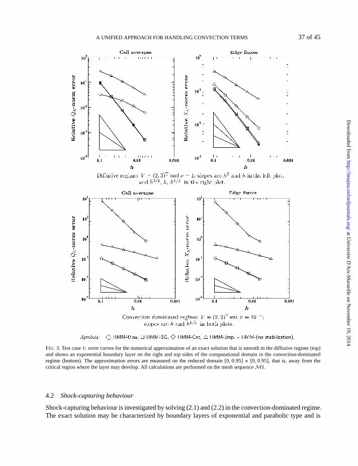
A UNIFIED APPROACH FOR HANDLING CONVECTION TERMS 37 of 45
FIG. 3. Test case 1: error curves for the numerical approximation of an exact solution that is smooth in the diffusive regime (top)and shows an exponential boundary layer on the right and top sides of the computational domain in the convection-dominatedregime (bottom). The approximation errors are measured on the reduced domain [0, 0.95] × [0, 0.95], that is, away from thecritical region where the layer may develop. All calculations are performed on the mesh sequenceM1.
4.2 Shock-capturing behaviour
Shock-capturing behaviour is investigated by solving (2.1) and (2.2) in the convection-dominated regime.The exact solution may be characterized by boundary layers of exponential and parabolic type and is
at Universite D
'Aix-M
arseille on Novem
ber 19, 2014http://im
ajna.oxfordjournals.org/D
ownloaded from

38 of 45 B. DA VEIGA ET AL.
FIG. 4. Shock-capturing test case: the exact solution has an exponential boundary layer on the right and top sides of the computa-tional domain. The calculations are performed on the second mesh of the mesh familyM1 by taking the constant velocity fieldV = (2,3)T andν = 10−4. The numerical solution is displayed at the mesh vertices through linear interpolation. Severe oscil-lations are visible in plot (c) when we use the scheme HMM-(no stabilization), that is, the central mimetic discretization withoutany stabilization (note the different scale along thez-axis). This phenomenon disappears in plot (d) when jump stabilization isturned on using the scheme HMM-Jmp.
approximated on the sequence of meshes ofM1. The numerical solution is plotted at mesh vertices.Vertex values are obtained by interpolating the approximate cell averages provided by the scheme.
4.2.1 Exponential boundary layers.We experimentally investigate how these methods approximatea solution with an exponential boundary layer that forms on those sides of the domain boundary whereV points outward. For this purpose, we solve problem (2.1) and (2.2) with the same data that was usedfor the accuracy benchmark test in the convection-dominated regime, that is, forν = 10−4.
at Universite D
'Aix-M
arseille on Novem
ber 19, 2014http://im
ajna.oxfordjournals.org/D
ownloaded from

A UNIFIED APPROACH FOR HANDLING CONVECTION TERMS 39of 45
In Fig. 4 we compare the numerical solutions produced by the following implementations: HMM-SG, HMM-Upw, HMM-(no stabilization) and HMM-Jmp.
In plots (a) and (b) the nonoscillatory solutions produced by the schemes HMM-SG and HMM-Upw,respectively, are displayed. In contrast, from plot (c) it is evident that, when the calculation is performedusing the HMM-(no stabilization) scheme without any stabilization, the numerical solution suffers fromsevere oscillations. These oscillations disappear when we introduce a stabilizing term in the divergenceequation that is based on the solution’s jump at the mesh edges. However, a great numerical diffusionis introduced by this form of upwinding and the resolution of the boundary layer is poor and generallyworse than that obtained through the other HMM implementations.
4.2.2 Exponential and parabolic boundary layers.OnΩ = ]0, 1[ × ]0, 1[ we numerically solve (2.1)and (2.2) with the Dirichlet boundary conditions
p(x, 0) = (1 − x)3, p(x, 1) = (1 − x)2, p(0, y) = 1, p(1, y) = 0,
andV = (1,0)T in the convection-dominated regime forν = 10−4. The solution has an exponentialboundary layer at the sidex = 1 and two parabolic boundary layers aty = 0 andy = 1. Figure5 showsthe numerical results obtained from calculations using HMM-SG, HMM-Upw, HMM-(no stabilization)and HMM-Jmp. The behaviour is similar to the behaviour documented in Section 4.2.1 for the case of asingle exponential layer.
4.3 Strongly anisotropic heterogeneous and convection-dominated case
In this third example we consider the test case proposed inErnet al.(2009) where the problem (2.1) and(2.2) is solved for a strongly anisotropic and heterogeneous diffusion tensor and a rotating convectionfield. A zeroth-order term proportional top is also present in the model’s equations, and its discretizationis straightforward (see, e.g.,Cangianiet al., 2009). The domainΩ = ]0, 1] × ]0, 1[ is split into foursubdomainsΩ1 = ]0, 2/3[ × ]0, 2/3[, Ω2 = ]0, 2/3[ × ]2/3,1[, Ω2 = ]2/3,1[ × ]2/3,1[ andΩ4 =]2/3,1[ × ]0, 2/3[. The diffusion tensor is diagonal in each subdomain and is characterized by a verysmall value along one principal direction as follows:
Λ =(
10−6 00 1
)in Ω1 andΩ3
and
Λ =(
1 00 10−6
)in Ω2 andΩ4.
Notethat the directions along which diffusion is small are interchanged for adjacent subdomains. Con-vection is given by the clockwise rotating solenoidal fieldV(x, y) = 40(x(2y − 1)(x − 1),−y(2x −1)(y − 1)) and the right-hand side is a gaussian bump positioned at a distance of 0.35 from the domaincentre, given byf (x, y) = 10−2 exp(−(r −0.35)2/0.005)with r 2 = (x−0.5)2+(y−0.5)2. This prob-lem is convection dominated, thus requiring some sort of upwinding in the numerical treatment of theconvection term. Moreover, the exact solution is continuous, but internal layers form near the interfacesthat separate the subdomains due to the small diffusion value in the switching directions. The strongsolution gradients cannot be resolved by the attainable grid sizes and the numerical approximations areexpected to be discontinuous at the internal interfaces.
at Universite D
'Aix-M
arseille on Novem
ber 19, 2014http://im
ajna.oxfordjournals.org/D
ownloaded from

40 of 45 B. DA VEIGA ET AL.
FIG. 5. Shock-capturing test case: the exact solution has an exponential boundary layer on the right side and two parabolic layerson the top and bottom sides of the computational domain. The calculations are performed on the second mesh of the mesh familyM1 by taking the constant velocity fieldV = (1,0)T andν = 10−4. The numerical solution is displayed at the mesh verticesthrough linear interpolation. Severe oscillations are visible in plot (c) when we use the scheme HMM-(no stabilization), that is, thecentral mimetic discretization without any stabilization (note the different scale along thez-axis). This phenomenon disappears inplot (d) when jump stabilization is turned on using the scheme HMM-Jmp.
In the test cases presented in Sections 4.2.1 and 4.2.2 there was no significant difference between thenumerical approximations provided by the cell-based version of the upwind scheme HMM-Upw (see(2.41) and (2.42)), and its edge-based version (see (2.47)–(2.49)). This is no longer the case herein, asillustrated in Fig.6. The calculations, which use the two alternative versions of the HMM-Upw scheme,
at Universite D
'Aix-M
arseille on Novem
ber 19, 2014http://im
ajna.oxfordjournals.org/D
ownloaded from

A UNIFIED APPROACH FOR HANDLING CONVECTION TERMS 41 of 45
FIG. 6. Strongly anisotropic heterogeneous and convection-dominated test case: on a coarse mesh the cell-based upwinding of theconvection provokes spurious oscillations that are completely absent in the edge-based upwinding discretization.
are performed on a grid obtained by a 30× 30 periodic reproduction of the pattern shown in Fig.6(a).Since theexactsolution of this problem is unknown, a reference solution is calculated, for comparison’ssake, on a very fine cartesian grid. The reference solution is displayed in Fig.6(b). The numericalsolution provided by the cell-based upwind scheme is shown in Fig.6(c) and is clearly affected byspurious oscillations. In contrast, this undesirable effect is almost completely absent in the numericalsolution provided by the edge-based upwind scheme, which is shown in Fig.6(d).
It is also worth mentioning the behaviour of these two different implementations of the HMM-Upwscheme as far as minimum and maximum principles are concerned. For this purpose, we recall that
at Universite D
'Aix-M
arseille on Novem
ber 19, 2014http://im
ajna.oxfordjournals.org/D
ownloaded from

42of 45 B. DA VEIGA ET AL.
thenumerical solutions obtained by first-order upwind two-point FV schemes in convection-dominatedproblems are characterized by numerical properties such as positivity, monotonicity, etc. A thoroughinspection of our numerical results reveals that both cell-based and edge-based schemes respect theminimum value, which is zero for the reference solution, and provide 6.6 × 10⁻⁴ and 6.9 × 10⁻⁴,respectively, for the maximum value against a reference value of approximately 6.7×10⁻⁴. Nonetheless,we noted a minimum value of approximately−1.1×10⁻⁵, which corresponds to a numerical undershootof around 1.6%, when we applied the cell-based scheme on a different mesh given by splitting everyother rectangular cell of a 120× 60 regular partition ofΩ into two subtriangles. On this latter mesh,the edge-based upwind scheme was still seen to respect the zero minimum value. We do not showthe other solution plots for these latter calculations because their behaviours are very similar to thoseof the solutions shown in Fig.6. From these qualitative comparisons we deduce that the edge-basedupwind scheme may be more stable and accurate than the cell-based upwind scheme. We also remarkthat the edge-based upwind scheme has the advantage of being fully hybridizable, thus leading to alinear system in the edge unknowns through local variable eliminations such as, for example, in thestatic condensation of mixed finite elements. For these reasons, the edge-based upwind scheme may bepreferable when dealing with stiff problems on coarse meshes.
REMARK 4.2 As a final comment, we observe that, in all of the developed tests, the schemes HMM-(nostabilization) and HMM-Jmp, which satisfy only (AB3-w), do not show particular pathologies for coarsemeshes. Therefore, at least on the basis of the presented tests, theh-small-enough condition appearingin Theorem3.11does not seem to pose a true limitation in practice.
5. Conclusions
We have presented a new family of methods for the numerical approximation to the solution of thesteady convection–diffusion equation. These methods, which are referred to as HMM methods, arebased on a unified formulation for the hybrid FV method, the mixed FV method and the MFD method,and differ mainly in the approximation of the convection term. In particular, we considered centred,upwind, weighted and locally scaled Scharfetter–Gummel-type discretizations for which we provided afull proof of convergence under very general regularity conditions of the solution field and derived anerror estimate when the scalar solution is inH2(Ω).
In the last part of the paper we numerically compared the performance of these schemes on a set oftest cases selected from the literature in both diffusion- and convection-dominated regimes. As expected,the methods, including a centred-type discretization of the convective term, showed a better behaviourin the test cases dominated by diffusion, exhibiting a superconvergence in the approximation of bothscalar and vector variables. On the other hand, such schemes showed a strong loss of convergence ratein the convection-dominated tests, while on those same tests the methods with upwinding or stabiliza-tion exhibited a better behaviour. Finally, we showed a test with strong anisotropy and jumps in thecoefficients. The results seem to suggest that the hybridized formulation gives more stable results forthis kind of problem.
Funding
This work was partially funded by the CentreNational de la Recherche Scientifique(through the GDRMOMAS CNRS/PACEN) and Project VFSitCom (Agence Nationale de la Recherche, ANR-08-BLAN-0275-01).
at Universite D
'Aix-M
arseille on Novem
ber 19, 2014http://im
ajna.oxfordjournals.org/D
ownloaded from

A UNIFIED APPROACH FOR HANDLING CONVECTION TERMS 43of 45
REFERENCES
AAVATSMARK , I., BARKVE, T., BOE, O. & M ANNSETH, T. (1998a) Discretization on unstructured grids forinhomogeneous, anisotropic media. Part I: derivation of the methods.SIAM J. Sci. Comput., 19, 1700–1716.
AAVATSMARK , I., BARKVE, T., BOE, O. & M ANNSETH, T. (1998b) Discretization on unstructured grids forinhomogeneous, anisotropic media. Part II: discussion and numerical results.SIAM J. Sci. Comput., 19, 1717–1736.
ARBOGAST, T., DAWSON, C. N., KEENAN, P. T., WHEELER, M. F. & Y OTOV, I. (1998) Enhanced cell-centeredfinite differences for elliptic equations on general geometry.SIAM J. Sci. Comput., 19, 404–425.
ARNOLD, D. N. & BREZZI, F. (1985) Mixed and nonconforming finite element methods. Implementation, postprocessing and error estimates.RAIRO Model Math. Anal. Numer.,19, 7–32.
ARNOLD, D. N., BREZZI, F., COCKBURN, B. & M ARINI , L. D. (2002) Unified analysis of discontinuousGalerkin methods for elliptic problems.SIAM J. Numer. Anal.,39, 1749–1779.
BARANGER, J., MAITRE, J.-F. & OUDIN, F. (1996) Connection between finite volume and mixed finite elementmethods.RAIRO Model. Math. Anal. Numer.,30, 445–465.
BEIRAO DA VEIGA, L. (2008) A residual based error estimator for the mimetic finite difference method.Numer.Math.,108, 387–406.
BEIRAO DA VEIGA, L. (2010) A mimetic finite difference method for linear elasticity. ESAIMMath. Model.Numer. Anal.,44, 231–250.
BEIRAO DA VEIGA, L., GYRYA, V., L IPNIKOV, K. & M ANZINI , G. (2009a) Mimetic finite difference method forthe Stokes problem on polygonal meshes.J. Comput. Phys.,228, 7215–7232.
BEIRAO DA VEIGA, L., L IPNIKOV, K. & M ANZINI , G. (2010) The mimetic finite difference method for thesteady Stokes problem on polyhedral meshes.SIAM J. Numer. Anal., Available as Technical Report 6PV09/5/0,IMATI-CNR, Pavia, Italy (2009).
BEIRAO DA VEIGA, L., L IPNIKOV, K. & M ANZINI , G. (2009b) Convergence analysis of the high-order mimeticfinite difference method.Numer. Math.,113, 325–356.
BEIRAO DA VEIGA, L. & M ANZINI , G. (2008a) A higher-order formulation of the mimetic finite differencemethod.SIAM J. Sci. Comput., 31, 732–760.
BEIRAO DA VEIGA, L. & M ANZINI , G. (2008b) An a posteriori error estimator for the mimetic finite differenceapproximation of elliptic problems.Int. J. Numer. Methods Eng., 76, 1696–1723.
BERNDT, M., L IPNIKOV, K., MOULTON, J. D. & SHASHKOV, M. (2001) Convergence of mimetic finite differencediscretizations of the diffusion equation.East-West J. Numer. Math., 9, 253–284.
BERTOLAZZI , E. & M ANZINI , G. (2002) Algorithm 817 P2MESH: generic object-oriented interface between 2-Dunstructured meshes and FEM/FVM-based PDE solvers.ACM Trans. Math. Softw.,28, 101–132.
BERTOLAZZI , E. & M ANZINI , G. (2004) A cell-centered second-order accurate finite volume method forconvection–diffusion problems on unstructured meshes.Math. Models Methods Appl. Sci.,8, 1235–1260.
BRENNER, S. & SCOTT, L. (1994)The Mathematical Theory of Finite Element Methods. Berlin: Springer.BREZZI, F., BUFFA, A. & L IPNIKOV, K. (2009) Mimetic finite differences for elliptic problems.Math. Model
Numer. Anal.,43, 277–295.BREZZI, F. & FORTIN, M. (1991)Mixed and Hybrid Finite Element Methods. New York: Springer.BREZZI, F., LIPNIKOV, K. & SHASHKOV, M. (2005a) Convergence of the mimetic finite difference method for
diffusion problems on polyhedral meshes.SIAM J. Numer. Anal., 43, 1872–1896.BREZZI, F., LIPNIKOV, K., SHASHKOV, M. & SIMONCINI , V. (2007) A new discretization methodology for
diffusion problems on generalized polyhedral meshes.Comput. Methods Appl. Mech. Eng., 196, 3682–3692.BREZZI, F., LIPNIKOV, K. & SIMONCINI , V. (2005b) A family of mimetic finite difference methods on polygonal
and polyhedral meshes.Math. Models Methods Appl. Sci.,15, 1533–1551.CANGIANI , A. & M ANZINI , G. (2008) Flux reconstruction and pressure post-processing in mimetic finite differ-
ence methods.Comput. Methods Appl. Mech. Eng., 197, 933–945.
at Universite D
'Aix-M
arseille on Novem
ber 19, 2014http://im
ajna.oxfordjournals.org/D
ownloaded from

44of 45 B. DA VEIGA ET AL.
CANGIANI , A., MANZINI , G. & RUSSO, A. (2009) Convergence analysis of a mimetic finite difference methodfor general second-order elliptic problems.SIAM J. Numer. Anal., 47, 2612–2637.
CHAINAIS -HILLAIRET, C. & DRONIOU, J. (2007) Convergence analysis of a mixed finite volume scheme for anelliptic-parabolic system modeling miscible fluid flows in porous media.SIAM J. Numer. Anal,45, 2228–2258.
CHAINAIS -HILLAIRET, C. & DRONIOU, J. (2009) Finite volume schemes for non-coercive elliptic problems withNeumann boundary conditions.IMA J. Numer. Anal.(to appear) doi: 10.1093/imanum/drp009.
COUDIERE, Y. & M ANZINI , G. (2010) The discrete duality finite volume method for convection–diffusion prob-lems.SIAM J. Numer. Anal.,47, 4163–4192.
DAWSON, C. & A IZINGER, V. (1999) Upwind-mixed methods for transport equations.Comput. Geosci.,3, 93–110.
DOUGLAS JR, J. & ROBERTS, J. E. (1982) Mixed finite element methods for second order elliptic problems.Math.Appl. Comput.,1, 91–103.
DOUGLAS JR, J. & ROBERTS, J. E. (1985) Global estimates for mixed methods for second order elliptic equations.Math. Comput.,44, 39–52.
DRONIOU, J. & EYMARD, R. (2006) A mixed finite volume scheme for anisotropic diffusion problems on anygrid. Numer. Math.,105, 35–71.
DRONIOU, J. & EYMARD, R. (2009) Study of the mixed finite volume method for Stokes and Navier–Stokesequations.Numer. Methods Partial Differ. Equ., 25, 137–171.
DRONIOU, J., EYMARD, R., GALLOUET, T. & H ERBIN, R. (2010) A unified approach to mimetic finite difference,hybrid finite volume and mixed finite volume methods.Math. Models Methods Appl. Sci.,20, 265–295.
ERN, A., STEPHANSEN, A. F. & ZUNINO, P. (2009) A discontinuous Galerkin method with weighted averagesfor advection–diffusion equations with locally small and anisotropic diffusivity.IMA J. Numer. Anal., 29,235–256.
EYMARD, R., GALLOUET, T. & H ERBIN, R. (2000) The finite volume method.Techniques of Scientific Comput-ing, Part III. Handbook for Numerical Analysis(P. Ciarlet & J. L. Lions eds). The Netherlands: North-Holland,pp. 715–1022.
EYMARD, R., GALLOUET, T. & H ERBIN, R. (2009) Discretization of heterogeneous and anisotropic diffusionproblems on general non-conforming meshes, SUSHI: a scheme using stabilisation and hybrid interfaces.IMAJ. Numer. Anal., 30, 1009–1043.
HYMAN , J., MOREL, J., SHASHKOV, M. & STEINBERG, S. (2002) Mimetic finite difference methods for diffusionequations.Comput. Geosci., 6, 333–352.
JAFFRE, J. (1984) Decentrage et elements finis mixtes pour les equations de diffusion–convection.Calcolo, 21,171–197.
JAFFRE, J. & ROBERTS, J. E. (1985) Upstream weighting and mixed finite elements in the simulation of miscibledisplacements.RAIRO Model. Math. Anal. Numer.,19, 443–460.
KUZNETSOV, Y., L IPNIKOV, K. & SHASHKOV, M. (2005) The mimetic finite difference method on polygonalmeshes for diffusion-type problems.Comput. Geosci., 8, 301–324.
LIPNIKOV, K., SHASHKOV, M. & Y OTOV, I. (2009) Local flux mimetic finite difference methods.Numer. Math.,112, 115–152.
MANZINI , G. & RUSSO, A. (2008) A finite volume method for advection–diffusion problems in convection-dominated regimes.Comput. Methods Appl. Mech. Eng., 197, 1242–1261.
RAPIN, G. & L UBE, G. (2004) A stabilized scheme for the Lagrange multiplier method for advection–diffusionequations.Math. Models Methods Appl. Sci.,14, 1035–1060.
RIVIERE, B. (2008)Discontinuous Galerkin Methods for Solving Elliptic and Parabolic Equations: Theory andImplementation. Philadelphia, PA: SIAM.
RUSSELL, T. F. & WHEELER, M. F. (1983) Finite element and finite difference methods for continuous flowsin porous media.The Mathematics of Reservoir Simulation(R. E. Ewing ed.). Philadelphia, PA: SIAM,pp. 35–106.
at Universite D
'Aix-M
arseille on Novem
ber 19, 2014http://im
ajna.oxfordjournals.org/D
ownloaded from

A UNIFIED APPROACH FOR HANDLING CONVECTION TERMS 45of 45
SCHARFETTER, D. L. & GUMMEL , H. K. (1969) Large signal analysis of a silicon read diode.IEEE Trans.Electron Devices, 16, 64–77.
VOHRALIK , M. (2006) Equivalence between lowest-order mixed finite element and multi-point finite volume meth-ods on simplicial meshes.Math. Model. Numer. Anal.,40, 367–391.
WHEELER, M. F. & Y OTOV, I. (2006) A multipoint flux mixed finite element method.SIAM J. Numer. Anal., 44,2082–2106.
YOUNES, A., ACKERER, P. & CHAVENT, G. (2004) From mixed finite elements to finite volumes for ellipticPDEs in two and three dimensions.Int. J. Numer. Methods Eng., 59, 365–388.
at Universite D
'Aix-M
arseille on Novem
ber 19, 2014http://im
ajna.oxfordjournals.org/D
ownloaded from