a user manual for jmarkov package

A User Manual for jMarkov Package

Trabajo de Tesispresentado al

Departamento de Ingeniería Industrial

por

Marco Sergio Cote Vicini

Asesor: Raha Akhavan-TabatabaeGerman Riaño

Para optar al título deIngeniero Industrial

Ingeniería IndustrialUniversidad de Los Andes

Junio 2011

To my father and my mother for their constant support, to my sister

for her unconditional love.

ii

Acknowledge

I want to acknowledge the work done by German Riaño, Juan Fernando Perez,

Andres Sarmiento and Julio Goez who are the developers of the jMarkov software

and were always there to support me and answerer my in�nite questions.

Also I want to acknowledge all the support and guidance given by German, Raha

and Andres through this last year. Without their help and advice this document

have never been done.

iii

Table of Contents

Dedicatoria ii

Acknowledge iii

List of Figures vi

Abstract vii

I Introduction 1

II Background 4

2.1 Literature Review . . . . . . . . . . . . . . . . . . . . . . . . . . . . 4

2.2 Markov Chains . . . . . . . . . . . . . . . . . . . . . . . . . . . . . . 6

2.3 Quasi Birth and Death Process (QBD) . . . . . . . . . . . . . . . . 7

2.4 Phase Type Distributions (PH Distributions) . . . . . . . . . . . . . 9

2.4.1 Fitting Algorithms . . . . . . . . . . . . . . . . . . . . . . . . 12

2.5 Markov Decision Process (MDP) . . . . . . . . . . . . . . . . . . . . 12

2.5.1 Finite Horizon Problems . . . . . . . . . . . . . . . . . . . . 13

2.5.2 In�nite Horizon Problems . . . . . . . . . . . . . . . . . . . . 14

2.5.3 Continuous Time Markov Decision Processes . . . . . . . . . 15

2.5.4 Event Modeling . . . . . . . . . . . . . . . . . . . . . . . . . 15

III Work Process 18

IV User Manual 22

4.1 Programming Knowledge . . . . . . . . . . . . . . . . . . . . . . . . 22

4.2 Structure Description . . . . . . . . . . . . . . . . . . . . . . . . . . 23

4.2.1 jMarkov.basic . . . . . . . . . . . . . . . . . . . . . . . . . . 23

iv

4.2.2 jMarkov and jQBD . . . . . . . . . . . . . . . . . . . . . . . 25

4.2.3 jPhase . . . . . . . . . . . . . . . . . . . . . . . . . . . . . . 28

4.2.4 jMDP . . . . . . . . . . . . . . . . . . . . . . . . . . . . . . . 32

4.3 Modeling Process . . . . . . . . . . . . . . . . . . . . . . . . . . . . 34

4.3.1 jMarkov.basic . . . . . . . . . . . . . . . . . . . . . . . . . . 34

4.3.2 jMarkov . . . . . . . . . . . . . . . . . . . . . . . . . . . . . 40

4.3.3 jQBD . . . . . . . . . . . . . . . . . . . . . . . . . . . . . . . 46

4.3.4 jPhase . . . . . . . . . . . . . . . . . . . . . . . . . . . . . . 50

4.3.5 jMDP . . . . . . . . . . . . . . . . . . . . . . . . . . . . . . . 57

V Applications in Real Life Problems 64

VI Conclusions 66

v

List of Figures

1 Taxonomy for MDP problems . . . . . . . . . . . . . . . . . . . . . . 12

2 User's Manual Architecture . . . . . . . . . . . . . . . . . . . . . . . 20

3 The main classes of the basic package . . . . . . . . . . . . . . . . . . 24

4 The main classes of the jMarkov modeling package . . . . . . . . . . 25

5 BuildRS algorithm . . . . . . . . . . . . . . . . . . . . . . . . . . . . 26

6 The User Interface of jMarkov and jQBD . . . . . . . . . . . . . . . . 27

7 The Toolbar . . . . . . . . . . . . . . . . . . . . . . . . . . . . . . . . 27

8 The Interface Views . . . . . . . . . . . . . . . . . . . . . . . . . . . . 28

9 The jPhase Main Classes . . . . . . . . . . . . . . . . . . . . . . . . . 29

10 The jPhase Interface . . . . . . . . . . . . . . . . . . . . . . . . . . . 31

11 Createing a New PH Distribution . . . . . . . . . . . . . . . . . . . . 32

12 Choosing a Fitting Process . . . . . . . . . . . . . . . . . . . . . . . . 32

13 The jMDP Main Classes . . . . . . . . . . . . . . . . . . . . . . . . . 33

vi

Abstract

This document presents the user manual of the jMarkov software, an object-

oriented modeling software designed for the analysis of stochastic systems in steady

state. It allows the user to create Markov models of arbitrary size with its component

jMarkov. It also provides the tools to model quasi-birth-death process. processes

with its jQBD component.

Further development of the software has created two new modules. jPhase allows

representation of phase-type distributions that are useful when representing real-life

systems, and jMDP is a module for modeling and solving Markov decision processes

and dynamic programming problems.

vii

Chapter I

Introduction

When analyzing real-life stochastic systems, using analytical models is often eas-

ier, cheaper and more e�ective than studying the physical system or a simulation

model of it. The stochastic modeling is a powerful tool that helps the analysis and

optimization of stochastic systems.

However, the use of stochastic modeling is not widespread in today's industries

and among practitioners. This lack of acceptance has two main causes. The �rst is

the curse of dimensionality, which is de�ned by the number of states required to de-

scribe a system. This number grows exponentially as the size of the system increases.

The second is the lack of user-friendly and e�cient software packages that allow the

modeling of the problem without involving the user with the implementation of the

solution algorithms necessary to solve it.

The curse of dimensionality is a constant problem that has been addressed by

di�erent approaches over time, but it is outside the scope of this document. The

focus of this it is the latter issue, the lack of user-friendly and e�cient software

packages. We propose a generic solver that enables the user to focus on modeling

without becoming involved in the complexity required by the solution methods.

1

jMarkov is an object-oriented framework for stochastic modeling with four com-

ponents: jMarkov, which models Markov chains; jQBD, which models quasi-birth-

death processes; jPhase, which models phase-types distributions; and jMDP, which

models Markov decision processes (MDPs). The main contribution of this frame-

work is the separation of modeling steps from the solution algorithms. The user can

concentrate on modeling the problems and choose from a set of solvers at his or her

convenience. The structure of the software package allows third-party developers to

plug in their own solvers.

The modeling software does not use external plain �les, like ".txt" or ".dat" �les,

written with speci�c commands; rather, it is based on object-oriented programming

(OOP) [1], which enables the encapsulation of entities in classes and exposes its

functionality independently of its internal implementation. This has many bene�ts,

including, �rst, the analogy between the mathematical elements and their compu-

tational representation; second, the exploration algorithm, which �nds all the states

in the chain, avoiding possible mistakes the user can make by manual de�nition in

very large systems; and, third, that the software is based in Java, so the user need

not deal with technical processes like memory allocations.

Although jMarkov was developed a few years ago, stochastic modeling is not

widespread. Most people still prefer other system-analyzing tools like simulations.

jMarkov has not �xed the initial problem of creating an user-friendly software for

motivating the use of stochastic modeling. The main reason for this is the lack of

a simple and easy reading manual. The existing documentation has an academic

and computer-science approach, confusing to people new to stochastic modeling and

lacking extensive programming knowledge. Its examples require signi�cant software

understanding, making jMarkov look like a complex tool, when it is actually quite

2

easy to work with. The existing user manual is presented in this document.

The present document is organized as follows. Section 2 provides a brief mathe-

matical background needed to understand the other sections, as well as descriptions

of the notations used. Readers who feel comfortable with the topic can skip this

section without any break in continuity. Section 3 describes the work done to create

the new manual. Section 4 is the user manual. It explains the main computational

elements that the user needs to know to build a model and describes the handling of

di�erent problems with an example. Section 5 presents references to real industry

problems that have been and are being solved using the software. Section 6 presents

general conclusions.

3

Chapter II

Background

In this section we give a short explanation of the main mathematical topics the

reader has to be familiar with to facilitate understanding of the software. We do

not intend to explain the topics, just to present a quick review. We also provide

references for readers who want to read more about these topics. And we present

the literature review done for look onder software packages similar to jMarkov.

It is important to mention that to ful�ll the main purpose of the document-to

create an e�ective user manual for jMarkov-this chapter has been taken from the

thesis done by jMarkov developers. We want to acknowledge credit for the following

pages to German Riaño [30], Juan Fernando Perez [47], Andres Sarmiento [48] and

Julio Goez [45].

2.1 Literature Review

Several packages for solving stochastic processes, such as MAMSolver [2], MGMTool

[3], SMAQ [4], Qnap2 [5], and XMarca [6], can be found but them have a focus on the

solution algorithm rather than ours, which has a modeling purpose. They are tools

that implement analytical algorithms to solve queuing problems. Additionally, there

can be found the SIMULA language [7], which is the �rst modeling tool based on

4

OOP. Others, such as MARCA [8], SMART [9], PROBMELA [10] and Generalized

Markovian Analysis of Timed Transitions Systems [11], allow building and analyzing

Markov chains, but they are not based on OOP, so the modeling becomes harder

for beginners to the subject.

The program most similar to jMarkov is probably SHARPE [24], which mod-

els di�erent types of systems including combinatorial ones, such as fault trees and

queuing networks, and state-space ones, such as Markov and semi-Markov reward

models, as well as stochastic Petri nets. It also computes steady-state, transient and

interval measures. The main di�erence between these software packages and ours is

that jMarkov has a component for Markov decision processes (MDPs) that allows

not only analysis, but also optimization, of the systems under study.

From another perspective, some stochastic linear programming languages have

been developed, such as Xpress-SP [12], extensions for AMPL [13] and SAMPL/SPInE

[14]. These are not fully comparable to the framework presented in this document,

because they have some speci�c limitations and are not very open to reach to any

type of stochastic modeling.

The literature review speci�c on MDP modeling software includes a program

able to solve them, winQSB [15], into which the user needs to input the transition

matrices for each action. Other works include MDPLab [16], an educational tool

developed by Lamond to test di�erent algorithms, a toolbox for Matlab to handle

MDPs [17] and a variety of software made in academia, such as Pascal Poupart

from University of Waterloo [18], Trey Smith's with his software called ZMDP [19],

Anthony R. Cassandra from Brown University [20], Matthijs Spaan from Universiteit

van Amsterdam with his software called perseus [21], Tarek Taha with a set of tools

for solving POMDP (partially observable MDP) [22] and an open source project

5

called Caylus [23]. However, all of these software packages are primarily focused

on the solutions algorithm, and all of them use plain �les as inputs for building

the Markov chain. Our proposed software package centers the e�ort on facilitating

the modeling aspect of the problem providing a pre-coded solution algorithms while

also leaving open the possibility of coding new solvers, such as the ones mentioned

above.

2.2 Markov Chains

Suppose we observe some characteristic of a system. Let X(t) be the value of the

system characteristic at time t, this value is not known with certainty before time

t so it can be viewed as a random variable. This characteristic that describes the

system in a speci�c time is called state. A state changes its value, when an event

occurs. The probability of passing from one state to another is called the transition

probability. A stochastic process is simply a description of the relation between the

random variables [25].

A Discrete Time Markov Chain (DTMC) is a special type of stochastic process

that meets the Markovian property. The property de�nes a process where the condi-

tional distribution of any future stateX(t+1), given the past statesX(0), ..., X(t−1)

and the present state X(t) , is independent of the past states and depends only on

the present state [25].

From now on we limit our description to Continuous Time Markov Chain (CTMC),

although jMarkov can also handle Discrete Time Markov Chains (DTMC) as well.

Let {X(t), t ≥ 0} be a CTMC, with �nite State Space S and generator matrix

Q, with components

qij = limt↓0

P {X(t) = j|X(0) = i} i, j ∈ S.

6

It is well known that this generator matrix, along with the initial conditions, com-

pletely determines the transient and stationary behavior of the Markov Chain [26].

The diagonal components qii are non-positive and represent the exponential hold-

ing rate for state i, whereas the o� diagonal elements qij represent the transition

rate from state i to state j.

The transient behavior of the system is described by the matrix P(t) with com-

ponents

pij(t) = P {X(t+ s) = j|X(s) = i} i, j ∈ S.

This matrix can be computed as

P(t) = eQt t > 0.

For an irreducible chain, the stationary distribution π = [π1, π2, . . . , ] is determined

as the solution to the following system of equations

πQ = 0

π1 = 1,

where 1 is a column vector of ones.

2.3 Quasi Birth and Death Process (QBD)

Consider a Markov process {X(t) : t ≥ 0} with a two dimensional state space

S = {(n, i) : n ≥ 0, 1 ≤ i ≤ m}. The �rst coordinate n is called the level of the

process and the second coordinate i is called the phase. We assume that the number

of phases m is �nite. In applications, the level usually represents the number of

items in the system, whereas the phase might represent di�erent stages of a service

process.

7

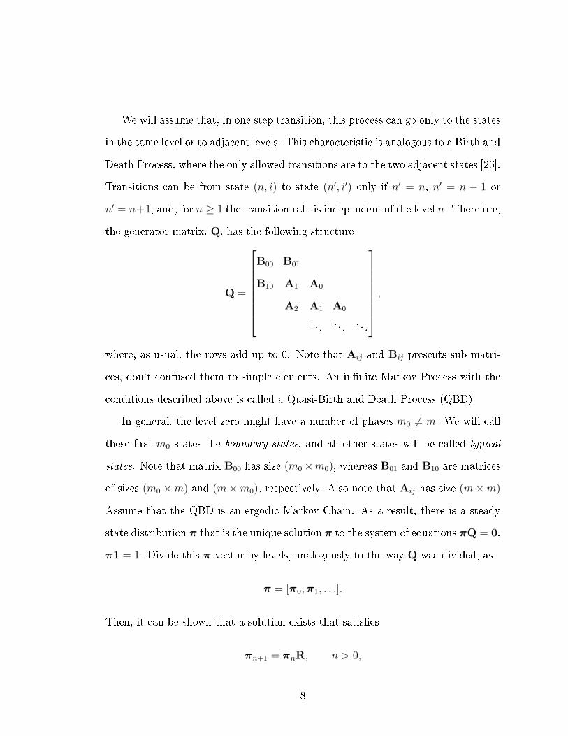
We will assume that, in one step transition, this process can go only to the states

in the same level or to adjacent levels. This characteristic is analogous to a Birth and

Death Process, where the only allowed transitions are to the two adjacent states [26].

Transitions can be from state (n, i) to state (n′, i′) only if n′ = n, n′ = n − 1 or

n′ = n+1, and, for n ≥ 1 the transition rate is independent of the level n. Therefore,

the generator matrix, Q, has the following structure

Q =

B00 B01

B10 A1 A0

A2 A1 A0

. . . . . . . . .

,

where, as usual, the rows add up to 0. Note that Aij and Bij presents sub matri-

ces, don't confused them to simple elements. An in�nite Markov Process with the

conditions described above is called a Quasi-Birth and Death Process (QBD).

In general, the level zero might have a number of phases m0 6= m. We will call

these �rst m0 states the boundary states, and all other states will be called typical

states. Note that matrix B00 has size (m0×m0), whereas B01 and B10 are matrices

of sizes (m0 ×m) and (m×m0), respectively. Also note that Aij has size (m×m)

Assume that the QBD is an ergodic Markov Chain. As a result, there is a steady

state distribution π that is the unique solution π to the system of equations πQ = 0,

π1 = 1. Divide this π vector by levels, analogously to the way Q was divided, as

π = [π0,π1, . . .].

Then, it can be shown that a solution exists that satis�es

πn+1 = πnR, n > 0,

8

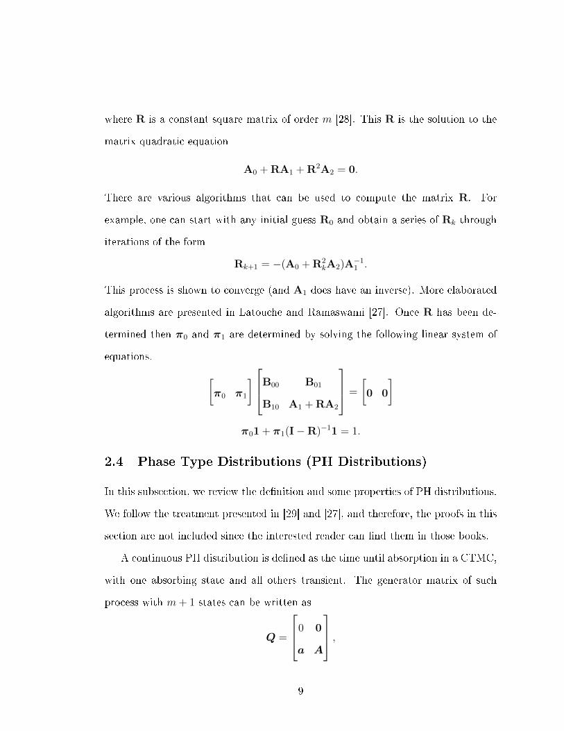
where R is a constant square matrix of order m [28]. This R is the solution to the

matrix quadratic equation

A0 +RA1 +R2A2 = 0.

There are various algorithms that can be used to compute the matrix R. For

example, one can start with any initial guess R0 and obtain a series of Rk through

iterations of the form

Rk+1 = −(A0 +R2kA2)A

−11 .

This process is shown to converge (and A1 does have an inverse). More elaborated

algorithms are presented in Latouche and Ramaswami [27]. Once R has been de-

termined then π0 and π1 are determined by solving the following linear system of

equations. [π0 π1

]B00 B01

B10 A1 +RA2

=

[0 0

]

π01+ π1(I−R)−11 = 1.

2.4 Phase Type Distributions (PH Distributions)

In this subsection, we review the de�nition and some properties of PH distributions.

We follow the treatment presented in [29] and [27], and therefore, the proofs in this

section are not included since the interested reader can �nd them in those books.

A continuous PH distribution is de�ned as the time until absorption in a CTMC,

with one absorbing state and all others transient. The generator matrix of such

process with m+ 1 states can be written as

Q =

0 0

a A

,

9

where A is a square matrix of size m, a is a column vector of size m and 0 is a row

vector of zeros. Here, the the �rst entry in the state space represents the absorbing

state. As the sum of the elements on each row must be equal to zero, a is determined

by

a = −A1,

where 1 is a column vector of ones. In order to completely determine the process,

the initial probability distribution is de�ned, and can be partitioned, in an similar

way to the generator matrix, as [α0 α

],

where α0 is the probability that the process starts in the absorbing state 0. Since

the sum of all the components in the initials conditions vector must be equal to 1,

α0 is determined by

α0 = 1−α1.

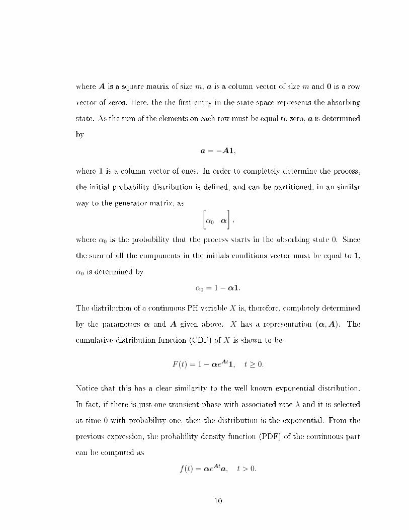
The distribution of a continuous PH variable X is, therefore, completely determined

by the parameters α and A given above. X has a representation (α,A). The

cumulative distribution function (CDF) of X is shown to be

F (t) = 1−αeAt1, t ≥ 0.

Notice that this has a clear similarity to the well-known exponential distribution.

In fact, if there is just one transient phase with associated rate λ and it is selected

at time 0 with probability one, then the distribution is the exponential. From the

previous expression, the probability density function (PDF) of the continuous part

can be computed as

f(t) = αeAta, t > 0.

10

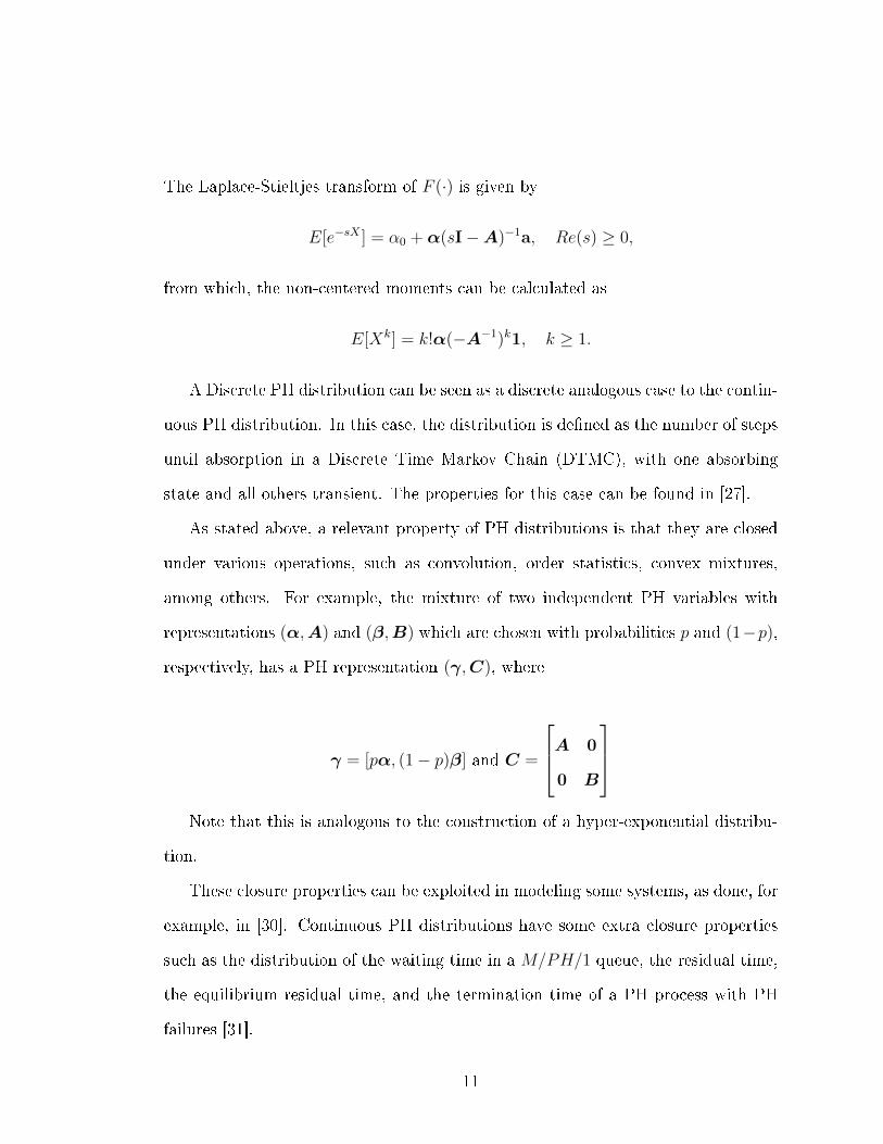
The Laplace-Stieltjes transform of F (·) is given by

E[e−sX ] = α0 +α(sI−A)−1a, Re(s) ≥ 0,

from which, the non-centered moments can be calculated as

E[Xk] = k!α(−A−1)k1, k ≥ 1.

A Discrete PH distribution can be seen as a discrete analogous case to the contin-

uous PH distribution. In this case, the distribution is de�ned as the number of steps

until absorption in a Discrete Time Markov Chain (DTMC), with one absorbing

state and all others transient. The properties for this case can be found in [27].

As stated above, a relevant property of PH distributions is that they are closed

under various operations, such as convolution, order statistics, convex mixtures,

among others. For example, the mixture of two independent PH variables with

representations (α,A) and (β,B) which are chosen with probabilities p and (1−p),

respectively, has a PH representation (γ,C), where

γ = [pα, (1− p)β] and C =

A 0

0 B

Note that this is analogous to the construction of a hyper-exponential distribu-

tion.

These closure properties can be exploited in modeling some systems, as done, for

example, in [30]. Continuous PH distributions have some extra closure properties

such as the distribution of the waiting time in a M/PH/1 queue, the residual time,

the equilibrium residual time, and the termination time of a PH process with PH

failures [31].

11

2.4.1 Fitting Algorithms

In the last twenty years, the problem of �tting the parameters of a PH distribution

has received great attention from the applied probability community. There are

di�erent approaches that, as noted in [32], can be classi�ed in two major groups:

maximum likelihood methods and moment matching techniques. Nevertheless, al-

most all the algorithms designed for this task have an important characteristic in

common: they reduce the set of distributions to be �tted from the whole PH set to

a special subset.

The maximum likelihood algorithms we review were by Asmussen et. al. [33],

Khayari et. al. [34], and Thümmler et. al. [35], as well as the moment matching

algorithms by Telek and Heindl [36], Osogami and Harchol [37], and Bobbio et.

al. [38].

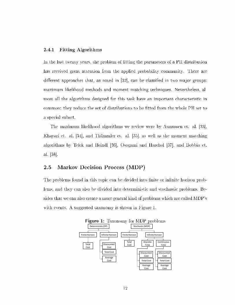
2.5 Markov Decision Process (MDP)

The problems found in this topic can be divided into �nite or in�nite horizon prob-

lems, and they can also be divided into deterministic and stochastic problems. Be-

sides that we can also create a more general kind of problems which are called MDP's

with events. A suggested taxonomy is shown in Figure 1.

Figure 1: Taxonomy for MDP problemsDeterministic (DP) Stochastic (MDP)

Infinite HorizonFinite Horizon Infinite HorizonFinite Horizon

TotalCost

TotalCost

DiscreteTime

Continuous Time

Average Cost

Total Cost

DiscountedCost

Average Cost

Total Cost

DiscountedCost

Average Cost

Total Cost

DiscountedCost

12

2.5.1 Finite Horizon Problems

We will show how a �nite horizon Markov decision process is built (for a com-

plete reference see Puterman [39] and Bertsekas [40]). Consider a discrete state

space, discrete time epochs or stages and a bivariate random process {(Xt, At), t =

0, 1, . . . , T − 1}. Each of the variable Xt ∈ St represents the state of the system at

stage t, and each At ∈ At is the action taken at that stage. The quantity T <∞ is

called the horizon of the problem.

The sets St and At represent the feasible states and actions at stage t, and

we assume that both are �nite. Let Ht be the history of the process up to time

t, i.e. Ht = (X0, A0, X1, A1, . . . , Xt−1, At−1, Xt). The dynamics of the system are

governed by a state in which an action is taken, leading the system to another

state according to a probability distribution. In general, the resulting state after

a transition from one state to another when the process is moved up to the next

stage depends on the history and the action taken in the previous stage. The

system satis�es the Markov property which implies P{Xt+1 = j|Ht = h,At = a} =

P{Xt+1 = j|Xt = i, At = a} = pijt(a). A decision rule is a function πt that, given a

history realization, assigns a probability distribution over the set A. A sequence of

decision rules π = (π0, π1, . . . , πT ) is called a policy . A policy π is called Markovian

if given Xt all previous history becomes irrelevant, that is

Pπ{At = a|Ht = h} = Pπ{At = a|Xt = i},

where Pπ denotes the transition probability distribution following policy π. A

Markovian policy π is called deterministic if there is a function ft(i) ∈ A such

13

that

Pπ{At = a|Xt = i} =

1 if a = f(i)

0 otherwise.

For each action a taken at state i and stage t, a �nite cost ct(i, a) is incurred.

Consequently it is possible to de�ne a total expected cost vπt (i) incurred from time

t to the �nal stage T following policy π; this is called the value function

vπt (i) = Eπ

[T∑s=t

cs(Xs, As)∣∣∣Xt = i

], i ∈ S0 (1)

where Eπ is the expectation operator following the probability distribution associ-

ated with policy π.

2.5.2 In�nite Horizon Problems

Consider a discrete space discrete time bivariate random process{(Xt, At), t ∈ N

}.

In particular we will assume that the the system is time homogeneous, this means

that at every stage the state space and action space remain constant and the tran-

sition probabilities are independent of the stage. i.e. pijt(a) = pij(a) = P{Xt+1 =

j|Xt = i, At = a} for all stages. Consequently, a policy π = (π0, π0, . . .) must also

be time homogeneous. Costs are also time homogeneous and ct(i, a) = c(i, a) stands

for the cost incurred when action a is taken in state i at any stage. Besides the total

cost objective function presented in the �nite horizon problem, it is customary to

de�ne two other objective functions namely, discounted cost and average cost. The

respective value functions under a policy π are

vπα(i) = Eπ

[∞∑t=0

αtc(Xt, At)∣∣∣X0 = i

], i ∈ S,

for the discounted cost where 0 < α < 1,

vπ(i) = Eπ

[∞∑t=0

c(Xt, At)∣∣∣X0 = i

], i ∈ S,

14

for the total cost, and

vπ(i) = limT→∞

1

TEπ

[T∑t=0

c(Xt, At)∣∣∣X0 = i

], i ∈ S,

for the average cost.

2.5.3 Continuous Time Markov Decision Processes

Consider an in�nite horizon problem with time-homogeneity, where the set{(X(t), A(t)

), t ≥

0}is the bivariate process that describes the state of the system and the action taken

at time t, on a continuous time space. The continuous time in�nite horizon problem

is denoted by CTMDP. Time-homogeneous transitions between states are described

by a transition rate λij(a) = limh→0 P{X(t + h) = j|X(t) = i, A(t) = a}. The

Markovian property implies that the time between transitions from one state to an-

other has an exponential distribution with parameter λi(a) equal to the sum of the

exit rates from the former state. This implies that a transition occurs only when

the state of the system X(t) changes and no self transitions are allowed. We de�ne

rate λ such that λ ≥ λ(i, a) for all states and actions. Costs can be lump costs

c̃(i, a) incurred in the instant when an action is taken and can also be continuously

incurred at rate γ(i, a) while remaining at state i.

2.5.4 Event Modeling

In this subsection we introduce the MDP's with events (for complete reference see

the work of Becker [41], Mahadevan [42], and Feinberg [43]) in order to show that the

process with events is equivalent to another process without events such as the ones

described earlier in this section. The mathematical model presented is an extension

of the mathematical models explained before in the sense that the same problems

can be represented in both. The diference lies that in the problems with event we

15

need to condition each transition to the event triggering it. The advantage of such a

presentation is that conditioning reduces the reachable set for each state and permits

an easier characterization of the system dynamics.

For the mathematical model with events, consider the discrete time random

process{(Xt, At, Et), t = 0, 1, . . . , T − 1

}, where Xt represents the state of the

system, At represents the action taken, and Et is the event that occurs at stage t (as

a consequence of the current state and the action taken) that triggers the transition

to Xt+1.We call the set of events that can occur at stage t, Et(i, a). The history of the

process up to stage t, is de�ned as Ht = (X0, A0, E0 . . . , Xt−1, At−1, Et−1, Xt). The

Markovian behavior of the system implies that P{Xt+1 = j|Ht = h,At = a,Et =

e} = P{Xt+1 = j|Xt = i, At = a,Et = e}. Consequently the dynamics can be

described by transition probabilities de�ned as pijt(a, e) = P{Xt+1 = j|Xt = i, At =

a,Et = e} that describe the conditional probability of reaching state j in the set of

reachable states St(i, a, e), given that the current state is i, action a is chosen and

given that event e occurs. The actions also present a Markovian property in the

sense that P{At = a|Ht = h} = P{At = a|Xt = i}. Finally, we assume that the

occurrence of events follows the Markov property. i.e.

P{Et = e|Ht = h,At = a} = P{Et = e|Xt = i, At = a},

e ∈ Et(i, a).

Let ct(i, a, e) be the cost incurred by taking action a at stage t from state i and

pt(e|i, a) = P{Et = e|Xt = i, At = a} be the conditional probability of occurrence

of event e at stage t.

16

In the �nite horizon problem, the value function is de�ned as

vπt (i) = Eπ

[T∑s=t

cs(Xs, As, Es)∣∣∣Xt = i

],

i ∈ S0, t = 0, 1, . . . , T − 1.

17

Chapter III

Work Process

As stated before, the jMarkov project lacks a user manual by which any person can

learn how to model with the program. When the software was coded, each of the

designers wrote a document for each component that tried to explain that modeling

process. But as user manuals, the documents have some problems.

They mostly focus on the package structure that is the software architecture.

In them, the user can �nd detailed explanations of all the classes' codes, as well

as the relationships between them. Although this is important for a designer, it

is unnecessary information for the user, who does not need to know the internal

processes of the software.

The documents also explain the modeling and solving algorithms used by the

software. We believe this is an excessively academic approach. It is very important

to understand which algorithms we are using in the software, but new users and

beginners to the subject will �nd this unnecessary information.

Finally, the examples provided in the documents are composed of just the coding.

They need to be explained so users can fully understand what they have to do to

work with jMarkov. The examples must be written for beginners, not knowledgeable

users.

18

The purpose of the software is to help stochastic modeling become widespread

and 'widespread' does not mean within computer science or academic communities,

but instead in industry. We need to make the manuals as simple as they can be, so

that people with a minimum knowledge of programming and the basic concepts in

stochastic modeling can use them to analyze small systems. We hope that this way,

in time, more and more people will become interested in the software and will use

it for more complex problems.

Thus we decided to create a user manual that will help users understand jMarkov

and realize how easy it is to work with. This manual gives the steps for modeling

with the software. It does not explain the internal working; it only provides the

information a user really needs to solve a problem. This explanation will consist of

a description of the classes the user will work with, as well as one example explaining

the steps for working with the tool. Through the document we will provide references

to other documents written for users who want to learn about jMarkov's internal

functions. We used the following process to write the manual:

1. Read the existing documents to see what had already been done toward the

goal writing a user manual. From those documents we adapted some informa-

tion as mathematical background.

2. Read the code and the existing examples to understand the internal working

of the software and to determine which parts were important to explain and

which were not.

3. Held meetings with the designers of the software to answer questions about

it. During those meetings we con�rmed the need for a user manual, since the

only way to completely understand the software was by talking to its authors.

19

4. Solved small problems in each component to determine the best way to explain

the process with jMarkov.

5. Translated the modeling steps into simple less technical words so that anyone

would to understand them.

As a result, we realized that to understand how jMarkov works, people would

need to have some essential programming knowledge, knowledge of basic concepts

of structure and ability to learn the modeling process by following a series of steps.

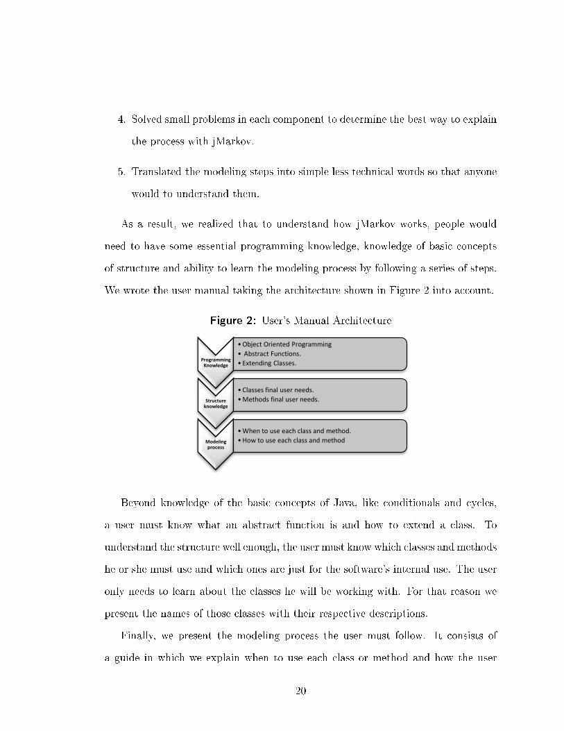
We wrote the user manual taking the architecture shown in Figure 2 into account.

Figure 2: User's Manual Architecture

Programming Knowledge

•Object Oriented Programming

• Abstract Functions.

• Extending Classes.

Structure knowledge

•Classes final user needs.

•Methods final user needs.

Modeling process

•When to use each class and method.

•How to use each class and method

Beyond knowledge of the basic concepts of Java, like conditionals and cycles,

a user must know what an abstract function is and how to extend a class. To

understand the structure well enough, the user must know which classes and methods

he or she must use and which ones are just for the software's internal use. The user

only needs to learn about the classes he will be working with. For that reason we

present the names of those classes with their respective descriptions.

Finally, we present the modeling process the user must follow. It consists of

a guide in which we explain when to use each class or method and how the user

20

should use them. This is followed by an example to better illustrate the point for

the reader.

21

Chapter IV

User Manual

4.1 Programming Knowledge

Java is a high-level programming language created by Sun Microsystems [1]. It

implements an object-oriented approach, the main idea of which can be explained

as "divide and conquer." It assumes that every software program can be divided

into elements or objects, which can be coded separately and then connected to the

others to create a program. This approach is very useful when working with massive

problems.

The object-oriented programming is based on four key principles: abstraction,

encapsulation, inheritance and polymorphism. An excellent explanation of OOP

and the Java programming language can be found in [1].

The abstraction capability is the one that we take the most advantage of for pro-

gramming jMarkov. It consists of the creation of abstract functions and extending

abstract classes.

An abstract function is one in which only the input parameter must be de�ned,

and the output type is returned without coding the function implementation. The

modeler can use an abstract function to program the di�erent algorithms, which

22

work the same without taking into account the di�erent implementations the ab-

stract elements can have.

Extending abstract classes consists of creating general classes that will later help

code particular ones. In a general class we code the algorithms and the abstract

functions. Later, when the user wants to model something, he just needs to extend

an abstract class. By doing so, he must code the abstract functions in the extending

class, so the model can compile and run. Thanks to this, the user does not need

to worry about the coding the extended class; he only needs to be concerned with

coding the few abstract functions.

4.2 Structure Description

In this section we discuss the classes that are part of the modeling process and that

have a direct relationship to the user. The focus of this document is to give new

users the key elements necessary to model with jMarkov and to give an idea of the

software's capabilities. If the reader wants details about the solving packages or the

architecture of the coding in the software, please refer to the reference provided in

each subsection. The following subsections describe each of the important packages,

limiting the explanation to the de�nition of the classes the user needs in order to

create a model.

4.2.1 jMarkov.basic

This package is a collection of classes designed to represent the most basic elements

that interact in any kind of Markov chain or MDP. Figure 3 shows the name of the

main classes in the packages that the user should extend to model a problem.

The state class represents a state in a Markov Chain or MDP. The user of the

class should establish the coding convention and code the compareTo method. In the

23

Figure 3: The main classes of the basic package

jmarkov.basic

ActionEventState

PropertiesEventPropertiesState PropertiesAction

compareTo method the user should give a formula of how the computer must organize

the states. In other words, when comparing two states, the system must determine

which is larger. This is done to create an organized data structure to facilitate

internal searching. The coding convention means that the user should code the data

structure, where the states are going to be saved, while coding the construction

method on the extended class. That data structure, along with the compareTo, must

be established. A complete element order is needed since, for e�ciency, jMarkov

works with ordered sets.

The package also provides a class, called PropertiesState, with a default order

process to do general-problem modeling. It has all the methods implemented in

the state class and it orders the states by an array of integer-valued properties, so

the user does not have to be concerned with the structure or the comparison. In

conclusion, if the state can be represented with a vector of integers describing its

properties, then it might be easier to implement PropertiesState class rather than

state class.

The same situation works with the Event class versus PropertiesEvent class and

Action class versus PropertiesAction class. The class Event allows the user to de�ne

the implementation of the events that can alter the states of the Markov chain. The

class Action represents a single action in MDP.

24

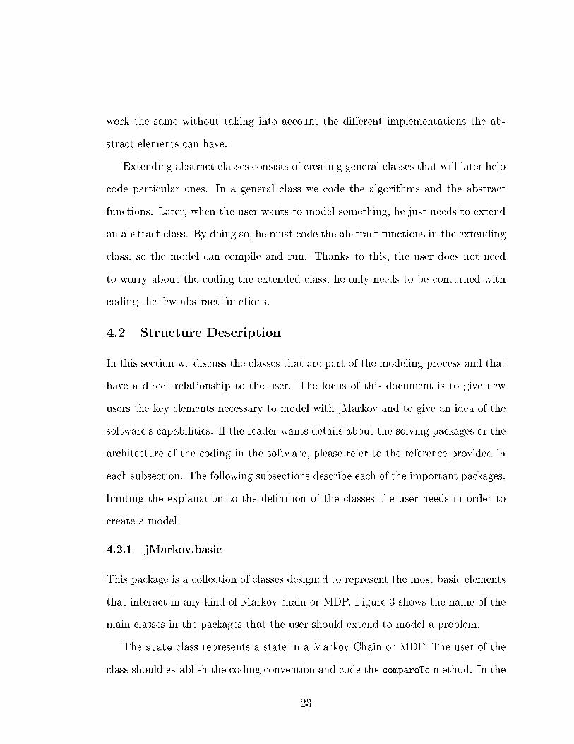
4.2.2 jMarkov and jQBD

In this package the user can �nd all the classes needed to model a Markov chain or

a QBD. Figure 4 shows two main classes: Simple MarkovProcess and GeomProcess.

For a more detailed explanation, see [45]

Figure 4: The main classes of the jMarkov modeling package

The Simple MarkovProcess class is the more general, and it is the class used to

create a CTMC or DTMC with a �nite state space. The class generates the model

through the buildRS algorithm (See Figure 5). This enables it to generate all states

and the transition matrix from the behavior rule speci�ed by the user. These rules

are determined by implementing the methods active, dests and rate.

The class GeomProcess represents a continuous or discrete QBD process. This

class extends the class Simple MarkovProcess. The building algorithm uses the in-

formation stored about the dynamics of the process to explore the graph and build

only the �rst three levels of the system. From this, extracting matrices B00, B01,

B10, A0, A1, and A2 is straightforward. Once these matrices are obtained, the sta-

bility condition is checked. If the system is found to be stable, then the matrices A0,

A1, and A2 are passed to the solver, which takes care of computing the matrix R

and the steady-state probabilities vectors π0 and π1, using the formulas described

above. The implemented solver uses the logarithmic reduction algorithm [27].

4.2.2.1 Space state building algorithm

Transitions in a CTMC are triggered by the occurrence of events such as arrivals

and departures. The matrix Q can be decomposed as Q =∑

e∈E Q(e), where Q(e)

25

contains the transition rates associated with event e, and E is the set of all possible

events that may occur.

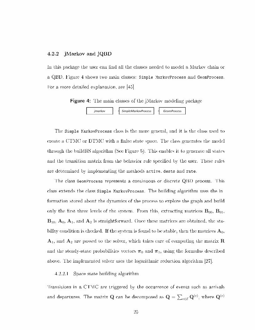
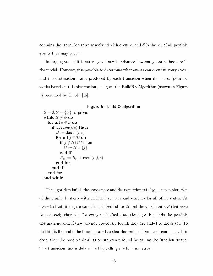
In large systems, it is not easy to know in advance how many states there are in

the model. However, it is possible to determine what events can occur in every state,

and the destination states produced by each transition when it occurs. jMarkov

works based on this observation, using an the BuildRS Algorithm (shown in Figure

5) presented by Ciardo [46].

Figure 5: BuildRS algorithm

S = ∅,U = {i0}, E given.while U 6= φ dofor all e ∈ E doif active(i, e) thenD := dests(i, e)for all j ∈ D do

if j /∈ S ∪ U then

U := U ∪ {j}end if

Rij := Rij + rate(i, j, e)end for

end if

end for

end while

The algorithm builds the state space and the transition rate by a deep exploration

of the graph. It starts with an initial state i0 and searches for all other states. At

every instant, it keeps a set of �unchecked� states U and the set of states S that have

been already checked. For every unchecked state the algorithm �nds the possible

destinations and, if they are not previously found, they are added to the U set. To

do this, it �rst calls the function active that determines if an event can occur. If it

does, then the possible destination states are found by calling the function dests.

The transition rate is determined by calling the function rate.

26

From this algorithm, we can see that a system is fully described once the states

and events are de�ned and the functions active, dests, and rate have been spec-

i�ed. As we will see, modeling a problem with jMarkov entails coding these three

functions.

4.2.2.2 User Interface

The packages of jMarkov and jQBD have a graphic interface, where the results of

the model are shown. Figure 6 shows the �rst view of the interface. Figure 7 shows

the toolbar found in the interface. Finally, �gure 8 shows a close-up of the di�erent

views of the program.

Figure 6: The User Interface of jMarkov and jQBD

Figure 7: The Toolbar

Explanation of each view:

27

Figure 8: The Interface Views

• Browse: Provides visualization of the entire system graphically. It shows the

states, events and transition probabilities in tree form.

• States: Shows all the states of the system with their respective equilibrium

probabilities.

• Rates: Shows the transition probabilities.

• MOPs: Shows the mean and the standard deviation of the system's Measures

of performance (MOP). These measures are calculated by default in some

cases, but in most the user has to code them.

• Events: Shows the system's events with the event occurrence rate as shown.

This rate indicates the expected value of occurrence of each event in a speci�c

period.

• Output: Shows a summary of all the other views, making copying and past-

ing the results in a text �le easy. Any �exible output mechanism can be

programmed from the code, bypassing the graphical interface.

4.2.3 jPhase

As explained before in section 2.4, to completely represent a continuous Phase-type

distribution (PH distribution), a user only needs the generator matrix Q and the

vector of initial probabilities or the transition probability matrix P and the vector of

28

initial probabilities for represent a discrete one. In jPhase, the user can represent the

matrix and the vector in dense or sparse form. The dense form consists of putting

the entire matrix with all its zeros. This is useful for many applications, where the

number of phases is not large and memory is not a problem. However, the sparse

form shows only the numbers di�erent from zero, so it uses a compressed sparse row.

This two types of representation are the reason why the structure of the package

shown in �gure 9 is made up of four modeling classes, the ones that the user will

usually manipulate. For further explanation of the structure of the package, refer

to [47].

Figure 9: The jPhase Main Classes

jphase

SparseContPhaseVarDenseDiscPhaseVarSparseDiscPhaseVar DenseContPhaseVar

The DenseContPhaseVar and DenseDiscPhaseVar are classes that represent con-

tinuous and discrete PH distributions with a dense representation. They have

constructors for many simple distributions, such as exponential or Erlang in the

continuous case and geometric or negative binomial in the discrete case. The

SparseContPhaseVar and SparseDiscPhaseVar classes represent continuous and dis-

crete PH distributions with a sparse representation.

4.2.3.1 jFitting

The jFitting module is a complement of jPhase and allows �tting a set of data of

a distribution to a PH distribution. Di�erent �tting algorithms can be classi�ed in

two major groups: maximum-likelihood methods and moment-matching techniques.

Some algorithms, believed to be representative of each group, are coded in di�erent

29

classes in the package and described below. For further explanation, refer to [47].

1. Moment Matching

• MomentsACPH2Fit: Implements the acyclic continuous PH distributions of

second order. This is for the continuous case [36].

• MomentsADPH2Fit: Implements the acyclic discrete PH distributions of

second order. This is for the discrete case [36].

• MomentsECCompleteFit: Erlang-Coxian distributions. The method matches

the �rst three moments of any distribution to a subclass of phase-type dis-

tributions known as Erlang-Coxian distributions. This class implements

the complete solution [37].

• MomentsECPositiveFit: Erlang-Coxian distributions. This class imple-

ments the positive solution [37].

• MomentsACPHFit: Acyclic PH distributions. The method matches the �rst

three moments of any distribution to a subclass of phase-type distribu-

tions known as acyclic phase-type distributions [38].

2. Maximum Likelihood Estimate (MLE)

• EMPhaseFit: EM for general PH distributions. The method �ts any dis-

tribution to the entire class of phase-type distributions [33].

• EMHyperExpoFit: EM for hyper-exponential distributions. The method

�ts heavy-tailed distributions to the class of hyper-exponential distribu-

tions [34].

30

• EMHyperErlangFit: EM for hyper-Erlang distributions. The method �ts

any distribution to a subclass of phase-type distributions known as hyper-

Erlang distributions [35].

4.2.3.2 Users Interface

Figure 10 shows the user interface of jPhase packages. The interface has three

important views. The �rst one shows the parameters of the PH distributions (the

matrix and the initial vectors), the other two show a graphic of the PDF and the

CDF, respectively.

Figure 10: The jPhase Interface

Figure 10 shows the user interface of jPhase packages. The interface has three

important views. The �rst one shows the parameters of the PH distributions (the

matrix and the initial vectors); the other two show a graphic of the PDF and the

CDF, respectively.

Figure 11 shows the interface for creating a new PH distribution, with examples

of the most common distributions already coded in the packages. The Figure 12

also shows the options for choosing the �tting algorithm that the user wants to use.

31

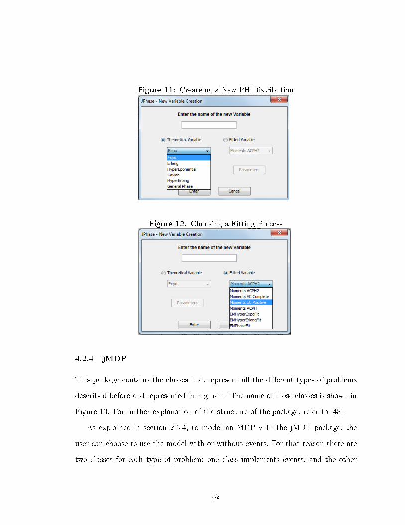
Figure 11: Createing a New PH Distribution

Figure 12: Choosing a Fitting Process

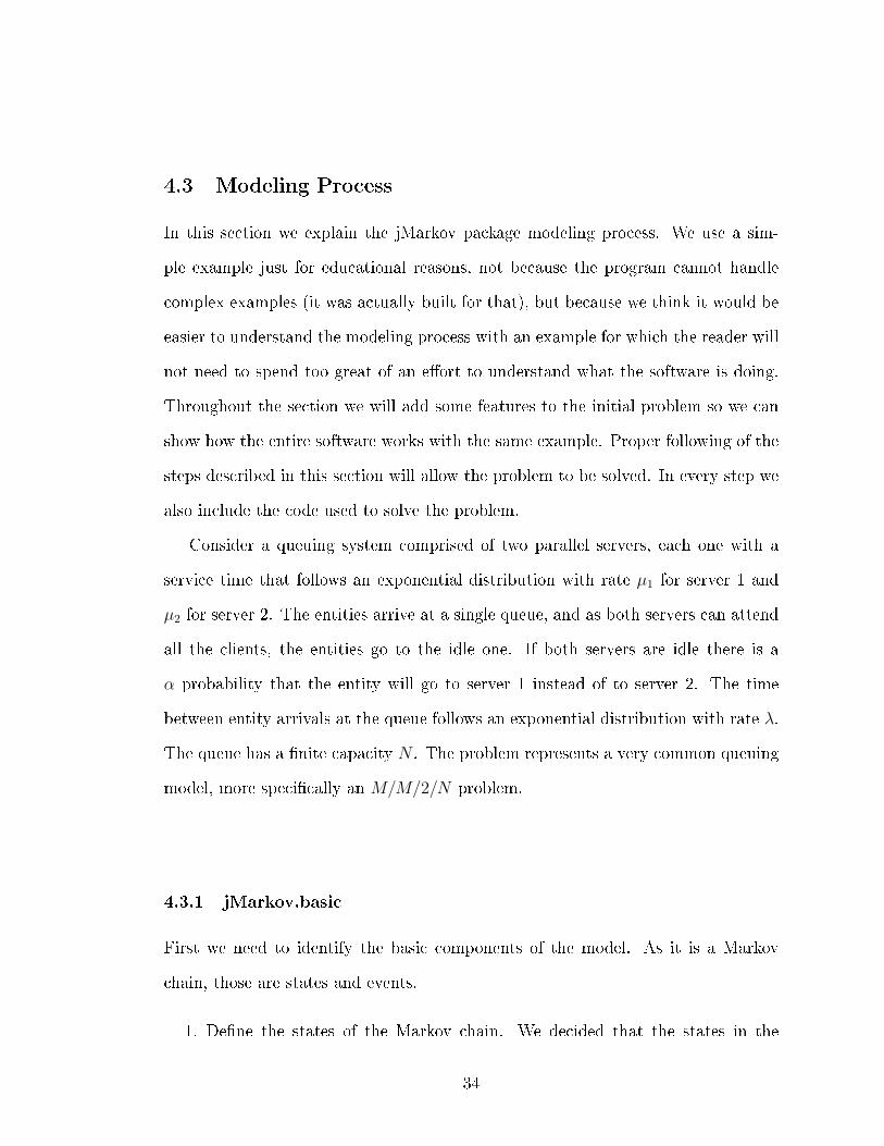
4.2.4 jMDP

This package contains the classes that represent all the di�erent types of problems

described before and represented in Figure 1. The name of those classes is shown in

Figure 13. For further explanation of the structure of the package, refer to [48].

As explained in section 2.5.4, to model an MDP with the jMDP package, the

user can choose to use the model with or without events. For that reason there are

two classes for each type of problem; one class implements events, and the other

32

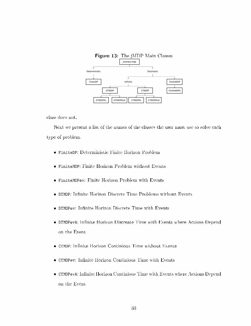
Figure 13: The jMDP Main Classes

jmarkov.mdp

DTMDP

FiniteMDPFiniteDP

FiniteMDPv

Deterministic Stochastic

Infinite

CTMDP

DTMDPEvADTMDPEv CTMDPEvACTMDPEv

class does not.

Next we present a list of the names of the classes the user must use to solve each

type of problem.

• FiniteDP: Deterministic Finite Horizon Problem

• FiniteMDP: Finite Horizon Problem without Events

• FiniteMDPev: Finite Horizon Problem with Events

• DTMDP: In�nite Horizon Discrete Time Problems without Events

• DTMDPev: In�nite Horizon Discrete Time with Events

• DTMDPevA: In�nite Horizon Discreate Time with Events where Actions Depend

on the Event

• CTMDP: In�nite Horizon Continious Time without Events

• CTMDPev: In�nite Horizon Continious Time with Events

• CTMDPevA: In�nite Horizon Continious Time with Events where Actions Depend

on the Event

33

4.3 Modeling Process

In this section we explain the jMarkov package modeling process. We use a sim-

ple example just for educational reasons, not because the program cannot handle

complex examples (it was actually built for that), but because we think it would be

easier to understand the modeling process with an example for which the reader will

not need to spend too great of an e�ort to understand what the software is doing.

Throughout the section we will add some features to the initial problem so we can

show how the entire software works with the same example. Proper following of the

steps described in this section will allow the problem to be solved. In every step we

also include the code used to solve the problem.

Consider a queuing system comprised of two parallel servers, each one with a

service time that follows an exponential distribution with rate µ1 for server 1 and

µ2 for server 2. The entities arrive at a single queue, and as both servers can attend

all the clients, the entities go to the idle one. If both servers are idle there is a

α probability that the entity will go to server 1 instead of to server 2. The time

between entity arrivals at the queue follows an exponential distribution with rate λ.

The queue has a �nite capacity N . The problem represents a very common queuing

model, more speci�cally an M/M/2/N problem.

4.3.1 jMarkov.basic

First we need to identify the basic components of the model. As it is a Markov

chain, those are states and events.

1. De�ne the states of the Markov chain. We decided that the states in the

34

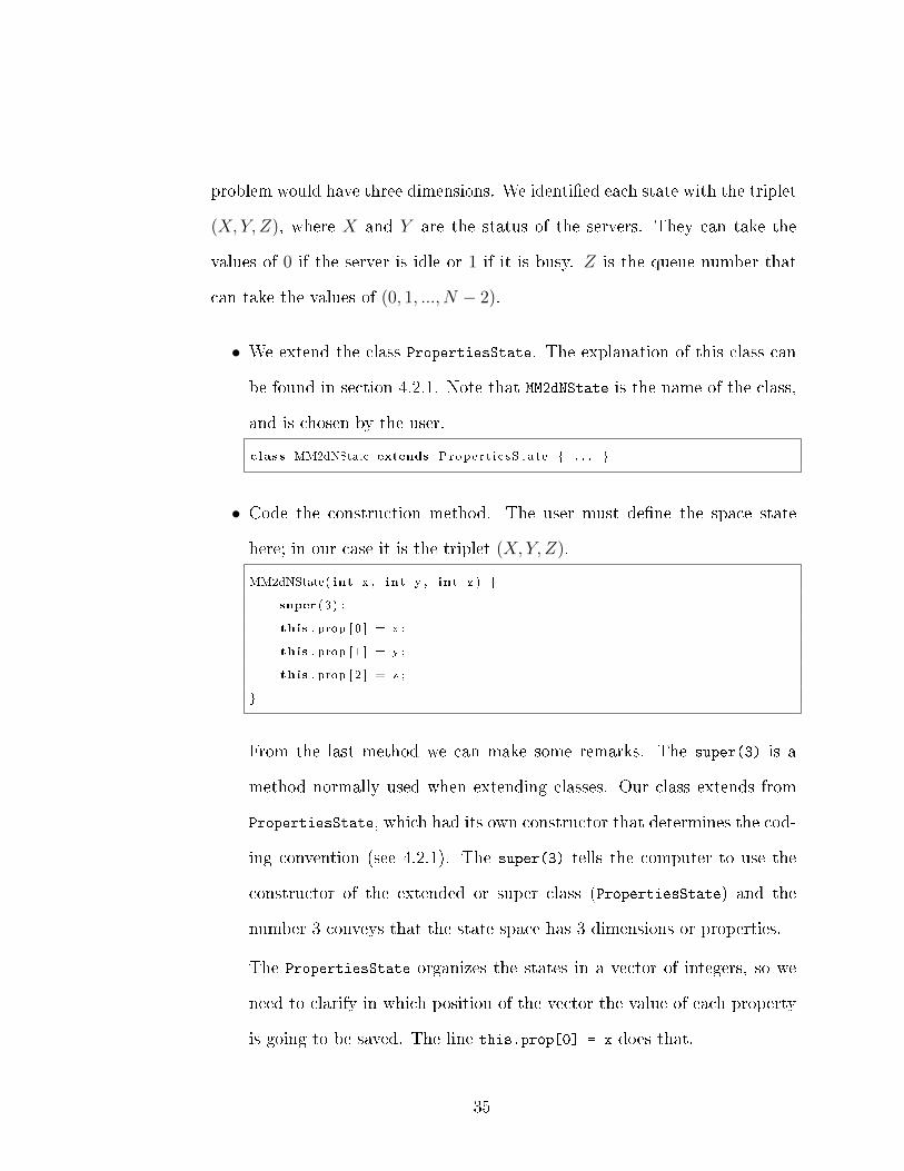
problem would have three dimensions. We identi�ed each state with the triplet

(X, Y, Z), where X and Y are the status of the servers. They can take the

values of 0 if the server is idle or 1 if it is busy. Z is the queue number that

can take the values of (0, 1, ..., N − 2).

• We extend the class PropertiesState. The explanation of this class can

be found in section 4.2.1. Note that MM2dNState is the name of the class,

and is chosen by the user.

class MM2dNState extends Prope r t i e sS t a t e { . . . }

• Code the construction method. The user must de�ne the space state

here; in our case it is the triplet (X, Y, Z).

MM2dNState( int x , int y , int z ) {

super (3 ) ;

this . prop [ 0 ] = x ;

this . prop [ 1 ] = y ;

this . prop [ 2 ] = z ;

}

From the last method we can make some remarks. The super(3) is a

method normally used when extending classes. Our class extends from

PropertiesState, which had its own constructor that determines the cod-

ing convention (see 4.2.1). The super(3) tells the computer to use the

constructor of the extended or super class (PropertiesState) and the

number 3 conveys that the state space has 3 dimensions or properties.

The PropertiesState organizes the states in a vector of integers, so we

need to clarify in which position of the vector the value of each property

is going to be saved. The line this.prop[0] = x does that.

35

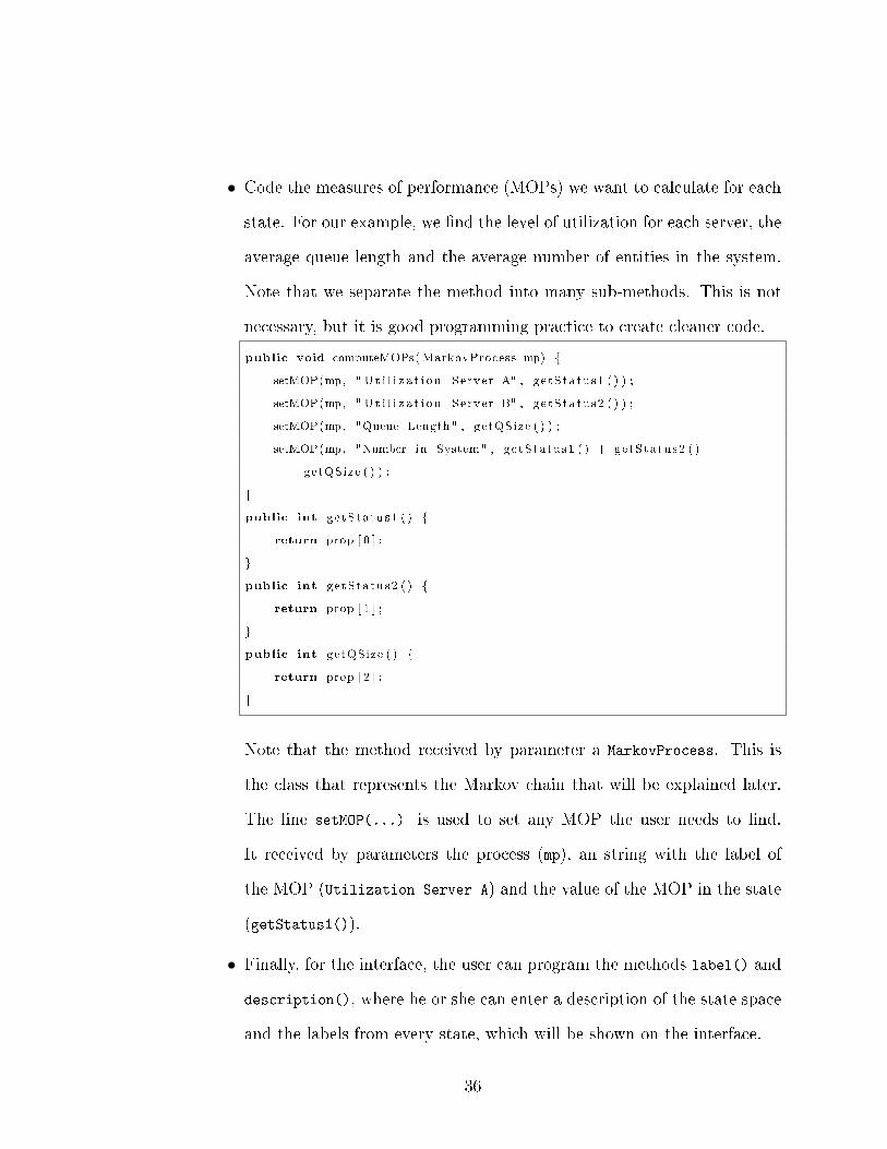
• Code the measures of performance (MOPs) we want to calculate for each

state. For our example, we �nd the level of utilization for each server, the

average queue length and the average number of entities in the system.

Note that we separate the method into many sub-methods. This is not

necessary, but it is good programming practice to create cleaner code.

public void computeMOPs(MarkovProcess mp) {

setMOP(mp, " U t i l i z a t i o n Server A" , getStatus1 ( ) ) ;

setMOP(mp, " U t i l i z a t i o n Server B" , ge tStatus2 ( ) ) ;

setMOP(mp, "Queue Length" , getQSize ( ) ) ;

setMOP(mp, "Number in System" , getStatus1 ( ) + getStatus2 ( ) +

getQSize ( ) ) ;

}

public int getStatus1 ( ) {

return prop [ 0 ] ;

}

public int getStatus2 ( ) {

return prop [ 1 ] ;

}

public int getQSize ( ) {

return prop [ 2 ] ;

}

Note that the method received by parameter a MarkovProcess. This is

the class that represents the Markov chain that will be explained later.

The line setMOP(...) is used to set any MOP the user needs to �nd.

It received by parameters the process (mp), an string with the label of

the MOP (Utilization Server A) and the value of the MOP in the state

(getStatus1()).

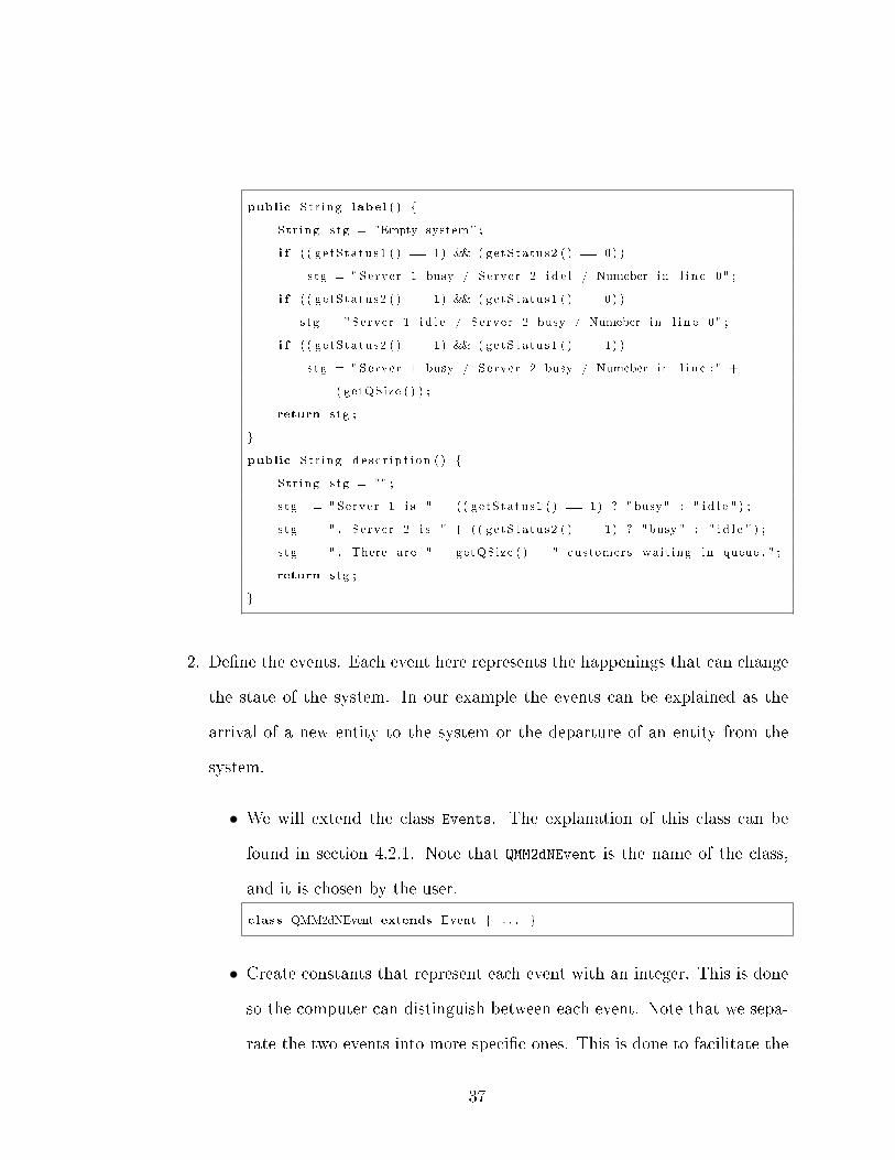
• Finally, for the interface, the user can program the methods label() and

description(), where he or she can enter a description of the state space

and the labels from every state, which will be shown on the interface.

36

public St r ing label ( ) {

St r ing s tg = "Empty system" ;

i f ( ( ge tStatus1 ( ) == 1) && ( getStatus2 ( ) == 0) )

s tg = " Server 1 busy / Server 2 i d e l / Numeber in l i n e 0" ;


s tg = " Server 1 i d l e / Server 2 busy / Numeber in l i n e 0" ;


s tg = " Server 1 busy / Server 2 busy / Numeber in l i n e : " +

( getQSize ( ) ) ;

return s tg ;

}

public St r ing d e s c r i p t i o n ( ) {

St r ing s tg = "" ;

s tg += "Server 1 i s " + ( ( getStatus1 ( ) == 1) ? "busy" : " i d l e " ) ;

s tg += " . Server 2 i s " + ( ( getStatus2 ( ) == 1) ? "busy" : " i d l e " ) ;

s tg += " . There are " + getQSize ( ) + " customers wai t ing in queue . " ;

return s tg ;

}

2. De�ne the events. Each event here represents the happenings that can change

the state of the system. In our example the events can be explained as the

arrival of a new entity to the system or the departure of an entity from the

system.

• We will extend the class Events. The explanation of this class can be

found in section 4.2.1. Note that QMM2dNEvent is the name of the class,

and it is chosen by the user.

class QMM2dNEvent extends Event { . . . }

• Create constants that represent each event with an integer. This is done

so the computer can distinguish between each event. Note that we sepa-

rate the two events into more speci�c ones. This is done to facilitate the

37

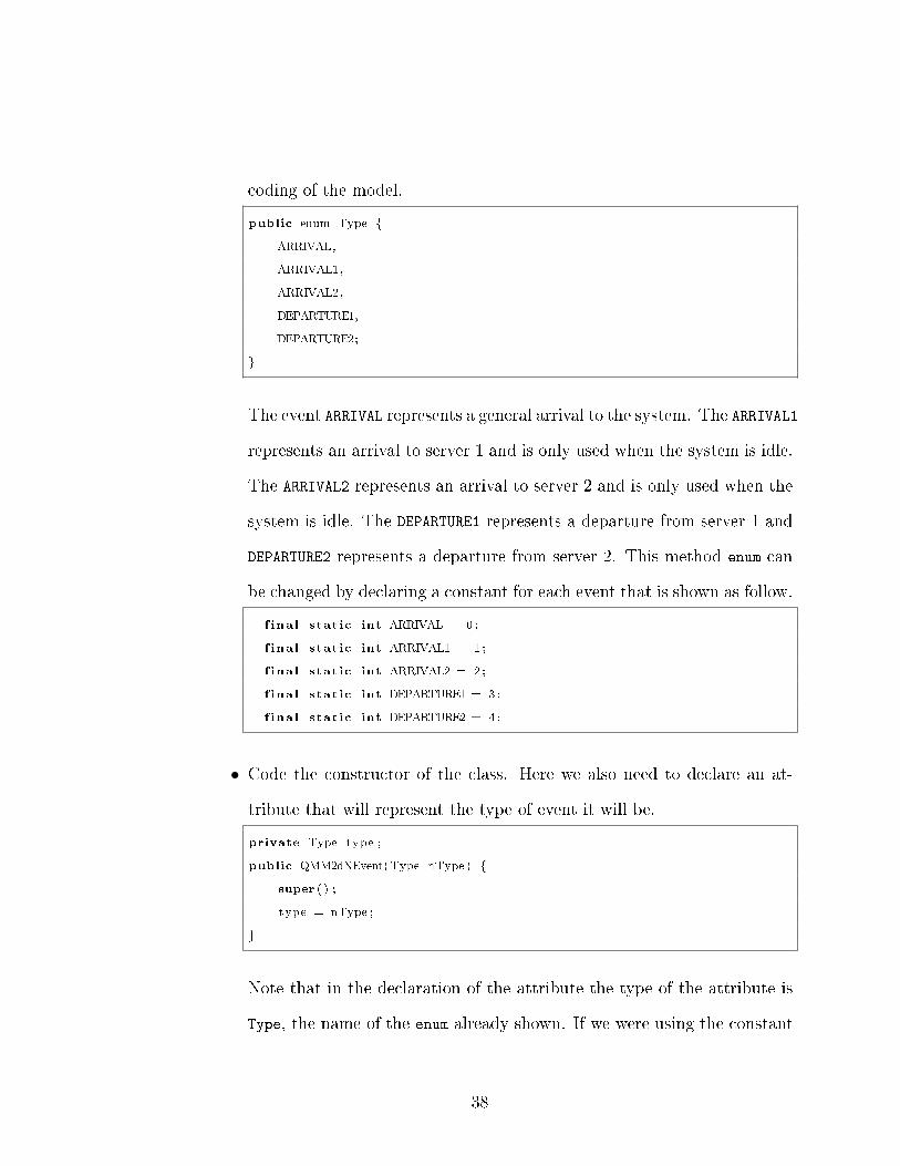
coding of the model.

public enum Type {

ARRIVAL,

ARRIVAL1,

ARRIVAL2,

DEPARTURE1,

DEPARTURE2;

}

The event ARRIVAL represents a general arrival to the system. The ARRIVAL1

represents an arrival to server 1 and is only used when the system is idle.

The ARRIVAL2 represents an arrival to server 2 and is only used when the

system is idle. The DEPARTURE1 represents a departure from server 1 and

DEPARTURE2 represents a departure from server 2. This method enum can

be changed by declaring a constant for each event that is shown as follow.

f ina l stat ic int ARRIVAL = 0 ;

f ina l stat ic int ARRIVAL1 = 1 ;

f ina l stat ic int ARRIVAL2 = 2 ;

f ina l stat ic int DEPARTURE1 = 3 ;

f ina l stat ic int DEPARTURE2 = 4 ;

• Code the constructor of the class. Here we also need to declare an at-

tribute that will represent the type of event it will be.

private Type type ;

public QMM2dNEvent(Type nType ) {

super ( ) ;

type = nType ;

}

Note that in the declaration of the attribute the type of the attribute is

Type, the name of the enum already shown. If we were using the constant

38

forms, the type of the attribute would be an integer and would look like

this: private int type;.

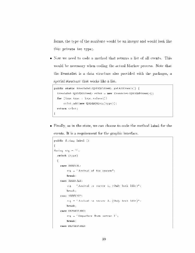
• Now we need to code a method that returns a list of all events. This

would be necessary when coding the actual Markov process. Note that

the EventsSet is a data structure also provided with the packages, a

special structure that works like a list.

public stat ic EventsSet<QMM2dNEvent> getAl lEvents ( ) {

EventsSet<QMM2dNEvent> evSet = new EventsSet<QMM2dNEvent>() ;

for (Type type : Type . va lue s ( ) )

evSet . add (new QMM2dNEvent( type ) ) ;

return evSet ;

}

• Finally, as in the state, we can choose to code the method label for the

events. It is a requirement for the graphic interface.

public St r ing label ( )

{

St r ing s tg = "" ;

switch ( type )

{

case ARRIVAL:

s tg = "Arr i va l o f the system" ;

break ;

case ARRIVAL1:

s tg = "Arr i va l to s e r v e r 1 , (Only both I d l e ) " ;

break ;

case ARRIVAL2:

s tg = "Arr i va l to s e r v e r 2 , (Only both I d l e ) " ;

break ;

case DEPARTURE1:

s tg = "Departure from se rv e r 1" ;

break ;

case DEPARTURE2:

39

s tg = "Departure from se rv e r 2" ;

break ;

}

return s tg ;

}

4.3.2 jMarkov

Now that we have coded the basic components, we are going to program the actual

process.

1. We need to extend the class that represents a �nite state Markov chain. As

shown in 4.2.2, this class name is SimpleMarkovProcess. Note that, as before,

the name of our class is QueueMM2dN and is de�ned by the user. After extending

the class we need to clarify the name of the classes that represents the state

and the event in the code. In our example the state is MM2dNState and the

event is QMM2dNEvent.

public class QueueMM2dN extends SimpleMarkovProcess<MM2dNState , QMM2dNEvent>

{ . . . }

2. We need to code the constructor of the process. We need to create an attribute

for each initial parameter, and we must initialize them in the method.

private double lambda ;

private double mu1, mu2 , alpha ;

private int N;

public QueueMM2dN(double nLambda , double nMu1, double nMu2, double nAlpha ,

int nN) {

super ( (new MM2dNState (0 , 0 , 0) ) , QMM2dNEvent . getAl lEvents ( ) ) ;

lambda = nLambda ;

mu1 = nMu1 ;

mu2 = nMu2 ;

alpha = nAlpha ;

40

N = nN;

}

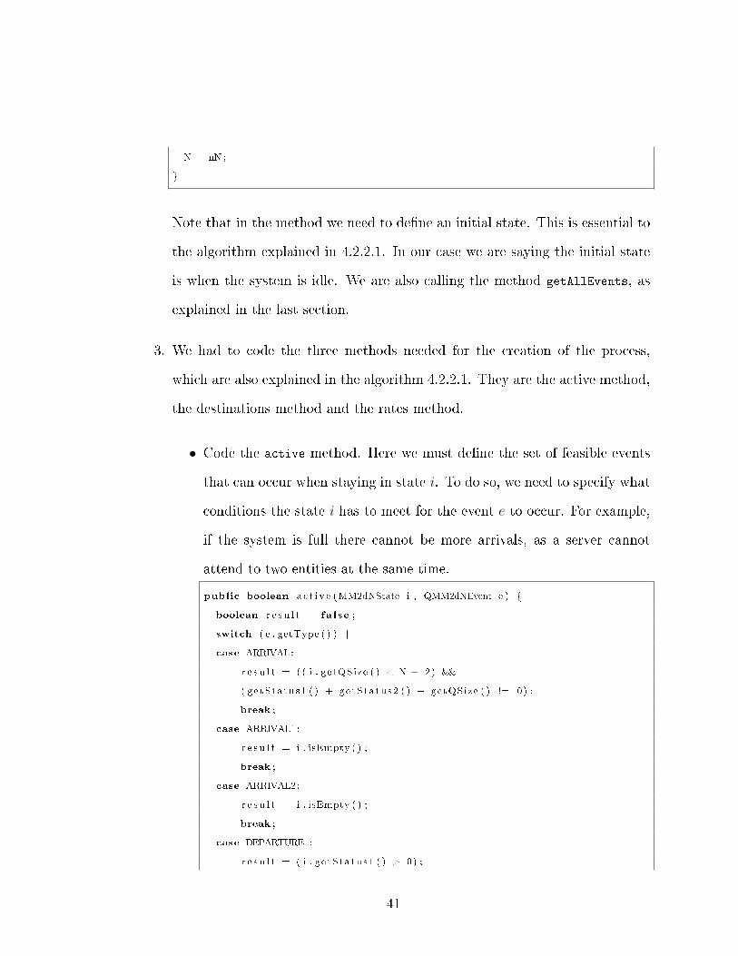
Note that in the method we need to de�ne an initial state. This is essential to

the algorithm explained in 4.2.2.1. In our case we are saying the initial state

is when the system is idle. We are also calling the method getAllEvents, as

explained in the last section.

3. We had to code the three methods needed for the creation of the process,

which are also explained in the algorithm 4.2.2.1. They are the active method,

the destinations method and the rates method.

• Code the active method. Here we must de�ne the set of feasible events

that can occur when staying in state i. To do so, we need to specify what

conditions the state i has to meet for the event e to occur. For example,

if the system is full there cannot be more arrivals, as a server cannot

attend to two entities at the same time.

public boolean a c t i v e (MM2dNState i , QMM2dNEvent e ) {

boolean r e s u l t = fa l se ;

switch ( e . getType ( ) ) {

case ARRIVAL:

r e s u l t = ( ( i . getQSize ( ) < N − 2) &&

( getStatus1 ( ) + getStatus2 ( ) + getQSize ( ) != 0) ;

break ;

case ARRIVAL1:

r e s u l t = i . isEmpty ( ) ;

break ;

case ARRIVAL2:

r e s u l t = i . isEmpty ( ) ;

break ;

case DEPARTURE1:

r e s u l t = ( i . ge tStatus1 ( ) > 0) ;

41

break ;

case DEPARTURE2:

r e s u l t = ( i . ge tStatus2 ( ) > 0) ;

break ;

}

return r e s u l t ;

}

• Code the dest method. Here the user must de�ne the set of reachable

states from state i, given that event e occurs. For our example, we need

to specify that when an arrival occurs it can be attended by an idle server

or it can go to the queue, and when a departure occurs, if there is another

in the line, it will be attended or the server will become idle. In other

words, we need to de�ne the new state j to which the system will go if it

is in state i and the event e happens.

public States<MM2dNState> de s t s (MM2dNState i , QMM2dNEvent e ) {

int newx = i . ge tStatus1 ( ) ;

int newy = i . ge tStatus2 ( ) ;

int newz = i . getQSize ( ) ;


case ARRIVAL:

i f ( i . ge tStatus1 ( ) == 0) {

newx = 1 ;

}

else i f ( i . ge tStatus2 ( ) == 0) {

newy = 1 ;

}

else {

newz = i . getQSize ( ) + 1 ;

}

break ;

case ARRIVAL1:

newx = 1 ;

break ;

42

case ARRIVAL2:

newy = 1 ;

break ;

case DEPARTURE1:

i f ( i . getQSize ( ) != 0) {

newx = 1 ;

newz = i . getQSize ( ) − 1 ;

} else {

newx = 0 ;

}

break ;

case DEPARTURE2:

i f ( i . getQSize ( ) != 0) {

newy = 1 ;

newz = i . getQSize ( ) − 1 ;

} else {

newy = 0 ;

}

break ;

}

return new StatesSet<MM2dNState>( new MM2dNState(newx , newy , newz ) ) ;

}

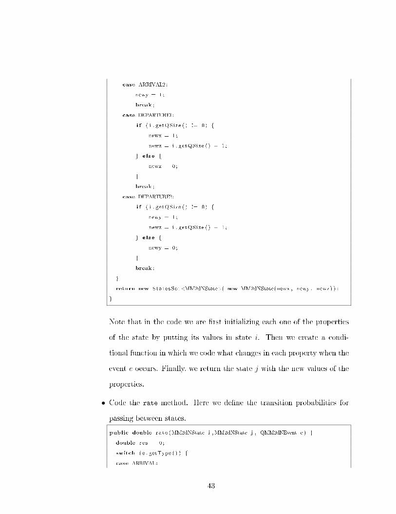
Note that in the code we are �rst initializing each one of the properties

of the state by putting its values in state i. Then we create a condi-

tional function in which we code what changes in each property when the

event e occurs. Finally, we return the state j with the new values of the

properties.

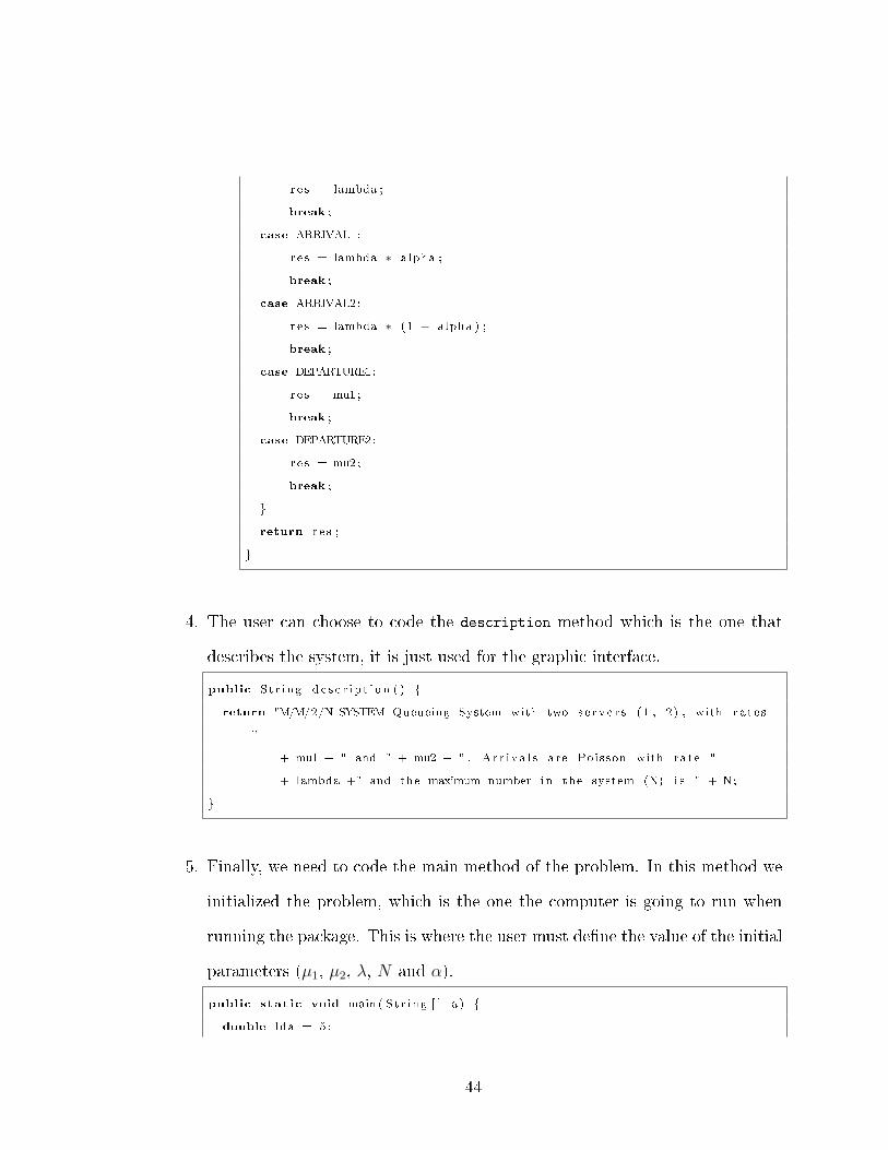
• Code the rate method. Here we de�ne the transition probabilities for

passing between states.

public double r a t e (MM2dNState i ,MM2dNState j , QMM2dNEvent e ) {

double r e s = 0 ;


case ARRIVAL:

43

r e s = lambda ;

break ;

case ARRIVAL1:

r e s = lambda ∗ alpha ;

break ;

case ARRIVAL2:

r e s = lambda ∗ (1 − alpha ) ;

break ;

case DEPARTURE1:

r e s = mu1 ;

break ;

case DEPARTURE2:

r e s = mu2 ;

break ;

}

return r e s ;

}

4. The user can choose to code the description method which is the one that

describes the system, it is just used for the graphic interface.

public St r ing d e s c r i p t i o n ( ) {

return "M/M/2/N SYSTEM Queueing System with two s e r v e r s (1 , 2) , with r a t e s

"

+ mu1 + " and " + mu2 + " . Ar r i v a l s are Poisson with ra t e "

+ lambda +" and the maximum number in the system (N) i s " + N;

}

5. Finally, we need to code the main method of the problem. In this method we

initialized the problem, which is the one the computer is going to run when

running the package. This is where the user must de�ne the value of the initial

parameters (µ1, µ2, λ, N and α).

public stat ic void main ( St r ing [ ] a ) {

double lda = 5 ;

44

double mu1 = 3 ;

double mu2 = 2

double alpha = 0 . 6 ;

int N = 10 ;

QueueMM2dN theQueue = new QueueMM2dN( lda , mu1 , mu2 , alpha , N) ;

theQueue . showGUI ( ) ;

theQueue . p r i n tA l l ( ) ;

}

4.3.2.1 Results

In this part we will show the results of the problem given by the software. We

will skip them in the following section, since our intention in showing them is to

demonstrate the utility of the software, and showing the same result format twice

would be redundant.

M/M/2/N SYSTEM

Queueing System with two s e r v e r s (1 , 2) , with r a t e s 3 .0 and 2 . 0 . A r r i v a l s are

Poisson with ra t e 5 .0 and the maximum number in the system (N) i s 10 .

System has 12 Sta t e s .

EQUILIBRUM

STATE PROBAB.

Empty system 0.04639

Server 1 i d l e / Server 2 busy / 0 l i n e 0 .05412

Server 1 busy / Server 2 i d l e / 0 l i n e 0 .04124

Server 1 busy / Server 2 busy / 0 l i n e 0 .09536









MEASURES OF PERFORMANCE

NAME MEAN SDEV

45

Ut i l i z a t i o n Server A 0.89948 0.30069

U t i l i z a t i o n Server B 0.91237 0.28275

Queue Length 3.43299 2.76915

Number in System 5.24485 3.03406

EVENTS OCCURANCE RATES

NAME MEAN RATE

Arr i va l o f the system 4.29124

Ar r i va l to s e r v e r A, (Only both I d l e ) 0 .13918

Ar r i va l to s e r v e r B, (Only both I d l e ) 0 .09278

Departure from se rv e r A 2.69845

Departure from se rv e r B 1.82474

4.3.3 jQBD

This package models in�nite Markov chains, so it is similar in many ways to the

one explained before. In that order of ideas we are just explaining the di�erences

between the coding procedures between them.

Consider the last example but with the following changes. The queue is an

in�nite one and the servers are not in parallel but in series and both cannot be busy

at the same time. In other words, until an entity has �nished the process with server

1 and then with server 2, the next entity cannot start its own process.

The basic components are still almost the same. The state class becomes the

duplet (X, Y ). We have to delete the property Z, because now the number of entities

is in�nite, so keeping track of that is impossible. The change in the event is the

deletion of the event ARRIVAL2, because now the servers are in series so the entities

always have to arrive �rst at server 1 and then at server 2. The rest of the coding

stays the same.

The di�erences are not great in the process of modeling a QBD. The methods

are the same, and the di�erences lie only in the extended class. As the queue is

46

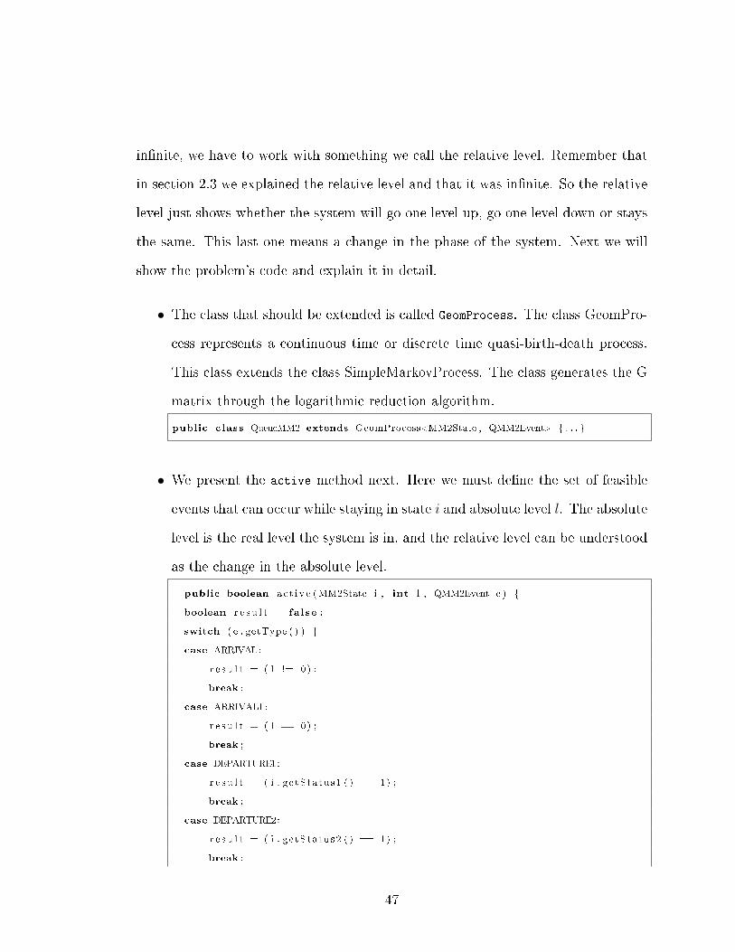
in�nite, we have to work with something we call the relative level. Remember that

in section 2.3 we explained the relative level and that it was in�nite. So the relative

level just shows whether the system will go one level up, go one level down or stays

the same. This last one means a change in the phase of the system. Next we will

show the problem's code and explain it in detail.

• The class that should be extended is called GeomProcess. The class GeomPro-

cess represents a continuous time or discrete time quasi-birth-death process.

This class extends the class SimpleMarkovProcess. The class generates the G

matrix through the logarithmic reduction algorithm.

public class QueueMM2 extends GeomProcess<MM2State , QMM2Event> { . . . }

• We present the active method next. Here we must de�ne the set of feasible

events that can occur while staying in state i and absolute level l. The absolute

level is the real level the system is in, and the relative level can be understood

as the change in the absolute level.

public boolean a c t i v e (MM2State i , int l , QMM2Event e ) {



case ARRIVAL:

r e s u l t = ( l != 0) ;

break ;

case ARRIVAL1:

r e s u l t = ( l == 0) ;

break ;

case DEPARTURE1:

r e s u l t = ( i . ge tStatus1 ( ) == 1) ;

break ;

case DEPARTURE2:

r e s u l t = ( i . ge tStatus2 ( ) == 1) ;

break ;

47

}


}

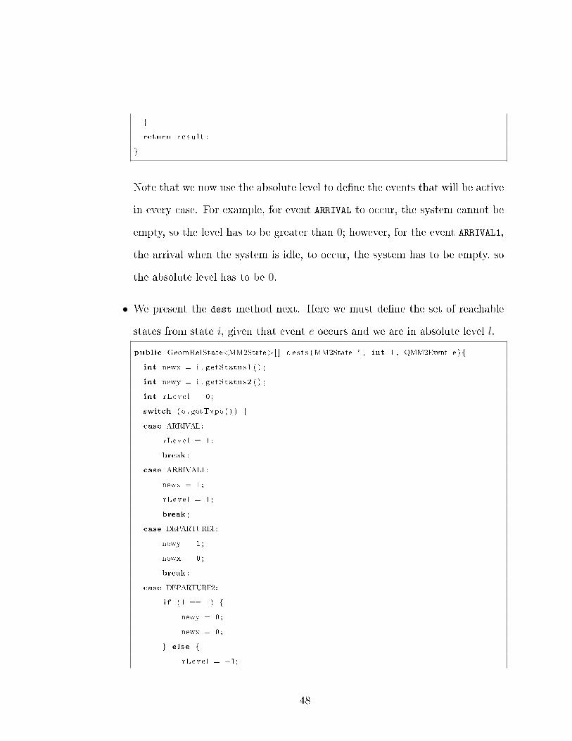
Note that we now use the absolute level to de�ne the events that will be active

in every case. For example, for event ARRIVAL to occur, the system cannot be

empty, so the level has to be greater than 0; however, for the event ARRIVAL1,

the arrival when the system is idle, to occur, the system has to be empty, so

the absolute level has to be 0.

• We present the dest method next. Here we must de�ne the set of reachable

states from state i, given that event e occurs and we are in absolute level l.

public GeomRelState<MM2State>[ ] d e s t s (MM2State i , int l , QMM2Event e ) {

int newx = i . ge tStatus1 ( ) ;

int newy = i . ge tStatus2 ( ) ;

int rLeve l = 0 ;


case ARRIVAL:

rLeve l = 1 ;

break ;

case ARRIVAL1:

newx = 1 ;

rLeve l = 1 ;

break ;

case DEPARTURE1:

newy = 1 ;

newx = 0 ;

break ;

case DEPARTURE2:

i f ( l == 1) {

newy = 0 ;

newx = 0 ;

} else {

rLeve l = −1;

48

newy = 0 ;

newx = 1 ;

}

break ;

}

MM2State newSubState = new MM2State (newx , newy) ;

GeomRelState<MM2State> s ;

i f ( e . getType ( ) == Type .DEPARTURE2 && l == 1)

{

s = new GeomRelState<MM2State> ( newSubState ) ;

} else {

s = new GeomRelState<MM2State> ( newSubState , rLeve l ) ;

}

StatesSet<GeomRelState<MM2State>> s t a t e s S e t

= new StatesSet< GeomRelState <MM2State>> ( s ) ;

return s t a t e s S e t . toStateArray ( ) ;

}

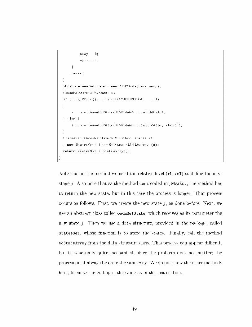
Note that in the method we used the relative level (rLevel) to de�ne the next

stage j. Also note that as the method dest coded in jMarkov, the method has

to return the new state, but in this case the process is longer. That process

occurs as follows. First, we create the new state j, as done before. Next, we

use an abstract class called GeomRelState, which receives as its parameter the

new state j. Then we use a data structure, provided in the package, called

StatesSet, whose function is to store the states. Finally, call the method

toStateArray from the data structure class. This process can appear di�cult,

but it is actually quite mechanical, since the problem does not matter; the

process must always be done the same way. We do not show the other methods

here, because the coding is the same as in the last section.

49

4.3.4 jPhase

This subsection has two parts: �rst, the jPhase package modeling explanation, and

second, how to connect this package to the last two, especially with jQBD. The

subsection is divided thus because it is important to show the entire functionality of

this package and how useful it becomes when used together with the other packages.

4.3.4.1 Modeling with jPhase

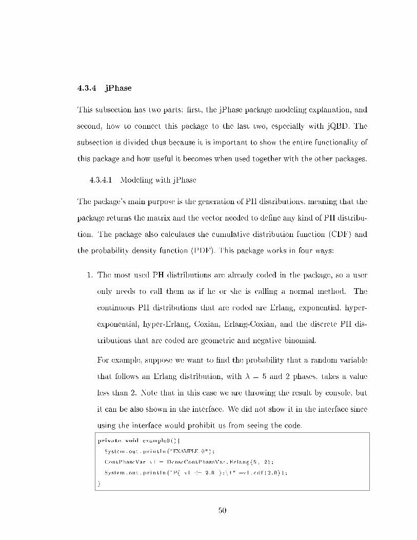
The package's main purpose is the generation of PH distributions, meaning that the

package returns the matrix and the vector needed to de�ne any kind of PH distribu-

tion. The package also calculates the cumulative distribution function (CDF) and

the probability density function (PDF). This package works in four ways:

1. The most used PH distributions are already coded in the package, so a user

only needs to call them as if he or she is calling a normal method. The

continuous PH distributions that are coded are Erlang, exponential, hyper-

exponential, hyper-Erlang, Coxian, Erlang-Coxian, and the discrete PH dis-

tributions that are coded are geometric and negative binomial.

For example, suppose we want to �nd the probability that a random variable

that follows an Erlang distribution, with λ = 5 and 2 phases, takes a value

less than 2. Note that in this case we are throwing the result by console, but

it can be also shown in the interface. We did not show it in the interface since

using the interface would prohibit us from seeing the code.

private void example0 ( ) {

System . out . p r i n t l n ( "EXAMPLE 0" ) ;

ContPhaseVar v1 = DenseContPhaseVar . Erlang (5 , 2) ;

System . out . p r i n t l n ( "P( v1 <= 2.0 ) : \ t " +v1 . cd f ( 2 . 0 ) ) ;

}

50

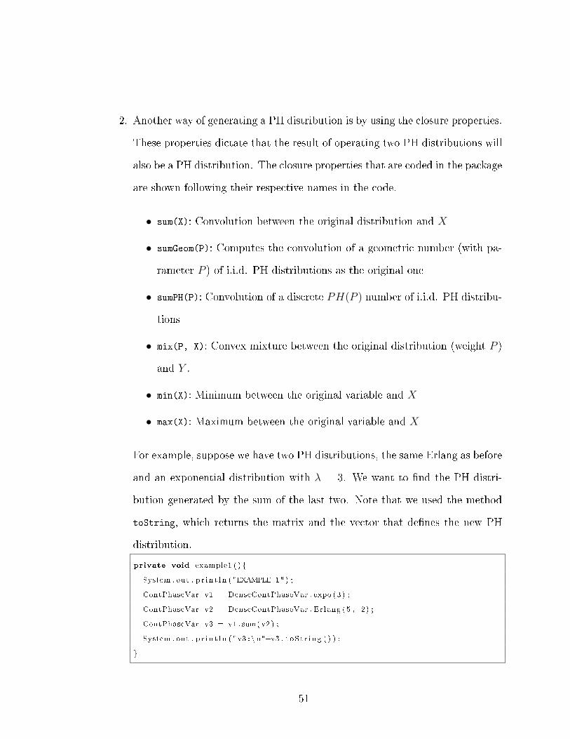
2. Another way of generating a PH distribution is by using the closure properties.

These properties dictate that the result of operating two PH distributions will

also be a PH distribution. The closure properties that are coded in the package

are shown following their respective names in the code.

• sum(X): Convolution between the original distribution and X

• sumGeom(P): Computes the convolution of a geometric number (with pa-

rameter P ) of i.i.d. PH distributions as the original one

• sumPH(P): Convolution of a discrete PH(P ) number of i.i.d. PH distribu-

tions

• mix(P, X): Convex mixture between the original distribution (weight P )

and Y .

• min(X): Minimum between the original variable and X

• max(X): Maximum between the original variable and X

For example, suppose we have two PH distributions, the same Erlang as before

and an exponential distribution with λ = 3. We want to �nd the PH distri-

bution generated by the sum of the last two. Note that we used the method

toString, which returns the matrix and the vector that de�nes the new PH

distribution.



ContPhaseVar v1 = DenseContPhaseVar . expo (3 ) ;

ContPhaseVar v2 = DenseContPhaseVar . Erlang (5 , 2) ;

ContPhaseVar v3 = v1 . sum( v2 ) ;

System . out . p r i n t l n ( "v3 : \ n"+v3 . t oS t r i ng ( ) ) ;

}

51

3. The third way consists of knowing the matrix and the vector that completely

de�ne a PH distribution. In that case, users choose the class depending on

whether the PH is continuous or discrete, and then plug in the data. Note that

we are using the classes DenseMatrix and DenseVector, and that the data can

be also supplied sparsely, using the SparseMatrixPanel class and SparseVector

class.



DenseMatrix A = new DenseMatrix (new double [ ] [ ] { {−4 ,2 ,1} , {1 ,−3 ,1} , {2 ,

1 ,−5} } ) ;

DenseVector alpha = new DenseVector (new double [ ] { 0 . 1 , 0 . 2 , 0 . 2 } ) ;

DenseContPhaseVar v1 = new DenseContPhaseVar ( alpha , A) ;

double rho = 0 . 5 ;

PhaseVar v2 = v1 . waitingQ ( rho ) ;


}

4. Finally, we can generate the PH distribution by using the jFitting module. As

previously explained, some algorithms �t a set of data or a distribution to a

PH distribution. The moment matching algorithms receive the moments of

the distribution or data to �t them, and the maximum likelihood algorithms

only receive a set of data for the �tting. If the user wants to �t a distribution

with a maximum likelihood algorithms, he or she needs to generate random

numbers that follow the distribution and use them as a set of data.

This example �ts a set of data from a plain �le with the hyper-exponential

distribution EMAlgorithm. The output of the �tting is shown under the code.



double [ ] data = readTextFi l e ( " examples / jphase /W2. txt " ) ;

52

EMHyperErlangFit f i t t e r = new EMHyperErlangFit ( data ) ;

ContPhaseVar v1 = f i t t e r . f i t (4 ) ;

i f ( v1!=null ) {


System . out . p r i n t l n ( "logLH :\ t " + f i t t e r . ge tLogLike l ihood ( ) ) ;

}

}

Phase−Type D i s t r i bu t i on

Number o f Phases : 4

Vector :

0 ,2203 0 ,4917 0 ,2054 0 ,0836

Matrix :

−0 ,1522 0 ,0000 0 ,0000 0 ,0000

0 ,0000 −0 ,9164 0 ,0000 0 ,0000

0 ,0000 0 ,0000 −9 ,1779 0 ,0000

0 ,0000 0 ,0000 0 ,0000 −233 ,1610

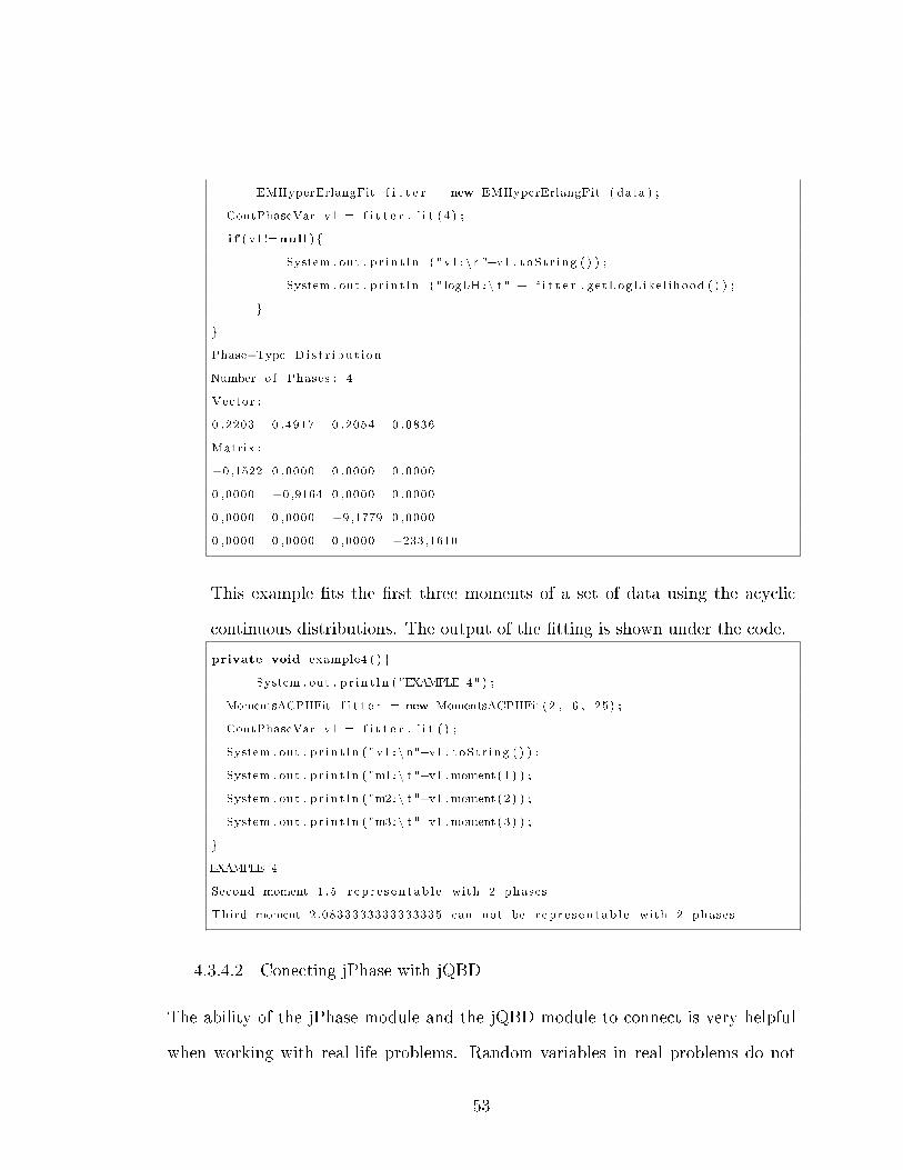
This example �ts the �rst three moments of a set of data using the acyclic

continuous distributions. The output of the �tting is shown under the code.



MomentsACPHFit f i t t e r = new MomentsACPHFit (2 , 6 , 25) ;

ContPhaseVar v1 = f i t t e r . f i t ( ) ;


System . out . p r i n t l n ( "m1: \ t "+v1 .moment (1 ) ) ;



}

EXAMPLE 4

Second moment 1 .5 r ep r e s en t ab l e with 2 phases

Third moment 2.0833333333333335 can not be r ep r e s en t ab l e with 2 phases

4.3.4.2 Conecting jPhase with jQBD

The ability of the jPhase module and the jQBD module to connect is very helpful

when working with real-life problems. Random variables in real problems do not

53

normally follow an exponential distribution, so the ability of the jPhase and the

jQBD to combine is a powerful tool when modeling real life problems.

A PH distribution can be modeled with jQBD without the need of jPhase, how-

ever it would be much easier to use them together. The example in section 4.3.3

can be seen as a QBD with a PH distribution. Let us imagine that there are not

two servers, but rather just one server, and the entities have to follow two phases of

service to complete the process. Then we will have an M/PH/1 queue. But work-

ing with just jQBD can be complicated when handling large PH distributions with

many phases. For that reason, working with the two packages together is easier and

very important.

Going back to our example, consider the same system with one queue, but instead

of two servers we have only one, which has a hyper-exponential service time. Let us

suppose the arrivals are also hyper-exponentials.

As always, we must start by coding the basic components. The state space X

would be de�ned as the current phase of the service (1, ..., N) or 0 if the system is

idle, and the events would be just two, an arrival or a departure from the system.

We will skip the coding of these two because it is identical to that explained in the

previous sections.

Then we have to code the QBD process. We just paste the active, dest and

rate methods to show how the packages can connect. We skip the other methods

because they do not present a signi�cant change.

1. Active Method.

public boolean a c t i v e ( HiperExQueueState i , int iLeve l , HiperExQueueEvent e ) {


switch ( e . type ) {

case ARRIVAL:

54

r e s u l t = true ;

break ;

case FINISH_SERVICE :

r e s u l t = ( i . getSrvPhase ( ) == e . getCurPH ( ) ) ;

break ;

}


}

Note that the getSrvPhase asks for the current service phase of state i, but the

getCurPH is asking for the total phases of the hyper-exponential distribution

we are modeling. The ARRIVAL returns true because it is always active, and

the queue in QBD is in�nite.

2. Dests Method.

public GeomRelState<HiperExQueueState >[ ] d e s t s ( HiperExQueueState i ,

int absLevel , HiperExQueueEvent e ) {

Sta t e sSe t <GeomRelState <HiperExQueueState>> de s tS ta t e s

= new Sta t e sSe t <GeomRelState <HiperExQueueState>>() ;

int newPhase = i . getSrvPhase ( ) ;

int rLeve l = 0 ;


case ARRIVAL:

rLeve l = +1;

i f ( absLeve l == 0)

addDestsFin i shServer ( rLevel , d e s tS t a t e s ) ;

else

de s tS ta t e s . add (new GeomRelState <HiperExQueueState>(

new HiperExQueueState ( newPhase ) , rLeve l ) ) ;

break ;


rLeve l = −1;

i f ( absLeve l == 1)

de s tS ta t e s . add (new GeomRelState <HiperExQueueState>

(new HiperExQueueState (0 ) ) ) ;

55

else

addDestsFin i shServer ( rLevel , d e s tS t a t e s ) ;

break ;

}

return de s tS ta t e s . toStateArray ( ) ;

3. Rate Method.

public double r a t e ( HiperExQueueState i , int iLeve l , HiperExQueueState j , int

jLeve l ,

HiperExQueueEvent e ) {

double r a t e = −1;

double [ ] a = se rvD i s t . getMat0Array ( ) ;


case ARRIVAL:

i f ( i L ev e l == 0) {

int newPhase = j . getSrvPhase ( ) ;

double alpha [ ] = se rvD i s t . getVectorArray ( ) ;

r a t e = lambda ∗ alpha [ newPhase − 1 ] ;

}

else {

ra t e = lambda ;

}

break ;


i f ( i L ev e l > 1) {

int newPhase = j . getSrvPhase ( ) ;

double alpha [ ] = se rvD i s t . getVectorArray ( ) ;

r a t e = a [ e . getCurPH ( ) − 1 ] ∗ alpha [ newPhase − 1 ] ;

}

else {

ra t e = a [ e . getCurPH ( ) − 1 ] ;

}

break ;

}

return r a t e ;

56

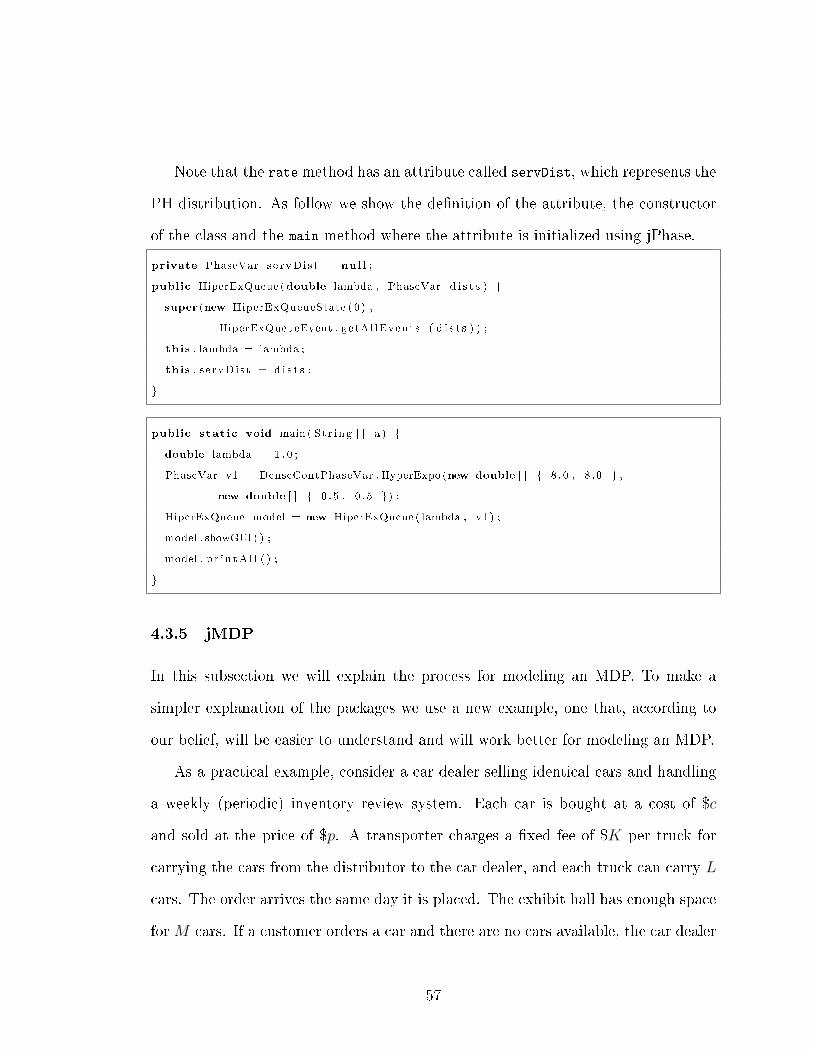
Note that the ratemethod has an attribute called servDist, which represents the

PH distribution. As follow we show the de�nition of the attribute, the constructor

of the class and the main method where the attribute is initialized using jPhase.

private PhaseVar s e rvD i s t = null ;

public HiperExQueue (double lambda , PhaseVar d i s t s ) {

super (new HiperExQueueState (0 ) ,

HiperExQueueEvent . getAl lEvents ( d i s t s ) ) ;

this . lambda = lambda ;

this . s e rvD i s t = d i s t s ;

}

public stat ic void main ( St r ing [ ] a ) {

double lambda = 1 . 0 ;

PhaseVar v1 = DenseContPhaseVar . HyperExpo (new double [ ] { 8 . 0 , 8 . 0 } ,

new double [ ] { 0 . 5 , 0 . 5 }) ;

HiperExQueue model = new HiperExQueue ( lambda , v1 ) ;

model . showGUI ( ) ;

model . p r i n tA l l ( ) ;

}

4.3.5 jMDP

In this subsection we will explain the process for modeling an MDP. To make a

simpler explanation of the packages we use a new example, one that, according to

our belief, will be easier to understand and will work better for modeling an MDP.

As a practical example, consider a car dealer selling identical cars and handling

a weekly (periodic) inventory review system. Each car is bought at a cost of $c

and sold at the price of $p. A transporter charges a �xed fee of $K per truck for

carrying the cars from the distributor to the car dealer, and each truck can carry L

cars. The order arrives the same day it is placed. The exhibit hall has enough space

for M cars. If a customer orders a car and there are no cars available, the car dealer

57

gives him the car as soon as it arrives with a $b discount. The car dealer does not

allow more than B backorders of this type. Holding inventory implies a capital cost

of β annually (in the form of interest rate). The marketing data indicates that the

demand follows a Poisson distribution with a mean of θ cars per week. The dealer

is looking for an optimal ordering policy that minimizes its costs. The rest of this

section describes the detailed modeling process. [48]

Let Dt represent the random weekly demand, pn = P{Dt = n} and qn = P{Dt ≥

n}. The problem is an in�nite-horizon stochastic decision-making problem. It is

possible to model the problem with or without events.

In order to solve the problem, the following steps are to be completed. In every

step we include the code used to solve the problem. For this problem the stages are

de�ned as weeks because, as stated earlier, the inventory review happens weekly.

The modeling process is:

1. De�ne the states of the Markov chain. For our example, each state is the level

of physical inventory (Xt) at the end of week t. The class InvLevel represents

each state.

public class InvLeve l extends StateArray {

public InvLeve l ( int k ) {

super (new int [ ] {k}) ;

}

public int getLeve l ( ) {

return s t a tu s [ 0 ] ;

}


return "Leve l " + getLeve l ( ) ;

}

}

58

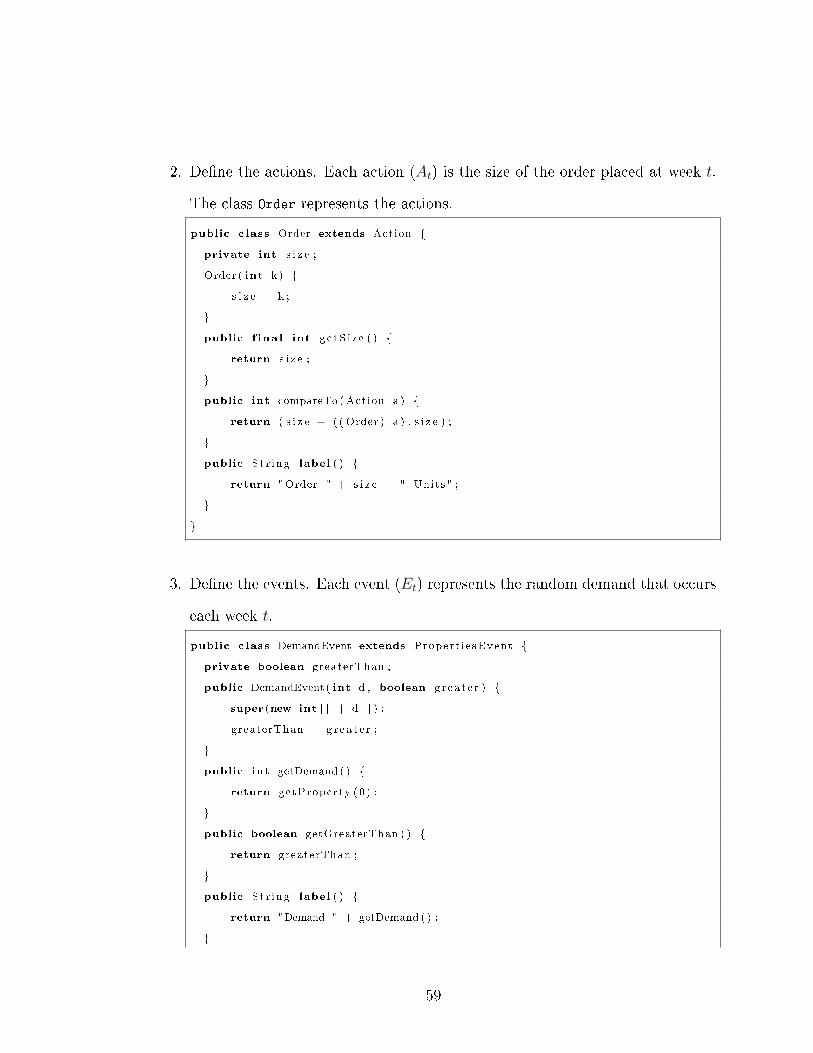
2. De�ne the actions. Each action (At) is the size of the order placed at week t.

The class Order represents the actions.

public class Order extends Action {

private int s i z e ;

Order ( int k ) {

s i z e = k ;

}

public f ina l int g e tS i z e ( ) {

return s i z e ;

}

public int compareTo ( Action a ) {

return ( s i z e − ( ( Order ) a ) . s i z e ) ;

}


return "Order " + s i z e + " Units " ;

}

}

3. De�ne the events. Each event (Et) represents the random demand that occurs

each week t.

public class DemandEvent extends Propert i e sEvent {

private boolean greaterThan ;

public DemandEvent ( int d , boolean g r e a t e r ) {

super (new int [ ] { d }) ;

greaterThan = gr ea t e r ;

}

public int getDemand ( ) {

return getProperty (0 ) ;

}

public boolean getGreaterThan ( ) {

return greaterThan ;

}


return "Demand " + getDemand ( ) ;

}

59

}

4. Select the type of problem. The problem is an in�nite-horizon problem. It is

stochastic and the time is discrete. We will use events; therefore, we should

extend the class DTMDPEv. After extending the class, we need to clarify the

name of the classes that represent the state, action and event in the code. In

our example, InvLevel is the state, Order is the action and DemandEvent is the

event.

public class ControlProduccion extends DTMDPEv<InvLevel , Order , DemandEvent>

{ . . . }

5. De�ne the set of feasible actions from state i. For each state i the feasible

actions that can be taken are those that will not exceed the exhibit hall's

capacity. The maximum order feasible is M − i, so the feasible set of actions

for each state i is A(i) = {0, . . . ,M − i}.

public Actions<Order> f e a s i b l eA c t i o n s ( InvLeve l i ) {

ActionsSet<Order> ac t i onSe t = new ActionsSet<Order >() ; //empty s e t

int max = maxInventory − i . g e tLeve l ( ) ;

for ( int n = 0 ; n <= max ; n++){

ac t i onSe t . add (new Order (n) ) ; //add each f e a s i b l e ac t ion

}

return ac t i onSe t ; // return the s e t

}

6. De�ne the set of active events. For each state i and given that action a is

taken, we de�ne the feasible events that can occur. For example, zero-demand

is active in every state. Demand equal to i + a + B is indistinguishable from

larger demands. So the sets of active events are E(i, a) = {0, . . . , i+ a+B}.

60

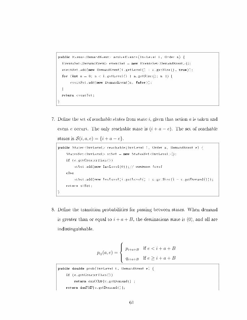
public Events<DemandEvent> act iveEvents ( InvLeve l i , Order a ) {

EventsSet<DemandEvent> eventSet = new EventsSet<DemandEvent>() ;

eventSet . add (new DemandEvent ( i . ge tLeve l ( ) + a . g e tS i z e ( ) , true ) ) ;

for ( int n = 0 ; n < i . ge tLeve l ( ) + a . g e tS i z e ( ) ; n++) {

eventSet . add (new DemandEvent (n , fa l se ) ) ;

}

return eventSet ;

}

7. De�ne the set of reachable states from state i, given that action a is taken and

event e occurs. The only reachable state is (i + a − e). The set of reachable

states is S(i, a, e) = {i+ a− e}.

public States<InvLevel> reachab l e ( InvLeve l i , Order a , DemandEvent e ) {

StatesSet<InvLevel> s tSe t = new StatesSet<InvLevel >() ;

i f ( e . getGreaterThan ( ) )

s tS e t . add (new InvLeve l (0 ) ) ; // minimum l e v e l

else

s tS e t . add (new InvLeve l ( i . g e tLeve l ( ) + a . g e tS i z e ( ) − e . getDemand ( ) ) ) ;

return s tS e t ;

}

8. De�ne the transition probabilities for passing between states. When demand

is greater than or equal to i+ a+B, the destinations state is (0), and all are

indistinguishable.

pij(a, e) =

pi+a+B if e < i+ a+B

qi+a+B if e ≥ i+ a+B

public double prob ( InvLeve l i , DemandEvent e ) {

i f ( e . getGreaterThan ( ) )

return demCCDF[ e . getDemand ( ) ] ;

return demPMF[ e . getDemand ( ) ] ;

61

}

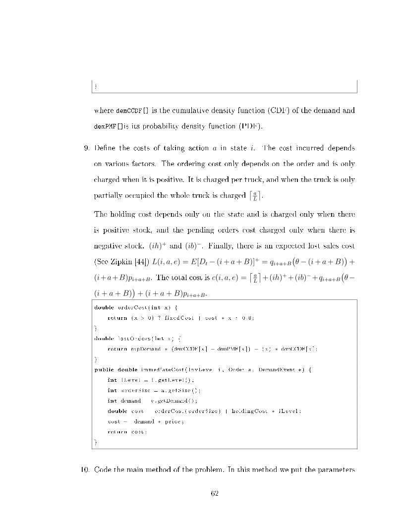
where demCCDF[] is the cumulative density function (CDF) of the demand and

demPMF[]is its probability density function (PDF).

9. De�ne the costs of taking action a in state i. The cost incurred depends

on various factors. The ordering cost only depends on the order and is only

charged when it is positive. It is charged per truck, and when the truck is only

partially occupied the whole truck is charged⌈aL

⌉.

The holding cost depends only on the state and is charged only when there

is positive stock, and the pending orders cost charged only when there is

negative stock. (ih)+ and (ib)−. Finally, there is an expected lost sales cost

(See Zipkin [44]) L(i, a, e) = E[Dt− (i+ a+B)]+ = qi+a+B(θ− (i+ a+B)

)+

(i+a+B)pi+a+B. The total cost is c(i, a, e) =⌈aL

⌉+(ih)++(ib)−+qi+a+B

(θ−

(i+ a+B))+ (i+ a+B)pi+a+B.

double orderCost ( int x ) {

return ( x > 0) ? f ixedCost + cos t ∗ x : 0 . 0 ;

}

double l o s tOrde r s ( int x ) {

return expDemand ∗ (demCCDF[ x ] − demPMF[ x ] ) − ( x ) ∗ demCCDF[ x ] ;

}

public double immediateCost ( InvLeve l i , Order a , DemandEvent e ) {

int i L ev e l = i . ge tLeve l ( ) ;

int o rde rS i z e = a . g e tS i z e ( ) ;

int demand = e . getDemand ( ) ;

double co s t = orderCost ( o rd e rS i z e ) + hold ingCost ∗ i L ev e l ;

c o s t −= demand ∗ p r i c e ;

return co s t ;

}

10. Code the main method of the problem. In this method we put the parameters

62

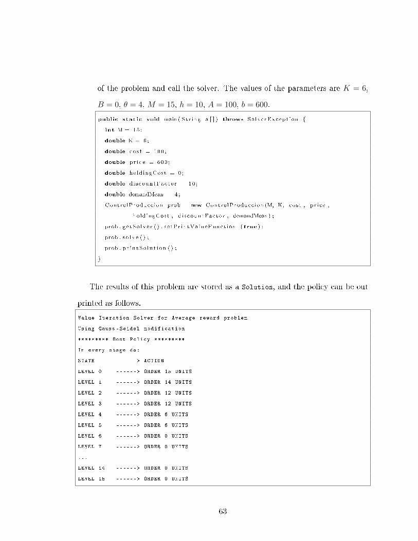
of the problem and call the solver. The values of the parameters are K = 6,

B = 0, θ = 4, M = 15, h = 10, A = 100, b = 600.

public stat ic void main ( St r ing a [ ] ) throws SolverExcept ion {

int M = 15 ;

double K = 6 ;

double co s t = 100 ;

double p r i c e = 600 ;

double hold ingCost = 0 ;

double di scountFactor = 10 ;

double demandMean = 4 ;

ControlProduccion prob = new ControlProduccion (M, K, cost , p r i c e ,

holdingCost , d i scountFactor , demandMean) ;

prob . g e tSo l v e r ( ) . se tPr intValueFunct ion ( true ) ;

prob . s o l v e ( ) ;

prob . p r i n tSo l u t i on ( ) ;

}

The results of this problem are stored as a Solution, and the policy can be out

printed as follows.

Value Iteration Solver for Average reward problem

Using Gauss -Seidel modification

********* Best Policy *********

In every stage do:

STATE ------> ACTION

LEVEL 0 ------> ORDER 15 UNITS








...



63

Chapter V

Applications in Real Life Problems

In this section we will enumerate some of the work done with the jMarkov software

by di�erent students for their thesis projects, giving only a very brief summary of

their work. We also provide references for interested readers who want to �nd out

more about these projects.

• Blocking models on inventory analysis: The author studied an order picking

system. One of the biggest problems in those systems was the blocking in

the trajectory of the workers while picking the products. The workers' idle

time was translated in delivery delays and additional expenses. The idea

of the project was to minimize this idle time using jMakov and simulation

techniques [49].

• A dynamic programming model for structuring mortgage-backed securities:

The project was based on the structure of the Colombian mortgage securities

issued in the Colombian stock market. The author used dynamic program-

ming for restructuring the securities, lowering their issued cost through the

minimization of the future payments to the bondholders. This paper won the

best paper award in the IEEE SIEDS 2005 [50].

64

• Implementation of the shortest path: the project intended to built a generic

algorithm to solve stochastic shortest-path problems using the jMarkov soft-

ware [51].

• A parallel partitioned e�cient-value iteration: The idea of the project was

to create an extension of the jMarkov software, explicitly in the jMDP pack-

age. The author achieved more e�cient results while running the solution

algorithms by using clusters of computers for the calculations [52].

• Linear programming solvers for Markov decision processes: The project con-

nected the jMarkov software to some of the most commercial linear program-

ming optimization software's. The author gave more �exibility to the jMarkov

software so the users could solve Markov decision process through linear pro-

gramming [53].

65

Chapter VI

Conclusions

The jMarkov package was coded with the objective of creating a user-friendly envi-

ronment. We concentrated all our e�orts to create a software program that allows

the user to model any kind of system, like an Markov chain, a QBD or an MDP,

with fairly basic knowledge of programming. To this end, we separated the modeling

part from the solution algorithms. Therefore, the user only needs to mathematically

model the problem as explained in the previous sections and the software will solve

the problem.

Although jMarkov is a user-friendly software, the existing documentation ex-

plaining how it works is not. Any kind of software needs explanatory documentation

to explain it, which must be written for every type of reader. This is the reason we

present a user manual that explains the basic principles for modeling with jMarkov.

The user manual is divided into three sections, namely: programming knowledge,

structure description and modeling process. The programming knowledge section

gives the basic programming components needed to understand and model with

jMarkov. We de�ne the abstraction capabilities of Java.

In the structure description we explain the main components of the software that

the user must know about. These include the basic elements package, the jMarkov

66

package, the jQBD package, the jPhase package and the jMDP package. The �rst

collects all the basic components a stochastic problem should have and which are

essential for its modeling; here we have a class that represents a state or an event.

The other ones are used to model Markov chains, quasi-birth-death processes, phase-

type distributions and Markov decision processes, respectively. They have all the

classes that represent every type of problem we have discussed previously in the

document. Those classes are the ones in charge of modeling the system based on

what the user codes.

In this part we successfully decrease the number of classes the user must work

with in each component. The basic elements package contains 24 classes, but we

determine that only 6 are important. jMarkov and jQBD have 6 classes, narrowed

down to 2. jPhase has 18 classes, but only 4 are essential. Finally, jMDP has 13

classes, of which 8 are important.

We explain the modeling process for stochastic problems in our software by using

practical examples and giving a list of real-life problems that have been solved using

jMarkov to show the full capacity of the software. In conclusion, we have created a

user-friendly manual that any type of person can use to learn to work with jMarkov,

making the software an easy-to use tool.

67

References

[1] Java Developers Site, Sun Microsystems. http://sun.java.com

[2] A. Riska and E. Smirni. MAMSolver: A matrix analytic methods tool. In Pro-

ceedings of the 12-th international conference on modeling Techniques and tools

for computer and communication system performance evaluation tools, pages

205-211, April 2002.

[3] B. R. Haverkort, A. P. van Moorsel, and A. Dijkstra. MGMtool: A performance

modelling tool based on matrix geometric techniques. In R. Pooley and J. Hill-

ston, editors, Computer performance evaluation '92, modelling techniques and

tools, pages 397-401. Antony Rowe Ltd., 1992.

[4] S. Li, S. Park, and D. Ari�er. SMAQ: Ameasurement-based tool for tra�c

modeling and queuing analysis Part I: Design methodologies and software ar-

chitecture. IEEE Communications Magazine, 36:56-65, August 1998.

[5] D. Potier and M. Veran. QNAP2: A portable environment for queueing sys-

tems modelling. In Modelling and Tools for Performance Analysis. Proceedings

of the First International Conference on Modelling Techniques and Tools for

Computer Performance Evaluation, 1984.

68

http://sun.java.com

http://sun.java.com

[6] W. J. Stewart. Introduction to the Numerical Solution of Markov Chains, vol-

ume First edition. Princeton University Press, 1994.

[7] O.J. Dahl and K. Nygaard. SIMULA - an ALGOL-based simulation language.

Communications of the ACM, 9(9):671-678, September 1966.

[8] William J. Stewart. MARCA: Markov chain analyzer, a software package for

markov modelling. Technical report, North Carolina State University - Depart-

ment of Computer Science, 1996.

[9] G. Ciardo, R. Jones, A. Miner, and R. Siminiceanu. SMART: Stochastic Model-

checking Analyzer for Reliability and Timing. In Proceedings of the Interna-

tional Conference on Dependable Systems and Networks (DSN'02), 2002.

[10] Christel Baier, Frank Ciesinski, and Marcus Groÿer. PROBMELA: a modeling

language for communicating probabilistic processes. University at Bonn,Institut

for Informatik I, Germany,.

[11] W. Knottenbelt. Generalised markovian analysis of timed transitions systems.

Master's thesis, Department of Computer Science, Faculty of Science, Univer-

sity of Cape Town, June 1996.

[12] Alan Dormer, Alkis Vazacopoulos, Nitin Verma, and Horia Tipi. Modeling and

solving stochastic programming problems in supply chain management using

Xpress-SP. Dash Optimization, Inc.

[13] AMPL. Stochastic programming extensions proposed new AMPL features.

Technical report, AMPL http://www.ampl.com/NEW/FUTURE/stoch.html,

August1996

69

http://www.ampl.com/NEW/FUTURE/stoch.html, August 1996




[14] Patrick Valente. SAMPL/SPInE user's manual. Technical report, OptiRisk Sys-

tems, Middlesex, United Kingdom, 2002.

[15] Yih-Long Chang and Kiran Desai. WinQSB, Version 2.0. John Wiley and Sons,

2003.

[16] Bernard Lamond. An interactive computer program for markov dynamic pro-

gramming. Technical report, Universite Laval Department doperations et sys-

temes de decision, October 1984.

[17] Markov Decision Processes (MDP) Toolbox http://www.inra.fr/internet/

Departements/MIA/T//MDPtoolbox/

[18] Poupart, Pascal. Symbolic Perseus. http://www.cs.uwaterloo.ca/

~ppoupart/

[19] Smith, Trey. ZMDP Software for POMDP and MDP Planning. http://www.

cs.cmu.edu/~trey/zmdp/

[20] Cassandra, Anthony. POMDP solver software. http://www.cs.brown.edu/

research/ai/pomdp/

[21] Spaan, Matthijs. Perseus. http://staff.science.uva.nl/~mtjspaan/

software/approx/

[22] Taha, Tarek. POMDP Tools. http://www.tarektaha.com/research/

download.php?list.3

[23] Caylus open source library for MDP. http://sourceforge.net/projects/

caylus/

70

hhttp://www.inra.fr/internet/Departements/MIA/T//MDPtoolbox/

http://www.inra.fr/internet/Departements/MIA/T//MDPtoolbox/

hhttp://www.inra.fr/internet/Departements/MIA/T//MDPtoolbox/

http://www.inra.fr/internet/Departements/MIA/T//MDPtoolbox/

http://www.cs.uwaterloo.ca/~ppoupart/




http://www.cs.cmu.edu/~trey/zmdp/




http://www.cs.brown.edu/research/ai/pomdp/




http://staff.science.uva.nl/~mtjspaan/software/approx/




http://www.tarektaha.com/research/download.php?list.3




http://sourceforge.net/projects/caylus/




[24] Trivedi, Kishor S. SHARPE (Symbolic Hierarchical Automated Reliability and

Performance Evaluator). http://people.ee.duke.edu/~kst/

[25] W. Winston. Introducción to Probability Models. Brooks/Cole. 2004.

[26] V. Kulkarni. Modeling and analysis of stochastic systems. Chapman and Hall.,

1995.

[27] G. Latouche and V. Ramaswami. Introduction to matrix analytic methods in

stochastic modeling. Society for Industrial and Applied Mathematics (SIAM),

Philadelphia, PA, 1999.

[28] M. F. Neuts. Matrix-geometrix solutions in stochastic models. The John Hop-

kins University Press, 1981.

[29] M. F. Neuts. Matrix-geometrix solutions in stochastic models. The John Hop-

kins University Press, 1981.

[30] G. Riaño. Transient behavior of stochastic networks: application to produc-

tion planning with load dependent lead times. PhD thesis, Georgia Institute of

Technology, 2002.

[31] M. F. Neuts. Two further closure properties of PH-distributions. Asia-Paci�c

J. Oper. Res., 9(1):77-85, 1992.

[32] A. Lang and J. Arthur. Parameter approximation for Phase-Type distributions.

In S. Chakravarty, editor, Matrix Analytic methods in Stochastis Models. Mar-

cel Dekker, Inc., 1996.

[33] S. Asmussen, O. Nerman, and M. Olsson. Fitting Phase Type distributions via

the EM algorithm. Scandinavian Journal of Statistics, 23:419,441, 1996.

71

http://people.ee.duke.edu/~kst/

http://people.ee.duke.edu/~kst/

[34] R. Khayari, R. Sadre, and B. Haverkort. Fitting worldwide web request traces

with the EM-algorithm. Performance Evaluation, 52:175-191, 2003.

[35] A. Thümmler, P. Buchholz, and M. Telek. A novel approach for �tting prob-

ability distributions to real trace data with the EM algorithm. In Proceedings

of the International Conference on Dependable Systems and Networks, 2005.

[36] M. Telek and A. Heindl. Matching moments for acyclic discrete and continuous

Phase-Type distributions of second order. I.J. of Simulation, 3(3-4):47-57, 2002.

[37] T. Osogami and M. Harchol. Closed form solutions for mapping general dis-

tributions to quasi-minimal PH distributions. Performance Evaluation, 63:524-

552, 2006.

[38] A. Bobbio, A. Horvath, and M. Telek. Matching three moments with minimal

acyclic Phase Type distributions. Stochastic Models, 21:303-326, 2005.

[39] Martin Puterman. Markov decision processes: discrete stochastic dynamic pro-

gramming. John Wiley and Sons, New York, 1994.

[40] Dimitri Bertsekas. Dynamic Programming and Optimal Control. Athena Sci-

enti?c, Belmont, Massachusetts, 1995.

[41] Raphen Becker, Shlomo Zilberstein, and Victor Lesser. Decentralized markov

decision processes with event-driven interactions. In Autonomous Agents and

multi Agent Systems, New your, New Your, USA, July 2004.

[42] Sridhar Mahadevan, Nikfar Khaleeli, and Nicholas Marchalleck. Designing

agent controllers using discrete-event markov models. Department of Computer

Science, Michigan State University.

72

[43] Eugene A. Feinberg. Continuous time discounted jump markov decision pro-

cesses: A discrete-event approach. Mathematics of Operations Research,

29(3):492-524, August 2004.

[44] Paul Herbert Zipkin. Foundations of Inventory Management. Management and

Organization Series. McGraw-Hill International Editions, 2000.

[45] G. Riaño and J. Góez. jMarkov user's guide. Industrial Engineering, Universi-

dad de los Andes, 2005.

[46] G. Ciardo. Tools for formulating Markov models. In W. K. Grassman, edi-

tor, Computational Probability. Kluwer's International Series in Operations

Research and Management Science, Massachusetts, USA, 2000.

[47] J. F. Pérez and G. Riaño. jPhase: an object oriented tool for modeling Phase-

Type distributions. In Proceedings of the SMCtools'06, October 2006. Pisa,

Italy.

[48] G. Riaño and A. Sarmiento. jMDP: an object-oriented framework for modeling

MDPs. Universidad de los Andes, 2006.

[49] G. Riaño, D. Silva and C. Amaya. Desarrollo y validacion computacional de

modelos de bloqueo en order - picking - systems. Industrial Engineering, Uni-

versidad de los Andes, 2008.

[50] G. Riaño, J. Medina and J. Villareal. A Dynamic Programming Model for

Structuring Mortgage Backed Securities. Industrial Engineering, Universidad de

los Andes, 2005. http://www.sys.virginia.edu/sieds07/papers/SIEDS07_

0026_FI.pdf

73

http://www.sys.virginia.edu/sieds07/papers/SIEDS07_0026_FI.pdf




[51] G. Riaño and J. Redondo. Implementacion generica para problemas de ruta

mas corta estocastica. Industrial Engineering, Universidad de los Andes, 2005.

[52] G. Riaño and I. Rey. A parallel partitioned e�cient value iteration implemen-

tation for jMDP. Industrial Engineering, Universidad de los Andes, 2008.

[53] G. Riaño and D. Bello. Linear Programming solvers for Markov Decision Pro-

cesses. Industrial Engineering, Universidad de los Andes, 2006. http://www.

sys.virginia.edu/sieds06/papers/FMorningSession5.1.pdf

74

http://www.sys.virginia.edu/sieds06/papers/FMorningSession5.1.pdf




a user manual for jmarkov package

Documents