a variance screen for collusion - vanderbilt university · a variance screen for collusion rosa m....
TRANSCRIPT
24 (2006) 467–486
www.elsevier.com/locate/econbase
A variance screen for collusion
Rosa M. Abrantes-Metz a,*,1, Luke M. Froeb b,2,
John F. Geweke c, Christopher T. Taylor d
a NERA Economic Consulting, United Statesb Owen Graduate School of Management, Vanderbilt University, United Statesc Departments of Economics and Statistics, University of Iowa, United States
d Antitrust Division I, Bureau of Economics, Federal Trade Commission, United States
Received 6 April 2005; received in revised form 27 September 2005; accepted 8 October 2005
Available online 1 December 2005
Abstract
In this paper, we examine price movements over time around the collapse of a bid-rigging conspiracy.
While the mean decreased by 16%, the standard deviation increased by over 200%. We hypothesize that
conspiracies in other industries would exhibit similar characteristics and search for bpocketsQ of low price
variation as indicators of collusion in the retail gasoline industry in Louisville. We observe no such areas
around Louisville in 1996–2002.
D 2005 Elsevier B.V. All rights reserved.
JEL classification: C11; D40; L12; L41
Keywords: Collusion; Screen; Price fixing; Firms; Data imputation; Gibbs sampling; Data augmentation; Markov chain
Monte Carlo
1. Introduction
Developing data screens to detect anticompetitive conspiracies has been an elusive goal of
competition agencies for many years. In the 1970s, for example, the US Department of Justice
formed an bidentical bidsQ unit that investigated government procurement auctions in which
0167-7187/$ - see front matter D 2005 Elsevier B.V. All rights reserved.
doi:10.1016/j.ijindorg.2005.10.003
* Corresponding author.
E-mail addresses: [email protected] (R.M. Abrantes-Metz), [email protected]
(L.M. Froeb), [email protected] (J.F. Geweke), [email protected] (C.T. Taylor).1 This study was initiated while at the Bureau of Economics, Federal Trade Commission.2 This study was conducted as the Director of the Bureau of Economics, Federal Trade Commission.
International Journal of Industrial Organization
R.M. Abrantes-Metz et al. / Int. J. Ind. Organ. 24 (2006) 467–486468
identical bids were submitted. In six years, the unit failed to uncover a single conspiracy.3
Currently, the Federal Trade Commission (FTC) monitors gasoline prices to identify unusually
high prices. The agency investigates further if no obvious explanation for the high prices can be
found. To date, all price anomalies have tended to be either short-lived, or found to have obvious
explanations, like a pipeline break or refinery outage.4
Conspiracies are difficult to detect because they take many forms. All raise price above the
competitive level, but the cost data necessary to estimate the competitive price level are rare.
Consequently, use of the price level as a screen is limited to industries in which the competitive
level is known. Easier-to-measure characteristics of specific types of conspiracies, like identical
bids, have been the focus of enforcement and academic efforts to identify collusive behavior. For
example, Porter and Zona (1993) show that losing conspiracy members bid differently than non-
conspiracy members. While this is useful for proving the existence of a conspiracy (Froeb and
Shor, 2005), it is less useful as a screen unless you already know who is a member of the
conspiracy. Bajari and Ye (2003) propose exchangeability tests to identify non-random patterns
of bidding across auctions indicative of bid suppression, bid rotation, or the use of side payments
to reward losing conspiracy members for not competing aggressively. This is potentially useful
as a screen, but requires difficult-to-collect data on losing bids and bidder identities across a wide
set of auctions.
We contribute to this literature by proposing a screen based on the coefficient of variation.
The screen is suggested by the observed differences following the collapse of a cartel, in which
average weekly price level decreased by 16%, while the standard deviation of price increased by
263%. We hypothesize that conspiracies in other industries would also exhibit low price variance
and design a screen based on the standard deviation of price normalized by its mean, or the
coefficient of variation.
There are theoretical justifications for a variance screen for collusion if it is costly to coordinate
price changes or if the cartel must solve an agency problem. There is also some empirical evidence
of a decrease in the variance of price during collusion. Both the theoretical and the empirical
support of a variance screen for collusion are reviewed in the second section of the paper.
We design a screen based on variance and apply it to the retail gasoline industry in Louisville
in 1996–2002. Because Louisville uses a unique gasoline formulation, reformulated gasoline,
and the sale of gasoline in Kentucky at both wholesale and retail is moderately concentrated, the
Louisville area looked like a good candidate for collusion.5 A cartel the size of a city would be
very costly to organize and police, but there may be a degree of market power that could make
elimination of localized competition profitable. Our screen would identify a potential cartel as a
group of gasoline stations located close to one another exhibiting lower price variation and
higher prices relative to other stations in the city.
We estimate price variance at the 279 gasoline stations in Louisville in 1996–2002 that accept
bfleetQ credit cards, used by sales people, or workers whose jobs require driving.6 Every time a
3 As told by Frederick Warren-Boulton, former Deputy Assistant Attorney General for Antitrust.4 The FTC models the price spreads between selected cities and reference cities, where collusion is unlikely due to the
large number of sellers. Underlying this price spread model is an implicit assumption that big price spreads represent
arbitrage opportunities which would be exploited in a competitive market. In addition the FTC has examined the historic
level of the spreads for the underlying causes of regional price differences (Taylor and Fischer, 2003).5 Retail and wholesale concentration in Kentucky, as measured by the HHI, was above 1500 at retail and above 2200 at
wholesale following the Marathon–Ashland Joint Venture. See Taylor and Hosken (2004).6 These are purchases made with Wright Express fleet cards. Wright Express is the largest provider of fleet card
services. Its cards are currently accepted at 90% of gasoline stations in the United States.

R.M. Abrantes-Metz et al. / Int. J. Ind. Organ. 24 (2006) 467–486 469
driver purchases gasoline using a fleet card, the price is recorded in an electronic data base.
Prices are observed daily, unless no fleet credit cards are scanned during the 24-h period, in
which case, data are recoded as missing for the day in question. In our dataset there are no
gasoline stations without missing observations.
To estimate variance for stations with missing observations, whose presence could be crucial
in an application like ours, we use a Bayesian-based data imputation technique. We then look for
groups of stations that exhibit unusually small price variation, as measured by the standard
deviation normalized by the mean. We find no such groups of stations in and around Louisville
in 1996–2002. Instead, observed pricing differences across gas stations seem to be driven more
by proximity to major arteries and by brand characteristics rather than by pricing of neighboring
stations.
While any screen is likely to miss some conspiracies, and falsely identify others, we note that
our screen has four advantages:
! It does not require cost data to implement.
! It is easy to estimate and has a known distribution.
! It has theoretical and empirical support.
! Even if it were to become known that competition agencies were screening for low variance,
it would still be costly to disguise cartel behavior if there are costs of changing or
coordinating price changes.
The paper is organized as follows. Section 2 reviews the theoretical and empirical literature
on collusion and price variance. In Section 3 we describe a bid-rigging conspiracy in the frozen
seafood industry and its collapse, and design a screen for collusion based on price variance. We
apply this screen to the Louisville retail gasoline market in Section 4, and conclude our work in
Section 5.
2. Theoretical and empirical evidence
A cartel can be discovered in a number of ways. The modes of discovery include a
member of the cartel turning in the cartel, the operations of the cartel being observed, such
as meetings of the cartel members, or by purchaser of the firms’ products or the government
becoming suspicious about pricing or output decisions of the cartel. The policy question is
whether some kind of data screen could identify collusive behavior. One review of the
literature on detecting cartels suggests there are a number of possible markers of collusion
(Harrington, 2004). One marker is that under certain conditions, the variance of price is
lower under collusion.7
There are two papers that show that the variance of market prices can be lower under
collusion using an infinitely repeated Bertrand game in which the firms pick prices and costs
are private information but iid over time and across firms. In Athey et al. (2004) the lower
variance in price results from the cost associated with getting firms to reveal their costs and
therefore to set equilibrium prices. In Harrington and Chen (2004), the lower variance in price
results from the disincentive of the cartel to pass thru cost increases to minimize the
probability of detection.
7 A literature review that focused specifically on collusion and price dispersion is Connor et al. (2005).
R.M. Abrantes-Metz et al. / Int. J. Ind. Organ. 24 (2006) 467–486470
The basic model in both papers has firms exchanging cost information, setting price each
period without the ability to make side payments. The main problem faced by a cartel in this
setting is how to get the high cost firms to reveal private information. To induce the high cost
firm(s) to reveal their true costs the collusive price needs to be set sufficiently low so that it will
be prohibitively expensive for a high cost firm to mimic a low cost firm. This strategy, setting a
low price to force the high cost firms to reveal their type, may not be optimal since it would
require very low prices. Therefore, the firms must find another strategy to achieve a collusive
equilibrium.
Athey et al. (2004) find collusive equilibria in which price and market shares are more stable
than in competitive equilibrium. When firms are patient enough they pick the same price and
market shares in every period. Since the price is fixed and there is no response to cost
fluctuations, price varies less over time than under competition. If firms are somewhat less
patient prices are less rigid with periodic sizeable adjustments as costs change. Even under the
equilibrium with less patient firms, price changes less often than cost so there is less variance in
price than under a noncooperative equilibrium.
Harrington and Chen (2004) consider a similar model with the additional constraint that cartel
behavior may lead to cartel discovery by purchasers of the product. In their model purchasers of
the product have a set of beliefs about the equilibrium price path that have been informed by
pricing prior to the formation of the cartel. Given these beliefs, the purchasers can determine the
likelihood of current price changes are associated with the existence of a cartel. Since the cartel
is formed when purchasers have beliefs based on previous prices the cartel has to be careful
about increasing price or the purchasers will become suspicious. Once the cartel has increased
prices through a transition phase to the new collusive price, there is a stationary phase in which
cost changes are only partially passed through. During the stationary phase prices are less
variable than they would have been under competition.
There are also models in literature on bid rigging which suggest that prices under a collusive
regime will be less variable. LaCasse (1995) develops a bidding model with endogenous
collusion. The bidders know there is a positive probability of being investigated and prosecuted.
The bidders decide whether to collude based on the benefits of collusion relative to the costs of a
potential prosecution. If collusion occurs the bidders coordinate their bids and side payments are
exchanged. When the bidders agree on bids they consider the risk of prosecution. The bidding
ring chooses the losing bids randomly from a distribution of bids subject to the bids not being
higher than the winning collusive bid. Given the winning collusive bid, the distribution of losing
bids is independent of the formation of the cartel and conveys no information to the government.
The equilibrium bidding range of the cartel is a subset of the distribution of bids if the agents
acted noncooperatively. Effectively the cartel truncates the bidding distribution and the variance
of bids will therefore be lower under collusion.
With respect to empirical evidence for the proposition that collusion leads to a reduction in
price variance, Bolotova et al. (2005) examine the impact of the lysine and citric acid cartels
on price level and variance. Both of these cartels fixed price for the commodity in question,
concerned US and foreign based multinational firms, and were successfully prosecuted by the
US Department of Justice. Using versions of the ARCH and GARCH models they examine
the price of citric acid and lysine in the pre-, post- and cartel periods. They find that the lysine
cartel leads to a 25 cents per pound increase in price and the variance of price was lower
during the cartel than the pre- or post-cartel period. They find that the citric acid cartel raised
the price by 9 cents per pound relative to the pre- and post-cartel periods but found the
variance in the price of citric acid increased during the cartel period. The authors speculate
R.M. Abrantes-Metz et al. / Int. J. Ind. Organ. 24 (2006) 467–486 471
that the unexpected increase in variance may be due to the duration of the cartel or the
shortage of post-collusion observations.
Genesove and Mullin (2001) review the rules and the impact of the Sugar Institute. This cartel
of 14 firms included nearly all of the sugar cane refining capacity in the United States existed
from December 1927 until it was ruled illegal in 1936. The cartel did not explicitly set prices or
market shares but instead set up an elaborate system of rules governing every aspect of a
transaction, thereby facilitating the detection of secret price cuts. The authors calculate the yearly
margin on sugar refining in the United States before, during and after the cartel period. The mean
sugar refining margin is somewhat higher during the collusive period, relative to the pre-cartel
period, but the variance in the margin drops by nearly 100% during the cartel period.
Two papers which examine the distribution of bids on highway construction contracts where
collusion was occurring are Feinstein et al. (1985) and Lee (1990). Feinstein et al. and Lee both
examine bid data from North Carolina from the mid- to late 1970s. In both papers bidding during
periods of collusion is compared to periods of competition. Feinstein et al. examined the data to
validate a theoretical model showing how a cartel can increase the contracting agency’s
estimated value of a contract by manipulating project bids. Lee examined the data to develop
methods for analyzing past bidding to look for signals of possible collusion. The empirical
results of both papers show that collusion reduces the variance of bids.
3. The collapse of a bid-rigging conspiracy
3.1. How the bid-rigging conspiracy operated and how it fell
In this section we describe the data, the industry, and the collusive scheme among several
seafood processors. This conspiracy was prosecuted by the Antitrust Division of the US
Department of Justice for rigging the bids for supplying seafood to military installations,
managed by the Defense Personnel Support Center (DPSC) in Philadelphia.
During 1984–1989, the firms involved supplied nearly all of the bfin-fishQ—cod, haddock,
perch and flounder—served to the US military personnel domestically and overseas, through the
DPSC. The DPSC provided the bid data and other relevant information to the Antitrust Division,
following convictions of several defendants.
The conspiracy also involved the secret transfer of seafood between different trucks and
processing plants to illegally blaunderQ Canadian fish to sell as bAmericanQ to the US
Department of Defense, thereby evading DOD’s bbuy AmericanQ procurement policy. According
to news at the time, the illegal practice of supplying Canadian fish was known to many of the
conspirators’ employees.8
Several fish-processing companies and their executives from Gloucester, Boston, New
Bedford, Massachusetts and Rockland, Maine were named in separate felony informations (filed
in lieu of indictment). They pleaded guilty to charges of conspiring to fix the price of fish sold to
the DPSC, and for falsifying documents certifying that Canadian fish were caught by US
fishermen in US waters.9
News at the time of the trials reported the conspiracy had began at an unknown date when
Frank J. O’Hara, president of F. J. O’Hara and Sons, and James Bordinaro Jr., general manager
8 The Boston Globe, City Edition, A1, November 3, 1991; The Boston Globe, THIRD, B.10, May 23, 2004.9 Froeb et al. (1993), pp. 1–2; The Boston Globe, City Edition, A1, November 3, 1991; Government’s brief in US v
Parco filed with the 3rd Circuit, pp. 3–7.
.
0
0.5
1
1.5
2
2.5
3
3.5
4
Price
Cost
1/6/87 7/9/88 9/20/88 9/26/89
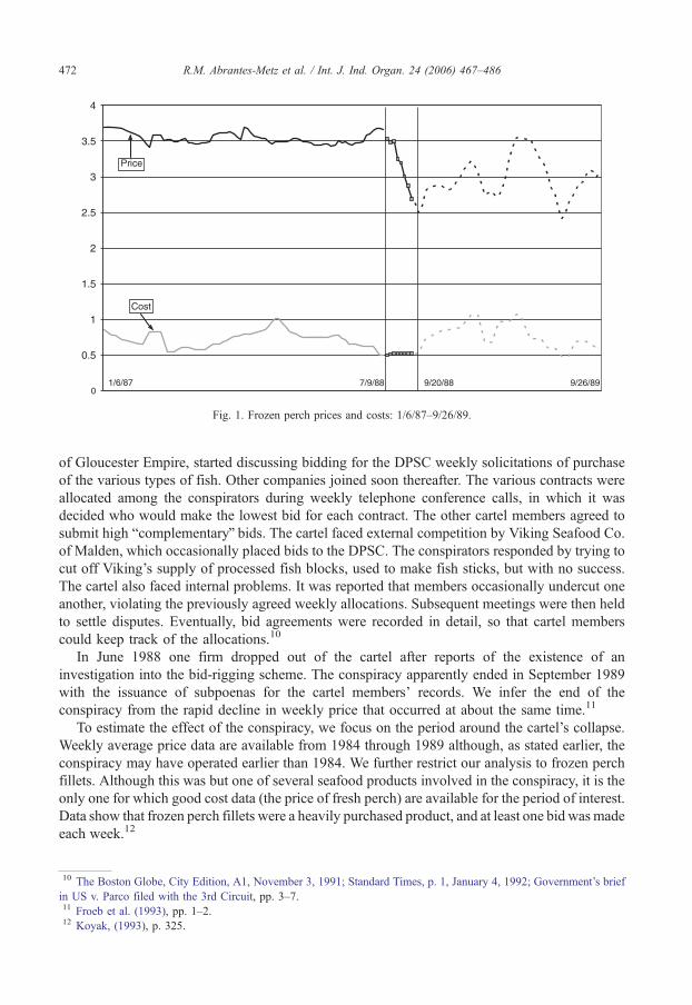
Fig. 1. Frozen perch prices and costs: 1/6/87–9/26/89.
R.M. Abrantes-Metz et al. / Int. J. Ind. Organ. 24 (2006) 467–486472
of Gloucester Empire, started discussing bidding for the DPSC weekly solicitations of purchase
of the various types of fish. Other companies joined soon thereafter. The various contracts were
allocated among the conspirators during weekly telephone conference calls, in which it was
decided who would make the lowest bid for each contract. The other cartel members agreed to
submit high bcomplementaryQ bids. The cartel faced external competition by Viking Seafood Co.
of Malden, which occasionally placed bids to the DPSC. The conspirators responded by trying to
cut off Viking’s supply of processed fish blocks, used to make fish sticks, but with no success.
The cartel also faced internal problems. It was reported that members occasionally undercut one
another, violating the previously agreed weekly allocations. Subsequent meetings were then held
to settle disputes. Eventually, bid agreements were recorded in detail, so that cartel members
could keep track of the allocations.10
In June 1988 one firm dropped out of the cartel after reports of the existence of an
investigation into the bid-rigging scheme. The conspiracy apparently ended in September 1989
with the issuance of subpoenas for the cartel members’ records. We infer the end of the
conspiracy from the rapid decline in weekly price that occurred at about the same time.11
To estimate the effect of the conspiracy, we focus on the period around the cartel’s collapse.
Weekly average price data are available from 1984 through 1989 although, as stated earlier, the
conspiracy may have operated earlier than 1984. We further restrict our analysis to frozen perch
fillets. Although this was but one of several seafood products involved in the conspiracy, it is the
only one for which good cost data (the price of fresh perch) are available for the period of interest.
Data show that frozen perch fillets were a heavily purchased product, and at least one bid wasmade
each week.12
10 The Boston Globe, City Edition, A1, November 3, 1991; Standard Times, p. 1, January 4, 1992; Government’s brief
in US v. Parco filed with the 3rd Circuit, pp. 3–7.11 Froeb et al. (1993), pp. 1–2.12 Koyak, (1993), p. 325.
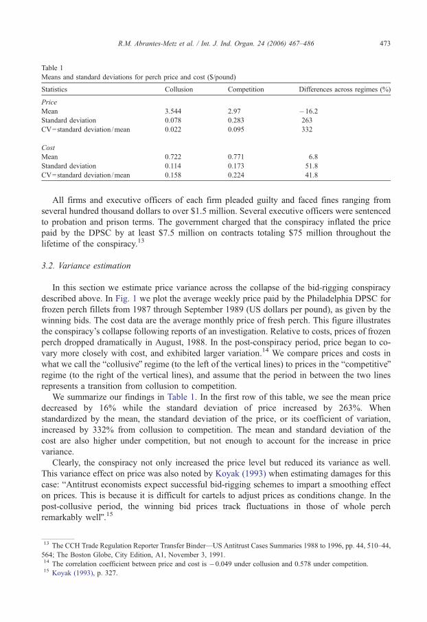
Table 1
Means and standard deviations for perch price and cost ($/pound)
Statistics Collusion Competition Differences across regimes (%)
Price
Mean 3.544 2.97 �16.2Standard deviation 0.078 0.283 263
CV=standard deviation /mean 0.022 0.095 332
Cost
Mean 0.722 0.771 6.8
Standard deviation 0.114 0.173 51.8
CV=standard deviation /mean 0.158 0.224 41.8
R.M. Abrantes-Metz et al. / Int. J. Ind. Organ. 24 (2006) 467–486 473
All firms and executive officers of each firm pleaded guilty and faced fines ranging from
several hundred thousand dollars to over $1.5 million. Several executive officers were sentenced
to probation and prison terms. The government charged that the conspiracy inflated the price
paid by the DPSC by at least $7.5 million on contracts totaling $75 million throughout the
lifetime of the conspiracy.13
3.2. Variance estimation
In this section we estimate price variance across the collapse of the bid-rigging conspiracy
described above. In Fig. 1 we plot the average weekly price paid by the Philadelphia DPSC for
frozen perch fillets from 1987 through September 1989 (US dollars per pound), as given by the
winning bids. The cost data are the average monthly price of fresh perch. This figure illustrates
the conspiracy’s collapse following reports of an investigation. Relative to costs, prices of frozen
perch dropped dramatically in August, 1988. In the post-conspiracy period, price began to co-
vary more closely with cost, and exhibited larger variation.14 We compare prices and costs in
what we call the bcollusiveQ regime (to the left of the vertical lines) to prices in the bcompetitiveQregime (to the right of the vertical lines), and assume that the period in between the two lines
represents a transition from collusion to competition.
We summarize our findings in Table 1. In the first row of this table, we see the mean price
decreased by 16% while the standard deviation of price increased by 263%. When
standardized by the mean, the standard deviation of the price, or its coefficient of variation,
increased by 332% from collusion to competition. The mean and standard deviation of the
cost are also higher under competition, but not enough to account for the increase in price
variance.
Clearly, the conspiracy not only increased the price level but reduced its variance as well.
This variance effect on price was also noted by Koyak (1993) when estimating damages for this
case: bAntitrust economists expect successful bid-rigging schemes to impart a smoothing effect
on prices. This is because it is difficult for cartels to adjust prices as conditions change. In the
post-collusive period, the winning bid prices track fluctuations in those of whole perch
remarkably wellQ.15
13 The CCH Trade Regulation Reporter Transfer Binder—US Antitrust Cases Summaries 1988 to 1996, pp. 44, 510–44,
564; The Boston Globe, City Edition, A1, November 3, 1991.14 The correlation coefficient between price and cost is �0.049 under collusion and 0.578 under competition.15 Koyak (1993), p. 327.
R.M. Abrantes-Metz et al. / Int. J. Ind. Organ. 24 (2006) 467–486474
4. The retail gasoline industry in Greater Louisville
4.1. Louisville retail market
In previous section we found that the collusive regime had lower standard deviation. We
hypothesize that other conspiracies would exhibit this feature, along with a higher price, and
design and apply a screen based on the coefficient of variation to retail gasoline stations in
Louisville.
The size of potential conspiracies is not known, but previous literature on retail gasoline has
found conspiracies in small localized markets. Slade (1992) found fairly localized markets, and
Hastings (2004) uses circular markets with radii of 0.5 and 1.5 miles. The US Department of
Justice has prosecuted conspiracies ranging in size from two gasoline stations to those involving
two to five jobbers and thirty to fifty stations.16 Due to the arguably localized nature of
competition in retail gasoline, we hypothesize that a conspiracy would include stations located
nearby to one another, and look for areas where retail gasoline prices exhibit low coefficients of
variation as an indicator of collusion.
Our retail gasoline price data comes from the Oil Price Information Service (OPIS). The data
are generated from a sample of retail outlets that accept fleet cards.17 OPIS records the actual
transaction price charged at the station on a given day. Hence, in principle, it is possible to create
a panel dataset consisting of specific stations’ daily gasoline price. While the gasoline price data
from OPIS is among the best available, a price is recorded for a specific station only if a
purchase is made at that station; that is, if no one with a fleet card purchases gasoline at a station
no price is recorded for that station on that day. In our data no single station has a complete time
series of prices, and some stations have very few price quotes (e.g., fewer than one per week).18
Consequently, stations that sell more gasoline are more likely to be sampled on any given day. In
addition, branded gasoline stations (which tend to charge higher prices) are more likely to accept
fleet cards, and thus be included in the sample.
The OPIS data consists of the station-specific price of regular grade gasoline, the brand of
gasoline, and the station location. In this sample from the Louisville region, we use a total of 279
gas stations with incomplete daily retail gasoline prices from February 4, 1996 through August
2, 2002.19 Our sample includes ten different brands of gasoline stations and another group of
unbranded stations. The brands are Amoco, Ashland, BP, Chevron, Citgo, Dairy Mart,
Marathon, Shell, Speedway and Super America. To fill in the missing observations in our dataset
we use multiple imputation, in particular, Markov chain Monte Carlo with Gibbs sampling
combined with data augmentation. This methodology is presented in the next subsection.
16 This information is based on conversations with William Dillon of the US Department of Justice. A jobber is an
intermediary who purchases gasoline at the distribution rack and pays a wholesale price called the rack price and then
resells the gasoline to branded station owners. Jobbers may also purchase gasoline at the rack for their own branded
stations.17 Fleet cards are often used by firms whose employees drive a lot for business purposes, e.g., salesman or insurance
claims adjusters. Fleet cards are often used to closely monitor what items employees charge to the firm, e.g., to ensure
that an employee only bills fuel and not food when visiting a filling station.18 Retail prices are reported for most weekdays with few exceptions. In 1998 and 1999 no retail prices are reported
during the week of Thanksgiving (because of very small sample sizes).19 According to New Image Marketing surveys there were 418 gasoline stations in the three Kentucky counties that
comprise Louisville in 1996 and 344 in 1999. Our sample of stations therefore represents between two-thirds and three-
quarters of the gasoline stations.
R.M. Abrantes-Metz et al. / Int. J. Ind. Organ. 24 (2006) 467–486 475
4.2. Data imputation, Markov chain Monte Carlo, Gibbs sampling and data augmentation
4.2.1. General overview
Data imputation bfills inQ the missing data with predicted or simulated values. Popular types
of imputation include mean substitution, simple hot deck and regression methods.
Mean substitution is appealing but corrupts the distribution of the series we are trying to
complete, which we denote Z. In simple hot deck, each missing value is replaced with a
randomly drawn observed value. This preserves the marginal distribution of Z, but is
inappropriate for our time series data. Regression methods replace missing values with either
the predicted values from a regression model, or with the predicted values plus random residuals.
They become awkward given the sequences of missing values we confront.
In any of these methods, when the missing data are replaced by a single set of imputed values,
the analysis that follows from the use of the complete dataset does not reflect missing data
uncertainty: the sample size N is overstated, the confidence intervals are too narrow, and the type
I error rates are too high. The problem becomes worse as the rate of missing observations and the
number of parameters increase. For all above reasons, in our context the proper data imputation
procedure to use is multiple imputation.
Multiple imputation is a simulation-based approach to the analysis of incomplete data. The
procedure is to (1) create imputations (i.e., replace each missing observation with m N1 simulated
values), (2) analyze each of them datasets in an identical fashion and (3) combine the results. Some
main advantages of multiple imputation in relation to single imputation (m =1) are that (i) the final
inferences incorporate missing data uncertainty, and (ii) it is highly efficient even for small m.
We create multiple imputations from the predictive distribution of the missing data. In
general, multiple imputations are drawn from a Bayesian predictive distribution
p zm; qjzoð Þ ¼Z
p zmjzo; hð Þp qjzoð Þdq; ð1Þ
with the data denoted by the vector zo, model parameters by the vector q, and the missing
observations by the vector zm. Section 4.2.2 provides details on the composition of these vectors.
Predictive distributions of the missing data are usually intractable, and require special
computation methods. One such method is Markov chain Monte Carlo, an iterative method for
drawing from intractable distributions. A Markov chain is created so that it converges to the
desired target. That can be accomplished through Gibbs sampling, the Metropolis–Hasting
algorithm, data augmentation, or a combination of these methods. In our multiple imputation of
the retail stations, the Markov chain Monte Carlo method used is Gibbs sampling combined with
data augmentation.
The principle behind Gibbs sampling is simple. We are interested in the numerical
approximation of E[ g(q)|zo] for a function of interest g(q)—for example, g(q) could be the
mean or standard deviation of prices for some subset of stations. Partition q into various blocks
as q =(hV(1),hV(2), . . .,hV(B)), where q( j) is a scalar or vector, j =1, 2, . . ., B. In many models
(including ours) it is not easy to directly draw from p(q|zo), but many times it is easy to
randomly draw from p(q(1)|zo , zm ,q(2), . . .,q(B )), p(q(2)|zo, zm ,q(1),q(3), . . .,q(B )), up to
p(q(B)|zo, zm,q(1),q(2), . . .,q(B� 1)) and finally from p(zm|zo,q). The last step is the data
augmentation. This algorithm yields a sequence q(1), q(2), . . ., q(s) drawn from the posterior
distribution p(q|zo) which can be averaged to produce estimates of Et g(q)|zob. It should be notedthat the state of the Gibbs sampler at draw s (i.e., q(s)) depends on its state at draw s�1 (i.e.,
q(s�1) and zm(s�1)), meaning that the sequence is a Markov chain.

R.M. Abrantes-Metz et al. / Int. J. Ind. Organ. 24 (2006) 467–486476
4.2.2. Imputation of missing price data
As previously explained, we use full Bayesian imputation to randomly assign values for the
missing observations. Once this is done, analysis can proceed as if there were no missing
observations. To summarize the strategy, let z denote all prices for a retail station, and
decompose this vector as zV=(zot, zmt), where o indicates observed values and m indicates
missing values. Let q denote the vector of unknown parameters in an econometric model for
retail prices, to be described shortly. The model specifies the distribution of retail prices, p(z|q),as well as a prior distribution for the unknown parameters, p(q). Then the distribution of the
unknowns, q and zm, conditional on the knowns, zo, is the predictive distribution
p zm; qjzoð Þ ¼ p zm; zo; qð Þ=p zoð Þ~p zm; zo; qð Þ ¼ p z; qð Þ ¼ p qð Þp zjqð Þ: ð2Þ
We use Markov chain Monte Carlo methods to sample from this distribution, discarding the
values of q and keeping the values of zm. The latter are the imputed missing values.
In particular, let yt denote an overall market price on day t; there are T days in the sample. In
practice, yt is computed as the average price taken over all stations reporting data for day t. If no
stations report data on day t, then yt is linearly interpolated for that day.
Let yit denote price at station i on day t, and let zit =yit�yt. There are n stations in the sample.
Interpolation is based on the stationary first-order autoregressive model
zit � li ¼ qi zit�1 � lið Þ þ eit:
The shocks eit are normal and independently distributed across stations and days, and identically
distributed across days for each station: eiidit fN 0; r2i
� �. The stationary initial condition is
zit � lfN 0; r2i = 1� q2ð Þ
� �.
The model permits a station to have prices that tend to be higher (liN0) or lower (li b0) than
average. On any given day there is a tendency for price at station i to return to its equilibrium
value yt+l. The speed of adjustment is governed by qi. For the stations in our sample qi
averages about 0.9; some stations are lower, others higher. On any given day there is also a
shock eit that perturbs prices. The standard deviation of this shock varies across stations, with a
typical station having a standard deviation of about 0.015.
If we were able to fully observe all T prices for station i, then
p zi1; . . . ; ziT jli; qi;r2i
� �¼ 2kð Þ�T=2 r2
i
� ��T=21� q2
i
� ��1=2: exp
*�(
1� q2i
� �zi1 � lið Þ2
þXTt¼2
zit � li � qi zit�1 � lið Þ½ �2),
2r2i
+: ð3Þ
This constitutes the density p(z|q) in the summary of our strategy given in Eq. (2). The unknown
parameters constitute qV=(l1,r12,q1, . . .,ln,rn
2,qn) (note that our analysis takes place one
station at a time, because conditional on yt(t=1, . . .,T) and q, station prices are independent of
one another). The prior distributions of the three parameters are independent and uninformative:
there is a flat, improper prior distribution for li on the real line; a flat, improper prior distribution
for ri2 on the positive half-line; and a flat, proper prior distribution for qi on the interval (�1, 1).
Thus the density from which we wish to sample is Eq. (3), but with the restriction that
qia (�1,1).The Markov chain Monte Carlo method is Gibbs sampling. Each of the three parameters and
each of the missing prices are drawn, in succession, from the conditional distribution implicit in
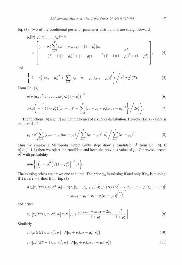
R.M. Abrantes-Metz et al. / Int. J. Ind. Organ. 24 (2006) 467–486 477
Eq. (3). Two of the conditional posterior parameter distributions are straightforward:
lijtr2i ; qi; zi1; . . . ; ziT bfN
�1� qið Þ
XTt¼2
zit � qizit�1ð Þ þ 1� q2i
� �zi1
T � 1ð Þ 1� qið Þ2 þ 1� q2ið Þ
;r2i
T � 1ð Þ 1� qið Þ2 þ 1� q2ið Þ
266664
377775; ð4Þ
and
1� q21
� �zi1 � lið Þ2 þ
XTt¼2
zit � lit � qi zit�1 � lið Þ½ �2( ),
r2ifv2 Tð Þ: ð5Þ
From Eq. (3),
p qijli; r2i ; zi1; . . . ; ziT
� �~ 1� q2
i
� �1=2 ð6Þ
:exp
*� 1� q2
i
� �zi1 � lið Þ2 þ
XTt¼2
zit � li � qi zit�1 � lið Þ½ �2( ),
2r2i
+: ð7Þ
The functions (6) and (7) are not the kernel of a known distribution. However Eq. (7) alone is
the kernel of
qifN t
XTt¼2
zit�1 � lið Þ zit � lið Þ�XT
t¼1zit � lið Þ2; r2
i
�XTt¼1
zit � lið Þ2: ð8Þ
Thus we employ a Metropolis within Gibbs step: draw a candidate qi* from Eq. (8). If
qi*g (�1,1) then we reject the candidate and keep the previous value of qi. Otherwise, accept
qi* with probability
min 1� q42
i
� �= 1� q2
i
� �h i1=2; 1
� �:
The missing prices are drawn one at a time. The price yis is missing if and only if zis is missing.
If 2V sVT�1 then from Eq. (3)
ptzisjzit t psð Þ; li; r2i ; qib ¼ p zisjzis�1; zisþ1; li; r
2i ; qi
� �~exp
D� zis � li � qi zis�1 � lið Þ½ �2n
þ zisþ1 � li � qi � qi zis � lið Þ½ �2oE
and hence
zisj zit t psð Þ; li; r2i ; qi
fN li þ
qi zis�1 þ zisþ1 � 2lið Þ1þ q2
i
;r2i
1þ q2i
� �: ð9Þ
Similarly
zi1jtzit tz2ð Þ; li; r2i ; qibfN tli þ qi zi2 � lið Þ; r2
i b; ð10Þ
ziT jtzit tVT � 1ð Þ; li; r2i ; qibfN tli þ qi ziT�1 � lið Þ; r2
i b; ð11Þ
R.M. Abrantes-Metz et al. / Int. J. Ind. Organ. 24 (2006) 467–486478
of course, yis =ys + zis. To sample the unknown parameters and missing data from Eq. (2), the
Markov chain Monte Carlo algorithm samples, in turn,from Eqs. (4), (5), (8) followed by the
acceptance–rejection step, Eqs. (10), (9) for s =2, . . ., T�2 and (11). The algorithm is initialized
with li =0, qi=0.9, ri2=0.0152, and zis =0 zis for all missing data. Convergence is essentially
instantaneous, even for stations for which a substantial fraction of observations are missing. Our
interpolation is based on ten iterations of the MCMC algorithm, which requires only a few
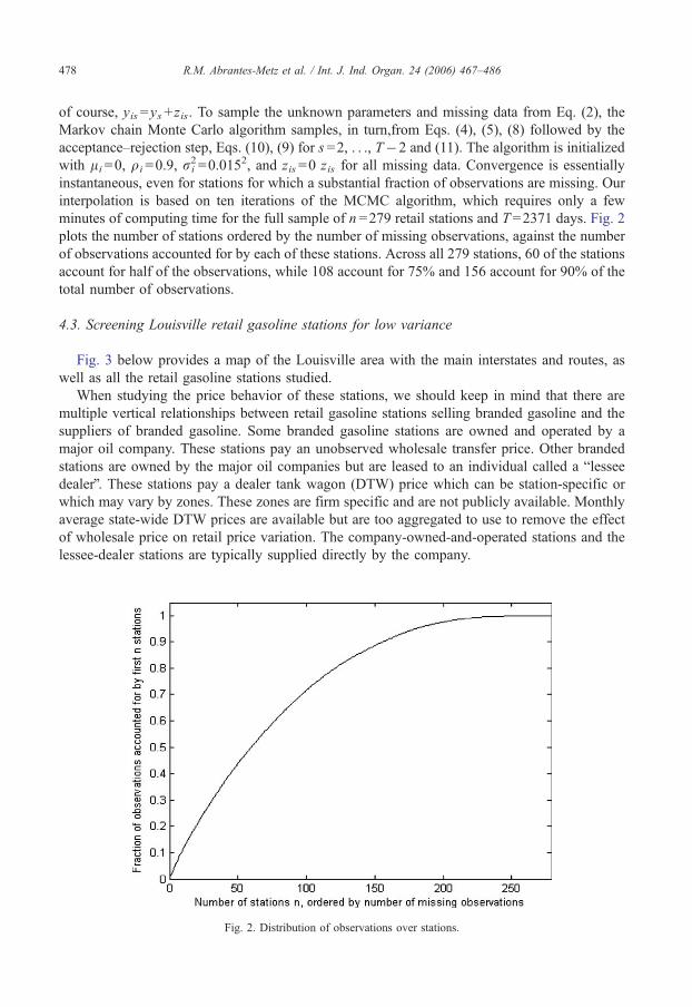
minutes of computing time for the full sample of n =279 retail stations and T=2371 days. Fig. 2
plots the number of stations ordered by the number of missing observations, against the number
of observations accounted for by each of these stations. Across all 279 stations, 60 of the stations
account for half of the observations, while 108 account for 75% and 156 account for 90% of the
total number of observations.
4.3. Screening Louisville retail gasoline stations for low variance
Fig. 3 below provides a map of the Louisville area with the main interstates and routes, as
well as all the retail gasoline stations studied.
When studying the price behavior of these stations, we should keep in mind that there are
multiple vertical relationships between retail gasoline stations selling branded gasoline and the
suppliers of branded gasoline. Some branded gasoline stations are owned and operated by a
major oil company. These stations pay an unobserved wholesale transfer price. Other branded
stations are owned by the major oil companies but are leased to an individual called a blesseedealerQ. These stations pay a dealer tank wagon (DTW) price which can be station-specific or
which may vary by zones. These zones are firm specific and are not publicly available. Monthly
average state-wide DTW prices are available but are too aggregated to use to remove the effect
of wholesale price on retail price variation. The company-owned-and-operated stations and the
lessee-dealer stations are typically supplied directly by the company.
Fig. 2. Distribution of observations over stations.
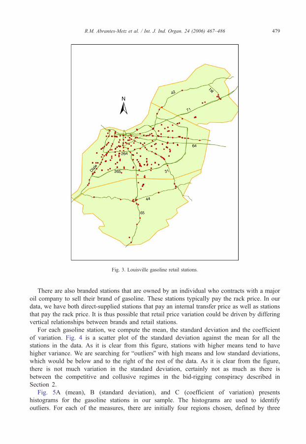
Fig. 3. Louisville gasoline retail stations.
R.M. Abrantes-Metz et al. / Int. J. Ind. Organ. 24 (2006) 467–486 479
There are also branded stations that are owned by an individual who contracts with a major
oil company to sell their brand of gasoline. These stations typically pay the rack price. In our
data, we have both direct-supplied stations that pay an internal transfer price as well as stations
that pay the rack price. It is thus possible that retail price variation could be driven by differing
vertical relationships between brands and retail stations.
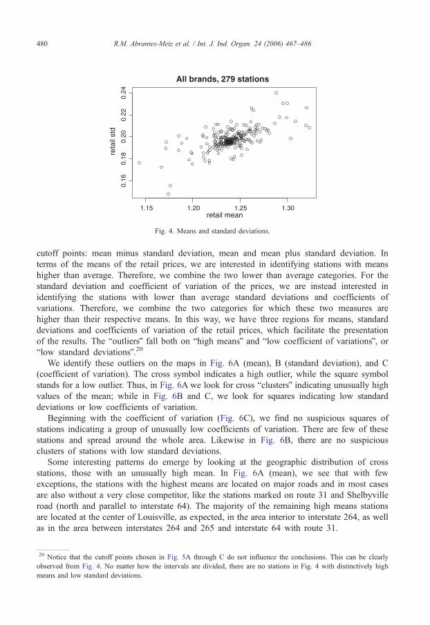
For each gasoline station, we compute the mean, the standard deviation and the coefficient
of variation. Fig. 4 is a scatter plot of the standard deviation against the mean for all the
stations in the data. As it is clear from this figure, stations with higher means tend to have
higher variance. We are searching for boutliersQ with high means and low standard deviations,
which would be below and to the right of the rest of the data. As it is clear from the figure,
there is not much variation in the standard deviation, certainly not as much as there is
between the competitive and collusive regimes in the bid-rigging conspiracy described in
Section 2.
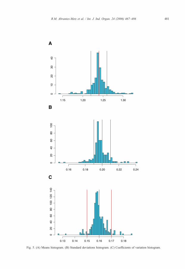
Fig. 5A (mean), B (standard deviation), and C (coefficient of variation) presents
histograms for the gasoline stations in our sample. The histograms are used to identify
outliers. For each of the measures, there are initially four regions chosen, defined by three
1.15 1.20 1.25 1.30
0.16
0.18
0.20
0.22
0.24
retail mean
reta
il st
d
All brands, 279 stations
Fig. 4. Means and standard deviations.
R.M. Abrantes-Metz et al. / Int. J. Ind. Organ. 24 (2006) 467–486480
cutoff points: mean minus standard deviation, mean and mean plus standard deviation. In
terms of the means of the retail prices, we are interested in identifying stations with means
higher than average. Therefore, we combine the two lower than average categories. For the
standard deviation and coefficient of variation of the prices, we are instead interested in
identifying the stations with lower than average standard deviations and coefficients of
variations. Therefore, we combine the two categories for which these two measures are
higher than their respective means. In this way, we have three regions for means, standard
deviations and coefficients of variation of the retail prices, which facilitate the presentation
of the results. The boutliersQ fall both on bhigh meansQ and blow coefficient of variationsQ, orblow standard deviationsQ.20
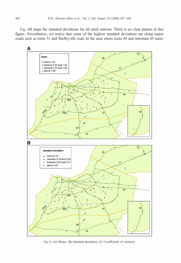
We identify these outliers on the maps in Fig. 6A (mean), B (standard deviation), and C
(coefficient of variation). The cross symbol indicates a high outlier, while the square symbol
stands for a low outlier. Thus, in Fig. 6A we look for cross bclustersQ indicating unusually high
values of the mean; while in Fig. 6B and C, we look for squares indicating low standard
deviations or low coefficients of variation.
Beginning with the coefficient of variation (Fig. 6C), we find no suspicious squares of
stations indicating a group of unusually low coefficients of variation. There are few of these
stations and spread around the whole area. Likewise in Fig. 6B, there are no suspicious
clusters of stations with low standard deviations.
Some interesting patterns do emerge by looking at the geographic distribution of cross
stations, those with an unusually high mean. In Fig. 6A (mean), we see that with few
exceptions, the stations with the highest means are located on major roads and in most cases
are also without a very close competitor, like the stations marked on route 31 and Shelbyville
road (north and parallel to interstate 64). The majority of the remaining high means stations
are located at the center of Louisville, as expected, in the area interior to interstate 264, as well
as in the area between interstates 264 and 265 and interstate 64 with route 31.
20 Notice that the cutoff points chosen in Fig. 5A through C do not influence the conclusions. This can be clearly
observed from Fig. 4. No matter how the intervals are divided, there are no stations in Fig. 4 with distinctively high
means and low standard deviations.
A
B
C
1.15 1.20 1.25 1.30
010
2030
40
0.16 0.18 0.20 0.22 0.24
020
4060
8010
0
0.17 0.18
020
4060
8010
012
014
0
0.160.150.140.13
Fig. 5. (A) Means histogram. (B) Standard deviations histogram. (C) Coefficients of variation histogram.
R.M. Abrantes-Metz et al. / Int. J. Ind. Organ. 24 (2006) 467–486 481
R.M. Abrantes-Metz et al. / Int. J. Ind. Organ. 24 (2006) 467–486482
Fig. 6B maps the standard deviations for all retail stations. There is no clear pattern in this
figure. Nevertheless, we notice that some of the highest standard deviations are along major
roads such as route 31 and Shelbyville road. In the area where route 44 and interstate 65 meet,
Fig. 6. (A) Means. (B) Standard deviations. (C) Coefficients of variation.

std/mean ratio
below 0.15between 0.15 and 0.16between 0.16 and 0.17above 0.17
Dixie
265
264
31
65
44
64
71
42
1st
65
C
Fig. 6 (continued).
brands (total 249)
AMOCO (17)ASHLAAND (8)BP (68)CHEVRON (45)CITGO (21)DAIRY MART (14)MARATHON (26)SHELL (26)SPEEDYWAY (8)SUPER AMERICA (36)UNBRANDED (10)
264
265Dixie
65
44
31 65
64
71
1st
42
Fig. 7. Brands.
R.M. Abrantes-Metz et al. / Int. J. Ind. Organ. 24 (2006) 467–486 483

R.M. Abrantes-Metz et al. / Int. J. Ind. Organ. 24 (2006) 467–486484
most stations have price variation lower than average, as well as for many of the stations
located on Dixie Road. As previously discussed, this could be due to the fact that some
stations are company owned and operated and pricing is centrally controlled (less volatile
retail price), while for others pricing is decided by the local owner (more volatile retail price).
The stations with the lowest standard deviations identified with a square are very few,
scattered across the whole geographical area and either without very close competitor, or with
a competitor with a higher standard deviation. Hence, we find no groups of stations with low
price variation.
When combining these findings with the brands of gasoline in the sample (Fig. 7), we find no
clear association between high means and low coefficients of variation and the several brands,
though most of the stations referred to on Dixie Road and Shelbyville road sell BP or Super
America gasoline.
Overall, only a few of the stations along Dixie Road have slightly higher means, slightly
lower standard deviations and lower coefficients of variation than most others in the area,
but these differences are not significant, especially when measured against the large changes
in variance estimated in the previous section. While the coefficient of variation increased
almost four and a half times from collusion to competition in the perch example, in the gasoline
retail market the highest value for the coefficient of variation is only about one and a half
times higher than the lowest value. We do not think the differences across retail stations are big
enough to suggest collusive behavior in Louisville in 1996–2002.
5. Conclusion
We know far too little about how real cartels actually operate. Retrospective studies of
cartel prosecutions, particularly when they result in the collapse of a cartel, allow researchers
to compare a collusive regime to a competitive one to isolate the critical features of
the conspiracy. In the collapse of our bid-rigging conspiracy, we found a relatively small
difference in price, but a huge difference in variance. It would be useful to know whether
other conspiracies exhibited low variance, and if they did, which factors led to the low
variance. This is clearly a difficult task, as the volatility of prices depends on so many
different factors beyond price setting, and in a different way depending on the industries
considered, which makes the comparison across industries difficult to establish.
Empirical evidence like this can be used to test some of the hypotheses generated by the
enormous amount of theoretical work in this area and can be used to guide policy. For
example, there is very little evidence on how mergers affect the likelihood of collusion in a
given industry. More retrospective studies might generate empirical regularities that could be
used to tell enforcers both where to look for conspiracies, and which factors would hasten
the collapse of a conspiracy or prevent a cartel from otherwise forming. This kind of
information would also help merger enforcers determine when a merger might result in a
cartel, or prevent a cartel from otherwise collapsing. Economists have given enforcers very
little guidance in understanding how a merger results in bcoordinated effectsQ.21
The failure of our screen to identify bsuspiciousQ areas could not only mean that
the gasoline stations in Louisville are competing, but it could also indicate a failure of the
screen to uncover pockets of existing collusion. Ideally, we would use a cartel collapse in
the same industry to design an empirical screen for collusion. As more and better
21 U.S. Department of Justice and Federal Trade Commission (1997).
R.M. Abrantes-Metz et al. / Int. J. Ind. Organ. 24 (2006) 467–486 485
retrospective studies are done, we expect that more features of conspiracies will be
uncovered that will help us design screens. Given the history of data screens to identify
cartels, we remain uncertain whether screening for conspiracies is a good use of scarce
enforcement resources.
Acknowledgements
We would like to thank participants at the International Industrial Organization Conference,
at the seminar series of Portugal’s Autoridade da Concorrencia, Sumanth Addanki, William
Dillon, Joseph Harrington, Albert Metz, Timothy Muris, Frederick Warren-Boulton and our
colleagues at the FTC and NERA for helpful comments and suggestions, in particular,
Chantale LaCasse, Gregory Leonard, Richard Rapp and Ramsey Shehadeh. We also thank
Jonathan Chatzkel, David Yans and Ning Yan for excellent assistance, as well as comments
from two anonymous reviewers of the FTC working paper series and two anonymous
reviewers for this journal. The views expressed are those of the authors and do not necessarily
reflect the views of the FTC Commission or any individual Commissioner, nor the views of
NERA or its clients.
References
Anthony Parco, at 83; Founded Fertilizer Firm, 2004. The Boston Globe—third. P B10, May 23.
Athey, Susan, Bagwell, Kyle, Sanchirico, Chris William, 2004. Collusion and price rigidity. Review of Economic Studies
71 (2), 317–349.
Bajari, Patrick, Ye, Lixin, 2003. Deciding between competition and collusion. Review of Economics and Statistics 85 (4),
971–989.
Bolotova, Yuliya, Connor, John M., Miller, Douglas J., 2005. The Impact of Collusion on Price Behavior: Empirical
Results from Two Recent Cases. Purdue University Department of Agricultural Economics.
Connor, John, M., 2005. Collusion and Price Dispersion. Applied Economic Letters 12 (6/15), 225–228.
Feinstein, Jonathan, S., Block, Michael, Nold, Frederick, 1985. Asymmetric information and collusive behavior in
auction markets. American Economic Review 75 (3), 441–460.
Froeb, Luke, Shor, Mikhael, 2005. Auction models. In: Harkrider, John D. (Ed.), Econometrics: Legal, Practical, and
Technical Issues. American Bar Association Section of Antitrust Law, pp. 225–246.
Froeb, Luke M., Koyak, Robert A., Werden, Gregory J., 1993. What is the effect of bid-rigging on prices? Economic
Letters 42, 419.
Genesove, David, Mullin, Wallace, 2001. Rules, communication and collusion: narrative evidence from the sugar
institute case. American Economic Review 91 (3), 379–398.
Harington, Joseph E., 2004. Detecting cartels. Working Paper, Johns Hopkins University Hastings.
Harrington, Joseph E., Chen, Joe, 2004. Cartel pricing dynamics with cost variability and endogenous buyer detection.
Working Paper, Johns Hopkins University.
Hastings, Justine, 2004. Vertical relationships and competition in retail gasoline markets: empirical evidence from
contract changes in southern California. American Economic Review 94 (1), 317–328.
LaCasse, Chantale, 1995. Bid rigging and the threat of government prosecution. RAND Journal of Economics 26 (3),
398–417.
Lee, Tai Sik, 1990. Detection of Collusion in Highway Construction Contract Bidding, Dissertation, University of
Wisconsin—Madison.
Koyak, Robert, 1993. 1993 Proceedings of the Business and Economic Statistics Section. American Statistical
Association, pp. 325–330.
Porter, Robert H., Zona, J. Douglas, 1993. Detection of bid rigging in procurement auctions. Journal of Political
Economy 101 (3), 518–538.
Slade, Margaret E., 1992. Vancouver’s gasoline-price wars: an empirical exercise in uncovering supergame strategies.
Review of Economic Studies 59 (2), 257–276 (April).
Taylor, Christopher, Fischer, Jeffrey, 2003. A review of West Coast pricing and the impact of regulations. International
Journal of the Economics of Business 10 (2), 225–243.

R.M. Abrantes-Metz et al. / Int. J. Ind. Organ. 24 (2006) 467–486486
Taylor, Christopher and Daniel Hosken, 2004. The economic effects of the Marathon–Ashland joint venture: the
importance of industry supply shocks and vertical market structure. Federal Trade Commission Bureau of Economics,
Working paper, 270.
The Unraveling of a New England Fish Scam, 1991. The Boston Globe—City Edition, p. A.1. November 3.
Tichon fined $675,000 in bid rigging, 1992, January 4. Standard Times, p.1.
United States v. Parco, 1992. No. 92-1008 (3rd Cir.).
US Department of Justice and Federal Trade Commission, April 2 1992. Horizontal merger guidelines. Revised April 8
1997.