a variational approach to cardiac motion estimation...
TRANSCRIPT

QUARTERLY OF APPLIED MATHEMATICS
VOLUME , NUMBER 0
XXXX XXXX, PAGES 000–000
S 0033-569X(XX)0000-0
A VARIATIONAL APPROACH TO CARDIAC MOTIONESTIMATION BASED ON COVARIANT DERIVATIVES AND
MULTI-SCALE HELMHOLTZ DECOMPOSITION.
By
REMCO DUITS (Department of Mathematics/Computer Science and Department of BiomedicalEngineering, Eindhoven University of Technology, Den Dolech 2, P.O. Box 513, 5600MB Eindhoven,
The Netherlands.),
BART JANSSEN (Department of Mathematics/Computer Science, Eindhoven University ofTechnology, Den Dolech 2, P.O. Box 513, 5600MB Eindhoven, The Netherlands.),
ALESSANDRO BECCIU (Department of Biomedical Engineering, Eindhoven University ofTechnology, Den Dolech 2, P.O. Box 513, 5600MB Eindhoven, The Netherlands.),
and
HANS VAN ASSEN (Department of Biomedical Engineering, Eindhoven University of Technology,Den Dolech 2, P.O. Box 513, 5600MB Eindhoven, The Netherlands.)
Abstract. The investigation and quantification of cardiac motion is important forassessment of cardiac abnormalities and treatment effectiveness. Therefore we considera new method to track cardiac motion from magnetic resonance (MR) tagged images.Tracking is achieved by following the spatial maxima in scale-space of the MR images overtime. Reconstruction of the velocity field is then carried out by minimizing an energyfunctional which is a Sobolev-norm expressed in covariant derivatives. These covariantderivatives are used to express prior knowledge about the velocity field in the variationalframework employed. Furthermore, we propose a multi-scale Helmholtz decompositionalgorithm that combines diffusion and Helmholtz decomposition in one non-singular an-alytic kernel operator in order to decompose the optic flow vector field in a divergencefree, and rotation free part. Finally, we combine both the multi-scale Helmholtz de-composition and our vector field reconstruction (based on covariant derivatives) in a
2000 Mathematics Subject Classification. Primary 55R10,49M25,47A05 ; Secondary 47A10, 49M27.Key words and phrases. Covariant Derivatives, Fiber bundles, Helmholtz decomposition, Inverse prob-lems, Optical flow methods in image analysis, Scale Space.Current address: Department of Mathematics/Computer Science and Department of Biomedical En-gineering, Eindhoven University of Technology, Den Dolech 2, P.O. Box 513, 5600MB Eindhoven, TheNetherlands.E-mail address: [email protected]
E-mail address: [email protected]
E-mail address: [email protected]
E-mail address: [email protected]
c©XXXX Brown University
1

2 REMCO DUITS, BART JANSSEN, ALESSANDRO BECCIU, AND HANS VAN ASSEN
single algorithm and show the practical benefit of this approach by an experiment onreal cardiac images.
1. Introduction. In cardiology literature [52] it has been noted that deformation ofthe cardiac wall provides a quantitative indication of the health of the cardiac muscle.Cardiac motion extraction is therefore an important area of research. Monitoring andquantification of irregular cardiac wall deformation may help in early diagnosis of car-diac abnormalities such as ischemia and provides information about the effectiveness oftreatment, cf. [10, 46]. In order to characterize contraction and dilation of the cardiacmuscle, non-invasive acquisition techniques such as magnetic resonance (MR) taggingcan be applied. MR tagging allows to superimpose artificial brightness patterns on theimage, which deform according to the cardiac muscle’s motion and aid to retrieve motionwithin the heart walls, cf. Fig. 1. The problem of extracting motion in image sequences
Fig. 1. Left: Short axis view of a patient’s left ventricle. Middle:Sine-phase images. Right: Sum of sine-phase images for a fixed timet. This sum of sine phase images serves as input to our algorithmsand will be denoted by f(x, t) where x = (x, y) ∈ R2, t > 0.
is of primary interest for the computer vision and image analysis community. Optic flowmeasures apparent motion of moving patterns in image sequences, providing informationabout spatial displacements of objects in consecutive frames. At the beginning of theeighties Horn and Schunck introduced a mathematical formulation of optic flow assumingthat intensities associated to image objects do not change along the sequence, [29]. Thisformulation has been referred to as the Optic Flow Constraint Equation (OFCE):
fxu + fyv + ft = 0 (1.1)
where (x, y, t) → f(x, y, t) : R2 × R+ → R is an image sequence, fx, fy, ft are thespatial and temporal derivatives; v(·, t) is a vector field on R2 given by v(x, y, t) =(u(x, y, t), v(x, y, t))T , where u and v are unknown and x, y and t are the spatial andtemporal coordinates respectively. Since scalar-valued functions u and v are unknown,Eq. (1.1) does not have a unique solution, providing the so-called ”aperture problem”.Horn and Schunck dealt with the aperture problem by proposing a variational frameworkrelated to Eq. (1.1), cf. [29]. For further extensions/improvements see [6, 19, 55, 59, 63].
The constant brightness assumption (1.1) does not apply to a wide variety of medicalimaging problems, such as cardiac motion estimation from MR-tagged images. Fur-thermore, most of these methods do not take into account physical properties of thevelocity field generated by rotation and dilation of the cardiac tissue. Local rotationand contraction of the cardiac muscle can be estimated by Helmholtz decomposition,

MOTION ESTIMATION BY COVARIANT DERIVATIVES AND HELMHOLTZ DECOMPOSITION 3
cf. [1, 60, 40, 7, 8], of the vector field. Exploring this decomposition can play a fun-damental role in the clinical diagnosis procedure, since it may reveal abnormalities intissue deformation. Therefore, for applications such as cardiac motion extraction, bloodflow calculation and fluid motion analysis, this may lead to more accurate velocity fieldestimation in comparison to general approaches, cf. [7, 40, 26].
In this work we extract 2-dimensional cardiac wall motion by employing an optic flowmethod based on features such as spatial extrema in a linear scale space representationof the image sequence. The flow field is reconstructed via a variational method; inthe regularization term we include our multi-scale Helmholtz decomposition and we usecovariant derivatives biased by a so-called gauge field. Advantages of this approach aresignificant:
(i) We do not suffer from the aperture problem.(ii) Critical points such as spatial maxima are robust with respect to monotonic
transformations in the codomain, such as fading, in the image. Therefore, thealgorithm can be robustly applied on image sequences (like tagged MR images)where the intensity constancy is not preserved.
(iii) The proposed technique allows a separate analysis of the divergence and rota-tion free part of the cardiac motion by means of a robust multi-scale Helmholtzdecomposition.
(iv) The algorithm has the advantages provided by a multi-scale approach:– A scale selection scheme for the feature points (extrema) is included, where
we take into account both topological transitions and spatial dislocation ofextremal paths in scale space. For details, see [12, ch:4.1].
– We avoid typical grid artefacts by analytical pre-computation of the concate-nation of linear diffusion and Helmholtz decomposition, cf. Cuzol et al. [8].Besides the gradient of the potential in [8] we also express the subsequentderivative operators in Gaussian derivatives. This yields a single analyticvector-valued kernel that can be pre-computed (avoiding vortex-particle ap-proximations). We do not use discrete multi-scale Helmholtz decomposi-tions, cf. [56], which act by means of nonlinear diffusions on the potentials,since we need to keep track of scale by means of linear diffusion on the field.
(v) We obtain a better flow field reconstruction, compared to similar techniquescf. [5, 34], by replacing standard derivatives by covariant derivatives which allowsus to incorporate prior knowledge (based on features) in the regularization term.An alternative approach to include prior knowledge in the regularization termcan be found in the work by Nir et al. [48].
(vi) Both the computation of the gauge field and the reconstruction framework arestable linear operators (due to the coercivity of the covariant Laplacian).
Throughout this article we will consider cardiac motion. Our general technique can alsobe applied to cardiac strain and deformation, which is also relevant in cardiac imaging,cf. [58, 20], However, strain can also be directly computed from frequency fields using(enhanced) Gabor transforms, cf. [13].
Outline of algorithm and article. An overview of the proposed algorithm is providedin Figure 2 and every step is described as follows. Section 3 describes the methodology

4 REMCO DUITS, BART JANSSEN, ALESSANDRO BECCIU, AND HANS VAN ASSEN
used to calculate velocity features including a scale selection. Section 4 is dedicated tothe multi-scale Helmholtz decomposition of vector fields, where we analytically computethe effective kernel operator that arises from the concatenation of the (commuting) lineardiffusion operator and the Helmholtz-decomposition operator.
In Sections 5, 6 we introduce the concept of covariant derivatives. Subsequently, inSection 7 we investigate the covariant Laplacian and in Section 8 we derive its associatedGreen’s function of the covariant Laplacian. Furthermore, we deduce a lower bound onthe spectrum of the covariant Laplacian.
In Section 9 we consider motion field reconstruction by minimization of an energyfunctional where the data term is obtained by our approach explained in Section 3 andwhere the smoothness term is expressed in the covariant derivatives of Section 6. Themotion field reconstruction is obtained by solving continuous Euler-Lagrange equations.In Section 10 we also derive the corresponding discrete equations arising by expansionin a B-spline basis. Stability is manifest, both in the continuous and discrete EulerLagrange systems as we show in Section 11 where we rely on our results in Section 8.
Then in Section 12 we put everything together and include the multi-scale Helmholtzdecomposition in the motion field reconstruction. Here we distinguish between two op-tions, a pragmatic one which consists of two separate reconstruction algorithms for thedivergence and rotation free parts and a more elaborate approach where we merge ev-erything into a single energy minimization yielding a related, but more difficult, Euler-Lagrange system as explained in Section 14.
Finally in Section 15 we apply our algorithm to real data obtained from a patientand a healthy volunteer. For further details on experiments on phantoms with knownground truth and extensive assessment of the algorithm performance (qualitatively andquantitatively) we refer to our technical report [12]. These experiments clearly showthe advantage of including both covariant derivatives and Helmholtz decomposition. Inthis paper we rather put emphasis on the mathematical underpinning, stability andfundamental properties of our approach.
2. Input: Tagged MR images. Tagging is a noninvasive technique based on locallyperturbing the magnetization of the cardiac tissue via radio frequency pulses. MR tagsare artificial patterns, that appear as dark stripes on the MR images with the aim toimprove the visualization of the deforming tissue [62]. An example of a tagged heartimage is displayed in figure 1, column 1. In order to increase the number of tags inthe image, Axel and Dougherty [2] spatially modulated the degree of magnetization inthe cardiac tissue, whereas Osman et al. [49] proposed the so-called harmonic phase(HARP) method, which converts MR images in phase images. In our experiments weapply a similar technique where we extract sine phase images by means of Gabor filters[22, 59] (figure 1, column 2). Such images allow to extract feature points such as maximaminima and saddles with high accuracy. The calculated since phase images have beencombined in order to create a chessboard-like pattern. Throughout this article we willapply our methods to phase images as depicted in Figure 1, column 3.

MOTION ESTIMATION BY COVARIANT DERIVATIVES AND HELMHOLTZ DECOMPOSITION 5
Fig. 2. Overview of the algorithm. Input tagged images and firstpreprocessing steps are discussed in Section 2. The feature track-ing procedure is described in Section 3. Sections 5 and 6 explainthe concept of covariant derivatives and in Section 4 we presentour multi-scale Helmholtz decomposition algorithm. The box onthe right shows how these two techniques are applied in the densemotion field reconstruction that we present in Sections 9, 10 and 12.
3. Computation of velocity features via critical paths in scale space. Theso-called Gaussian scale space representation I : R2 × R+ → R of a 2D static imagex 7→ f(x) ∈ L2(R2) is defined by the spatial convolution of the image with a Gaussiankernel
I(x, s) = (f ∗ φs)(x) , with φs(x) =1
4πsexp(−‖x‖
2
4s) , s > 0, (3.1)
where x = (x, y) ∈ R2 and where s > 0 represents the scale of observation [30, 61, 42,43, 39, 54, 16]. Note that (3.1) is the solution of a diffusion system on the upper halfspace s > 0, so ∂
∂sI = ∆I and lims↓0
I(·, s) = f , lims→∞
I(·, s) = 0 where both limits are taken
in L2-sense. This procedure naturally extends to a multiple scale representation of adynamic image (x, y, t) 7→ f(x, y, t):
I(x, y, s, t) := (φs ∗ f(·, ·, t))(x, y), t, s > 0,x = (x, y) ∈ R2.
For each fixed time t > 0 we compute the critical paths in R2 × R+ where the spatialgradient vanishes ∇I(x, s, t) = 0. We used a sub-pixel accurate method to determine thecritical paths based on topological numbers, for details see [53, 12]. By means of Morsesingularity theory [9, 18] one can deduce that these critical paths generically vanish1 atso-called top-points as scale increases. These top-points are given by
∇I(x, s, t) = 0 and det HI(x, s, t) = Ixx(x, s, t)Iyy(x, s, t)− (Ixy(x, s, t))2 = 0 (3.2)
In the visualization of critical paths in scale space, scale s is parameterized logarithmically
s/smin = e2τ ⇔ τ =12
log(s/smin) ,
1During diffusion creation of critical paths occurs as well, cf. [9, 18], but these topological transitionsare less frequent and are usually followed by an annihilation at a slightly higher scale.
6 REMCO DUITS, BART JANSSEN, ALESSANDRO BECCIU, AND HANS VAN ASSEN
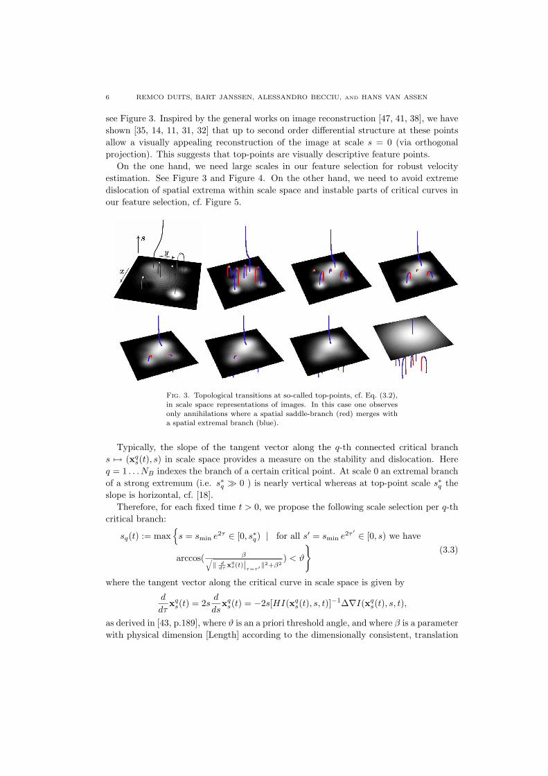
see Figure 3. Inspired by the general works on image reconstruction [47, 41, 38], we haveshown [35, 14, 11, 31, 32] that up to second order differential structure at these pointsallow a visually appealing reconstruction of the image at scale s = 0 (via orthogonalprojection). This suggests that top-points are visually descriptive feature points.
On the one hand, we need large scales in our feature selection for robust velocityestimation. See Figure 3 and Figure 4. On the other hand, we need to avoid extremedislocation of spatial extrema within scale space and instable parts of critical curves inour feature selection, cf. Figure 5.
Fig. 3. Topological transitions at so-called top-points, cf. Eq. (3.2),in scale space representations of images. In this case one observesonly annihilations where a spatial saddle-branch (red) merges witha spatial extremal branch (blue).
Typically, the slope of the tangent vector along the q-th connected critical branchs 7→ (xq
s(t), s) in scale space provides a measure on the stability and dislocation. Hereq = 1 . . . NB indexes the branch of a certain critical point. At scale 0 an extremal branchof a strong extremum (i.e. s∗q À 0 ) is nearly vertical whereas at top-point scale s∗q theslope is horizontal, cf. [18].
Therefore, for each fixed time t > 0, we propose the following scale selection per q-thcritical branch:
sq(t) := max
s = smin e2τ ∈ [0, s∗q) | for all s′ = smin e2τ ′ ∈ [0, s) we have
arccos( β√‖ d
dτ xqs(t)|
τ=τ′‖2+β2) < ϑ
(3.3)
where the tangent vector along the critical curve in scale space is given by
d
dτxq
s(t) = 2sd
dsxq
s(t) = −2s[HI(xqs(t), s, t)]
−1∆∇I(xqs(t), s, t),
as derived in [43, p.189], where ϑ is an a priori threshold angle, and where β is a parameterwith physical dimension [Length] according to the dimensionally consistent, translation

MOTION ESTIMATION BY COVARIANT DERIVATIVES AND HELMHOLTZ DECOMPOSITION 7
Fig. 4. Reconstruction from top-points of static images in a nut-shell: The up to n-th order derivatives at each top-point providesa set of continuous linear functionals f 7→ (ψi, f)N
i=1 on the orig-inal image. Their Sobolev inner product Riesz-representatives areobtained from the L2-Riesz representative by convolution with thereproducing kernel Rλ,k of the Sobolev space endowed with inner
product (g1, g2)k,λ = (g1, g2) + λ(∆k/2g1, ∆k/2g2), where k > 1 de-notes the order and λ is a regularization parameter. The minimizerof g 7→ (g, g)k,λ coincides with orthogonal projection of the input im-
age on the span of the corresponding Riesz-representatives κiNi=1.
Visually most appealing results are obtained for 1 < k < 1.5, λ ≈ 10for bounded domain Sobolev norms, [32, 31], while including otherfeatures [41, 47] such as the top-points of the Laplacian [36, 31].Using covariant derivatives further improves the result in our fastercoarse to fine iterative scheme, cf. [33, 31].
and scaling invariant metric tensor
dx⊗ dx + dy ⊗ dy + β2dτ ⊗ dτ = dx⊗ dx + dy ⊗ dy + β2(2s)−2ds⊗ ds
that we impose on scale space R2 × R+ to introduce slope in scale space. In our experi-ments we set β = (∆τ)−1
√(∆x)2 + (∆y)2, where ∆x, ∆y, ∆τ denote step-sizes.
In tracking critical points over time we use the fact that those points satisfy
∇I(xqs(tk), s, tk) = 0, (3.4)
where ∇ denotes the spatial gradient and I(xqs, s, tk) represents intensity at position
xqs, scale s and time frame tk = k∆t, where xq
s(t) = xqs(0) +
∫ t
0vq(xq
s(τ))dτ such thatddtx
qs(t) = vq(xq
s(t)) with v(x(t)) = v(x(t), t). Index k = 1 . . . K corresponds to the timeframe number. The amount of frames and critical points are denoted by respectively K

8 REMCO DUITS, BART JANSSEN, ALESSANDRO BECCIU, AND HANS VAN ASSEN
Fig. 5. Left: Three subsequent frames of the heart chessboard rep-resentation illustrated together with the respective critical paths(white lines) and top-points (red dots), where we used the softwareScaleSpaceVis [37]. Due to the symmetry of the chessboard pattern,critical branches annihilate with different neighbors through the se-quence and top-points show strong displacements. Right: Thereforewe apply a scale selection per critical branch, see Eq. (3.3), whichavoids ill-posed spatial dislocations.
and NB . The critical point velocities [43, 18] are given by:[u(xq
s(tk))v(xq
s(tk))
]=
[u(xq
s(tk), tk)v(xq
s(tk), tk)
]= −(HI(·, ·, tk)(xq
s, s))−1 ∂(∇I(xq
s, s, tk))T
∂tk(3.5)
where HI denotes the spatial Hessian matrix of image I. The vector (u(xqs(tk)), v(xq
s(tk)))denotes the critical point velocity vector at position xq
s(tk) at the time tk at scale s > 0.In the remainder of this article we will abbreviate these critical point velocities by
dkq :=
(dk,1
q
dk,2q
):=
(u(xq
s=sq(tk)(tk))v(xq
s=sq(tk)(tk))
), (3.6)
where we combine the tracking over time, Eq. (3.5) and the scale selection, Eq. (3.3).
4. Vector field decomposition. The behavior of cardiac muscle is characterizedby twistings and contractions, which can be studied independently by application ofthe well-known Helmholtz decomposition, [60]. Given a bounded domain Ω ⊆ R3 andsmooth vector field v, in our case v = v(·, t) the reconstructed cardiac motion field at afixed time t > 0, v ∈ C0(Ω) and v ∈ C1(Ω), where Ω = Ω
⋃∂Ω, there exist functions
Φ ∈ C1(Ω) and A ∈ C1(Ω) such that
v(x) = ∇Φ(x) +∇×A(x) (4.1)
and ∇·A(x) = 0 where x = (x, y, z) ∈ R3. The functions Φ and A are the so-called scalarpotential and vector potential of v. However, in our cardiac MR tagging application weconsider Ω ⊆ R2 and in R2 one does not have an outer product at hand and thereforewe need the following definition and remarks.
Definition 4.1. Recall that the rotation of a vector field in 3D is, in Euclideancoordinates, expressed as
rotv = ∇× v =
∂yv3 − ∂zv2
∂zv1 − ∂xv3
∂xv2 − ∂yv1
, (4.2)

MOTION ESTIMATION BY COVARIANT DERIVATIVES AND HELMHOLTZ DECOMPOSITION 9
where we use short notation ∂xi := ∂∂xi , for x1 = x, x2 = y, x3 = z, for partial derivatives.
We define the rotation of a 2D-vector vector field in Euclidean coordinates as follows
rotv := ∂xv2 − ∂yv1 , (4.3)
and we define the rotation of a scalar field in Euclidean coordinates2 by
rotF :=(
∂yF
−∂xF
). (4.4)
Helmholtz decomposition in 3D is adapted to 2D by replacing the rotation (4.2) consis-tently by respectively (4.3) and (4.4). For example, the identity underlying 3D-Helmholtzdecomposition is v = ∆ξ = grad div ξ − rot rot ξ which now in 2D becomes
v = ∆ξ = grad div ξ − rot rot ξ = grad Φ + rot A . (4.5)
Lemma 4.2. A particular solution (Φ, A) of v = grad Φ + rot A is given by
Φ = div ξ and A = −rot ξ , withξ(x) = ((G2D ∗ (1Ωv1))(x), (G2D ∗ (1Ωv2))(x)) =
∫Ω
G2D(x− x′)v(x′)dx′ ,(4.6)
where 1Ω denotes the indicator function on Ω and where the fundamental solution forthe 2 dimensional Laplacian is given by
G2D(x− x′) =12π
ln ‖x− x′‖ . (4.7)
Proof. Note that ∆ξ = v from which the result follows by (4.5). ¤The decomposition (4.6) is not unique, e.g. one can replace ξ 7→ ξ + h with h somearbitrary Harmonic vector field. Furthermore, if both the divergence and rotation of avector field vanish then this vector field equals the gradient of some Harmonic function.However, the decomposition is unique if we prescribe the field to vanish at the boundaryand if moreover we prescribe both the divergence and rotation free part at the boundary,for details see [12, Lemma 1]. In practice we cannot assume that the field vanishes atthe boundary, therefore we subtract the Harmonic infilling and write
v(x) = ∇∫
Ω
∇ ·G2D(x− x′)v(x′)dx′−
rot∫
Ω
rot G2D(x− x′)v(x′)dx′ + ψ(x)(4.8)
where vector field v(x) = v(x) − ψ(x) vanishes at the boundaries, with ψ = (v|∂Ω)Hthe unique harmonic infilling (as defined below).
Definition 4.3. The Harmonic infilling ψ = (v|∂Ω)H of the field v|∂Ω restricted tothe boundary ∂Ω is the unique solution to
4ψ(x) = 0 x ∈ Ω
ψ|∂Ω = v|∂Ω
2Recall that the coordinate free definition of the rotation operator in R3 is given by G−1 ∗ dG, whereG : T (Rn) 7→ (T (Rn))∗ is the linear operator given by G(∂xi ) = dxi and where ∗ denotes the Hodge staroperator and where d denotes the exterior derivative. Similarly on R2 the operator given by Eq. (4.3)can be written as ∗ dG and the operator given by Eq. (4.4) can be written as G−1 ∗ d.
10 REMCO DUITS, BART JANSSEN, ALESSANDRO BECCIU, AND HANS VAN ASSEN
As the Helmholtz decomposition (4.6) is not unique, we briefly motivate our particularchoice of decomposition (4.8) by the subsequent remark.
Remark 4.4. A different choice to determine ξ uniquely is to impose ξ|∂Ω = 0 besides∆ξ = v. This would boil down to
v = grad divDv− rot rotDv , (4.9)
where D is the Dirichlet operator, i.e ξ = Dv ⇔ ∆ξ = v and ξ|∂Ω = 0. However, theDirichlet kernel on a rectangle, see [32, App.A], is not as tangible as the convolutionoperator ξ = Gv = (G2D ∗ v1 1Ω, G2D ∗ v2 1Ω) with v = (v1, v2) with kernel G2D(x− y).Note that ∆D = ∆G = I and akin to (4.9) we can rewrite (4.8) as
v = grad divGv− rot rotGv . (4.10)
Besides, operator D is (in contrast to operator G) not translation covariant.4.1. Multi-scale Helmholtz decomposition of the optical flow field. Instead of using
standard derivatives in the Helmholtz decomposition (4.8) and (4.10), we can differentiatethe involved Green’s function by Gaussian derivatives, i.e. convolving with a derivative ofa Gaussian kernel. In this procedure the kernel is affected by a diffusion, which dependson parameter s = 1
2σ2, the scale. This diffusion removes the singularity at the originand, therefore, discretization artefacts. Furthermore, the remaining differential operatorsgrad and rot can be expressed in Gaussian derivatives as well.
By means of the theorem below one can combine everything in a single analytic kerneloperator. This yields a much more accurate method for multi-scale Helmholtz decom-position than standard numerical discretizations of (4.8) and (4.10). For experimentsand comparison between different numerical computations of the Helmholtz decomposi-tion by means of an analytic ground truth example, we refer to our technical report [12,ch.5.2], where our approach Eq. (4.11) clearly outperforms the other approaches in termsof angular errors and relative `∞-errors.
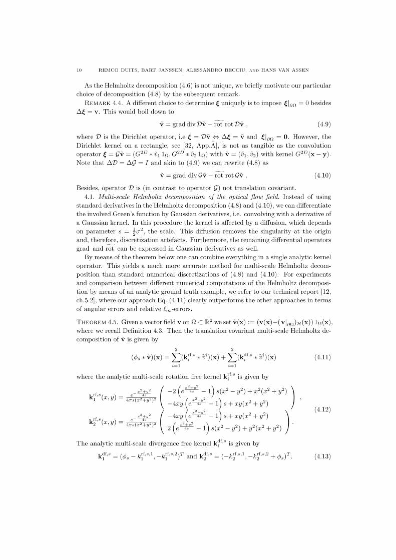
Theorem 4.5. Given a vector field v on Ω ⊂ R2 we set v(x) := (v(x)−(v|∂Ω)H(x)) 1Ω(x),where we recall Definition 4.3. Then the translation covariant multi-scale Helmholtz de-composition of v is given by
(φs ∗ v)(x) =2∑
i=1
(krf,si ∗ vi)(x) +
2∑
i=1
(kdf,si ∗ vi)(x) (4.11)
where the analytic multi-scale rotation free kernel krf,si is given by
krf,s1 (x, y) = e−
x2+y24s
4πs(x2+y2)2
−2
(e
x2+y2
4s − 1)
s(x2 − y2) + x2(x2 + y2)
−4xy(e
x2+y2
4s − 1)
s + xy(x2 + y2)
,
krf,s2 (x, y) = e−
x2+y24s
4πs(x2+y2)2
−4xy
(e
x2+y2
4s − 1)
s + xy(x2 + y2)
2(e
x2+y2
4s − 1)
s(x2 − y2) + y2(x2 + y2)
.
(4.12)
The analytic multi-scale divergence free kernel kdf,si is given by
kdf,s1 = (φs − krf,s,1
1 ,−krf,s,21 )T and kdf,s
2 = (−krf,s,12 ,−krf,s,2
2 + φs)T . (4.13)

MOTION ESTIMATION BY COVARIANT DERIVATIVES AND HELMHOLTZ DECOMPOSITION 11
Proof. Set G2Ds = φs ∗ G2D where φs denotes the heat kernel given in Eq. (3.1) and
G2D denotes the Green’s function given in Eq. (4.7). The diffused first order derivative(with respect to x) of the Green’s function can be computed via:
∂xG2Ds (x) = F−1
((ω1, ω2) 7→ iω1
2π
∫∞s
exp(−t(ω21 + ω2
2)) dt)(x, y)
=∫∞
s
x exp(− x2+y2
4t )
8πt2 dt = x2π
1−exp(− x2+y2
4s )
x2+y2 , x = (x, y),(4.14)
where ω1 and ω2 denote the frequency variables, cf. [8, Eq.14]. Similarly, one has
∂yG2Ds (x) =
y
2π
1− exp(−x2+y2
4s )x2 + y2
. (4.15)
The Helmholtz decomposition commutes with the diffusion operator and we expressboth the divergence and gradient operator by Gaussian derivatives in (4.10) where wecan exploit the semigroup property of diffusion: φs = φ s
2∗φ s
2. For the rotation free part
we get
∇( s2 ) div ( s
2 ) G v =2∑
i=1
(∇∂xiGs2D ∗ vi)(x)
=2∑
i=1
(krf,si ∗ vi)(x) :=
2∑i=1
((krf,s,1i ∗ vi)(x), (krf,s,2
i ∗ vi)(x))T ,
with x1 = x, x2 = y, with krf,si = ∇∂xiGs
2D and where e.g. ∇( s2 ) denotes the Gaussian
gradient at scale s2 , i.e. ∇( s
2 )f = ∇(φ s2∗ f) = (∇φ s
2∗ f). Finally, regarding the identity
(4.13) we note that φs ∗ v = ∇( s2 ) div ( s
2 )Gv− rot( s
2 ) rot ( s2 )Gv. ¤
Remark 4.6. In our algorithm the kernels krf,si and kdf,s
i are analytically precomputedfor a range of scales (according to the scale of the involved velocity features, cf. Section 3)via Eq. (4.12) and Eq. (4.13). The diffusion takes care of the singularities present at s = 0:The kernels krf,s
i and kdf,si are non-singular iff s > 0.
krf,s1 krf,s
2 kdf,s1 kdf,s
2
Fig. 6. Effective kernels of the multi-scale Helmholtz decomposition(4.11) at a fixed scale s > 0. Top row: first component of respec-
tively from left to right krf,s1 ,krf,s
2 ,kdf,s1 ,kdf,s
2 . Bottom row: second
component of respectively from left to right krf,s1 ,krf,s
2 ,kdf,s1 ,kdf,s
2 .
12 REMCO DUITS, BART JANSSEN, ALESSANDRO BECCIU, AND HANS VAN ASSEN
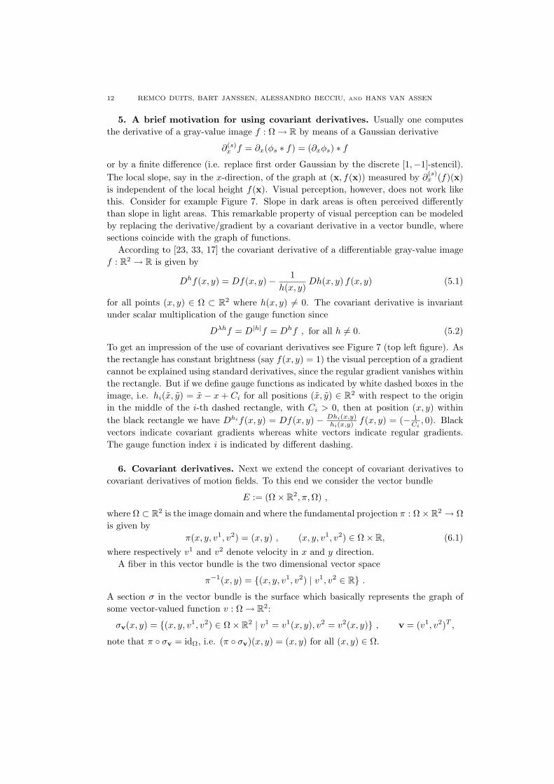
5. A brief motivation for using covariant derivatives. Usually one computesthe derivative of a gray-value image f : Ω → R by means of a Gaussian derivative
∂(s)x f = ∂x(φs ∗ f) = (∂xφs) ∗ f
or by a finite difference (i.e. replace first order Gaussian by the discrete [1,−1]-stencil).The local slope, say in the x-direction, of the graph at (x, f(x)) measured by ∂
(s)x (f)(x)
is independent of the local height f(x). Visual perception, however, does not work likethis. Consider for example Figure 7. Slope in dark areas is often perceived differentlythan slope in light areas. This remarkable property of visual perception can be modeledby replacing the derivative/gradient by a covariant derivative in a vector bundle, wheresections coincide with the graph of functions.
According to [23, 33, 17] the covariant derivative of a differentiable gray-value imagef : R2 → R is given by
Dhf(x, y) = Df(x, y)− 1h(x, y)
Dh(x, y) f(x, y) (5.1)
for all points (x, y) ∈ Ω ⊂ R2 where h(x, y) 6= 0. The covariant derivative is invariantunder scalar multiplication of the gauge function since
Dλhf = D|h|f = Dhf , for all h 6= 0. (5.2)
To get an impression of the use of covariant derivatives see Figure 7 (top left figure). Asthe rectangle has constant brightness (say f(x, y) = 1) the visual perception of a gradientcannot be explained using standard derivatives, since the regular gradient vanishes withinthe rectangle. But if we define gauge functions as indicated by white dashed boxes in theimage, i.e. hi(x, y) = x − x + Ci for all positions (x, y) ∈ R2 with respect to the originin the middle of the i-th dashed rectangle, with Ci > 0, then at position (x, y) withinthe black rectangle we have Dhif(x, y) = Df(x, y) − Dhi(x,y)
hi(x,y) f(x, y) = (− 1Ci
, 0). Blackvectors indicate covariant gradients whereas white vectors indicate regular gradients.The gauge function index i is indicated by different dashing.
6. Covariant derivatives. Next we extend the concept of covariant derivatives tocovariant derivatives of motion fields. To this end we consider the vector bundle
E := (Ω× R2, π, Ω) ,
where Ω ⊂ R2 is the image domain and where the fundamental projection π : Ω× R2 → Ωis given by
π(x, y, v1, v2) = (x, y) , (x, y, v1, v2) ∈ Ω× R, (6.1)
where respectively v1 and v2 denote velocity in x and y direction.A fiber in this vector bundle is the two dimensional vector space
π−1(x, y) = (x, y, v1, v2) | v1, v2 ∈ R .
A section σ in the vector bundle is the surface which basically represents the graph ofsome vector-valued function v : Ω → R2:
σv(x, y) = (x, y, v1, v2) ∈ Ω× R2 | v1 = v1(x, y), v2 = v2(x, y) , v = (v1, v2)T ,
note that π σv = idΩ, i.e. (π σv)(x, y) = (x, y) for all (x, y) ∈ Ω.

MOTION ESTIMATION BY COVARIANT DERIVATIVES AND HELMHOLTZ DECOMPOSITION 13
Fig. 7. Top row: The visual illusion on the left illustrates that dueto surrounding gray-values a slope is perceived in the rectangle, al-though the rectangle has constant brightness. The visual illusionon the right illustrates the opposite dependence: due to differentsurrounding slopes the same brightness is perceived differently (thediagonals appear brighter). Bottom row: The left visual illusion canbe modeled by covariant derivatives.
6.1. Connections on the Vector Bundle E. A connection on a vector bundle is bydefinition a mapping D : Γ(E) → L(Γ(T (Ω)),Γ(E)) from the space of sections in thevector bundle Γ(E) to the space of linear mappings L(Γ(T (Ω)),Γ(E)) from the spaceof vector fields on Ω denoted by Γ(T (Ω)) into the space of sections Γ(E) in the vectorbundle E such that
Dv+wσ = Dvσ + Dwσ , Dfvσ = fDvσ ,
Dv(σ + τ) = Dvσ + Dvτ , Dv(fσ) = v(f)σ + fDvσ(6.2)
for all vector fields v =∑2
i=1 vi∂xi ,w =∑2
i=1 wi∂xi ∈ Γ(T (Ω)) (i.e. sections in tangentbundle T (Ω)) and all f ∈ C∞(Ω,R) and all sections σ ∈ Γ(E) in the vector bundle E.We used the common short notation Dvσ = (Dσ)(v). Now Eq. (6.2) implies that
((Dσv)(X))(c(t)) = D(v1σ1 + v2σ2)(X)(c(t))
=2∑
j=1
X|c(t) (vj) σj +2∑
j=1
2∑i=1
vj(c(t)) ci(t) (D∂xi σj)(c(t)),(6.3)
where σ1(x, y) = (x, y, 1, 0) and σ2(x, y) = (x, y, 0, 1) denote the unit sections in x andy-direction and where X|c(t) =
∑2i=1 ci(t) ∂xi |c(t) denotes a vector field on Ω tangent to
a curve c : (0, 1) → Ω in the image domain Ω ⊂ R2.By Eq. (6.3) the connection D is uniquely determined by D∂xi σji,j=1,2. Now for
each i, j = 1, 2 this output D∂xi σj is a section and consequently there exist unique
functions Γkij : Ω → R (Christoffel-symbols) such that (D∂xi σj)(c(t)) =
2∑k=1
Γkij(c(t))σk .

14 REMCO DUITS, BART JANSSEN, ALESSANDRO BECCIU, AND HANS VAN ASSEN
Here we restrict ourselves to the diagonal case w.r.t. Euclidean coordinates
Γkij = Aj
i δkj , with Ak
i := Γkik . (6.4)
We impose this restriction for pragmatic reasons: It is a straightforward generalization ofour previous work on reconstruction of scalar valued functions using covariant derivatives[33]. Although this choice does not affect the rules for covariant derivatives on a vectorbundle (6.2). However, when using such derivatives in a velocity reconstruction, we willhave to check the rotation covariance of the algorithm.
6.2. Covariant derivatives on the Vector Bundle E induced by gauge fields. By ourrestriction (6.4) the covariant derivatives in E are given by
D∂xiσv = (Dσv)(∂xi) = (∂xiv1 + A1i v1)σ1 + (∂xiv2 + A2
i v2) σ2 (6.5)
with v =2∑
i=1
viσi ∈ Γ(E). Now we choose Aji such that an a priori given section σh (a
so-called gauge-field, [33]) (x, y) 7→ σh(x, y) with σh(x, y) = (x, y, h1(x, y), h2(x, y)) ,h =(h1, h2)T , is not affected (“invisible”) by the covariant derivative, i.e. we must solve for
(Dσh)(∂xi) = 0 ⇔ (∂xih1 + A1i h
1) σ1 + (∂xih2 + A2i h
2) σ2 = 0 σ1 + 0 σ2
⇔ Aji = −∂xihj
hj , for all i, j = 1, 2,(6.6)
so that the covariant derivative Dh induced by gauge-field σh ∈ Γ(E) is given by
(Dh∂xiσv)(x) = ((∂xi)h1v1)(x)σ1 + ((∂xi)h2v2)(x)σ2 ,
where we use short notation
(∂xi)hj
vj =∂vj
∂xi−
∂hj
∂xi
hjvj , for j = 1, 2. (6.7)
See Figure 8 for a geometrical interpretation of covariant derivatives, where for the sakeof illustration we consider the subset E0 := (x, y, v1, v2) ∈ E | v2 = 0 of the total vectorbundle consisting of all elements for which the fourth component vanishes and where boththe Gauge field σh and the velocity field σv are of the form σv(x, y) = (x, y, f(x), 0).
Remark 6.1. We consider the vector bundle E := (Ω × R2, π, Ω) with connectionD. One could also consider a tangent bundle (Ω, T (Ω)) equipped with a Levi-Cevitaconnection ∇ induced by some (image dependent) metric g. These connections could becombined in a tensor product ∇ ⊗ D which requires cumbersome bookkeeping. In [17]they are combined via new connection components Dmvj = ((∂m + Ai
m) δji + Γj
im)vi,where Γj
mi denote Christoffel symbols w.r.t. ∇ and where the flat case corresponds to(6.4). In any case (flat or non-flat ∇) we need to check whether the overall velocityreconstruction algorithm described in Fig. 2 is covariant with respect to rotations andtranslations acting simultaneously on the reconstructed field and the gauge field, as thisis not a priori guaranteed.
MOTION ESTIMATION BY COVARIANT DERIVATIVES AND HELMHOLTZ DECOMPOSITION 15
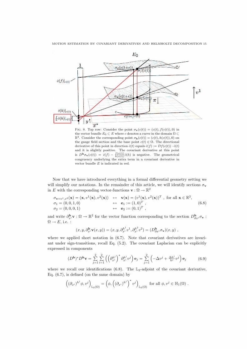
Fig. 8. Top row: Consider the point σv(c(t)) = (c(t), f(c(t)), 0) inthe vector bundle E0 ⊂ E where c denotes a curve in the domain Ω ⊂R2. Consider the corresponding point σh(c(t)) = (c(t), h(c(t)), 0) onthe gauge field section and the base point c(t) ∈ Ω. The directionalderivative of this point in direction c(t) equals c(f) := Df(c(t)) · c(t)and it is slightly positive. The covariant derivative at this point
is Dhσv(c(t)) = c(f) − f(c(t))h(c(t))
c(h) is negative. The geometrical
congruency underlying the extra term in a covariant derivative invector bundle E is indicated in red.
Now that we have introduced everything in a formal differential geometry setting wewill simplify our notations. In the remainder of this article, we will identify sections σv
in E with the corresponding vector-functions v : Ω → R2
σv=v1,v2(x) = (x, v1(x), v2(x)) ↔ v(x) = (v1(x), v2(x))T , for all x ∈ R2,
σ1 = (0, 0, 1, 0) ↔ e1 := (1, 0)T ,
σ2 = (0, 0, 0, 1) ↔ e2 := (0, 1)T ,
(6.8)
and write ∂hxiv : Ω → R2 for the vector function corresponding to the section Dh
∂xiσv :Ω → E, i.e. :
(x, y, ∂hxiv(x, y)) = (x, y, ∂h1
xi v1, ∂h2
xi v2) = (Dh∂xiσv)(x, y) ,
where we applied short notation in (6.7). Note that covariant derivatives are invari-ant under sign-transitions, recall Eq. (5.2). The covariant Laplacian can be explicitlyexpressed in components
(Dh)∗Dhv =2∑
j=1
2∑i=1
((∂hj
xi
)∗∂hj
xi vj)ej =
2∑j=1
(−∆vj + ∆hj
hj vj)ej (6.9)
where we recall our identifications (6.8). The L2-adjoint of the covariant derivative,Eq. (6.7), is defined (on the same domain) by
((∂xi)hj
φ, vj)L2(Ω)
=(φ,
((∂xi)hj
)∗vj
)L2(Ω)
for all φ, vj ∈ H1(Ω) .

16 REMCO DUITS, BART JANSSEN, ALESSANDRO BECCIU, AND HANS VAN ASSEN
Integration by parts yields
((∂xi)hj
)∗vj = −∂vj
∂xi−
∂hj
∂xi
hjvj . (6.10)
If we compare the adjoint covariant derivative to the covariant derivative we see thatthe multiplicator part is maintained whereas the derivative-part contains an extra minussign, cf. [17] that is missing in [23, Eq.21]. By straightforward computation one finds thefundamental formula:
−∆hj
vj :=2∑
i=1
(∂hj
xi
)∗∂hj
xi vj =2∑
i=1
− ∂∂xi
(∂
∂xi
)hj
vj −∂hj
∂xi ( ∂∂xi )
hj
vj
hj
=2∑
i=1
− ∂∂xi
(∂vj
∂xi − ∂hj
∂xivj
hj
)−
∂vj
∂xi
(∂vj
∂xi − ∂hj
∂xivj
hj
)
hj
= −∆vj + ∆hj
hj vj .
(6.11)
Now that we have introduced the covariant Laplacian we mention two preliminary issuesthat directly arise from (6.11) and which will be addressed in the remainder of this article.
Remark 6.2. At first sight the covariant derivatives and their associated (inverse)Laplacian, seem to be ill-posed as the gauge-field components should not vanish. How-ever, the crucial scaling property of covariant derivatives, Eq. (5.2) allows us to scaleaway from 0. Furthermore, as we will see later in Section 7 the Dirichlet kernel operatorof the coercive covariant Laplacian is stable. Finally, we will show how the manifeststability of our algorithms depends on the choice of gauge field.
6.3. Interpolation between conventional derivatives and covariant derivatives. A mono-tonic transformation on the components of the gauge field takes care of the interpolationbetween standard derivatives and covariant derivatives. For the sake of illustration werestrict ourselves to the scalar valued case (with positive gauge function h : Ω → R+,recall (5.2)) as the vector valued case follows by applying everything on the two separatecomponents. By applying a monotonic transformation h 7→ hη on the gauge function weobtain the following covariant derivative
Dhη
f = Df −D(log hη)f = Df − η(D log h)f . (6.12)
If η = 0 the expression (6.12) provides a conventional derivative, whereas the case η = 1yields a covariant derivative with respect to gauge function h. For further motivationand experiments on the choice of η we refer to our technical report [12, ch:10, Fig.15].
7. Fundamental properties of the self-adjoint covariant Laplacian. In thissection we shall show that the covariant Laplacian has more or less the same fundamen-tal properties as the ordinary Laplacian. These basic fundamental properties includingself-adjointness, negative definiteness, and coercivity are important for well-posed sym-metric inverse problems that shall arise from Euler Lagrange equations for vector fieldinterpolation later on in Section 9 and Section 11.
Definition 7.1. Let H be a Hilbert space with inner product (·, ·). An unboundedoperator A : H → H on a Hilbert space H with domain D(A) is self-adjoint if
(Af, g) = (f, Ag) for all f, g ∈ D(A) ,

MOTION ESTIMATION BY COVARIANT DERIVATIVES AND HELMHOLTZ DECOMPOSITION 17
and if the domain of the adjoint D(A∗) coincides with the domain of A, i.e. D(A∗) =D(A). Such an operator is coercive if there exists a positive constant c > 0 s.t.
(Af, f) ≥ c (f, f) for all f ∈ D(A).
Now suppose that the gauge field is twice continuously differentiable and |hj | > 0.By (5.2) we can assume that the components hj of the gauge field are positive, hj > 0.
The covariant Laplacian ∆hj
:= − ∑i=1,2
(∂hj
xi
)∗∂hj
xi is just like the ordinary Laplacian an
unbounded negative definite operator on L2(Ω) with domain
D(−∆hj
)= H0
2(Ω) := f ∈ H2(Ω) : f |∂Ω = 0. (7.1)
The covariant Laplacian operator ∆hj
is negative definite(−∆hj
f, f)L2(Ω)
=(∂hj
xi f, ∂hj
xi f)L2(Ω)
> 0
for all j = 1, 2 and all f 6= 0 regardless the choice of hj . The functions qj := ∆hj
hj arecontinuous on the compact domain Ω, so there exists some xj
0,yj0 ∈ Ω such that
∆hj(yj0)
hj(yj0)
≤ qj :=∆hj
hj≤ ∆hj(xj
0)hj(xj
0). (7.2)
Now minus the covariant Laplacian is a Sturm-Liouville operator [28]. Consequently, thecovariant Laplacian is self-adjoint and the corresponding self-adjoint resolvent operator
(I −∆hj
)−1
(7.3)
is compact and thereby there exists a complete orthonormal set of strictly positive eigen-values and eigenfunctions [50, Thm 13.33] such that
−∆hj
f jn = λj
nf jn , j = 1, 2,
f jn
∣∣∂Ω
= 0, j = 1, 2,⇔
−∆(f jn) + qj f j
n = λjnf j
n, j = 1, 2,
f jn
∣∣∂Ω
= 0, j = 1, 2,
where we stress that λn = 0 would yield the trivial solution only, as Dhj
f j = 0 impliesf j = λhj which for λ 6= 0 would contradict (7.2) since f j
n
∣∣∂Ω
= 0. Now the resolvent ofthe covariant Laplacian is compact with a domain H0
2(Ω) that is compactly embeddedin L2(Ω) and consequently, 0 is the only density point of the spectrum of the resolvent.Consequently, the spectrum of the minus covariant Laplacian is contained in
σ(−∆hj
)⊂ [ch(Ω),∞)
for some ch(Ω) > 0 and by the Sturm-Liouville theory [25] the spectrum only consistsof eigenvalues so that ch(Ω) equals the smallest eigenvalue λj
1 of −∆hj
restricted to itsdomain (7.1) which can be expressed by the Rayleigh quotient
λj1 = min
f∈H02(Ω)
∫Ω−f(x)∆f(x)+qj(x)|f(x)|2 dx
∫Ω|f |2(x)dx
= minf∈H0
2(Ω)
∫Ω
(∇f ·∇f)(x)+qj(x)|f(x)|2 dx
∫Ω|f(x)|2dx .
We conclude that the covariant Laplacian is just like the regular Laplacian a coerciveoperator on the domain H0
2(Ω) with a complete orthogonal basis of eigenfunctions. Thiscoercivity is important for the stability of the numerical algorithms (via the Lax-Milgram

18 REMCO DUITS, BART JANSSEN, ALESSANDRO BECCIU, AND HANS VAN ASSEN
theorem, [45]) later on, since inverting the covariant Laplacian boils down to invertingall the eigenvalues. In general it is apparent from the essential formula (6.11), that themore convex the gauge field, the more well-posed the inversion of the covariant Laplacianand the covariant resolvent (7.3) is. See Example 7.2 and Example 7.3 below, where werespectively consider basic gauge functions that are convex and concave. As the covariantLaplacian (6.11) of a vector field acts componentwise, we will consider examples of acovariant Laplacian
−∆hf = (Dh)∗Dhf = −∆f +∆h
hf
of a scalar field f with respect to a scalar field h.Example 7.2. Consider the case where Ω = [0, 1] × [0, 1] and h(x, y) = β eγ1x+γ2y,
with β ∈ R and β 6= 0, λi ∈ R, then∆h
h= |γ|2 = (γ1)2 + (γ2)2 ≥ 0
and we have (Dh)∗Dh = −∆+ |γ|2 I. The smallest eigenvalue of the covariant Laplacianequals 2π2 + γ2, which shows that the covariant Dirichlet problem is better posed thana regular Dirichlet problem in case of a convex gauge function h.
Example 7.3. Consider the case where Ω = [0, 1] × [0, 1] and the gauge function is
a Gaussian kernel h(x, y) = β( 12πσ2 e−
(x2+y2)2σ2 ), with β > 0 arbitrary. Set α := 1
2σ2 = 38 ,
then we end up with an extreme case where the gauge function is concave on the wholedomain Ω. A brief computation yields q(x, y) = ∆h(x,y)
h(x,y) = 4α(α(x2 + y2) − 1) andapplication of the method of separation (where we set f(x, y) = Xm(x)Yn(y)) to theeigenvalue problem (−∆ + q)f = λmnf with f |∂Ω = 0, yields
µm1 + µn
2 − 4α =4α2x2Xm(x)−X ′′
m(x)Xm(x)
− 4α2y2Yn(y)− Y ′′n (y)
Yn(y)− 4α = λmn (7.4)
with Xm(0) = Xm(1) = 0 and Yn(0) = Yn(1) = 0 and where µm1 , µn
2 , λmn are sepa-ration constants, all defined by (7.4). So set Xm(x) = e−αx2
Xm(2√
αx) and Yn(y) =e−αy2
Yn(2√
αy) and set ξ = 2x√
α and η = 2y√
α then we arrive at the Hermite differ-ential equation
X ′′m(ξ)− 2ξX ′
m(ξ)− 12Xm(ξ) = −µ1
2αXm(ξ) ,
Xm(0) = Xm(2√
α) = Xm
(√32
)= 0
and an analogous Hermite differential equation for Yn(η). Now we arrive at the Her-mite polynomials Hm(x) of order m, where the lowest order that could possibly fitthe boundary conditions is m = 3. This gives µm
12α − 1
2 = 6 = 2n ⇒ µm1 = 13α and
the eigenfunction with smallest eigenvalue of the covariant Laplacian equals (x, y) 7→e−α(x2+y)2H3(−2
√αx)H3(−2
√αy) with eigenvalue λ = µ1 + µ2 − 4α = 22α = 8.25,
which is less than 2π2 but still sufficiently far from 0.
8. The Green’s function of the covariant Laplacian and an explicit coer-civity bound. In the general case, where h ∈ C2([0, 1] × [0, 1],R) is arbitrary, we canget a grip on the coercivity constant ch(Ω) by considering the Green’s function of thecovariant Laplacian. Here we employ the decomposition −∆f + ∆h
h f = (Dh)∗Dhf and

MOTION ESTIMATION BY COVARIANT DERIVATIVES AND HELMHOLTZ DECOMPOSITION 19
we partially follow Sturm-Liouville theory, which does not directly apply since h−1∆h
need not be positive. To obtain the coercivity constant for (Dh)∗Dh we may restrictourselves to the 1 dimensional case since
(−∆ +∆h
h)f = −∂2f
∂x2+
∂2h∂x2
hf − ∂2f
∂y2+
∂2h∂y2
hf =
2∑
i=1
(∂h
∂xi
)∗(∂h
∂xi
)f.
Thereby a lower-bound ch([0, 1]) on the 1D-covariant Laplacian
H20([0, 1]) 3 f 7→ Dhf = −f ′′ +
h′′
hf ∈ L2([0, 1]) ,
produces a lower-bound on the 2D-covariant Laplacian by means of the estimate1∫
0
1∫
0
∣∣∣∣∂hf(x, y)
∂x
∣∣∣∣2
dxdy ≥1∫
0
ch(·,y)([0, 1])
1∫
0
|f(x, y)|2 dxdy.
This lower bound on the spectrum of the 2D covariant Laplacian is given by
σ
(−∆ +
∆h
h
)> ch([0, 1]× [0, 1]) := min
x∈[0,1]ch(x,·)([0, 1])+ min
y∈[0,1]ch(·,y)([0, 1]). (8.1)
Therefore, in the remainder of this subsection and Appendix A we consider a 1D gaugefunction h : [0, 1] → R and f ∈ L2([0, 1]). For the sake of sober notation we omit thetildes and write h ∈ C2([0, 1]) with h > 0 and f ∈ L2([0, 1]).
Theorem 8.1. The Green’s function of the 1D covariant Laplacian f 7→ (Dh)∗Dhf =−f ′′ + h′′
h f is given by
kh(x, y) =h(x)h(y)Qh(1)
·
Qh(x)(Qh(1)−Qh(y)) for x ≤ y ,
Qh(y)(Qh(1)−Qh(x)) for x > y(8.2)
with Qh(x) :=x∫0
(h(v))−2 dv. The compact self-adjoint operator Kh : L2([0, 1]) → H20([0, 1])
Khf(x) =
1∫
0
kh(x, y)f(y) dy (8.3)
is the right-inverse of the covariant Laplacian
(Dh)∗DhKhf = f for all f ∈ L2([0, 1]). (8.4)
The operator norm of Kh can be estimated by the Hilbert-Schmidt norm
‖Kh‖ ≤ |||Kh||| =√
traceK∗hKh = ‖kh‖L2([0,1]2) ≤
√2‖h−1‖L2([0,1])‖h‖L2([0,1]) (8.5)
and we have the following lower bound for the spectrum of the 1D-covariant Laplacian
σ((Dh)∗Dh) ≥ 1|||Kh||| ≥ ch([0, 1]) ≥ 1√
2‖h−1‖−1
L2([0,1])‖h‖−1L2([0,1]) . (8.6)
and the following lower bound for the spectrum of the 2D-covariant Laplacianσ
(−∆ + ∆hh
) ≥ ch([0, 1]× [0, 1]) ≥ 1√2
minx∈[0,1]
‖h−1(x, ·)‖L2([0,1])‖h(x, ·)‖L2([0,1])
+ 1√2
miny∈[0,1]
‖h−1(·, y)‖L2([0,1])‖h(·, y)‖L2([0,1]) .(8.7)

20 REMCO DUITS, BART JANSSEN, ALESSANDRO BECCIU, AND HANS VAN ASSEN
The covariant Laplacian has a complete orthonormal basis of eigenfunctions and themaximum lower bound ch([0, 1]× [0, 1]) coincides with the smallest eigenvalue.
Proof. For the derivation of the main part of the theorem, that is Eq. (8.2), Eq. (8.4)and inequality (8.6), we refer to Appendix A. Furthermore, we rely on standard resultsfrom functional analysis such as the fact that every Hilbert Schmidt operator is compact,the Hilbert-Schmidt norm of a kernel operator Kh equals the L2-norm of its kernel h,the spectral decomposition theorem for compact self-adjoint operators, and the fact thatthe Hilbert-Schmidt norm is an upper bound of the operator norm. Note that bothoperator (Dh)∗Dh (unbounded on L2([0, 1])) and operator Kh are self-adjoint (withkh(x, y) = k(y, x)) and by the spectral decomposition theorem for compact self-adjointoperators they share a common orthonormal basis of eigenfunctions from which the resultfollows. Finally, the lower-bound (8.7) follows by Eq. (8.6) and Eq. (8.1). ¤In Figure 9 we have plotted the graphs of Green’s functions x 7→ kh(x, y) of the covariantLaplacian for various gauge functions h : [0, 1] → R and several y ∈ [0, 1].
Fig. 9. The graphs of gauge functions h and the correspondingGreen’s functions kh(·, y) of the covariant Laplacian (where delta-spikes are respectively placed at y = 0.25, 0.5, 0.75). In red: gaugefunction of Example 7.2 (convex case, γ = 3). In blue: gauge
function of Example 7.3 (concave case, σ = 14
√3). In dashed
black: Green’s function with respect to constant gauge functions(i.e. Green’s function of standard Laplacian). The Green’s functionis convex (concave) if the gauge field is convex (concave).
Remark 8.2. The lower-bounds in the estimates (8.6), (8.7) explicitly depend on thegauge field, but they need not be sharp. The invariance with respect to scaling of thegauge function
(Dh)∗Dh = (Dλh)∗Dλh and Kh = Kλh and ch = cλh, λ 6= 0,
is also reflected in the estimate (8.7) as it should.Finally, we note the following result (which can also be observed in Figure 9).
Lemma 8.3. if the gauge function h > 0 is convex (respectively concave) then the corre-sponding Green’s function k(·, y) = ((Dh)∗Dh)−1δy of the covariant Laplacian is convex(respectively concave) as well.
For a proof of this result, see the last paragraph of Appendix A.
MOTION ESTIMATION BY COVARIANT DERIVATIVES AND HELMHOLTZ DECOMPOSITION 21
9. Tikhonov regularized optic flow reconstruction expressed in covariantderivatives. In order to formulate Tikhonov regularization in covariant derivatives, wefirst have to derive a gauge field. Such a gauge field imposes an a priori balance betweenvelocity magnitude and velocity field changes and thereby it is supposed to be close tothe velocity field that we would like to reconstruct from a sparse set of features. Thereare several options to choose the gauge field as an initial guess for the velocity field. Wepropose the standard Tikhonov regularization reconstruction with standard derivatives(i.e. constant gauge field) as a gauge field for a subsequent Tikhonov regularizationreconstruction using covariant derivatives. The latter step is then to be considered as arefinement of the first.
Next we explain the whole reconstruction procedure in formulas. Subsequently, we willmotivate the use of covariant derivatives and we will solve and analyze the correspondingEuler-Lagrange equations.
Definition 9.1. Let Ω be an open, convex subset of R2 with a piecewise smoothboundary. Let k ∈ 1, . . . , K denote a fixed time frame and let λ > 0. Let wk
q NBq=1 ∈
(R+)NB denote a given weight vector. Let hk be a smooth gauge field on Ω and let thediscrete (sparse velocity) vector
dk := (dk,1,dk,2)T ∈ R2NB (9.1)
be given by dk,j := (dk,j1 , dk,j
2 , . . . , dk,jNB
)T ∈ RNB , with components given by Eq. (3.6).Let
φqk(x) := φsq(tk)(x− xq
s=sq(tk)) (9.2)
denote the Gaussian kernel, Eq. (3.1), centered around xqs=sq(tk) ∈ R2 with scale sq(tk) > 0,
recall Figure 5, such that
(φqk, vk,j)L2(Ω) = (φs=sq(tk) ∗ vkj)(xq
s=sq(tk)) = dk,jq , (9.3)
where q ∈ 1, . . . , NB enumerates the extremal branches and where j ∈ 1, 2 enumer-ates the vertical and horizontal component of the field.
Then we define the energy3 of a smooth velocity field vk on Ω by
Eλ,hk,dk
(vk) := λEhk
reg(vk) + Edk
data(vk) :=
λ∫Ω
|||Dhk
vk(x)|||2 dx +NB∑q=1
wkq
2∑j=1
|(φqk, vk,j)L2(Ω) − dk,j
q |2, (9.4)
where |||Dhk
vk(x)||| denotes the Hilbert-Schmidt norm of the tensor field Dhk
vk(x) =∑2i,j=1 ∂hk,j
xi vk,j(x) dxi ⊗ ∂j , i.e.:
|||Dhk
vk(x)|||2 =2∑
i=1
2∑
j=1
|∂hk,j
xi vk,j(x)|2 .
The reconstruction procedure is as follows. The velocity field vk = vk,1e1 +vk,2e2, attime-step k, is obtained by first minimizing Eλ,hk=1,dk
(vk) for hk = 1 is constant yieldingoptimal field say (vk)∗ which produces the gauge field hk := (vk)∗ for the second/final
3Later in Section 13 we propose a minor adaptation for a fully rotation covariant energy.
22 REMCO DUITS, BART JANSSEN, ALESSANDRO BECCIU, AND HANS VAN ASSEN
refinement step where Eλ,(vk)∗,dk
(vk) is minimized. Within each minimization, the pa-rameter λ > 0 balances between regularization part and the soft constraints weighted bywk
q > 0. In our algorithm we have set wkq = 1.
The minimization takes place over the space H10(Ω) = H1
0(Ω) × H10(Ω) so we shall
assume that v vanishes at the boundary. In practical applications where the field doesnot vanish at the boundary, we subtract the Harmonic infilling v = v− (v|∂Ω)H. In theremainder of this article we simply write v ∈ H1
0(Ω) instead of v ∈ H10(Ω).
For λ > 0 and hard-constraints (wkq → ∞) we arrive at the minimization framework
on a space of Sobolev-type, [11][ch:3.4.2.1], where we must set R = ((Dhk
)∗Dhk
+ I)12
to construct the complete Sobolev-space D(R) on which the minimization problem takesplace. The unique minimizer is then found by orthogonal projection. Variation of λ > 0can considerably improve the reconstruction, likewise Figure 4 (right column).
9.1. The advantage of covariant derivatives. By using covariant derivatives (w.r.t.gauge field (vk)∗), instead of regular derivatives, we employ the same velocity featurestwice; both in the data term and in the regularization term. The sparser the set offeatures, the more dominant the regularization term becomes. When using covariantderivatives w.r.t. gauge field (vk)∗ the regularization term prefers (fields close to) thegauge field (which is based on the features) over constant fields which are in general notbased on the features.
9.2. The Euler-Lagrange equations for the unique minimizer. Recall from Section 8that the covariant Laplacian (Dhk
)∗Dhk
: H20(Ω) → L2(Ω) is coercive. Thereby the
energy minimization problem (9.4) over the Hilbert space H20(Ω) (compactly and densely
embedded in L2(Ω)) consists (after diagonalization, Theorem 8.1) of a convex lower semi-continuous functional so that the existence and uniqueness of the minimizer is guaranteedby the general results in [15, Thm 1, p.524-526].
The Euler-Lagrange equation for the unique minimizer of (9.4) is derived by
limε→0
Eλ,hk,dk
(vk + εδ)− Eλ,hk,dk
(vk)ε
= 0 (9.5)
which is supposed to hold for all infinitely smooth perturbations that are compactlysupported within the interior of Ω, i.e. δ ∈ D(Ω).
Lemma 9.2. The Euler-Lagrange equation in the general continuous Tikhonov regular-ization framework using covariant derivatives (i.e. the minimization of Eq.(9.4)) is givenby
(λ (Dhk
)∗Dhk
+ S∗kΛkSk)vk = S∗kΛkdk (9.6)
where Sk : L2(Ω) → R2×NB is given by
(Skvk)(q) = (φqk,vk) := (φq
k, vk,1)L2(Ω)e1 + (φqk, vk,2)L2(Ω)e2 , (9.7)
and where Λk ∈ RNB×NB is the diagonal matrix consisting of the corresponding weights:
Λk = diagq=1...NB
(wkq ). (9.8)
Proof. Straightforward computation of (9.5) yields
∀δ∈D(Ω)2 ((λ (Dhk
)∗Dhk
)vk + S∗kΛkSkvk − S∗kΛkdk, δ) = 0

MOTION ESTIMATION BY COVARIANT DERIVATIVES AND HELMHOLTZ DECOMPOSITION 23
from which the result follows. ¤The adjoint S∗k : R2×NB → L2(Ω) operator for each fixed discrete time k ∈ N is definedby
(S∗kΦ,vk)L2(Ω) = (Φ,Skvk)R2×NB
and by straightforward manipulation (see [12, ch:8,p.24]) we find
(S∗kΦ)(x) =2∑
j=1
ej
(NB∑q=1
(Φ(q))jφqk(x)
). (9.9)
This allows to write down the Euler-Lagrange equations (9.6) in more explicit form:
NB∑q=1
wkq
((φq
k, vk,j)L2(Ω) − dk,jq
)φq
k(x)
+λ(−∆|vk,j |(x) + η ∆|hk,j |(x)
|hk,j |(x)vk,j(x)
)= 0
(9.10)
for j = 1, 2, x ∈ R2, with η = 1. Recall from Section 6.3 that we can interpolatebetween regular and covariant derivatives by varying the parameter η ∈ [0, 1]. We willuse Eq. (9.10) as a starting point for our implementations where all field components areexpanded in a B-spline basis. For stability analysis we prefer the more structured form(9.6) where the whole operator is bounded from below (by the results in Section 7 & 8)so that
((λ (Dhk
)∗Dhk
+ S∗kΛkSk)v,v)L2(Ω) > c(Ω) λ(v,v)L2(Ω)
and thereby operator λ (Dhk
)∗Dhk
+S∗kΛkSk is invertible. Summarizing, we have provedthe following result:
Theorem 9.3. The unique minimizer of the minimization problem (9.4) is given by
vk = (λ (Dhk
)∗Dhk
+ S∗kΛkSk)−1S∗kΛk dk , (9.11)
where Sk : L2(Ω) → R2×NB is given by Eq. (9.7), S∗k is given by Eq. (9.9), Λk given byEq. (9.8) and dk given by Eq. (9.1) and Eq. (9.3).
10. Reconstruction Algorithm: Solving the Euler-Lagrange Equations byExpansion in B-splines. Next we express the Euler-Lagrange equations entirely inB-spline coefficients. The computational advantages of using B-splines for variationalapproaches are well-known in signal in image processing, [21, 31, 57]. We will firstprovide a few basic properties on B-splines that we will need for our algorithm and theanalysis of its stability later on.
The n-th order (centered) B-spline is given by (n − 1)-fold convolution of B0 withitself
Bn(x) =(B0 ∗n−1 B0
)(x) with B0(x) = 1[− 1
2 , 12 ](x) , (10.1)
where (f ∗ g)(x) =∫∞−∞ f(y)g(x − y)dy. Thereby the n-th order B-spline is compactly
supported on 1[−n2− 1
2 , n2 + 1
2 ]. In the discrete setting we sample on a uniform integer grid,

24 REMCO DUITS, BART JANSSEN, ALESSANDRO BECCIU, AND HANS VAN ASSEN
so for example if n is odd we find n non-zero-samples. The regular derivative of a B-splineof order n is expressed in B-splines of order n− 1
d
dxBn(x) = Bn−1(x + 1/2)−Bn−1(x− 1/2).
Consequently, for even order derivatives of B-splines we have
(Bn)(2k)(x) =k∑
l=−k
(−1)l
(k
|l|)
Bn−2k(x− l) .
Next we express the unknown velocities vk,j : Ω → R, j = 1, 2, at time-frame t = k∆t,in periodic B-splines
vk,j(x, y) =L−1∑l=0
M−1∑m=0
ck,jlm bml(x, y) , with
bml(x, y) = Bn(
xa −m Mod M
a
)Bn
(yb − l Mod L
b
),
(10.2)
for all (x, y) ∈ Ω = [0,M ]× [0, L], where the field vk = vk−(vk
∣∣∂Ω
)H is indeed periodic.
In our algorithms we set the resolution parameters a = b = 1. One can choose themdifferently, as in [31], provided that the n-th order B-splines are properly sampled on[0,M ]× [0, L], i.e.
M
a> n + 1 and
L
b> n + 1 . (10.3)
Definition 10.1. We define the discrete energy corresponding to the continuous en-ergy Eλ,hk,dk(vk) given in Definition 9.1 by
Eλ,hk,dk(ck,dk) := Eλ,hk,dk(vk). (10.4)
where vk is expanded in the B-spline basis (10.2) and where
ck = ((ck,1)T , (ck,2)T )T =(ck,111 , ck,1
12 , . . . , ck,11M , ck,1
21 , ck,122 , . . . , ck,1
2M , . . . , . . . , ck,1L1 , ck,1
L2 , . . . , ck,1LM ;
ck,211 , ck,2
12 , . . . , ck,21M , ck,2
21 , ck,222 , . . . , ck,2
2M , . . . , . . . , ck,2L1 , ck,2
L2 , . . . , ck,2LM
)T
∈ R2ML
(10.5)
Lemma 10.2. Let k ∈ 1, . . . , K be a given time frame index. The discrete energy attime k∆t can be expressed directly in the B-spline coefficients:
Eλ,hk,dk(ck,dk) :=2∑
j=1
(ckj , Rλk,jc
kj)`2(1,...,LM) + ‖Λ1/2k (Sck,j − dk,j)‖2`2(1,...,NB) ,
(10.6)where the RML×ML matrices Rλ
k,j , for j = 1, 2 are given by
Rλk,j = λ(−TL,0(y
b )⊗ TM,2(xa )− TL,2(y
b )⊗ TM,0(xa )
+λM−1∑x=0
L−1∑y=0
γk,j(x, y)(TL,0(yb )⊗ TM,0(x
a ))(10.7)

MOTION ESTIMATION BY COVARIANT DERIVATIVES AND HELMHOLTZ DECOMPOSITION 25
where (ck,j , RL,0⊗RM,0ck,j) =L−1∑l,l′=0
M−1∑m,m′
ck,jlm ck,j
l′m′(RL,0)ll′(RM,0)mm′ and A⊗B denotes
the Kronecker product of matrices and where
TP,k(u) = [T pp′
P,k(u)] ∈ RP×P with T pp′
P,k(u) := (Bn)(k)(u− p)Bn(u− p′),TP,k = [T pp′
P,k ] ∈ RP×P with T pp′
P,k := (B2n)(k)(p− p′ Mod P ),(10.8)
with p, p′ ∈ 1, . . . , P, P ∈ L,M. The functions γk,j : Ω → R are given by
γk,j(x, y) =∆hk,j(x, y)hk,j(x, y)
= −∆(− log |hk,j |)(x, y) + ‖∇ log |hk,j |(x, y)‖2 .
Proof. By property (10.1) and assuming (10.3) we have the following formula for thecomponents T pp′
PK of the rank-2 tensor TP,K on RP :
T pp′
P,k := 1a
∫ P
0(Bn)(k)(x
a − p Mod Pa ) Bn(x
a − p′ Mod Pa ) dx
= 1a
∫ P2
−P2(Bn)(k)(x
a − p Mod Pa ) Bn(x
a − p′ Mod Pa ) dx
= (B2n)(k)(p− p′ Mod P ) ,
with P ∈ M,L. The matrix representation of the covariant Laplacian expressed in theB-spline basis is given by
Rλk,j = λ(−TL,0(y
b )⊗ TM,2(xa )− TL,2(y
b )⊗ TM,0(xa )
+λM−1∑x=0
L−1∑y=0
γk,j(x, y)(TL,0(yb )⊗ TM,0(x
a ))(10.9)
where (ck,j , RL,0⊗RM,0ck,j) =L−1∑l,l′=0
M−1∑m,m′
ck,jlm ck,j
l′m′(RL,0)ll′(RM,0)mm′ and A⊗B denotes
the Kronecker product of matrices. The rest follows by direct computation [12]. ¤Next we derive the discrete analogue of Lemma 9.2. To this end we express the mappingS in (9.7) in B-spline coefficients ck:
Skck(q) =2∑
j=1
ej
(L−1∑
l=0
M−1∑m=0
ck,jlm
(φq
k , bml))
.
If we expand the feature vectors φqkNB
q=1 as well φqk =
∑M−1m′=1
∑L−1l′=0 ck,q
l′m′bm′l′ , then wemay rewrite the mapping Sk : R2LM → Rq as
Skck(q) =L−1∑l,l′=0
M−1∑m,m′=0
ckqlm′Tmm′
M,0 T ll′L,0c
kjlm = (ckq)T (TL,0 ⊗ TM,0) ckj .
Theorem 10.3. Let the order n of B-spline basis n ≤ 3. Then the unique minimizer ofthe discrete functional (10.6) is given by
ck,j = (Rλk,j + ST
k ΛkSk)−1STk Λkdk,j , (10.10)
using the natural matrix-representation Sk ∈ RNB×LM of the isomorphic mappingsck1 7→ Sk(ck1,0) and ck2 7→ Sk(0, ck2).
Proof. To compute the unique minimizer we set ∇ckEλ,hk,dk(ck) = 0, yielding
(Rλk,j + ST
k ΛkSk)ck,j = STk Λkdk,j for j = 1, 2, (10.11)

26 REMCO DUITS, BART JANSSEN, ALESSANDRO BECCIU, AND HANS VAN ASSEN
with dk,j given by (9.1) and (9.3). The discrete system (10.11) minimizing the discretefunctional (10.6) is consistent with (9.11) minimizing the continuous functional (9.4).Its solution coincides with the unique solution of the continuous system if the velocitycomponents are constrained to the (closed) linear span
spanm=0,...,M−1,l=0,...,L−1
bml. (10.12)
For n ≤ 3, it will follow by the results in the next section (Corollary 11.2), that thesystem is well-posed and its unique solution is (akin to (9.11)) found by the inversion inEq. (10.10) and the result follows. ¤
Remark 10.4. We solved (10.10) by a BiGCSTAB algorithm, [51, ch:7.4.2]. Here wehave exploited the direct product structure of the terms in the matrix Rλ
k (10.9): Fornumerical efficiency one only needs to store the product M ×M or L×L matrices suchas TM,0 and TL,0 using the computation scheme explained in [27] in the BiGCSTABalgorithm whenever a matrix product occurs.
11. Stability Analysis of the Linear System in the Euler Lagrange Equa-tions. In this subsection we will analyze the stability of the inversion scheme (10.10)which is basically the matrix representation of operator equation (9.11) where we restrictourselves to the subspace (10.12). By Theorem 9.3 the continuous operator
λ (Dhk
)∗Dhk
+ S∗kΛkSk (11.1)
can be inverted in (9.11) and we have
λ (Dhk
)∗Dhk ≥ λ chk and S∗kΛkSk ≥ 0 ,
where chk is the Poincare constant of the covariant Laplacian, which depends on thechoice of gauge field hk. In practice (where gauge fields are convex in large subsets ofΩ) this Poincare constant is larger than the Poincare constant of the regular Laplacian,recall Example 7.3.
Let us return to the finite matrix representations Rλk,j + ST ΛkS, j = 1, 2 of operator
(11.1) with respect to the periodic B-spline basis (10.2), where we recall (10.9). We wouldlike to get estimates for the smallest eigenvalue of this finite matrix and we would like toinvestigate how this smallest eigenvalue depends on the order of the B-splines. First of allwe observe that the data matrix ST ΛkS ∈ RNB×LM is only positive semi -definite withLM À NB , so even in the case where all features are linearly independent we should notexpect global stability from the data matrix.
Lemma 11.1. Let the order n of B-splines be less or equal than 3. Let λ > 0, k ∈1, . . . ,K, j ∈ 1, 2. The real value of the eigenvalues of matrix Rλ
k,j is larger than
chkλ
(686323040
)2
> 0 ,
where chk > 0 denotes the Poincare constant of the covariant Laplacian on Ω, which isusually larger then the Poincare constant of the regular Laplacian on Ω (e.g. π2(M−2 + L−2)on a rectangle Ω = [0,M ]× [0, L]).

MOTION ESTIMATION BY COVARIANT DERIVATIVES AND HELMHOLTZ DECOMPOSITION 27
Proof. The regularization matrix Rλk,j for each component j ∈ 0, 1 satisfies
Rλk,j ≥ chk λ TL,0 ⊗ TM,0, (11.2)
with TL,0 and TM,0 given by Eq. (10.8), since substitution of (10.2) into (v,v)L2(Ω),Ω = [0,M ]× [0, L], gives
2∑j=1
(ckj , Rλk,jc
kj)`2(1,...,LM) = (λ (Dhk
)∗Dhk
v,v)L2(Ω) ≥
chk λ (v,v)L2(Ω) = chk λ2∑
j=1
(ckj , TL,0 ⊗ TM,0ckj)`2(1,...,LM) .
Now (11.2) relates the stability of matrix TL,0 ⊗ TM,0 with inverse (TL,0 ⊗ TM,0)−1 =T−1
L,0 ⊗ T−1M,0 to the stability of Rλk,j . The eigenvalues of TL,0 ⊗ TM,0 are direct products
of the eigenvalues of TL,0 with the eigenvalues of TM,0 so in order to find a lower-boundof the smallest eigenvalue of Rλ
k,j we derive the smallest eigenvalue of TP,0 with P ∈M,L. Now TP,0 = [TP,0]pp′ = [B2n(p − p′ Mod P )]pp′ is a circulant Toeplitz matrixwhose columns add up to one. This matrix is not symmetric (due to periodicity) so itseigenvalues need not be real-valued. It is positive definite though and since
(ckj , TL,0⊗TM,0ckj)`2(1,...,LM) = (ckj ,12(TL,0⊗TM,0+(TL,0⊗TM,0)T )ckj)`2(1,...,LM) ,
we only need to consider the real part of the eigenvalues Re(λ) = 12 (λ + λ). The Ger-
schgorin circle theorem [24] shows that the eigenvalues are contained within the circles
|λ−B2n(0)| ≤ 1−B2n(0) ⇔√|Re(λ)−B2n(0)|2 + |Im(λ)|2 ≤ 1−B2n(0) , (11.3)
where we note that 2B2n(0)−1 is strictly positive iff n ≤ 3. The eigenvalues of circulantToeplitz matrices can be computed explicitly (eigenvalues of a circulant Toeplitz matrixcoincide with the Discrete Fourier Transform (DFT) of the first row):
λp =P−1∑p′=0
B2n(p′)e−2πi p′p
P ,
Re(λp) = B2n(0) + 12 (ZB2n)(e
−2πi pP ) ,
(11.4)
with corresponding eigenvector (1, e−2πip
P , . . . , e−2πip(P−1)
P )T ∈ CP , p = 0, . . . , P −1. TheZ-transform of B2n is given by (ZB2n)(z) =
∑np′=−n c2n
p′ z−p′ , with c2n
p′ ∈ R+ monotoni-cally decreasing with c2n
0 = B2n(0) and as a result we can estimate the eigenvalues
B2n(0) +P−1∑
p′=1
(−1)p′c2np′ = Re(λp= P
2) ≤ Re(λp) ≤ Re(λ0) = 1.
The lower bound depends on n. Exact computations for n ≤ 10 indicate that it ismonotonically decreasing with n. We found 5
8 , 155384 , 6863
23040 ≈ 0.298, for n = 1, 2, 3. ¤
Corollary 11.2. The system in Theorem 10.3 is well-posed.
In our experiments we have set n = 3, M = L = 93 and λ = 100.06 ≈ 1.15 and we hadchk > π2(M−2 + L−2) ≈ 0.0023.

28 REMCO DUITS, BART JANSSEN, ALESSANDRO BECCIU, AND HANS VAN ASSEN
12. Algorithm. The overall algorithm combines(1) the sparse vector field obtained by scale selection of critical point velocities as
described in Section 3,(2) the multi-scale Helmholtz decomposition considered in Section 4, Theorem 4.5,(3) the Euler Lagrange equations of Tikhonov regularization expressed in covari-
ant derivatives as considered, analytically and numerically solved in respectivelySection 9, Theorem 9.3 and Section 10.
Recall Figure 2. We first compute the scale space representation (x, y, s, t) 7→ I(x, y, s, t),and the critical branches s 7→ (xq
s(t), s)NBq=1 therein, of the pre-processed tagged MRI-
images. For the critical branches we use a method based on winding numbers [53] forsub-pixel accuracy [12]. Then we determine the points (xs=sq(t), s
q(t)) on these branchesby means of the scale selection criterium (3.3). At these points we compute a sparse setof velocities dk
q and associated feature vectors φqk according to Eq. (3.5), (3.6), and (9.2).
This sparse set of velocities is distributed over the divergence and rotation free part asfollows. We apply a reconstruction by means of a Tikhonov regularization scheme withstandard derivatives and very small 0 < λ ¿ 1 to obtain a (full) regularized velocity fieldvk that (nearly) satisfies the hard constraints. Then we apply multi-scale Helmholtzdecomposition using the analytic vector-valued kernels from Theorem 4.5:
dk =((φsq(tk) ∗ vk)(xs=sq(t))
)q=1...NB
=((φsq(tk) ∗ vk,rf)(xs=sq(tk))
)q=1...NB
+((φsq(tk) ∗ vk,df)(xs=sq(tk))
)q=1...NB
=
(2∑
j=1
(krf,sq(tk)j ∗ vk,j)(xs=sq(tk))
)
q=1...NB
+
(2∑
j=1
(kdf,sq(tk)j ∗ vk,j)(xs=sq(tk))
)
q=1...NB
=: dk,rf + dk,df
(12.1)to split the sparse feature vector dk (cf. Eq. (9.1),(9.3) and (3.1)), at each time frame
tk = k∆t. This decomposition corresponds to the right most green box in Figure 2.Furthermore, the red boxes in Figure 2 correspond to minimizing the energy (9.4) inDefinition 9.1 by means of Eq. (9.11) in Theorem 9.3. More precisely, the red boxescorrespond to minimization of the discrete energy (10.6) in Definition 10.1 obtained byexpansion in a B-spline basis, solved by means of Eq. (10.10) in Theorem 10.3. The finalresult is obtained by adding the reconstruction from the divergence free gauge field hk,df
and dk,df to the reconstruction from the rotation free gauge field hk,rf and dk,rf.
13. Rotation covariance. Our algorithm commutes with translations, i.e. trans-lation of input image f : R2 × R+ → R results in a translated optical flow vector fieldv. With respect to rotations this commutation property is not a priori satisfied. Subse-quently, we show how to adapt the energy to obtain a fully rotation covariant algorithm.
Rotation of the input scalar field is given by f 7→ fR whereas rotation of the outputoptic flow vector field is given by vk 7→ vk
R, k = 1, . . . , K, where
fR(x, t) = f(R−1x, t) and vR(x, t) = Rv(R−1x, t) .
Our algorithm is rotation covariant if
Eλ,hkR,(Rdk
q )NBq=1(vk
R) = Eλ,hk,(dkq )
NBq=1(vk) (13.1)

MOTION ESTIMATION BY COVARIANT DERIVATIVES AND HELMHOLTZ DECOMPOSITION 29
for all R ∈ SO(2), k = 1, . . . , K. If R is a rotation over nπ/2, with n ∈ Z, then (13.1)is satisfied, see [12, ch.8.2]. For the other cases it depends on the spherical fluctuationsbetween the fraction of slope and height of the graph of the projected (gauge) field, whereprojections take place on each orientation n ∈ S2.
Strict rotation covariance is obtained by replacing Ehk
reg(vk), cf. Eq. (9.4), with
Ehk
reg(vk) =
∫ 2π
0
‖Dhk(x)·n(θ)(vk(x) · n(θ))‖2 dθ , (13.2)
with n(θ) = (cos θ, sin θ)T . In the algorithm this boils down to replacing
(Dhk
)∗Dhk
vk(x) =2∑
i,j=1
((∂
∂xi
)hk,j)∗ (
∂∂xi
)hk,j
vk,j(x) ej −→2π∫0
((Dhkθ )∗Dhk
θ vkθ )(x) n(θ) dθ =
2π∫0
(−∆vkθ (x) + ∆hk
θ (x)
hkθ (x)
vkθ (x)) n(θ) dθ
(13.3)
where vkθ := vk · n(θ) and hk
θ := hk · n(θ).Note that Ehk
reg(vk) is a course sampling of Ehk
reg(vk) (sampled at 0, π
2 , π, 3π2 ). Recall
Remark 6.1: For properly defined 2-tensors t on a circle one has∫ 2π
0t(n(θ),n(θ)) dθ =∑
k∈0,1 t(n(k π2 ),n(k π
2 )) = trace(t). However, a series of experiments in [12, Fig.12]show that Eq. (13.2) has a minor correcting effect and the replacement (13.3) is notneeded.
14. A single Euler Lagrange system involving covariant derivatives andHelmholtz decomposition. In this section we will consider a single Euler-Lagrangesystem involving both multi-scale Helmholtz decomposition and covariant derivatives.We will see direct analogy with our approach explained in Section 12 and Figure 2. Theapproach in this section has the advantage that it splits the divergence free and rotationfree part more consistently, although it is much more cumbersome to implement.
In the sequel we shall denote the divergence free part of the optical flow vector fieldvk at the kth time frame by vk,df and the rotation free part by vk,rf.
At a given fixed time frame t = k∆t we minimize the following positive functional
Eλ,hk,dk
(vk) :=∫Ω
λ |||D(hk)dfvk,df(x)|||2 dx +
∫Ω
λ |||D(hk)rfvk,rf(x)|||2 dx
+NB∑q=1
wkq
2∑j=1
|(φqk, vk,j)L2(Ω) − dk,j
q |2
+
(14.1)
where ||| · ||| denotes the Hilbert-Schmidt norm, and where we recall the previous def-initions in Section 9. We again first consider the simple case hk = (1, 1)T (where allcovariant derivatives become standard derivatives) to construct our gauge field hk.
Theorem 14.1. The unique minimizer v = vk at the k-th time frame of the problem
minv ∈ H1
0(Ω),
s.t. vdf∣∣∣∂Ω
= vrf∣∣∣∂Ω
= 0
Eλ,hk,dk
(v),

30 REMCO DUITS, BART JANSSEN, ALESSANDRO BECCIU, AND HANS VAN ASSEN
with positive, convex functional given by Eq. (14.1), is given by vk = ∇φ + rotA whereφ ∈ H2
0(Ω) is the unique weak solution of the PDE-system:
−λ∆2φ + div
((λdiag
j=1,2
∆hrf,j
hrf,j
+ S∗kΛkSk
) ( ∂φ∂x∂φ∂y
))+ div (S∗kΛkd
rf) = 0
φ|∂Ω = 0 and ∂φ∂n
∣∣∂Ω
= 0 ,
(14.2)
and where A ∈ H20(Ω) is the unique weak solution of the PDE-system:
λ∆2A + rot
((λdiag
j=1,2
∆hdf,j
hdf,j
+ S∗kΛkSk
) ( ∂A∂y
−∂A∂x
))+ rot (S∗kΛkd
df) = 0
A|∂Ω = 0 and ∂A∂n
∣∣∂Ω
= 0 .
(14.3)
Proof. Due to convexity, strict positivity and lower semi-continuity of the functionalthe minimizer is unique [15, Thm 1,p.524-526]. Computing the first order variation of theenergy given by Eq. (14.1) with respect to arbitrary smooth perturbation δ ∈ (D(Ω))2
limε→0
Eλ,hk,df,dk,df(vk,df+εδdf
)−Eλ,hk,df,dk,df(vk,df)
ε+
limε→0
Eλ,hk,rf,dk,rf(vk,rf+εδrf
)−Eλ,hk,rf,dk,rf(vk,rf)
ε= 0 ,
(14.4)
yields the following EL-equations (akin to Theorem 9.3):(λ(Dhk,rf
)∗Dhk,rfvk,rf + S∗kΛkSk(vk,rf) + S∗kΛkdk,rf, δrf
)= 0 ,(
λ(Dhk,df)∗Dhk,df
vk,df + S∗kΛkSk(vk,df) + S∗kΛkdk,df, δdf)
= 0.(14.5)
As rotation free vector fields are L2-orthogonal to divergence free vector fields we find
div(λ(Dhk,rf
)∗Dhk,rfvk,rf + S∗kΛkSk(vk,rf) + S∗kΛkdk,rf
)= 0 ,
rot(λ(Dhk,df
)∗Dhk,dfvk,df + S∗kΛkSk(vk,df) + S∗kΛkdk,df
)= 0
(14.6)
under the constraints
rot (vk,rf) = 0 and div (vk,df) = 0, (14.7)
from which Eq. (14.2) and Eq. (14.3) follow, since div ∇ = ∆ and rot rot = −∆ andrecall Eq. (6.9). By means of the Green’s identities it can be shown, akin to [15, p.345],that the PDE-systems have unique weak solutions in H2
0(Ω), e.g. one has
−λ∫Ω
∆φ(x)∆ψ(x)dx+∫Ω
ψ(x)
(div
((λdiag
j=1,2
∆hrf,j
hrf,j
+ S∗kΛkSk
) ( ∂φ∂x∂φ∂y
))+ div (S∗kΛkd
rf)
)(x)dx = 0
for all ψ ∈ H20(Ω), from which the result follows. ¤
If we now compare our approach in Section 12 and Figure 2, where we solved separateEuler Lagrange-equations for the diverence and rotation free part, we see that in thatapproach we did not have the divergence and rotation operator in Eq. (14.6) and wehave dropped the constraints (14.7). Experiments in our technical report [12] show thatthe reconstruction from the divergence free gauge field hk,df and divergence free featuresdk,df in Figure 2 is not strictly divergence free. The same holds for the reconstructionfrom the rotation free gauge field hk,df and rotation free features dk,df. The approach inthis section does not suffer from this problem.
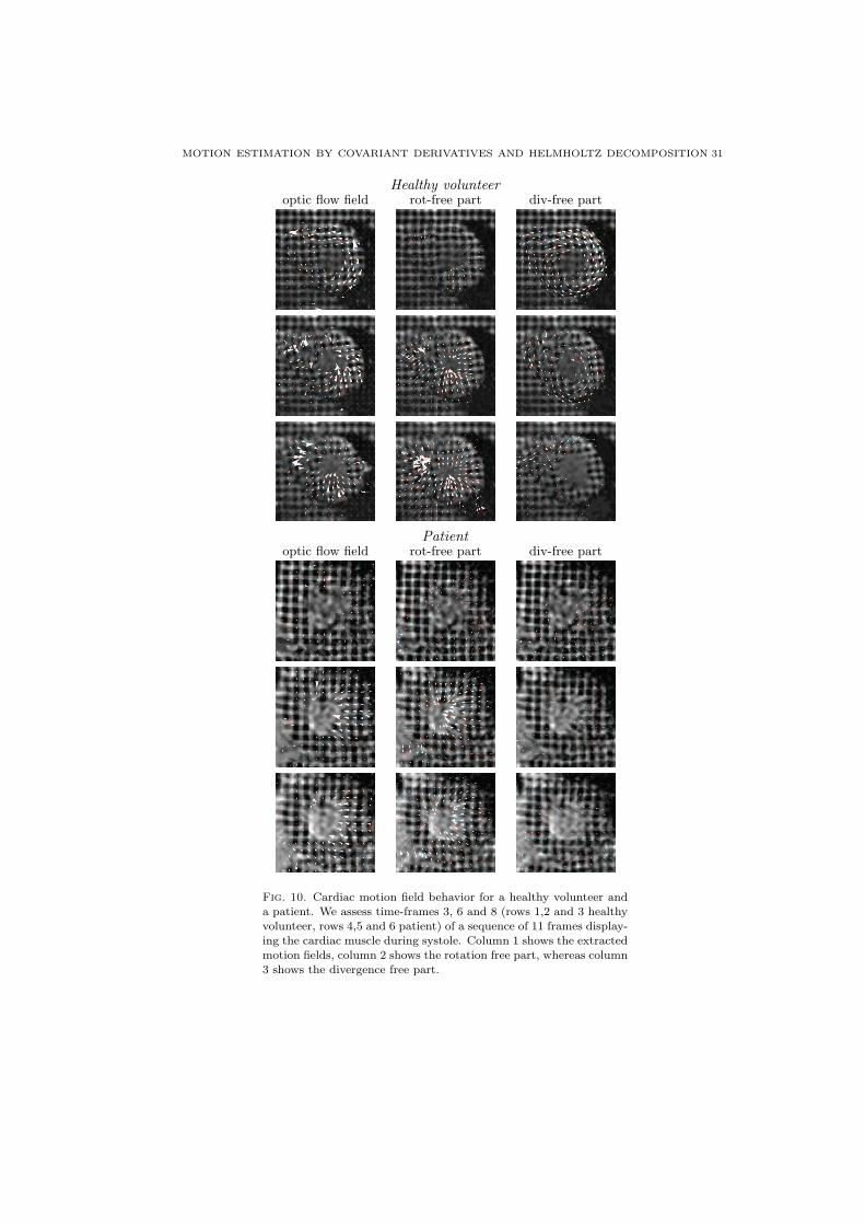
MOTION ESTIMATION BY COVARIANT DERIVATIVES AND HELMHOLTZ DECOMPOSITION 31
Healthy volunteeroptic flow field rot-free part div-free part
Patientoptic flow field rot-free part div-free part
Fig. 10. Cardiac motion field behavior for a healthy volunteer anda patient. We assess time-frames 3, 6 and 8 (rows 1,2 and 3 healthyvolunteer, rows 4,5 and 6 patient) of a sequence of 11 frames display-ing the cardiac muscle during systole. Column 1 shows the extractedmotion fields, column 2 shows the rotation free part, whereas column3 shows the divergence free part.

32 REMCO DUITS, BART JANSSEN, ALESSANDRO BECCIU, AND HANS VAN ASSEN
15. Experiments. In this section we will provide a single example of cardiac motionestimation of one healthy volunteer and of a patient whose heart is infarcted at severalareas. Acquisition of heart images has been performed during the systolic phase (i.e. thephase of the heartbeat in which the heart muscle contracts to pump blood to the restof the body); we assess 11 frames with a size of 86 × 86 pixels and pixel size of 1.37mm2 with a slice-thickness of 8 mm and a temporal resolution of 0.02 seconds. In Figure10 we respectively show the sampled motion field (column 1), rotation free (column 2)and divergence free (column 3) parts of frames 3,6 and 8 for the healthy heart case(row 1,2,3) and the diseased case (rows 4,5,6) respectively. By means of the Helmholtzdecomposition we observe that the healthy cardiac muscle starts to systole with intenserotation (row 1, column 3) and little contraction (row 1, column 2). At mid-systole, thecontribution of rotation free parts becomes qualitatively similar to the contribution ofthe divergence free part, that is, vectors inside the cardiac walls are of similar length(row 2, columns 2 and 3). At the end of the systolic phase, contraction becomes morerelevant (row 3, column 2), whereas rotation is nearly absent (row 3, column 3). Inthe investigated diseased heart case, the heart exerts modest rotation through the wholesequence (rows 4,5,6 and column 3), leaving contraction as the dominant contribution tothe heart cycle (rows 4,5,6 and column 2).
For further detailed experiments of our algorithm on analytic ground truth phantoms,comparisons between different related optic flow methods and comparisons between dif-ferent parameter settings, we refer to our technical report [12] and [4]. These experimentsshow the practical benefits of both including multi-scale Helmholtz decompositions andcovariant derivatives in our optical flow estimations.
In [4, Ch.5] our method is also compared to other established optic flow methods[44, 29, 59] by applying it to an artificial phantom dataset (cf. [4, Ch.5.2] also used in[58]) for which the ground truth is known. Our method performed best in terms ofaverage angular errors [3] and magnitude errors, cf. [4, Table 5.1,Table 5.2].
Acknowledgements. We gratefully thank Dr. J.J.M. Westenberg of Leiden Univer-sity Medical Center for providing us the cardiac MR-dataset that we used as input inSection 15 of this article.
Appendix A. Derivation of the Green’s function of the 1D covariant Lapla-cian and related (in)equalities . In this section we derive the Green’s function andprove equalities (8.3), (8.4), (8.5) and (8.6).Let h ∈ C2([0, 1]), h > 0 and consider the following PDE system on [0, 1]
(Dh)∗Dhf = δy and f ∈ H10([0, 1]), i.e. f ∈ H1([0, 1]) and f(0) = f(1) = 0.
By the Lax-Milgram theorem, this problem has a unique solution; point evaluation ψ 7→δy(ψ) = ψ(y) is a continuous linear functional on H1
0([0, 1]) and the left hand side is abounded, coercive sesquilinear form on H1
0([0, 1]). Now we set φ := Dhf ∈ L2([0, 1]) then(Dh)∗φ = 0 implies that −φ′ − h′
h φ = 0, i.e. φh′ + φ′ h = 0 ⇔ h(x)φ(x) = c1 for all

MOTION ESTIMATION BY COVARIANT DERIVATIVES AND HELMHOLTZ DECOMPOSITION 33
x ∈ [0, 1] and some c1 ∈ R. The substitution φ(x) = f ′(x)− h′(x)h(x) f(x) yields
f ′(x)h(x)− h′(x)f(x) = c1 .
This first order ODE has as homogeneous solution f = c2h and by the variation ofconstants formula we find the following standard solutions of the ODE (Dh)∗Dhf = 0:
f(x) = c2h(x) + c1 h(x) Qh(x), with Qh(x) :=∫ x
0
h(v)−2dv .
Now we find solutions f0 and f1 with f0(0) = 0, f0(1) = 1, f1(0) = 1 and f1(1) = 0:
f0(x) =h(x)Qh(x)h(1)Qh(1)
and f1(x) =h(x)(Qh(1)−Qh(x))
h(0)Qh(1).
The (constant) Wronskian of these solutions equals W = f ′0(0)f1(0) − f0(0)f ′1(0) =1
Qh(1)h(1)h(0) . Now the kernel operator Kh given by (8.3) and (8.2) can be written as
k(x, y) = 1W
f0(x)f1(y) x ≤ y,
f0(y)f1(x) x > y,⇒
(Khf)(x) = 1W
(f1(x)
x∫0
f0(y)f(y) dy + f0(x)1∫x
f1(y)f(y) dy
).
Operator Kh is the right inverse of the operator (Dh)∗Dh, where we note that Khf ∈H2
0([0, 1]) and (Dh)∗DhKhf = f , since
Kf ′′(x) =1W
(f ′′1 (x)
∫ x
0
f0(y)f(y)dy − f ′′0 (x)∫ 1
x
f1(y)f(y)dy −Wf(x))
,
so indeed −(Kf)′′ + h′′h Khf = f . Regarding (8.6) we note that kh(x, y) = kh(y, x) and
‖Kh‖2 ≤ |||Kh|||2 = traceK∗hKh = ‖kh‖2L2([0,1]×[0,1])
≤ 2(Qh(1))2
1∫0
y∫0
h2(x)h2(y)Q2h(x)(Qh(1)−Qh(y))2dxdy
= 2(Qh(1))2
∫ 1
0h2(y)(Qh(1)−Qh(y))2
(∫ y
0h2(x)Q2(x)dx
)dy
≤ 2(Qh(1))2‖h‖4L2([0,1]) = 2(
1∫0
h−2(y)dy
)2 (1∫0
h2(y)dy
)2
,
where we used that 0 ≤ Q(x) ≤ Q(1).A.1. Proof of Lemma 8.3. This follows from the fact that both f0 and f1 and their
Wronskian are positive (due to 0 ≤ Q(x) ≤ Q(1)), so for example suppose x ≤ y then∂2
∂x2 kh(x, y) = W−1f ′′0 (x)f1(y) = h′′(x)h(x) (W−1f0(x)f1(x)) ¤
References
[1] G.B. Arfken and H.J. Weber, Mathematical methods for physicists, Academic Press, San Diego,1995.
[2] L. Axel and L. Dougherty, MR imaging of motion with spatial modulation of magnetization, Radi-ology 171 (1989), no. 3, 841–845.
[3] J.L. Barron, D.J. Fleet, and S. Beauchemin, Performance of optical flow techniques, IJCV 12(1994), no. 1, 43–77.
[4] A. Becciu, Feature based estimation of myocardial motion from tagged MR images, Ph.D. thesis,Eindhoven University of Technology, Dep. of Biomedical Engineering, 2010.

34 REMCO DUITS, BART JANSSEN, ALESSANDRO BECCIU, AND HANS VAN ASSEN
[5] A. Becciu, B.J. Janssen, H.C. van Assen, L.M.J. Florack, V. Roode, and B.M. ter Haar Romeny,Extraction of cardiac motion using scale-space features points and gauged reconstruction, CAIP ’09:Proceedings of the 13th International Conference on Computer Analysis of Images and Patterns(Berlin, Heidelberg), Springer-Verlag, 2009, pp. 598–605.
[6] A. Bruhn, J. Weickert, T. Kohlber, and C. Schnoerr, A multigrid platform for real-time motioncomputation with discontinuity-preserving variational methods, IJCV 70 (2006), no. 3, 257–277.
[7] T. Corpetti, E. Memin, and P. Perez, Dense estimation of fluid flows, IEEE PAMI 24 (2002), no. 3,365–380.
[8] A. Cuzol, P. Hellier, and E. Memin, A low dimensional fluid motion estimator, International Journalof Computer Vision 75 (2007), no. 3, 329–349.
[9] J. Damon, Local Morse theory for solutions to the heat equation and Gaussian blurring, Journal ofDifferential Equations 115 (1995), no. 2, 368–401.
[10] T. Delhaas, J. Kotte, and et al. van der Toorn, A., Increase in Left Ventricular Torsion-to-Shortening Ratio in Children With Valvular Aorta Stenosis., Magnetic Resonance in Medicine51 (2004), 135–139.
[11] R. Duits, Perceptual organization in image analysis, Ph.D. thesis, Eindhoven University of Tech-nology, Department of Biomedical Engineering, The Netherlands, 2005.
[12] R. Duits, A. Becciu, B.J. Janssen, H.C. van Assen, L.M.J. Florack, and B.M. ter Haar Romeny, Car-diac motion estimation using covariant derivatives and helmholtz decomposition, CASA-report 31,Eindhoven University of Technology, Department of Mathematics and Computer Science, 2010,http://www.win.tue.nl/casa/research/casareports/2010.html.
[13] R. Duits, H. Fuehr, B.J. Janssen, and L.C.M. Bruurmijn, Left invariant reassignment and diffusionon gabor transforms, (2011), Submitted.
[14] R. Duits, B.J. Janssen, F.M.W. Kanters, and L.M.J. Florack, Linear image reconstruction from asparse set of alpha scale space features by means of inner products of Sobolev type, Lecture Notesin Computer Science, Springer-Verlag 3753 (2005), 96–111.
[15] L.C. Evans, Partial differential equations, Graduate Studies in Mathematics Vol.19 AMS, Provi-dence, 1998.
[16] L.M.J. Florack, Image structure, Computational Imaging and Vision, Kluwer Academic Publishers,Dordrecht, The Netherlands, 1997.
[17] , Scale space representations locally adapted to the geometry of base and target manifold,Mathematical Methods for Signal and Image Analysis and Representation (L.M.J. Florack, R. Duits,M.-C. Jongbloed, G. van Lieshout, and L. Davies, eds.), Springer-Verlag, 2011, pp. 175–189.
[18] L.M.J. Florack and A. Kuijper, The topological structure of scale-space images, Journal of Mathe-matical Imaging and Vision 12 (2000), no. 1, 65–79.
[19] L.M.J. Florack, W. Niessen, and M. Nielsen, The intrinsic structure of optic flow incorporatingmeasurements of duality, IJCV 27 (1998), no. 3, 263–286.
[20] L.M.J. Florack and H.C. van Assen, A New Methodology for Multiscale Myocardial Deformationand Strain Analysis Based on Tagging MRI, International Journal of Biomedical Imaging (2010),1–8, Published online http://downloads.hindawi.com/journals/ijbi/2010/341242.pdf.
[21] P.E. Forssen, Low and medium level vision using channel representations, Ph.D. thesis, LinkopingUniversity, Dept. EE, Linkoping, Sweden, March 2004.
[22] D. Gabor, Theory of communication, J. IEE 93 (1946), no. 26, 429–457.[23] T. Georgiev, Relighting, retinex theory, and perceived gradients, Proceedings of Mirage 2005, INRIA
Rocquencourt, 2005.[24] S. Gerschgorin, Ueber die abgrenzung der eigenwerte einer matrix, Izv. Akad. Nauk. USSR Otd.
Fiz.-Mat. Nauk. 7 (1931), 550–559.[25] C.W. Groetsch, Elements of applicable functional analysis, Marcel Dekker Inc., New York, Basel,
1980.[26] S. Gupta, E.N. Gupta, and J.L. Prince, Stochastic models for div-curl optical flow methods, IEEE
Signal Processing Letters 3 (1996), 32–35.[27] P.C. Hansen, J.G. Nagy, and D.P. O’Leary, Deblurring images: Matrices, spectra, and filtering, 1
ed., SIAM, 2006.[28] C.O. Horgan and S. Nemat-Nasser, Bounds on eigenvalues of Sturm-Liouville problems with dis-
continuous coefficients, Journal of Applied Mathematics and Physics 30 (1979), 77–86.[29] B.K.P. Horn and B.G. Shunck, Determining optical flow, AI 17 (1981), 185–203.

MOTION ESTIMATION BY COVARIANT DERIVATIVES AND HELMHOLTZ DECOMPOSITION 35
[30] T. Iijima, Basic theory on normalization of a pattern (in case of typical one-dimensional pattern),Bulletin of Electrical Laboratory 26 (1962), 368–388.
[31] B.J. Janssen, Representation and manipulation of images based on linear functionals, Ph.D. thesis,Eindhoven University of Technology, Eindhoven, The Netherlands, 2009.
[32] B.J. Janssen and R. Duits, Linear image reconstruction by Sobolev norms on the bounded domain.,International Journal of Computer Vision. 84 (2009), no. 2, 205–219.
[33] B.J. Janssen, R. Duits, and L.M.J. Florack, Coarse-to-fine image reconstruction based on weighteddifferential features and background gauge fields, LNCS 5567 (2009), 377–388.
[34] B.J. Janssen, L.M.J. Florack, R. Duits, and B.M. ter Haar Romeny, Optic flow from multi-scaledynamic anchor point attributes, Image Analysis and Recognition, Third International Conference,ICIAR 2006 (Berlin) (A. Campilho and M. Kamel, eds.), LNCS, vol. 4141, Springer Verlag, Sep-tember 2006, pp. 767–779.
[35] B.J. Janssen, F.M.W. Kanters, R. Duits, L.M.J. Florack, and B.M. ter Haar Romeny, A linearimage reconstruction framework based on Sobolev type inner products., International Journal ofComputer Vision 70 (2006), no. 3, 231–240.
[36] F.M.W. Kanters, T. Denton, A. Shokoufandeh, L.M.J. Florack, and B.M. ter Haar Romeny, Com-bining different types of scale space interest points using canonical sets, Scale Space and VariationalMethods (Berlin) (F. Sgallari, A. Murli, and N. Paragios, eds.), LNCS, vol. 4485, Springer Verlag,2007, pp. 374–385.
[37] F.M.W. Kanters, L.M.J. Florack, R. Duits, B. Platel, and B.M. ter Haar Romeny, Scalespaceviz:α-scale spaces in practice, Pattern Recognition and Image Analysis 17 (2007), no. 1.
[38] F.M.W. Kanters, B. Platel, L.M.J. Florack and B.M. ter Haar Romeny, Image reconstruction frommultiscale critical points, Scale Space Methods in Computer Vision, 4th International Conference,Scale Space 2003 (Isle of Skye, UK) (Lewis Griffin and Martin Lillholm, eds.), Springer, June 2003,pp. 464–478.
[39] J.J. Koenderink, The structure of images, Biol. Cybern. 50 (1984), 363–370.[40] T. Kohlberger, E. Memin, and P. Perez, Variational dense motion estimation using the Helmholtz
decomposition, LNCS Proc. Scale Space Conference (Griffin. L.D. and M. Lillholm, eds.), vol. 2695,Springer-Verlag, 2003, pp. 432–448.
[41] M. Lillholm, M. Nielsen, and L.D. Griffin, Feature-based image analysis, IJCV 52 (2003), no. 2/3,73–95.
[42] T. Lindeberg, Scale-space for discrete signals, PAMI 12 (1990), no. 3, 234–245.[43] , Scale-space theory in computer vision, The Kluwer International Series in Engineering and
Computer Science, Kluwer Academic Publishers, 1994.[44] B. Lucas and T. Kanade, An iterative image registration technique with application to stereo vision,
DARPA, Image Process, vol. 21, 1981, pp. 85–117.[45] P.D. Milgram and A.N. Lax, Parabolic equations, Contributions to the theory of partial differential
equations, Annals of Math. Studies 30 (1954), 167–190.[46] I. Mirsky, J.M. Pfeffer, and et al. Pfeffer M.A., The contractile state as the major determinant
in the evolution of left ventricular dysfunction in the spontaneously hypertensive rat. CirculationResearch, 53 (1983), 767–778.
[47] M. Nielsen and M. Lillholm, What features tell about images?, LNCS 2106 (2001), 39–50.[48] T. Nir, A.M. Bruckstein, and R. Kimmel, Over-Parameterized variational optical flow, International
Journal of Computer Vision 76 (2008), no. 2, 205–216.[49] N.F. Osman, W.S. McVeigh, and J.L. Prince, Cardiac motion tracking using cine harmonic phase
(harp) magnetic resonance imaging, Magnetic Resonance in Medicine 42 (1999), no. 6, 1048–1060.[50] W. Rudin, Functional analysis, McGraw-Hill, New York, 1973.[51] Y. Saad, Iterative methods for sparse linear systems (2nd edition), SIAM, 2004.[52] Sheehan, F. and Stewart, D. and Dodge, H. and Mitten, S. and Bolson E. and Brown, G., Variability
in the measurement of regional left ventricular wall motion, Circulation 68 (1983), 550–559.[53] J. Staal, S. Kalitzin, B.M. ter Haar Romeny, and M. Viergever, Detection of critical structures in
scale space, LNCS, vol. 1682, 1999, pp. 105–116.[54] B.M. ter Haar Romeny, Front-end vision and multi- scale image analysis: Multiscale computer
vision theory and applications, written in mathematica, Computational Imaging and Vision, KluwerAcademic Publishers, Dordrecht, The Netherlands, 2003.
[55] J.P. Thirion, Image matching as a diffusion process: an analogy with Maxwells demons, MedicalImage Analysis 2 (1998), no. 3, 243–260.

36 REMCO DUITS, BART JANSSEN, ALESSANDRO BECCIU, AND HANS VAN ASSEN
[56] Y. Tong, S. Lombeyda, A.N. Hivani, and M. Desbrun, Discrete multiscale vector field decomposition,ACM Transactions on Graphics (TOG) 22 (2003), 445–452.
[57] M. Unser, Splines: A perfect fit for signal and image processing, IEEE Signal Processing Magazine16 (1999), no. 6, 22–38.
[58] H.C. van Assen, L.M.J. Florack, F.J.J. Simonis, and J.J.M. Westenberg, Cardiac strain and rotationanalysis using multi-scale optical flow, MICCAI workshop on Computational Biomechanics forMedicine 5, Springer-Verlag, 2011, pp. 91–103.
[59] H.C. van Assen, L.M.J. Florack, A. Suinesiaputra, J.J.M. Westenberg, and B.M. ter Haar Romeny,Purely evidence based multiscale cardiac tracking using optic flow, Proc. MICCAI 2007 workshop onComputational Biomechanics for Medicine II (K. Miller, K. D. Paulsen, A. A. Young, and P. M. F.Nielsen, eds.), 2007, pp. 84–93.
[60] H. von Helmholtz, Ueber integrale der hydrodynamischen gleichungen, welche den wirbelbewegungenentsprechen, Crelles J. 55 (1858), no. 25.
[61] J. Weickert, S. Ishikawa, and A. Imiya, On the history of Gaussian scale-space axiomatics, GaussianScale-Space Theory, Computational Imaging and Vision Series, Kluwer Academic Publisher, 1997,pp. 45–59.
[62] E.A. Zerhouni, D.M. Parish, W.J. Rogers, A. Yang, and E.P. Sapiro, Human heart: Tagging withMR imaging a method for noninvasive assessment of myocardial motion, Radiology 169 (1988),no. 1, 59–63.
[63] H. Zimmer, A. Bruhn, J. Weickert, L. Valgaerts, A. Salgado, B. Rosenhahn, and H.-P. Seidel,Complementary optic flow, Proceedings of Energy Minimization Methods in Computer Vision andPattern Recognition (EMMCVPR), LNCS, Berlin, Springer-Verlag, vol. 5681, 2009, pp. 207–220.