a vba based computer program for nonlinear fea of large displacement 2d beam structures

www.ijraset.com Volume 3 Issue IX, September 2015 IC Value: 13.98 ISSN: 2321-9653

International Journal for Research in Applied Science & Engineering Technology (IJRASET)

©IJRASET 2015: All Rights are Reserved 1

A VBA Based Computer Program for Nonlinear FEA of Large Displacement 2D Beam Structures

Sreekanth M. Sivaraman Technip Geoproduction Sdn Bhd, Malaysia

Abstract— This article proposes a methodology for implementing a VBA based nonlinear FEA program in Microsoft Excel, for analyzing large displacement 2D beam structures. The program uses 2 noded - 6 degrees of freedom elements, and the equilibrium equations were formulated in combined Corotational - Total Lagrangian (CR-TL) system. Polynomial operation capability was built into the program, enabling computerized generation of stiffness and nodal force matrices. This makes the program easily adaptable to various element formulations. The program was also equipped with the mathematical functionality required for efficient handling of computations involving nonlinear strain measures. Accuracy and limitations of the program are demonstrated through NAFEMS benchmark tests. Keywords— Nonlinear FEA program; Large displacement beam; Corotational system; CR-TL system; Beam element benchmark test; FEA program development

I. INTRODUCTION Finite Element Analysis of large displacement beam structures has extensive utility in several branches of engineering, one prime example being offshore pipeline engineering. Many commercial software packages are available for such analyses and usually these softwares are tailor made to analyse specific situations that occur commonly during engineering operations. Though there are advantages to using such softwares, there is a major drawback that the engineers have to work with a limited set of methodologies and formulations. Often the problem at hand needs to be modified significantly to suit the features of the software package. Therefore importance of custom developed applications cannot be overstated. Many efficient frameworks and methodologies for building nonlinear FEA programs have been proposed till date. Some of them are ([1]-[4]). Most of the existing works present succinct overviews of software architecture that is suitable for large scale programs. There is a lack of literature that focuses on computational aspects of a program. This article aims to present such an approach, by discussing implementation of a FEA program in Microsoft Excel for analysing geometrically nonlinear 2 dimensional beam structures. Microsoft Excel was chosen as it is a platform easily available to practicing engineers and students. The chart and spreadsheet features of Excel provide means of interfacing with the user. Several methodologies for solving geometrically nonlinear problems have been proposed till date, and most of the methods are based on Total Lagrangian (TL), Updated Lagrangian (UL), Corotational (CR) formulations or a combination of them ([5]-[10]). While the strong suit of CR formulation is the handling of large rotations, UL and TL methods help in considering large element deformations. Therefore, a combination of these methods helps to handle large element strains as well as displacements and rotations. The accuracy in large strain analysis also depends on the displacement interpolation functions used. Exact interpolations functions for 2D and 3D beam elements have been proposed in the past ([11]-[13]), but analyses can be done with approximate functions as well. This program uses cubic Hermitian polynomials for transverse nodal displacements, and linear polynomials for axial displacements. Benchmark tests were done against geometrically exact formulations, which reveal the limitations and capabilities of the program. Section VI presents the results of the benchmark tests. A brief summary of the program is given in Fig. 1.

II. BASIC FUNCTIONALITY

A. Polynomial Operations Since nonlinear strain and stress measures were used, calculation of stiffness and nodal force matrices during analysis involved integration of several high order polynomials. In order to make the program easily adaptable to various interpolation functions, a data type was defined to hold polynomials, and functions were defined for conducting mathematical operations using polynomials and polynomial matrices. Polynomials were defined using 2 dimensional arrays (size - n x m) where ‘(n – 1)’ is the exp ected number of variables and ‘m’ is the number of terms in the polynomial. Each expected variable is assigned a row number and each term of the polynomial is assigned a column number. Member (i, j) of the array contains the degree of the (i-1)th variable of the jth




term of the polynomial. An example is shown in Fig. 2. Custom functions were defined for addition, multiplication, differentiation, integration and other required polynomial operations. Three types of polynomials were defined - Type 1 - with variables x, y, E (Young’s modulus), L (element length), 1/(1 + ν) (ν = Poisson’s ratio) . Type 2 - with variables cosθ, sinθ, L . Type 3 - with variables E, L and 1/ (1 + ν)

Fig. 1 Summary of the program

Polynomial - xy/L + 3y3E/L2 1 3 - Coefficient 1 0 - Degree of x 1 3 - Degree of y 0 1 - Degree of E -1 -2 - Degree of L

Fig. 2 Array representation of a polynomial

B. Matrix Operations Since FEA involves several matrix operations, the ‘array’ feature of VBA was extensively used. In addition to the numerical array

Read and process input

Read model definition – Nodes, elements, section profiles, material properties, load and boundary conditions, analysis step details and prepare data arrays.

Mesh the structure, and assign numbers to nodes, elements and all nodal degrees of freedom.

Plot the structure

Define general matrices

Define displacement interpolation functions, material constitutive law and co-ordinate transformation matrices

Integrate and prepare element stiffness matrices and nodal force matrices in generalized format.

Analyse the structure for each step

Identify loads and boundary conditions initiated in the current step and ones that are propagated from the previous step

Attempt to find equilibrium configuration at the end of the step.

Plot and print results

Print output data Plot the required configurations




operation functions inbuilt in VBA, several other matrix operations involving block matrices were required during the program execution. Custom functions were defined for these. Details of some of these functions, along with their names (which will be referred to later in this article), are given in Table I.

C. User Interface And Input Data Handling Since User interface of the program was based on spreadsheet cells and charts. Input data entered in designated cells was read and stored in specific arrays (Refer Table II). The required input data consisted of details of nodes, elements, section profiles, element properties, load and boundary conditions, and analysis step details.

1) Loads and Boundary Conditions: The load types considered in the program were joint loads (Forces/moments on user defined nodes), uniform line forces and uniform body forces. Applicable boundary conditions consist of displacements/rotations at user defined nodes. Conducting multi-step analysis would require the user to define the analysis steps in which a particular load or boundary condition is to be applied. In this program, load or boundary condition definition included input for the starting and ending steps (Refer Table II).

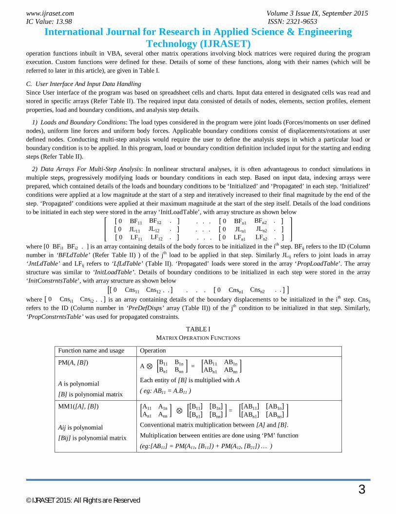
2) Data Arrays For Multi-Step Analysis: In nonlinear structural analyses, it is often advantageous to conduct simulations in multiple steps, progressively modifying loads or boundary conditions in each step. Based on input data, indexing arrays were prepared, which contained details of the loads and boundary conditions to be ‘Initialized’ and ‘Propagated’ in each step. ‘Initialized’ conditions were applied at a low magnitude at the start of a step and iteratively increased to their final magnitude by the end of the step. ‘Propagated’ conditions were applied at their maximum magnitude at the start of the step itself. Details of the load conditions to be initiated in each step were stored in the array ‘InitLoadTable’, with array structure as shown below

[ 0 BF11 BF12 . ] [ 0 JL11 JL12 . ]

[ 0 LF11 LF12 . ]

. . .[ 0 BFn1 BFn2 . ] . . .[ 0 JLn1 JLn2 . ] . . .[ 0 LFn1 LFn2 . ]

where [0 BFi1 BFi2 . ] is an array containing details of the body forces to be initialized in the ith step. BFij refers to the ID (Column number in ‘BFLdTable’ (Refer Table II) ) of the jth load to be applied in that step. Similarly JLij refers to joint loads in array ‘JntLdTable’ and LFij refers to ‘LfLdTable’ (Table II). ‘Propagated’ loads were stored in the array ‘PropLoadTable’. The array structure was similar to ‘InitLoadTable’. Details of boundary conditions to be initialized in each step were stored in the array ‘InitConstrntsTable’, with array structure as shown below

[ 0 Cns11 Cns12 . . ] . . . [ 0 Cnsn1 Cnsn2 . . ] where [ 0 Cnsi1 Cnsi2 . . ] is an array containing details of the boundary displacements to be initialized in the ith step. Cnsij refers to the ID (Column number in ‘PreDefDisps’ array (Table II)) of the jth condition to be initialized in that step. Similarly, ‘PropConstrntsTable’ was used for propagated constraints.

TABLE I MATRIX OPERATION FUNCTIONS

Function name and usage Operation

PM(A, [B]) A is polynomial [B] is polynomial matrix

A ⊗ B11 B1nBn1 Bnn

= AB11 AB1nABn1 ABnn

Each entity of [B] is multiplied with A ( eg: AB11 = A.B11 )

MM1([A], [B]) Aij is polynomial [Bij] is polynomial matrix

A11 A1nAn1 Ann

⊗[B11] [B1n][Bn1] [Bnn] =

[AB11] [AB1n][ABn1] [ABnn]

Conventional matrix multiplication between [A] and [B]. Multiplication between entities are done using ‘PM’ function (eg:[AB11] = PM(A11, [B11]) + PM(A12, [B21]) … )




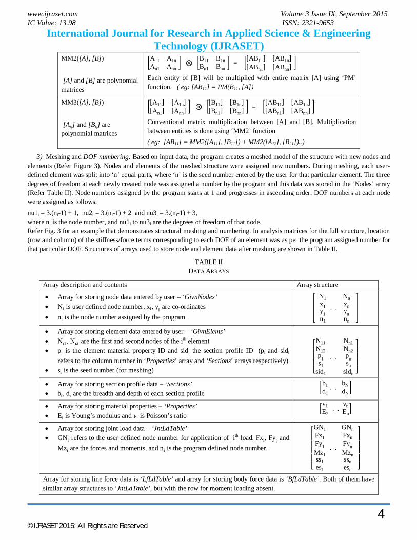
MM2([A], [B]) [A] and [B] are polynomial matrices

A11 A1nAn1 Ann

⊗ B11 B1nBn1 Bnn

= [AB11] [AB1n][ABn1] [ABnn]

Each entity of [B] will be multiplied with entire matrix [A] using ‘PM’ function. ( eg: [AB11] = PM(B11, [A])

MM3([A], [B]) [Aij] and [Bij] are polynomial matrices

[A11] [A1n][An1] [Ann] ⊗

[B11] [B1n][Bn1] [Bnn] =

[AB11] [AB1n][ABn1] [ABnn]

Conventional matrix multiplication between [A] and [B]. Multiplication between entities is done using ‘MM2’ function ( eg: [AB11] = MM2([A11], [B11]) + MM2([A12], [B21])..)

3) Meshing and DOF numbering: Based on input data, the program creates a meshed model of the structure with new nodes and elements (Refer Figure 3). Nodes and elements of the meshed structure were assigned new numbers. During meshing, each user-defined element was split into ‘n’ equal parts, where ‘n’ is the seed number entered by the user for that particular element. The three degrees of freedom at each newly created node was assigned a number by the program and this data was stored in the ‘Nodes’ array (Refer Table II). Node numbers assigned by the program starts at 1 and progresses in ascending order. DOF numbers at each node were assigned as follows. nu1i = 3.(ni-1) + 1, nu2i = 3.(ni-1) + 2 and nu3i = 3.(ni-1) + 3, where ni is the node number, and nu1i to nu3i are the degrees of freedom of that node. Refer Fig. 3 for an example that demonstrates structural meshing and numbering. In analysis matrices for the full structure, location (row and column) of the stiffness/force terms corresponding to each DOF of an element was as per the program assigned number for that particular DOF. Structures of arrays used to store node and element data after meshing are shown in Table II.

TABLE II DATA ARRAYS

Array description and contents Array structure

Array for storing node data entered by user – ‘GivnNodes’ Ni is user defined node number, xi, yi are co-ordinates ni is the node number assigned by the program

N1x1y1n1

. .

Nnxnynnn

Array for storing element data entered by user – ‘GivnElems’ Ni1, Ni2 are the first and second nodes of the ith element pi is the element material property ID and sidi the section profile ID (pi and sidi

refers to the column number in ‘Properties’ array and ‘Sections’ arrays respectively) si is the seed number (for meshing)

⎣⎢⎢⎢⎡N11N12p1s1

sid1

. .

Nn1Nn2pnsn

sidn

⎦⎥⎥⎥⎤

Array for storing section profile data – ‘Sections’ bi, di are the breadth and depth of each section profile

b1d1

. . bNdN

Array for storing material properties – ‘Properties’ Ei is Young’s modulus and 휈i is Poisson’s ratio

ν1E2

. . νnEn

Array for storing joint load data – ‘JntLdTable’ GNi refers to the user defined node number for application of ith load. Fxi, Fyi and

Mzi are the forces and moments, and ni is the program defined node number.

⎣⎢⎢⎢⎢⎡GN1Fx1Fy1Mz1ss1es1

. .

GNnFxnFynMznssnesn

⎦⎥⎥⎥⎥⎤

Array for storing line force data is ‘LfLdTable’ and array for storing body force data is ‘BfLdTable’. Both of them have similar array structures to ‘JntLdTable’, but with the row for moment loading absent.




Array for storing boundary displacements – ‘PreDefDisps’ GNi refers to the user defined node number for application of ith displacement. Δi is

the displacement ssi and esi are the starting and ending steps ⎣

⎢⎢⎢⎡

GN1DOF1

Δ1ss1es1

. .

GNnDOFn

Δnssnesn

⎦⎥⎥⎥⎤

Array for storing node details of meshed structure - ‘Nodes’ xi, yi are co-ordinates of ith node, nu1i, nu2i and nu3i are the numbering of the

degrees of freedom at each node.

⎣⎢⎢⎢⎢⎡

n1x1y1

nu11nu21nu31

. .

nnxnyn

nu1nnu2nnu3n

⎦⎥⎥⎥⎥⎤

Array for storing element details of meshed structure is ‘Elements’, which has similar structure as ‘GivnElems’ array.

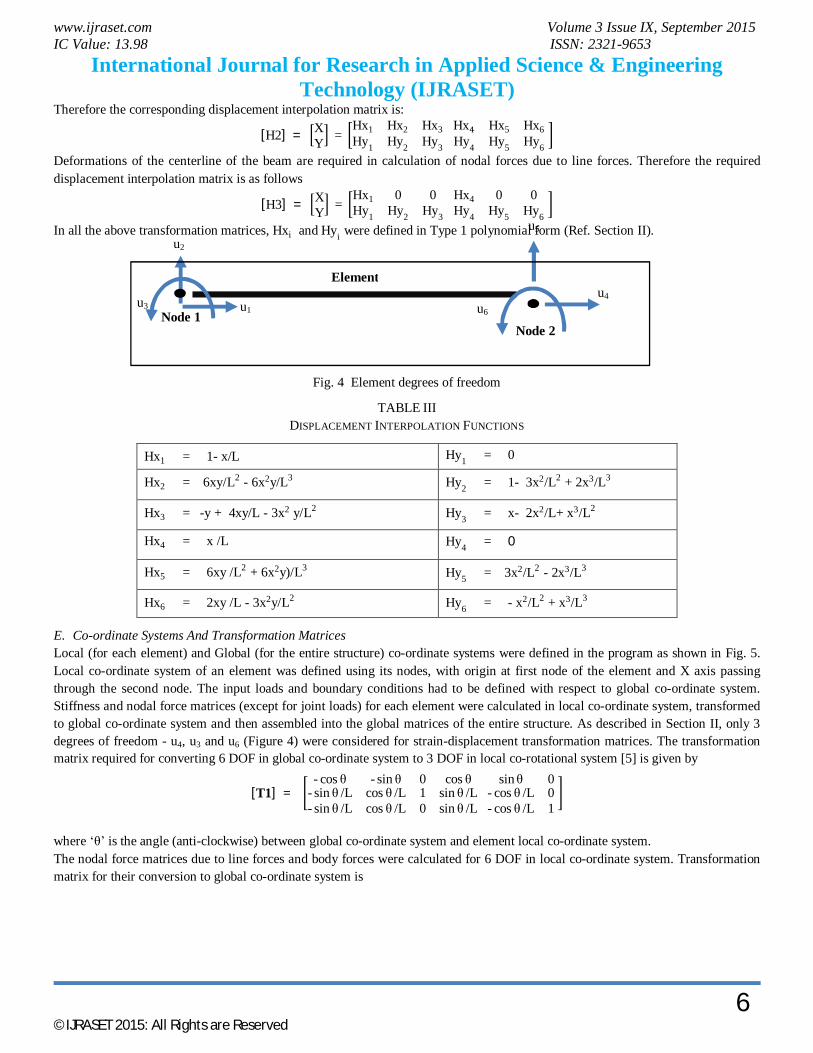
D. Displacement Interpolation Functions Displacement fields within the element were defined by Hermitian polynomials. Shear deformations were not considered. The 6 nodal degrees of freedom were numbered as shown in Figure 4. u3 and u6 are the slopes of rotational displacements at the element nodes. Displacement interpolation functions corresponding to each degree of freedom ‘i', designated as Hxi and Hyi (for X and Y directions respectively) are shown in Table III. For definition of the interpolation functions, the origin of co-ordinates was considered to be node 1, with X axis located along element axis. Since strains and stresses were calculated in co-rotational system [5], only three degrees of freedom are relevant for strain-displacement transformation matrix – u4, u3 and u6. Displacement interpolation matrix used for strain calculations is shown below.

[H1] = XY =

Hx4 Hx3 Hx6 Hy4 Hy3 Hy6

User defined structure

Program defined structure (after meshing)

Numbering of degrees of freedom

Fig. 3 Meshing and DOF numbering

The displacement fields due to all 6 DOF are relevant for the calculation of nodal force components due to applied body forces.

6 9 18 15

3

8

12

5 2

16

14

13

11

10 7

1

4

17

N2 N3

1 2

3 5 4

1 3 4

6 2 Elements Nodes

1

2 5

N1

Nodes Elements




Therefore the corresponding displacement interpolation matrix is:

[H2] = XY =

Hx1 Hx2 Hx3Hy1 Hy2 Hy3

Hx Hx5 Hx6Hy4 Hy5 Hy6

Deformations of the centerline of the beam are required in calculation of nodal forces due to line forces. Therefore the required displacement interpolation matrix is as follows

[H3] = XY =

Hx1 0 0Hy1 Hy2 Hy3

Hx4 0 0Hy4 Hy5 Hy6

In all the above transformation matrices, Hxi and Hyi were defined in Type 1 polynomial form (Ref. Section II).

Fig. 4 Element degrees of freedom

TABLE III DISPLACEMENT INTERPOLATION FUNCTIONS

Hx1 = 1- x/L Hy1 = 0

Hx2 = 6xy/L2 - 6x2y/L3 Hy2 = 1- 3x2/L2 + 2x3/L3

Hx3 = -y + 4xy/L - 3x2 y/L2 Hy3 = x- 2x2/L+ x3/L2

Hx4 = x /L Hy4 = 0

Hx5 = 6xy /L2 + 6x2y)/L3 Hy5 = 3x2/L2 - 2x3/L3

Hx6 = 2xy /L - 3x2y/L2 Hy6 = - x2/L2 + x3/L3

E. Co-ordinate Systems And Transformation Matrices Local (for each element) and Global (for the entire structure) co-ordinate systems were defined in the program as shown in Fig. 5. Local co-ordinate system of an element was defined using its nodes, with origin at first node of the element and X axis passing through the second node. The input loads and boundary conditions had to be defined with respect to global co-ordinate system. Stiffness and nodal force matrices (except for joint loads) for each element were calculated in local co-ordinate system, transformed to global co-ordinate system and then assembled into the global matrices of the entire structure. As described in Section II, only 3 degrees of freedom - u4, u3 and u6 (Figure 4) were considered for strain-displacement transformation matrices. The transformation matrix required for converting 6 DOF in global co-ordinate system to 3 DOF in local co-rotational system [5] is given by

[T1] = - cos θ - sin θ

- sin θ /L- sin θ /L

cos θ /Lcos θ /L

0 cos θ10

sin θ /Lsin θ /L

sin θ 0

- cos θ /L- cos θ /L

01

where ‘θ’ is the angle (anti-clockwise) between global co-ordinate system and element local co-ordinate system. The nodal force matrices due to line forces and body forces were calculated for 6 DOF in local co-ordinate system. Transformation matrix for their conversion to global co-ordinate system is

u1

u2

u3 u4

u5

u6

Element

Node 1 Node 2




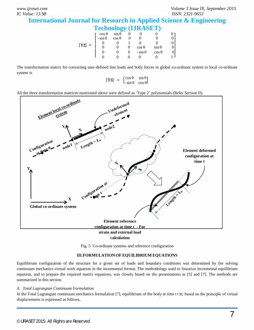
[T2] =

⎣⎢⎢⎢⎢⎡ cos θ sin θ 0 0 0 0- sin θ cos θ 0 0 0 1

0 0 00 0 00 0 0

0 0 0 0 0 0cos θ sin θ 0- sin θ cos θ 0 0 0 1 ⎦

⎥⎥⎥⎥⎤

The transformation matrix for converting user-defined line loads and body forces in global co-ordinate system to local co-ordinate system is

[T3] = cos θ sin θ- sin θ cos θ

All the three transformation matrices mentioned above were defined as ‘Type 2’ polynomials (Refer Section II).

Fig. 5 Co-ordinate systems and reference configuration

III. FORMULATION OF EQUILIBRIUM EQUATIONS

Equilibrium configuration of the structure for a given set of loads and boundary conditions was determined by the solving continuum mechanics virtual work equation in the incremental format. The methodology used to linearize incremental equilibrium equation, and to prepare the required matrix equations, was closely based on the presentations in [5] and [7]. The methods are summarized in this section.

A. Total Lagrangian Continuum Formulation In the Total Lagrangian continuum mechanics formulation [7], equilibrium of the body at time t+∆t, based on the principle of virtual displacements is expressed as follows,

X

Y

Global co-ordinate system

Element deformed configuration at

time t

Element reference configuration at time t - For

strain and external load calculation




dvδS ijtt

ijV

tt 000

0

= t+∆tR (1)

where t+∆tR is the total external virtual work due to uniform line forces with components ktt m

0 , body forces with components

ktt b

0 and nodal loads jk ,

Rtt = dLδum kkL

tt 00

0 + dvδub kk

V

tt 00

0 + kk δuj .Σ (2)

In eqn(2) kδu is the virtual variation in displacement components at time t+∆t. In eqn(1), ijttδ

0 is the virtual variation in the

Cartesian components of Green-Lagrangian (GL) strain tensor (in the configuration at time t+∆t referred to the configuration at time

0), and ijtt S

0 are the Cartesian components of the 2nd Piola-Kirchoff (PK2) stress tensor in the configuration t+∆t and measured in

the configuration at time 0.

ijtt 0 = ).(

21

,0,0,0,0 jktt

iktt

ijtt

jitt uuuu (3)

ijtt S

0 = rstt

ijrstt C

00 (4)

where itt u

0 are displacements at time t+∆t, measured in configuration at time 0, and ijrstt C

0 are the tensor components of the

constitutive relationship at time t+∆t.

B. Linearized Incremental TL Formulation As shown by Bathe and Bolorouchi [7], eqn(1) can be written in linearized incremental format as follows:

dveδeC ijrsV

ijrs0

0000 + dvδS ijij

V

t 000

0

= t+∆tR - dveδS ijijV

t 000

0 (5)

Where the strain increment ij0 , has been decomposed into

Linear part, ije0 = )..(21

,0,0,0,0,0,0 ikjkt

jkikt

ijji uuuuuu (6)

And nonlinear part, ij0 = ).(21

,0,0 jkik uu (7)

Since Total Lagrangian formulation is combined with Corotational formulation here, strain tensors at time t+∆t were calculated w.r.t. the reference configuration at time t (Figure 5). Reference configuration at time t = Undeformed element oriented along X axis of the local co-ordinate system at time t. The subscript ‘0’ in equations in this section stands for the aforementioned reference configuration.

For calculations done in the program, linear incremental strain ( ije0 ) was further divided as follows

ije0 = 10 ije + 2

0 ije (8)

, where 10 ije = )(

21

,0,0 ijji uu (9)

20 ije = )..(

21

,0,0,0,0 ikjkt

jkikt uuuu (10)

20 ije incorporates the effect of existing strains at time t, on the incremental strains.

And ijt S0 was decomposed into linear and nonlinear parts as

ijt S0 =

ijte

ijt SS 00 (11)

, where eij

t S0 = rst

ijrst eC 00 (Linear part) (12)




ij

t S0 = rst

ijrstC 00 (Nonlinear part) (13)

, where ijt e0 = )(

21

,0,0 ijt

jit uu (14)

ijt0 = ).(

21

,0,0 jkt

ikt uu (15)

Based on eqns (8) to (15), eqn(5) was decomposed as eqn(16).

dveδeC ijrsV

ijrs0

01

000 + dveδeC ijrs

Vijrs

00

200

0 + dvδS ij

eij

V

t 000

0

+ dvδS ijijV

t 000

0

= Rtt - dveδS ijeij

V

t 000

0 - dveδS ijij

V

t 000

0

(16)

C. Matrix Form Of Equilibrium Equations – Total Lagrangian Formulation The force/moment equations corresponding to eqn(16) in matrix format is calculated here as eqn(17), and that corresponding to eqn(2) as eqn(18).

[0K0]. u0 + [0K1]. u0 + [0K2]. u0 + [0K3]. u0 = [R] - [0IF1] + [0IF2] (17)

[R] = [0LF]. m0t+∆t + [0BF]. b0

t+∆t + [0JL] (18) Subscript ‘0’ indicates that the matrices in (17) and (18) are calculated w.r.t. local co-ordinate system (Figure 5). u0 is the incremental nodal displacement vector in local system, which consists of u4, u3 and u6, as described in Section II. In eqn(17), [0K0], [0K1], [0K2] and [0K3] are stiffness matrices, and [0IF1], [0IF2] are nodal load vectors corresponding to elemental internal stresses. In eqn(18), m0

t+∆t and b0t+∆t are the load vectors at time t+∆t (load per unit length and load per unit volume

respectively) for line forces and body forces in local co-ordinate system. [0LF] and [0BF] are transformation matrices for converting the distributed force vectors (in local co-ordinate system) to nodal load vectors. Combining eqns(17) and (18), equilibrium equation of an element in matrix form is

[0K0123]. u0 = [0JL] + [0LF]. m0t+∆t + [0BF]. b0

t+∆t - [0IF12] (19) ,where [0K0123] = [0K0] + [0K1] + [0K2] + [0K3] (20) and [0IF12] = [0IF1] + [0IF2] (21)

Transforming eqn (19) to global co-ordinate system,

[T1]T.[K0123].[T1].[u] = [JL] + [T2]T[0LF].[T3]. mt+∆t + [T2]T[0BF].[T3]. bt+∆t - [T1]T.[0IF12] (22) ,where [u] is the incremental nodal displacement vector in global co-ordinate system, consisting of 6 DOF. mt+∆t and bt+∆t are load vectors in global co-ordinate system. [JL] is joint load vector in global co-ordinate system. Eqn(22) can be made more effective with addition of an extra stiff ness matrix, as discussed in the next section.

D. Combining Corotational Formulation With Total Lagrangian Formulation Eqn(22) basically attempts to the find the structural configuration at time t+Δt, based on the configuration and applied loads at time t+∆t. The variation of internal load w.r.t. incremental nodal displacements is linearized, but variation of the co-ordinate system transformation matrices are ignored, which can limit solvability of problems involving large rotations. In corotational formulation, variation of the transformation matrix [T1] due to incremental nodal displacements is considered. An additional tangent stiffness matrix is thus obtained, which improves consistency of linearization. Derivation of this additional stiffness matrix is shown in eqn(23) to eqn(30), based on the presentation by Crisifield [5] Starting afresh and looking at element equilibrium again, nodal load vector corresponding to element internal stresses at time t is

[IntF] = [T1]T[0IntF] (23) ,where [IntF] , [0IntF] are element internal load matrices in global and local co-ordinate system respectively. Incremental variation of eqn(23) gives

δ[IntF] = [T1]T.δ[0IntF] + δ[T1]T.[0IntF] (24)




Left hand side (LHS) of eqn(24) represents the complete stiffness matrix in global co-ordinate system, i.e. the variation in internal forces w.r.t. incremental displacements. LHS of eqn(22) is the first term of Right hand side (RHS) of eqn(24), with some approximations due to linearization. The second term of RHS of eqn(24) is the additional stiffness matrix which captures the variation in transformation matrix [T1]. As shown by Crisifield [5],

δ[T1]T. [0IntF] = N L. ([z].[z]T).[u]+ (M1+ M2)

L. ([r].[z]T+[z].[r]T).[u] (25) ,where N is the axial force in the element, M1, M2 are end moments , L is the deformed length of the element, and

[z] =

⎣⎢⎢⎢⎢⎡

sin θ-cos θ

0- sin θcos θ

0 ⎦⎥⎥⎥⎥⎤

, [r] =

⎣⎢⎢⎢⎢⎡- cos θ- sin θ

0cos θsin θ

0 ⎦⎥⎥⎥⎥⎤

where ‘θ’ is the angle (anti-clockwise) between global co-ordinate system and element local co-ordinate system. In this program, [z] and [r] were defined as matrices with ‘Type 2’ polynomials as entities (Section II). Considering the new additional stiffness matrix as [K4], the total stiffness matrix of an element in global co-ordinate system is

[K01234] = [K0123] + [K4] (27) ,where [K0123] = [T1]T.[0K0123].[T1]

and [K4] is calculated as shown in eqn(25). Thus the equilibrium equation in global co-ordinate system becomes

[K01234].[u] = [JL] + [LF]. mt+∆t + [BF]. bt+∆t - [IF12] (28) ,where [LF] = [T2]T[0LF].[T3] (29) and [BF] = [T2]T[0BF].[T3] (30)

IV. MATRIX GENERATION ALGORITHM Accurate and efficient computation of the stiffness and nodal force matrices in eqn(28) is perhaps the most important part of a nonlinear FEA program. During analysis, these matrices need to be calculated repetitively and this can cost a major portion of runtime. When material nonlinearity is not considered, it is possible to conduct all the required integration operations prior to start of iterative analysis, which reduces runtime significantly. The methodology used in this program is to generate generalized forms of the stiffness and nodal load matrices prior to start of iterative analysis and then use them repetitively without much computational cost. The terms of these general matrices were in polynomial format (‘Type3’ polynomial form – Refer Section II), and were converted to numerical format during analysis. Sections IV-A to IV-C describe the procedures used to prepare the necessary matrices.

A. Basic Matrices Some basic block matrices were prepared prior to calculation of strain-displacement transformation matrices. They are shown below. ‘Variant’ data type in VBA was used to store these block matrices.

[dUdx] = d(Hx4)

dx

d(Hx3)dx

d(Hx6)

dx

[dVdy] = d(Hy4)

dy

d(Hy3)dy

d(Hy6)

dy

[dUdy] = d(Hx4)

dy

d(Hx3)dy

d(Hx6)

dy

[dVdx] = d(Hy4)

dx

d(Hy3)dx

d(Hy6)

dx




where Hxi and Hyi are displacement interpolation functions (Section II). d(Hxi)

dx ,

d(Hyi)

dx were ‘Type 1’ polynomials calculated using

custom made functions for differentiation of ‘Type 1’ polynomials. Using the basic matrices above, the following matrices were calculated

[dUdxdUdx] = [dUdx]T.[dUdx]

[dUdydUdy] = [dUdy]T.[dUdy]

[dUdxdUdy] = [dUdx]T.[dUdy]

[dUdydUdx] = [dUdy]T.[dUdx]

[dVdxdVdx] = [dVdx]T.[dVdx]

[dVdydVdy] = [dVdy]T.[dVdy]

[dVdxdVdy] = [dVdx]T.[dVdy]

[dVdydVdx] = [dVdy]T.[dVdx]

B. Strain-Displacement And Stress-Displacement Transformation Matrices Transformation matrices for various strain and stress tensors were calculated as described here. The strain-displacement transformation matrix for ij

t e0 was defined as a block matrix. Transformation matrix for each strain component were defined

separately, and combined into a single matrix as shown below. Considering a single component of strain, xx

t e0 = xxu ,0 = [dUdx].[ u0t ] = [GLe0xx].[ u0

t ]

i.e. [GLe0xx] = [dUdx] (31) where [ u0

t ] is nodal displacement vector in corotational system at time t. Calculation of [ u0t ] is discussed in Appendix A.

Similarly,

[GLe0yy] = [dVdy] (32)

[GLe0xy] = [dUdy] + [dVdx] (33)

Combining the eqns(31) to (33), [GLe] = [GLe0xx][GLe0yy][GLe0xy]

[GLe] was defined as a block matrix to suit the computations that were to be done using it later. Strain-displacement transformation matrix for ij

t0 was also defined as a block matrix, as follows.

Considering a single strain component,

xxt0 = )(

21

,0,0,0,0 xyt

xyt

xxt

xxt uuuu

= 21 ( [dUdx].[ u0

t ].[dUdx].[ u0t ] + [dVdx].[ u0

t ].[dVdx].[ u0t ] )

= 21 ( [ u0

t ]T.[dUdx]T.[dUdx].[ u0t ] + [ u0

t ]T.[dVdx]T.[dVdx].[ u0t ] )

= 21 ([ u0

t ]T. [dUdx]T.[dUdx] + [dVdx]T.[dVdx] .[ u0t ])

= 21 ([ u0

t ]T. [dUdxdUdx] + [dVdxdVdx] .[ u0t ] )

= 21 ( [ u0

t ]T.[GLn0xx].[ u0t ] )




i.e. [GLn0xx] = 21 ( [dUdxdUdx] + [dVdxdVdx] ) (34)

Similarly,

[GLn0yy] = 21 ( [dUdydUdy] + [dVdydVdy] ) (35)

[GLn0xy] = 21 ( [dUdxdUdy] + [dVdxdVdy] ) (36)

[GLn0yx] = 21 ( [dUdydUdx] + [dVdydVdx] ) (37)

Combining eqns(34) to (36), [GLn] was defined as [GLn0xx][GLn0yy][GLn0xy]

Strain-displacement transformation matrix for 10 ije was defined as,

[B0] =

⎣⎢⎢⎢⎢⎢⎡

d(Hx4)dx

d(Hx3)dx

d(Hx6)dx

d(Hy4)dy

d(Hy4)dy

d(Hy4)dy

d(Hx4)dy

+d(Hy4)

dx

d(Hx3)dy

+d(Hy3)

dx

d(Hx6)dy

+d(Hy6)

dx ⎦⎥⎥⎥⎥⎥⎤

i.e. [B0]. u0 =

⎣⎢⎢⎢⎡

10

10

10

xy

yy

xx

eee

⎦⎥⎥⎥⎤

The strain-displacement transformation matrix for 20 ije was defined as a block matrix as follows:

Considering a single component of strain, 20 xxe = xyxy

txxxx

t uuuu ,0,0,0,0

Proceeding as done for xxt0 calculation earlier,

20 xxe = [ u0

t ]T.[B1xx]. u0 , where [B1xx] = 2.[GLn0xx]

Similarly,

[B1yy] = 2.[GLn0yy]

[B1xy] = [GLn0xy] + [GLn0yx]

Combining the above matrices, [B1] = [B1xx][B1yy][B1xy]

Constitutive law ( ijrstC0 and ijrsC0 ) matrices for the 2D beam element were defined as

[C] = E 0 00 E 00 0 E

2.(1+ ν) , where the entities are ‘Type 1’ polynomials (Section II).

Stress-displacement transformation matrices for eij

t S0 (in block matrix form) is

[PK2e] = MM1([C],[GLe]) (38)

Stress-displacement transformation matrices for ij

t S0 (in block matrix form) is




[PK2n] = MM1( [C],[GLn] ) (39)

Strain-displacement transformation matrices for ijeδ 0 is

[DelE] = [B0]T (40)

Strain-displacement transformation matrices for ijδ 0 (in block matrix form) is

[DelN] = [B1] (41)

C. Calculation Of Stiffness and Nodal Force Matrices Calculation steps for all the stiffness and nodal forces matrices are described in this section.

1) Calculation Steps For [0K0] Matrix: [A] = [DelE].([C].[B0])

[GenK0(i)] = ∫ [A] dv0V =

a11.. a1nan1.. ann

where aij is a ‘Type 3’ polynomial (Section II). This is a generalized polynomial form of [0K0] matrix. Similar generalized matrices are prepared for all section profiles and stored as [GenK0].

i.e. [GenK0] = ∫ [DelE]. ([C].[B0]) dv0 .. For section 1V0

… " .. For section N

For each element, convert its [GenK0(i)] to numeric form using ‘E’ and ‘L’ values to get the [0K0] matrix. Steps #1 and #2 were done before the start of iterative analysis.

2) Calculation Steps For [0K1] Matrix: [A] = MM1( [DelE], MM1([C],[B1]) )

[GenK1(i)] = ∫ [A] dv0V =

[a1].[an]

, where [ai] has ‘Type 3’ polynomial entities

i.e. [GenK1] = ∫ [DelE] ⊕ ([C]⊕[B1]) dv0 .. For section 1V0

. " .. For section N

, where ⊕ is MM1

For each element, convert its [GenK1(i)] to numeric form and left multiply all entities with [ u0t ]T.

i.e. [ u0

t ]T.[b1].

[ u0t ]T.[bn]

= [c1]

.[cn]

,

where [bi] is the numeric form of [ai] ,and [0K1] is assembled such that 0K1(i,j) = ci(j) Steps #1 and #2 were done before the start iterative analysis.

3) Calculation Steps For [0K2] Matrix:

[A] = MM3([GenPK2e]T,[DelN])

[GenK2(i)] = ∫ [A] dv0V0 =

[a11].. [a1n][an1].. [ann] , where aij has ‘Type 3’ polynomial entities.

i.e. [GenK2] = ∫ [GenPK2e]T ⊕ [DelN] dv0 .. For section 1V0

. " .. For section n

, where ⊕is MM3

For each element, convert its [GenK2(i)] to numeric form and right multiply all entities with [ u0t ] to get [0K2] , i.e.

[b11].[ u0

t ].. [b1n].[ u0t ]

[bn1].[ u0t ].. [bnn].[ u0

t ] = [0K2], where bij is the numerical form of aij

Steps #1 and #2 were done before the start iterative analysis.

4) Calculation Steps For [0K3] Matrix:




[A] = MM3([GenPK2n]T,[DelN])

[GenK3(i)] = ∫ [A] dv0V0 to get

[a11]. [a1n][an1]. [ann] , where aij has ‘Type 3’ polynomial entities.

i.e. [GenK3] = ∫ [GenPK2n]T ⊕ [DelN] dv0 .. For section 1V0


, where ⊕ is MM3

For each element, convert its [GenK3(i)] to numeric form and right multiply all entities with [ u0t ] and left multiply with

[ u0t ]T to get [0K3], i.e.

[ u0t ]T.[b11].[ u0

t ].. [ u0t ]T.[b1n].[ u0

t ][ u0

t ]T.[bn1].[ u0t ].. [ u0

t ]T.[bnn].[ u0t ] = [0K3], where bij is the numeric form of aij


5) Calculation Steps For [0IF1] Matrix:

[0IF1] = [0K0].[ u0t ]

6) Calculation Steps For [0IF2] Matrix: [A] = MM1([DelE],[GenPK2n])

[GenIF2(i)] = ∫ [A] dv0V0 =

[a1].[an]

, where [ai] has ‘Type 3’ polynomial entities.

i.e. [GenIF2] = ∫ [DelE]T ⊕ [GenPK2n] dv0 .. For section 1V0


, where ⊕ is MM1

For each element, convert [ai] to numeric form and right multiply all entities with [ u0t ] and left multiply with [ u0

t ]T to get

[0IF2], i.e. [ u0

t ]T.[b1]. [ u0t ]

.[ u0

t ]T.[bn]. [ u0t ]

= [0IF2], where bij is the numeric form of aij .


7) Calculation Steps For [K4] Matrix: Calculation of [K4] matrix involves only numerical operations, and was done as per eqn(25) in each iteration, using [0IF12] to get N, M1 and M2.

8) Calculation Steps For [0LF] Matrix:

Calculate [GenLF] = ∫ [H3]TdlL0 , where [GenLF] consists of ‘Type 3’ polynomials

Convert [GenLF] to numerical form to get [0LF]. Step #1 was done prior to iterative analysis

9) Calculation Steps For [BF] Matrix:

Calculate [GenBF] = ∫ [H2]TdvV0 ..For section 1

.

" For section n

, where [GenBF(i)] has ‘Type 3’ polynomial entities.

For each element, convert its [GenBF(i)] to numerical form to get [BF]. Step #1 was done prior to start of iterative analysis.

V. SOLUTION PROCEDURE The solution procedure used in the program was based on Newton-Raphson method with line searches [5]. As usually done in conventional nonlinear FEA, a control algorithm was employed to stepwise increase/decrease the magnitude of applied loads and boundary displacements based on analysis convergence. Small increment sizes were considered at the beginning of a step and modified later, based on convergence characteristics. Load control algorithms are an important part of nonlinear FEA programs, and




can affect runtimes significantly. Ideally such algorithms must be tailor made to suit the problem being analyzed. For example, when buckling and post-buckling behavior is to be simulated by programs such as these, arc length methods are recommended [14], [15]. For the analyses presented here, a simple control algorithm was considered. Magnitudes of applied loads were initiated at 0.05 and initial increment size was 0.05. Convergence was decided based on the criteria that maximum residual force at any DOF shall be less than 0.05% of the average magnitude of externally applied forces. For Newton-Raphson solution procedure, maximum number of iterations allowed was 50. Increment size was doubled when convergence was achieved, and halved when otherwise. Pseudocode of the main procedure is provided below. Boundary conditions were applied using Lagrangian multiplier method [5]. After calculation of the global stiffness matrices and nodal force matrices, they were modified to incorporate boundary constraints. Refer below for the pseudocodes of two of the basic subroutines of the program.

A. Pseudocode Of The Main Procedure Sub Main() Call procedure ReadInput

*ReadInput – A procedure that reads user input and creates data arrays (Table II) and index arrays for multi-step analysis

Plot initial configuration of structure *Plot using a custom function based on the chart feature in VBA Call procedure DefineGeneralMatrices

* DefineGeneralMatrices : Subroutine that creates and stores generalized stiffness and nodal force matrices in polynomial form - [GenK0], [GenK1], [GenK2], [GenK3], [GenIF1], [GenIF1], [GenLF] and [GenBF]. Also creates transformation matrices [T1], [T2], [T3], [r] and [z] in polynomial form. (Section IV)

step = 1 Do while step <= Maxstep *MaxStep = Total number of analysis steps

Call procedure StructureSolver *StructureSolver : A subroutine that iteratively solves incremental virtual work equation (Section III - Eqn(28)) to find equilibrium configuration, while logging necessary data.

If equilibrium is not achieved Then Exit Loop

Else step = step + 1 Endif Loop Print and plot required output End Sub

As shown above, the main procedure calls three other procedures during execution – ReadInput, DefineGeneralMatrices and StructureSolver. StructureSolver is the procedure that finds equilibrium at the end of a step. StuctureSolver in turn calls the procedure AssembleMatrices to create the stiffness and nodal force matrices required during analysis. Pseudocode of the procedure ‘AssembleMatrices’ is provided below.

B. Pseudocode Of The Procedure- ‘AssembleMatrices’ Sub AssembleMatrices() i = 1 Do While i <= ElmTotal *ElmTotal = Total number of elements For the ith element,

Calculate Lt, XYAngle * Lt = length of the element at current time XYAngle = Current angle of the element w.r.t. global X axis




Identify element material and section properties from ‘Sections’ and ‘Properties’ arrays (Table II) Prepare numeric form of the transformation matrices – [T1], [T2], [T3], [r] and [z]

*Use XYAngle and Ln to calculate co-ordinate transformation matrices Calculate [ElemDisp]

*[ElemDisp] = Nodal displacement vector [ u0t ] in local co-rotational system.

Rotational displacements at nodes of an element in local system are calculated by the method proposed by De Souza [16], which helps in dealing in arbitrarily large rotations.

Calculate [IF12] of the element *(Section IV) *Note: For the below matrices, subscript ‘I’ above stands for ‘Initialized Loads’ and ‘P’ for ‘Propagated Loads’

Prepare load matrices m0t+∆t

I and b0t+∆t

I for line and body forces *(Section IV)

Prepare load matrices m0t+∆t

P and b0t+∆t

P for line and body forces *(Section IV) Calculate [LF] and [BF] of the element *(Section IV)

Calculate [LF]. m0t+∆t

I + [BF]. b0t+∆t

I and assemble into [InitLineBodyLoads]

Calculate [LF]. m0t+∆t

P + [BF]. b0t+∆t

P and assemble into [PropLineBodyLoads] *[InitLineBodyLoads] – Nodal load vector for summation of line forces and body forces initialized in the current step. *[PropLineBodyLoadss] – Nodal load vector for summation of line forces and body forces propagated from previous step

If AsmK = TRUE Then Calculate [K01234] of the element *(Section IV)

End If i = i + 1 Loop [TotInitLoads] = [InitLineBodyLoads] + [InitJointLoads]

*[TotInitLoads] – Total loads initialized in the current step. *[InitJointLoads] – Joint loads initialized in the current step.

[TotPropLoads] = [PropLineBodyLoads] + [PropJointLoads] *[TotPropLoads] – Total loads propagated from previous step. *[PropJointLoads] – Joint loads propagated from previous step.

End Sub

VI. BENCHMARK TESTS Accuracy and efficiency of the program was verified via NAFEMS benchmark tests [17]. Problems considered were cases of large deformations due to moment loading, transverse loading and axial loading. Comparisons were done with benchmark results corresponding to thick beam elements with 6 degrees of freedom (TK6 in the reference document).

A. Straight Cantilever With End Moment From [17], NLGB2 – Straight cantilever with end moment L

Cross section

d

t

X, u

Y, v M B A




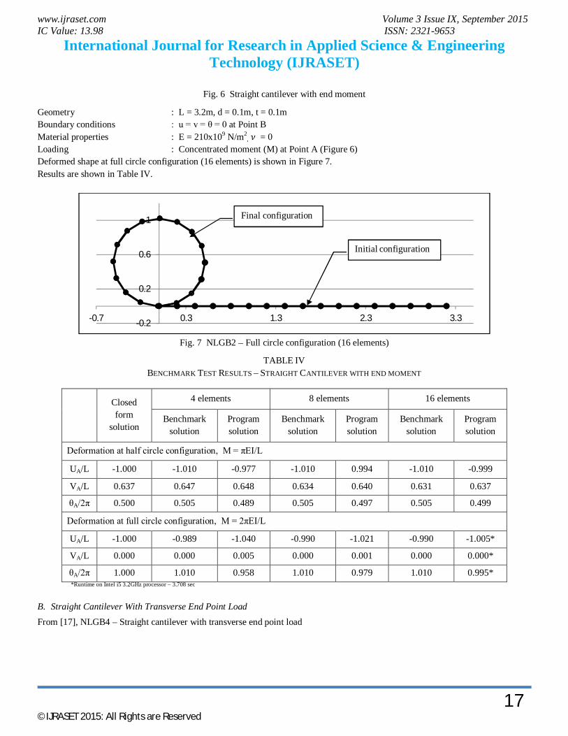
Fig. 6 Straight cantilever with end moment

Geometry : L = 3.2m, d = 0.1m, t = 0.1m Boundary conditions : u = v = θ = 0 at Point B Material properties : E = 210x109 N/m2

, 휈 = 0

Loading : Concentrated moment (M) at Point A (Figure 6) Deformed shape at full circle configuration (16 elements) is shown in Figure 7. Results are shown in Table IV.

Fig. 7 NLGB2 – Full circle configuration (16 elements)

TABLE IV BENCHMARK TEST RESULTS – STRAIGHT CANTILEVER WITH END MOMENT

*Runtime on Intel i5 3.2GHz processor – 3.708 sec

B. Straight Cantilever With Transverse End Point Load From [17], NLGB4 – Straight cantilever with transverse end point load

-0.2

0.2

0.6

1

-0.7 0.3 1.3 2.3 3.3

Initial configuration

Closed form

solution

4 elements 8 elements 16 elements

Benchmark solution

Program solution

Benchmark solution

Program solution

Benchmark solution

Program solution

Deformation at half circle configuration, M = πEI/L

UA/L -1.000 -1.010 -0.977 -1.010 0.994 -1.010 -0.999

VA/L 0.637 0.647 0.648 0.634 0.640 0.631 0.637

θA/2π 0.500 0.505 0.489 0.505 0.497 0.505 0.499

Deformation at full circle configuration, M = 2πEI/L

UA/L -1.000 -0.989 -1.040 -0.990 -1.021 -0.990 -1.005*

VA/L 0.000 0.000 0.005 0.000 0.001 0.000 0.000*

θA/2π 1.000 1.010 0.958 1.010 0.979 1.010 0.995*

Final configuration




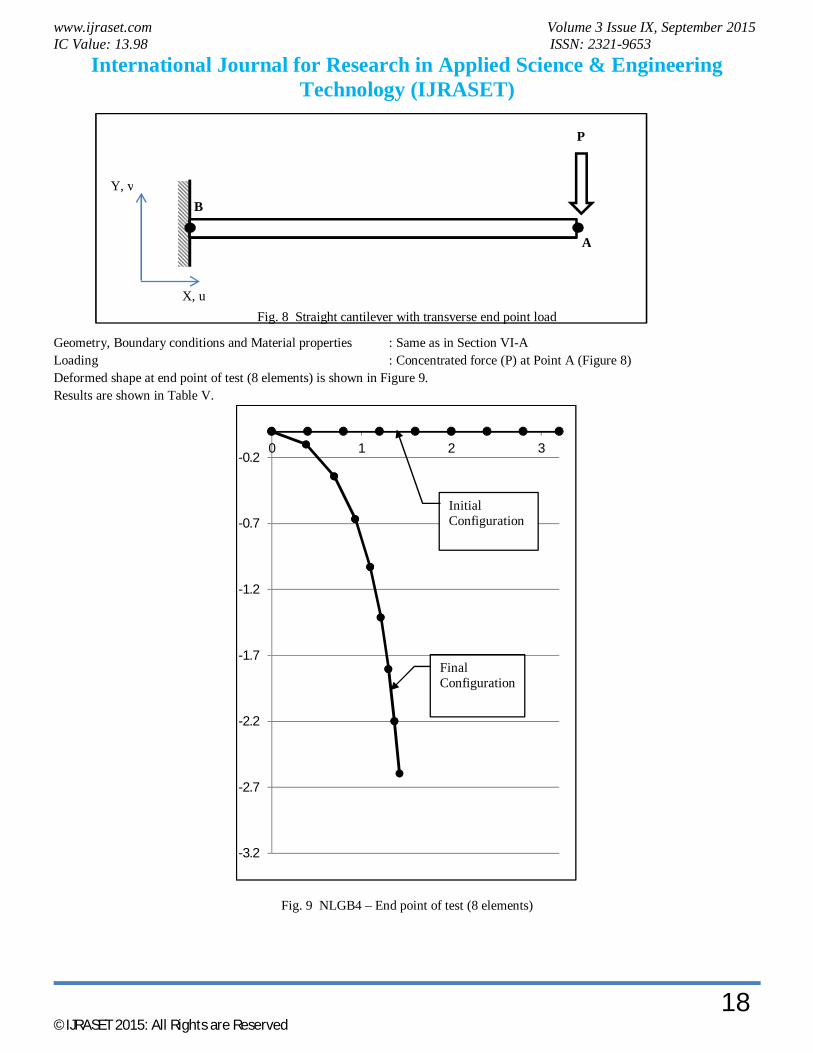
Fig. 8 Straight cantilever with transverse end point load

Geometry, Boundary conditions and Material properties : Same as in Section VI-A Loading : Concentrated force (P) at Point A (Figure 8) Deformed shape at end point of test (8 elements) is shown in Figure 9. Results are shown in Table V.

Fig. 9 NLGB4 – End point of test (8 elements)

-3.2

-2.7

-2.2

-1.7

-1.2

-0.7

-0.20 1 2 3

Initial Configuration

Final Configuration

X, u

Y, v B

A

P




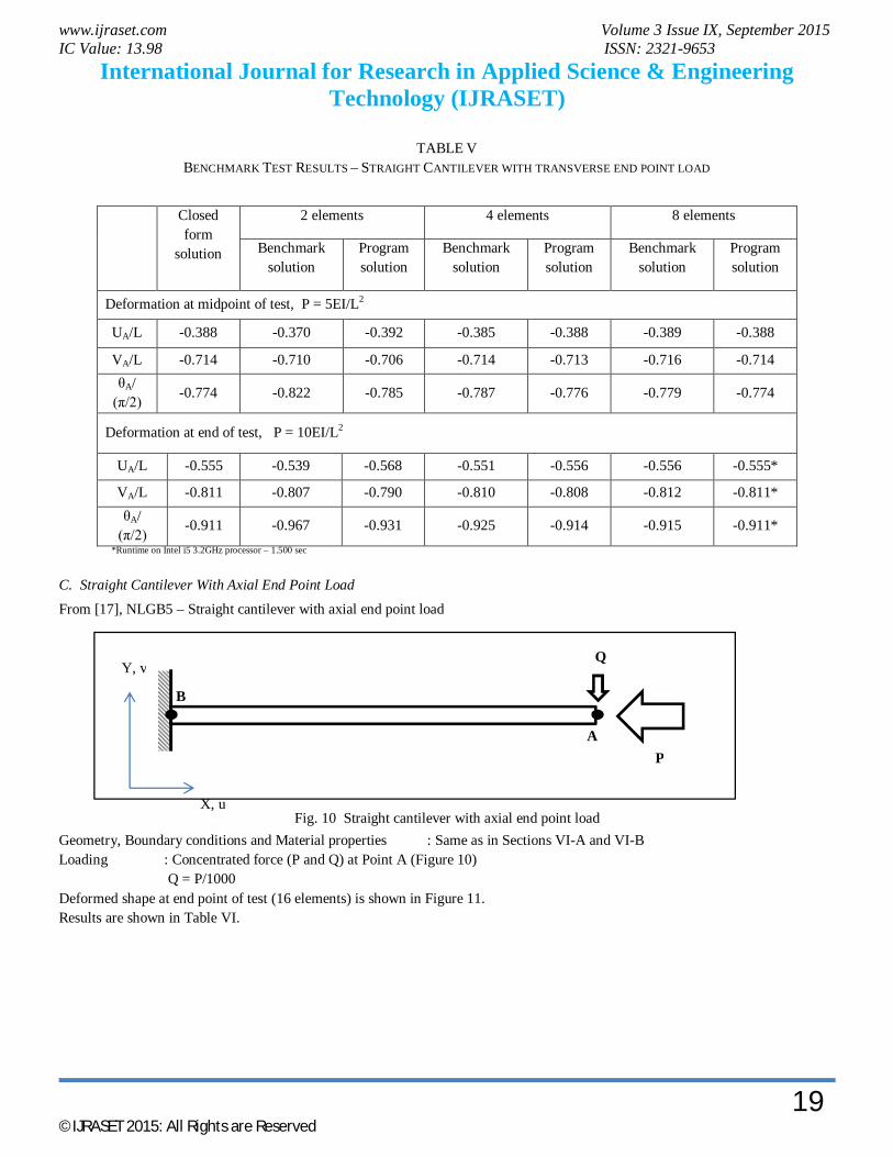
TABLE V BENCHMARK TEST RESULTS – STRAIGHT CANTILEVER WITH TRANSVERSE END POINT LOAD


C. Straight Cantilever With Axial End Point Load From [17], NLGB5 – Straight cantilever with axial end point load

Fig. 10 Straight cantilever with axial end point load Geometry, Boundary conditions and Material properties : Same as in Sections VI-A and VI-B Loading : Concentrated force (P and Q) at Point A (Figure 10) Q = P/1000 Deformed shape at end point of test (16 elements) is shown in Figure 11. Results are shown in Table VI.

Closed form

solution

2 elements 4 elements 8 elements

Benchmark solution

Program solution

Benchmark solution

Program solution

Benchmark solution

Program solution

Deformation at midpoint of test, P = 5EI/L2

UA/L -0.388 -0.370 -0.392 -0.385 -0.388 -0.389 -0.388

VA/L -0.714 -0.710 -0.706 -0.714 -0.713 -0.716 -0.714 θA/

(π/2) -0.774 -0.822 -0.785 -0.787 -0.776 -0.779 -0.774

Deformation at end of test, P = 10EI/L2

UA/L -0.555 -0.539 -0.568 -0.551 -0.556 -0.556 -0.555*

VA/L -0.811 -0.807 -0.790 -0.810 -0.808 -0.812 -0.811* θA/

(π/2) -0.911 -0.967 -0.931 -0.925 -0.914 -0.915 -0.911*

P

X, u

Y, v

B

A

Q




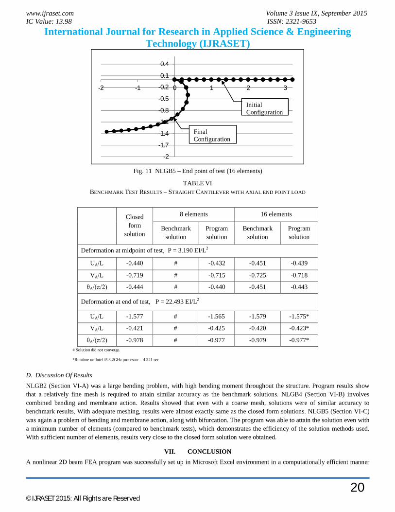
Fig. 11 NLGB5 – End point of test (16 elements)

TABLE VI BENCHMARK TEST RESULTS – STRAIGHT CANTILEVER WITH AXIAL END POINT LOAD

# Solution did not converge.


D. Discussion Of Results NLGB2 (Section VI-A) was a large bending problem, with high bending moment throughout the structure. Program results show that a relatively fine mesh is required to attain similar accuracy as the benchmark solutions. NLGB4 (Section VI-B) involves combined bending and membrane action. Results showed that even with a coarse mesh, solutions were of similar accuracy to benchmark results. With adequate meshing, results were almost exactly same as the closed form solutions. NLGB5 (Section VI-C) was again a problem of bending and membrane action, along with bifurcation. The program was able to attain the solution even with a minimum number of elements (compared to benchmark tests), which demonstrates the efficiency of the solution methods used. With sufficient number of elements, results very close to the closed form solution were obtained.

VII. CONCLUSION A nonlinear 2D beam FEA program was successfully set up in Microsoft Excel environment in a computationally efficient manner

-2

-1.7

-1.4

-1.1

-0.8

-0.5

-0.2

0.1

0.4

-2 -1 0 1 2 3

Initial Configuration

Final Configuration

Closed form

solution

8 elements 16 elements

Benchmark solution

Program solution

Benchmark solution

Program solution

Deformation at midpoint of test, P = 3.190 EI/L2

UA/L -0.440 # -0.432 -0.451 -0.439

VA/L -0.719 # -0.715 -0.725 -0.718

θA/(π/2) -0.444 # -0.440 -0.451 -0.443

Deformation at end of test, P = 22.493 EI/L2

UA/L -1.577 # -1.565 -1.579 -1.575*

VA/L -0.421 # -0.425 -0.420 -0.423*

θA/(π/2) -0.978 # -0.977 -0.979 -0.977*




and benchmark tests were conducted. The program was able to solve problems of large bending, combined bending and membrane action, and problems of bifurcation. Analysis results show that the combination of cubic beam element and CR-TL formulation can deliver very accurate results, provided that the mesh density is chosen appropriately. It is also demonstrated that Microsoft Excel is a convenient platform for setting up such nonlinear FEA programs.

VIII. ACKNOWLEDGEMENTS The author would like to thank Prof. Naresh K. Chandiramani (Indian Institute of Technology Bombay) for introducing him to computer programming in engineering, and Manu Nair (Operations Engineer, SapuraKencana Sdn Bhd, Malaysia) for proof reading this article and providing valuable suggestions.

REFERENCES [1] Lages E.N., Paulino G.H., Menezes I.F.M. and Silva R.R., Nonlinear Finite Element Analysis using an Object-Oriented Philosophy – Application to Beam

Elements and to the Cosserat Continuum, Engineering with Computers , 15, 1999, 73-89 [2] McKenna F., Scott M.H., and Fenves G.L., Nonlinear finite-element analysis software architecture using object composition, Journal of Computing in Civil

Engineering, Vol 24, No. 1, January 1,2010 [3] Commend S., Zimmermann T., Object-Oriented Nonlinear Finite Element Programming: a Primer, Advances in Engineering Software 32, 8, 2001, 611-628 [4] Martha L. Z., Junior E. P., An Object-Oriented Framework for Finite Element Programming, WCCM V, Fifth World Congress on Computational Mechanics,

July 7-12, 2002, Vienna, Austria. [5] M.A.Crisfield, Non-linear Finite Element Analysis of Solids and Structures – Vol 1., John Wiley & Sons Ltd., Chichester, England, 1991. [6] M.A.Crisfield, Non-linear finite element analysis of solids and structures – Vol 2, Advanced topics, John Wiley & Sons, Chichester, England, 1997 [7] Bathe K.J., Bolourchi S., Large displacement analysis of three-dimensional beam structures, International journal for numerical methods in engineering, vol 14

,1979, 961-986 [8] Mattiasson K. and Samuelsson A., Total and updated Lagrangian forms of the co-rotational finite element formulation in geometrically and materially nonlinear

analysis., Numerical Methods of Nonlinear Problems., Swansea, U. K, 1984, 134-151. [9] Hsiao K. M., Lin J.Y. and Lin W.Y., A consistent co-rotational finite element formulation for geometrically nonlinear dynamic analysis of 3-D beams.,

Computer methods in Applied Mechanics and Engineering, 169, 1999, 1-18. [10] Zhang N.W., Tong G.S., A co-rotational updated Lagrangian formulation for a 2D beam element with consideration of the deformed curvature, Journal of

Zheijang University science A, Nov 2008, Vol 9, Issue 11, 1480-1489 [11] Simo J.C., A finite strain beam formulation. The three dimensional dynamic problem: Part 1., Computer methods in Applied Mechanics and Engineering, 49,

1985, 55-70 [12] Simo J.C. and Vu-Quoc L., A three-dimensional finite strain rod model: Part 2: Computational aspects., Computer methods in Applied Mechanics and

Engineering,. 58, 1986, 79-116 [13] Reissner E., On one-dimensional finite-strain beam theory: The plane problem, Journal of Applied Mathematics and Physics (ZAMP), 23,1972, 795-804 [14] Crisifield M.A., A fast incremental/iterative solution procedure that handles “snap-through”,Computers and structures, Vol 13, 1980, 55-62 [15] [15] Ricks E., An incremental approach to the solution of snapping and buckling problems, International Journal of Solids and Structures 15, 1979, 524-551 [16] De Souza R.M., Force-based finite element for large displacement inelastic analysis of frames. PhD thesis, Dept. of Civil and Environmental Engineering, UC

Berkeley, 2000. [17] Holsgrove S.C., Lyons L.P.R., Benchmark tests for two-dimensional thing beams and axisymmetric shells with geometric non-linearity, March 1989, NAFEMS

Report N4

a vba based computer program for nonlinear fea of large displacement 2d beam structures

Documents