a view in ultrasound : analysis of the atl ultramark 9 as ... filebmgt931.139 wfw report nr.93.125 a...

A view in ultrasound : analysis of the ATL Ultramark 9 asa research toolUnger, M.F.

Published: 01/01/1993

Document VersionPublisher’s PDF, also known as Version of Record (includes final page, issue and volume numbers)

Please check the document version of this publication:

• A submitted manuscript is the author's version of the article upon submission and before peer-review. There can be important differencesbetween the submitted version and the official published version of record. People interested in the research are advised to contact theauthor for the final version of the publication, or visit the DOI to the publisher's website.• The final author version and the galley proof are versions of the publication after peer review.• The final published version features the final layout of the paper including the volume, issue and page numbers.

Link to publication

Citation for published version (APA):Unger, M. F. (1993). A view in ultrasound : analysis of the ATL Ultramark 9 as a research tool. (BMGT; Vol.93.139), (DCT rapporten; Vol. 1993.125). Eindhoven: Technische Universiteit Eindhoven.

General rightsCopyright and moral rights for the publications made accessible in the public portal are retained by the authors and/or other copyright ownersand it is a condition of accessing publications that users recognise and abide by the legal requirements associated with these rights.

• Users may download and print one copy of any publication from the public portal for the purpose of private study or research. • You may not further distribute the material or use it for any profit-making activity or commercial gain • You may freely distribute the URL identifying the publication in the public portal ?

Take down policyIf you believe that this document breaches copyright please contact us providing details, and we will remove access to the work immediatelyand investigate your claim.

Download date: 26. May. 2018

https://research.tue.nl/en/publications/a-view-in-ultrasound--analysis-of-the-atl-ultramark-9-as-a-research-tool(27939270-2e6c-48d3-8397-3dcbb0302f86).html

BMGT931.139

WFW Report nr.93.125

A view in Ultrasound

Analysis of the ATL Ultramark 9as a research tool

Michiel F. Unger

Report about practical work project in Baltimore11 April 1993 - 31 July 1993


"Analysis of the ATL Ultramark 9 as a research tool"

By Michiel F. Unger

Preface

The study of biomedical engineering at the Eindhoven University of Technologyincludes two practical work projects. One project I have decided to carry out abroad. Atthe Gerontology Research Center in Baltimore they offered me a research project onanalyzing ultrasound measurements. Using ultrasound is a very interesting way to studythe blood flow in vivo. It is one of the few measuring methods which allowmeasurements without any effect on the biological system.The project helped me to develop a good understanding of this measurement technique.In future blood flow research I will be able to use the obtained knowledge. Also thisproject gave me an opportunity to learn more about practical aspects of carrying out aresearch project. Especially taking measurements on the participants was an interestingexperience. An important difference between the GRC and my university is that theGRC is much more a medical orientated institute which helped me to understand moreabout research in the medical field.I would like to thank the Dutch Heart Foundation for the financial support which reallyhelped me to realize this project. Also I appreciate the help of Arnold Hoeks who sharedhis experience in ultrasound research with me. The Center for Biomedical & Health careTechnology helped me initiating and formulating the project. The great support of mymentor Jeffry Metter and all the helpful people at the GRC made this project aremarkably instructive and an enjoyable experience.

Abstract

"A view in Ultrasound" is the report of my practical work project which is carrie~ out atthe Gerontology Research Center in Baltimore. The objective is to analyze the accuracy ofmeasurements in carotid artery research, using the ATL ultramark 9. The measurementtechnique of the equipment is based on transmitting and analyzing received ultrasoundsignals to measure geometry of the artery and blood velocities in the artery. Importantitems concerning the accuracy of measurements are size of sample volume, homogeneousof sample volume, sound velocity in tissue, quality of frequency analyzer and accuracy ofangle measurement between flow and sound beam.Three experiments have been carried out to study the quality of frequency measurements,sample volume and distance measurements. Some measurements are done to get animpression of the variation in human subjects and the influence of the observer.The ATL ultramark 9 allows a measurement accuracy of distances close to the theoreticpossibilities (accuracy +/- 0.1 rom). Frequency measurements are possible in 1% accurate.The subject variation and the observer have more affect on the measurements. Variationbetween observers can be restricted by good measurement description. Good velocitymeasurements will still show a standard deviation of about 5%.

Contents

1 Introduction 21.1 Why this research? 21.2 Objective of my practical work project 21.3 Introduction in Ultrasound .. . . . . . . . . . . . . . . . . . . . . . . . . .. 21.4 Characteristics in measurements 31.5 Summarized questions . . . . . . . . . . . . . . .. . . . . . . . . . . . . . . . 3

2 Analysis of the measurement system . . . . . . . . . . . . . . . . . . . . . . . . . . . . . . . . . . 52.1 The measurement system . . . . . . . . . . . . . . . . . . . . . . . . . . . .. 52.2 Physics of Ultrasound measurements . . . . . . . . . . . . . . . . . . . .. 62.3 Calculated characteristics according through theory . . . . . . . . . . . 92.4 Causes of error . . . . . . . . . . . . . . . . . . . . . . . . . . . . . . . . . .. 10

3 Experiments for analyzing equipment characteristics..... -. . . . . . . . . . . . . . .. 143.1 Frequency analyzis: signal synthesizer . . . . . . . . . . . . . . . . . .. 143.2 Spatial resolution: String Target 153.3 Depth measurement. . . . . . . . . . . . . . . . . . . . . . . . . . . . . . .. 18

4 Analysis of the physiological system " 194.1 Analysis of variation in physiological measurements . . . . . . . .. 194.2 Explanation of artery image .. . . . . . . . . . . . . . . . . . . . . . . .. 194.3 The best way to measure velocity and geometry 214.4 Review of literature about variation in geometry . . . . . . . . . . .. 22

and velocity

5 Experiments to investigate variation physiological measurements 235.1 Phantom measurements 235.2 Inter sunbject variation measurements . . . . . . . . . . . .. 245.3 Inter and Intra Observer variation 25

6 Discussion6.1 Accuracy equipment and measurement technique . . . . . . . . . . . .. 276.2 Variation in physiological system 276.3 Conclusions 28

SUPPLEMENTS

A Some screen pictures of the ultrasound system.B Test One "Signal Generator"C Test Two "Sample Volume"D Test Three "Depth measurements"E Test four "Phantom and physiological measurements"F Specifications of the Ultramark 9 HDI

Symbol list

Symbol

A =a* =A =IAI =alpha =b =c =c* =err =e =f =fd =fr =lambdam =p =t =T =u =!! =U(i,t) =Vb =Vm =X =Xd =

PI =Rl =CCA =lCA =ECA =PRF =SV =RMS =

ATL =GRC =BLSA =

Explanation

Amplitude of signalestimated aVectorLength of A vectorAngle between beam direction and blood velocityBrightnessSound velocity in tissueEstimated sound velocity in tissueerror parametererror parameterFrequencyDoppler frequencyReference frequency of system= Wave lengthMaterial parameterPower of signaltimeperiod of timevelocityvelocity vectorA function called U depends on E. and tBlood velocityMeasured blood velocityPosition vectordistance from probe

pressur indexResistance indexCommon Carotid ArteryInternal Carotid ArteryExternal Carotid ArteryPuIs repeat frequencySample VolumeRoot Mean Square

Advanced Technology LaboratoriesGerontology Reseacrh CenterBaltimore Longitundinal Study on Aging

unit

m/sdegree

m/sm/s

HzHzHzm

Wssm/sm/s,m/s,m/s

m,m,mm


1 Introduction

1.1 Why this research?

Introduction

Stroke is the third leading cause of death in the U.S. It is primarily a disease of the elderly withapproximately 87% of death and 74% of hospitalizations occurring in those over 65 years of age for1988 [JAMA 1992]. Racial and sex differences, and the higher rates of stroke with increasing age suggestthat the stroke results from a multifactorial process that is not well understood at present [JAMA 1990].Atherosclerosis with thrombosis or embolism in the carotid sinus of the internal carotid artery is the mostcommon cause of stroke. Why atherosclerosis occurs so frequently at this site is assumed to be related tothe anatomy of the sinus and to the blood flow at this point in the artery. It was assumed that the bloodflow causes high shear stresses l~ading to focal injury and subsequently atherosclerosis, however somestudies have found low shear stress at the infected wall zones [Motomiya 1984]. The blood flow in thecarotid bulb is characterized by a helical directional pattern of flow. It is unknown what effects the flowhas on subsequent changes in the arterial wall or with the development of atherosclerosis, or whetherknown cardiovascular risk factors affect the flow pattern.

The Gerontology Research Center (G.R.C.) in Baltimore has planned two related projects to study raceand gender differences in intracerebral arterial velocity and resistance, and blood flow patterns in thecarotid arteries and sinus. These studies will be done as part of the Baltimore Longitudinal Study ofAging (BLSA). The BLSA is a long standing program (started in 1958) that studies normal andpathological aging. Recent interest has developed in factors that may explain racial difference in strokeand health diseases. An ATL ultramark 9, ultrasound machine, has been purchased for collecting data.

1.2 Objectives of this project

Scientists at the GRC would like to know how well the ultrasound machine can be used for theirresearch. The plan for longitudinal studies using this equipment requires that the ultrasound equipment isaccurate and can measure vessel diameter and blood flow velocity consistently over time. The objective isto analyze the accuracy of measurement of the ATL Ultramark 9 ultrasound equipment, and to set upprocedures for measurements in the carotid arteries.

1.3 Introduction to ultrasound.

Sound waves are pressure waves that travel through material with a finite velocity. Ultrasound is soundthat has a frequency above the audible range of man, which is greater than 20 kHz. In both imaging andDoppler applications in medicine, the usual range of the frequency (fr ) is between 1 MHz and 10 MHz.The lower limit is decided by spatial resolution consideration and the upper limit by acceptable powerlevels (attenuation rises rapidly with increasing frequencies). Both ultrasound applications function bytransmitting a beam of ultrasound into the body, and collecting and analyzing the returning echoes. TheUltrasound signal partially reflects at interfaces with different acoustic impedance. If the reflector is smallin respect to the wave length then the signal is scattered. The reflection component gradually decreaseswith increasing frequency. Imaging devices can calculate the coordinates from which echoes originatedand combine this with the power of echo which result in a cross-sectional image from the body. Thebrightness of an image pixel depends on the received power and the distance depends on the time delaybetween transmission and reception. On the machine, adjustments can be made to improve the image butonly the output power adjustment will change the received signal. The adjustments include gain (depthdependent), depth, zoom, grey scale, etc. [User's Manual 1993].

2


PRF = 1 / Tp

fig. 2: The transmitted sound beam.

introduction

Doppler devices can also locate the position of the source of echoes, but the fundamental concern is thefrequency of the returning echoes. If a reflector is moving, a frequency shift (Doppler shift) occurs in thereturning signal. This shift is proportional with the velocity of the reflector. When Doppler shift is foundthen the velocity can be calculated. Slow-moving vessel walls produce high power Doppler signals withlow frequencies. These signals can be filtered with the use of a high frequency pass filter which is calledwall fIlter. Normally a system also contains a low pass filter to eliminate frequencies above thePRF(pulse repeat frequency)/2. Those frequencies are responsible for errors which are a result of aliasing[Hoeks 88]. Today signal analyzers can find the frequencies up to the PRF. In most applications a lowpass fIlter is not necessary. [suggested literature Doppler Ultrasound 1988]

1.4 Characteristics of measurements

The measurement characteristics give information about the quality of measurement and allow a betterinterpretation of the data. The most important characteristics are listed in table 1 [Experimentalmechanics].

IStatic characteristics IExplanation IDuplicity Variation in the measurements which are done in

sequenze

Reproducibility Variation in the measurements which are done inslightly different conditions

Drift Variation in output wilhout change in input

Accuracy Limit of the deviation in measurement

Sensitivity Ratio of change between input and output

Linearity Output linearly dependent on input

Hysteresis Different input can give same output

Stability Change of zero point in time

Resolution Smallest change in input which can be measured

Table I: Characteristics of measurement

3

A view in Ultrasound lmroductioll

It is likely that some characteristics do not play an important part in the Doppler ultrasound system whichis used in this report. The ultrasound technique should minimize drift, hysteresis, instability, and will belinear in velocity and distance measurements. Experiments are necessary to verify these thoughts.

1.5 Summarized questions

This report will try to answer the following questions.

1 What is the measurement performance of the equipment?- What are the characteristics of geometry measurements?- What are the characteristics of velocity measurements?

2 What is the measurement performance of the equipment in physiological measurements?- Is the ultrasound image self explanatory? (Do I see what I think I see?)- What is the best way to measure velocity and geometry?- What are the characteristics of measurements in the physiological system?

In chapter two, an analysis is explained of the measurement system and the ultrasound technique usingthe general theory of ultrasound. In chapter three, experiments are presented to find the characteristics ofthe ATL Ultramark 9. Chapter four presents an explanation of possible physiological measurements and abrief review of measurements found in literature. Results of our measurements are presented anddiscussed in chapter five. In chapter six is discussed the use of this equipment in the research projectwhich is planned by the GRC.

4


2 Analysis of the measurement system.

Analysis of measurement system

Although GRC. scientists are interested in measuring diameter and blood flow velocities the presentedanalysis has a more general pUIpose. With the analysis, I would like to explore the possibilities of theequipment in research on carotid artery. Subjects which are related to the proposed measurements willget more attention. This analysis leads to a better understanding of the system which will help to answerthe question "How well can this machine perform in research studies planned by the GRC scientist?"

2.1 The measurement system

The measurement system consists of three parts:- the subject is the part that will be measured- the equipment is the part that collects data- the observer is the part that has to intetpret the data and to operate the machine.

1.

[ Subject

varl

2.

~U.S. System

var2

fig 3. Black box model of the system.

3.

Observer

var3

The subject is the carotid artery in a human neck. The artery can be described by a volume V which willvary in time. V can be divided in an arterial wall volume Vw(t) and a blood volume Vbet). Using theequipment, certain aspects of the carotid artery can be measured. These measurements will show adeviation with reality. This deviation is caused by the measurement technique and equipment accuracy.The observer wishes to study the wall geometry and the blood velocity field .!!(x,t). material.

* Velocity field equals velocity.!! on every place C!) of volume Vb any time (t)

= .!!C!,t) with .! element Vb,

* Geometry equals material (m) on every place C!) at any time (t).

m

The vessel wall is volume Vwet) in which at every place.! at time t the material is carotidarterial wall (mw).

If the equipment presents vague data readings then the observer could intetpret the data in various ways.Also the observer can operate the equipment differently which could affect the measurements.In short, variation in the measurements comes from the three parts of the system. If the relative variationvarl, var2, and var3 are relatively small the following expression is true.

vart =varl + var2 + var3

5

A view in Ultrasound Analysis of measurement system

The measurement system perfonns well when the variation in observer and equipment is relatively smallin comparison with the variation in the subject.

In the analysis of next paragraph the three parts are considered to be ideal and var2 and var3 are zero.

ideal subject - can be measured in any direction- Tissue in the surrounding of the arteries does not influence the measurement

ideal machine - measures exactly the physical parameters which are used to present the geometry dataand velocity data.

ideal observer - Holds the probe steady during measunnent.- Operates the equipment consistently in time.

2.2 Physics of Ultrasound measurements.

Principles of ultrasound reflection

The equipment transmits a short ultrasound signal. This signal will be partially reflected at interfaces ofdifferent materials. After transmission, the reflected signals will be received. The time (T) of receptiongives infonnation on the distance of source (xd ) and the power (p) contains infonnation on the materialsat the interface.

T depends on the real depth xd• The power p depends on the depth (or the material betweencrystal and reflector) and the reflection coefficient (r) which depends on the material of reflector(m).

p = P(r,xd)

p =P(m,xJr=R(m)

[1]

[2]

Where c is the real average of the sound velocity over a distance xd• As the transmitted signal has acertain length, the received power at time t* can originate from various reflectors in an area with a lengthwhich equals the signal lengths

Principles of Doppler measurements

If the reflector is moving with velocity u, the frequency of the reflected signal will have a Doppler shift.This frequency shift is proportional to the velocity in the direction of the source, sound frequency (fr) and

sound velocity c. Transducer

f r

0/ f r + f d

Bloodflow ---

alphav ::>

SoundbeamfigA.:The effect of a moving reflector on the sound signal.

6


A velocity (Q) results in a doppler frequency (fJ which can be calculated as follows.Vector ! is the direction of the transmitted sound beam.

fd = F<!!.,t;.,!,c)fd= 2 t;. ! ..!L / cfd = 2 cos(alpha) ( I.!!I / c) t;. [3]

When the blood velocity is measured, the received signal exists of a set of signals coming from differentreflectors in the sample volume. As not all these signals have the same frequency, this will not result inone Doppler frequency but in a Doppler spectrum.

Data from the ultrasound machine.

The transducer, which transmits the ultrasound signal, consists of 192 crystals in a row . Each crystal cantransmit or receive an ultrasound signal. This means that the transducer can send and receive only signalsfrom a plane A spanned by the row of crystals and the direction of the soundbeam. The system is capableof measuring the power time and frequency of the received signals. In this analysis I assume that onecrystal only receives the reflections from its own signal. The data to be collected with the ultrasoundmachine consists of:

* Geometry

The machine creates an image of the reflection arriving from a plane (A) under the probe.The system shows at certain coordinates <i*) a brightness (b). What the system measured is:The time delay between transmission and reception (T) and the power of the received signal.(p). The lateral distance is only depending on the physical position of the crystal. From thecoordinates only the distance (xd*=X(i» between probe and reflector is depending on the

sound velocity of the tissue.

xd * = C(T) b = B(p,T)

The function B is not known but xd* is calculated as follows :

xl = c* T c* is the estimated mean sound velocity [4]

T depends on the real depth xd. The power p depends on the real depth and the reflectioncoefficient (r) which depends on the material (m). As different material can producesimilar reflections, it will be impossible to indicate a distinction in materials from a singlereflection. The observer has to decide based upon an analysis of the whole picture.T increases with depth of reflection. Concretely, one measured depth corresponds to one realdepth. Formula 4 and 2 results in:

(1 - c*/c is a measure of the deviation in xd) [5]

Only from plane A, an image of geometry can be viewed on the screen. The equipment only allowsdistance measurements and surface measurements on the screen. Besides the accuracy of measurementand resolution of the machine, errors in the measurements could originate from differences in theestimated sound velocity and the real mean sound velocity.

7


* 2d-Velocity

In plane A the velocity field can be viewed on screen in colour. One colour represents a certainvelocity. The position of the velocity source is calculated similar as the reflector.The sound beam is transmitted in direction! with 1!1=1. The machine calculates the velocityfrom the Doppler frequency (fd ) measurement.

The formula on calculation of the velocity (um2) for a measured Doppler frequency.is derived from formula 3. As the system does not know the angle alpha, it assumes alphais zero (cos(alpha)=l). Instead of the real sound velocity, it uses an estimated sound velocityreflection (c*). This results in the following formula..

The combination of formula 3 and 6 results in

um2 = I.!!I cos(alpha) c*/c

[6]

[7]

According to formula 7, the velocity measurement depends on the angle alpha which is unknown and theestimated sound velocity.

* Point-Velocity

Velocity in a sample volume in plane A is measurable. If the orientation of the plane Ais parallel to the direction of the flow, the angle between beam direction and flowcan be estimated. The formula for the velocity calculation is also derived from 2. Instead ofthe real angle alpha and sound velocity it uses a estimated value (*):

Urn! = 0.5 (fi(fr cos(alpha* )) c*

urn! = 1£1 (cos(alpha) / cos(alpha* )) c*/c

[8]

[9]

Obviously urn! will be closer to the real value of the blood velocity than um2. The accuracy will depend onthe machine accuracy and how close c*, and alpha* are to the real c, and alpha.

Summary

The equipment allows for two dimensional measurements in one plane. Information regarding the thirddimension has to be concluded from external observations. Only distance measurements are possible.These measurements depend on accuracy, resolution and the sound velocity in the tissue. Brightness cannot be measured, but the brightness of a pixel does not indicate much concerning the tissue. This makesunderstanding the image very dependent on the observers experience. The Urn2 measurements provideextra information for an better understanding of the image.The factor cos (alpha) in formula 7 reduces the accuracy of Urn2 measurements. Only urn! measurementsare useful. Velocity measurements are depending on estimated measurement of angle and sound velocityin tissue. To estimate the angle, the observer has to guess what the real velocity direction is. Fortunatelyhe can use the information provided by the image. Of course the frequency measurements will have alimited resolution and accuracy which will affect the accuracy of the velocity measurements.

8


2.3 Calculated characteristics of system.

Geometry

Axial resolution

The length of the sample volume from which signals will be received, relates to the length of theemitted signal. The minimum length of an emitted signal depends on the transducer. Every transducercan emit signals with a frequency in a certain bandwidth (B). The shortest length (T) of a signal isdependent on this bandwidth. The ideal relation between bandwidth and signal length is:

B*T=l [10]

The highest possible bandwidth will be equal to the fr • According to the formula the shortest signallength will be one wave length (Lambda). The reference frequency (fr) in 2D mode is 7.5 MHz.

Lambda = c I fr 'with c = 1540 mls= (1540 I 7,5) 10-6 = 0.20 mm

[ 11]

The axial resolution will be in the order of 0.20 mm. The transducer will not be perfect and probablyhave a larger pulse length.

Lateral resolution.

The lateral resolution depends on the beam width which depends on the crystal size and wavelength[Hoeks 1984]. When the crystal size is small, the wavelength will be the measure of the lateral size ofthe beam. The use of a focal technique can decrease the lateral size of the beam. Normally after a certaindistance the beam will grow wider.

The probe has 192 crystals over a length of 38 mm. Crystal width is 38 I 192 =0.20 mm

This is about the same size as the ultrasound wave length. A resolution of 0.2 mm will be theoreticallypossible with this equipment

Velocity

Spectral resolution

The resolution (pixel width) of a frequency measurement is depending on the sample frequency. If thesystem uses the FFf (Fast Fourier Transformation) technique for signal analyzing then it holds:

F = Sample frequency (= PRF)dF = Frequency resolutiondt = time between two samplesN =Total samples for one measurement

F = 1/ dt= FIN

N *dF =dF

If N and PRF are known, the spectral resolution can be calculated. More information concerning thissubject can be found in [DU 1988, Hoeks 1991]

9


Sample volume size


The sample volume length equals a number of wave length lambda. The system transmits signals with afrequency of 6 Mhz. According to formula [7] these signals have a wave length of .256 mm. The lengthof a 4 wave signal is 1.02 mm. The lateral size of the sample volume is equal to the beam width which isa couple of wave lengths.

2.4 Causes of error in measurements

Distance measurement

Distance measurement errors can occur when measurements are taken in tissue with a significantdifference between estimated sound velocity (c*=1540 m/s) and the real average sound velocity. Withformula (5) the error can be estimated (table 3}.

I Tissue I Sound velocity in mls Max error in % (c*=1540)

Blood 1560-1600 4

Brain 1540 0

Fat 1450 6

Muscle 1580 3

Skin 1600 4

Water (20°c) 1480 4

Average soft tissue 1540 0

Table 3: Error in distance measurements caused by difference in sound velocity in tissue

Angle influence at distance

If a vessel diameter is not measured perpendicularly. there is another error in the measurement. This errorhas to be small in comparison of the resolution (0.2 mm ). The angle may be off err degrees to stay within the measurement resolution. When a diameter of d mm is measured err degrees off from perpendicular,the error in .the measurement is x.

(d+x) = d I cos(err)err = acos (d I (d+x))

x has to be smaller then the accuracy of +1- 0.1 mmA typical value of d is 7mm. According to the formulathe angle err has to be smaller than 9°.

d

ri ... err

II/

- Sample volume reflection

fig.5: Angle influence ondiameter measurement artery

The sample volume wi11limit the resolution of the distance measurements.When the picture is not clear the observer also has to decide where the wall is located. The resolution in

10


time will not influence the measurement because the system allows updates every 0.01 s.

Velocity measurements.

According to formula 9, the velocity measurement depends on the estimated angle and the estimatedsound velocity. The angle has to be measured with the machine, but the sound velocity is already presetin the machine.

Influence of sound velocity

It is possible that the sound velocity in blood changes within a individual. Not a lot of research has beendone in this area. The average sound velocity in blood is 1580 mls [DU 1988] but in [Hoeks 1991] it is1550. Should the maximum sound velocity in blood be 1600 mls [DU 1988] this will produce an error ofaround 4 % in the velocity measurements (C*=1540).

Influence of error in angle estimation

If urnl is measured using the estimated alpha* which is alpha with an error err then the accuracy willbe(derived from formula 9)

Accuracy = (Um-Ume )/urn= l-[cos(alpha+err)/cos(alpha)]

(alpha*=alpha+err)

CGl 15El!!:JenCIlGlE~.<3 100

Q)>.5

gGlGl 5C>19cGl~Gl

Cl.

Angle between vessel and ultrasound beam (degrees)

fig 6: Percentage error in the velocity measurement caused by an error in the angle estimation bctwecnblood flow and soundbeam. A typical angle of 600measured at 10 accurate results in an error inthe velocity measurement of 3%.

11


Spectral broadening


In most ultrasound machines a short (a few wave lengths) sine wave signal will be analyzed as sum ofsignals with slightly different frequencies. On screen this can be seen as a band of frequencies eventhough just one frequency was present in the signal. In different circumstances this band will grow wider,this is called spectral broadening. Many factors influence the spectral broadening, such as.- PRF- Sample volume length.- Blood velocity distribution in sample volume.- Signal processing technique.- Power of signal.- Density of scatters (red blood cells)

Some effects of those aspects of spectral broadening and resolution can be found in [Hoeks 1991, DD1988]. At this point I would like to discuss shortly the result of spectral broadening on velocitymeasurements.Due to spectral broadening one frequency signal will broaden to a band of frequencies. (This changeresult in a I pixel line in the Doppler graph becoming a band of pixels.) When the mean frequency ismeasured, there will be no extra error in the measurement but when measuring peak frequencies thiscould cause problems. Because of spectral broadening the peak of the mean velocity can cover the peakvelocity. Spectral broadening can not be avoided but users should be aware of it.

Wall filters

As explained in the introduction, the wall filters have to filter the lower frequency signals. A badlyworking filter can have a great influence on the velocity measurement. A poor filter will result in anunder estimation (to little filtering) or over estimation (to much filtering) of the mean velocity. A goodfIlter will fIlter all frequencies below a given value and have a narrow band with partial filtering.

Sample volume

All signals coming from the sample volume will contribute to the Doppler signal. The sample volume isnormally described by its axial size. The sample volume length is a number of wave lengths long [DD1988]. The lateral width will be about a couple of wave lengths. In literature the sample volumeresembles a tear drop [DD 1988, Arnolds 1989].Not all signals from the sample volume contribute equally to the spectrum. According to Hoeks [Hoeks1984] the output as function of the position in sample volume should compare to fig.7.

.....;:l r0-:50 1\ A

~AA

~f--)./2 ~X

fig. 7:. Output as function ofaxialposftioh 'ofpoiTir source in sample volume.

12

i view in Ultrasound Analysis of measurement system

According to the graph, one can conclude that signals in the middle of the sample volume make thelargest contribution to the doppler signal. It is possible that a strong source on the edge of the samplevolume will over power a weak signal in the middle. The operator has to know the size of the samplevolume and what is included in the sample volume, for a good interpretation of the data.

13


3 Experiments to obtain information about accuracy.

Experiments for obtaining information about accuracy

Experiments are needed to examine the measurement perfonnance of the machine. I have chosen twotests which were proposed by Dr. A Hoeks from the University of Limburg [Hoeks 1990 ]. The first testanalyzes the frequency analyzing system. the second test is used for analyzing the sample volume. Iadded a third test in which I examine the accuracy in taking depth measurements of the system.In the next paragraphs a short explanation is given of the measurement methods and the results arepresented. Look for a more detailed analysis of the experiments in the supplements.

3.1 Frequency analysis: Signal synthesizer

Purpose of this experiment.

:This experiment investigates the frequency analysis of the equipment. The experiment is proposed by DrHoeks [Hoeks et al 1988]. Infonnation will be obtained on the following items.

a) Characteristics of frequency measurements.b) Reference frequency.c) Wall filtersd) Velocity calculation algorithm.

Method

Results

:A wire connected with a frequency synthesizer is wound around the probe. With themachine we measure (fm) a signal with a known frequency (f.). These frequencies arenear the reference frequency of the machine. The analysis consists of changing the inputfrequency and measuring the output of the system on screen

SensitivityAccuracy

a) Characteristics of measurement

Drift, hysteresis, instability have not been obselVed during the measurementsChanges in input were immediately (within 0.01 s) followed by the output and whenfrequency was set back to the same frequency the result was similar.Measurement resolution - minimum 10 Hz

- .25% of maximum- 100 Hz above 10 kHz- One pixel line has a thickness which is equal to .25% of total scale- Doppler frequencies can be measured with a SD of 1.1 %.

b) Reference. frequency (Fr)

The average reference frequency is calculated using next fonnulafr = l/n ~ ( f. - fm )

= 6,000,061 Hz (SD is 2 Hz)This result is based on 30 frequency measurements.

c) Wall-fIlters

[12]

Three wall-filter settings were tested. By changing the input frequency with increments of 10 Hz the filterquality is studied. Table 4 shows the range of the fIlters, all Doppler frequencies in this range are filteredcompletely.

14

A view in Ultrasound Experiments for obtaining information about accuracy

Wall-filter type fIlters Doppler freq. from to Doppler freq.

25 Hz -20 Hz 30 Hz

50 Hz -30 Hz 50 Hz

100 Hz -100 Hz 110 Hz

Table 4:Wall-filter performance.

All three filters have an overlap between no filtering and complete filtering of 30 Hz.

d) Velocity calculation algorithm

- A measured frequency of 6.25 kHz is equal to a velocity of 80.2 cm/s. This means that the systemcalculates velocities with a sound velocity of 1540 cm/s. (According to formula (2)).

- Angle corrections in velocity measurements are calculated within 1% accurate.

Discussion of results

Frequency measurements are reproducible and duplicable with a standard deviation of 1.1 %. All themeasurements were done mannually on the screen. After the measurements a new mean tracer was buildin the system. This new tool will probably decrease the variation in mean frequency measurements.Calculation of velocities are accurate only differences between the real sound velocity in blood andestimated velocity (1540 m/s) can give extra errors. The wall-filters performs well, low frequency«500Hz) measurements have a poor resolution.

3.2 Spatial resolution: String target

Purpose of experiment

This experiment investigates the axial and lateral size of the sample volume. Both the sample volumes ofdoppler system and imaging system are studied.

Method:

Results

An oscillating string is moved through the sample volume of the Doppler system in awater vessel. The string is moved horizontally and vertically through the middle of thesample volume which has highest output. The string direction is perpendicular on theplane of measurement. The headphone output is measured with a RMS-Volt meterThe wire oscillates at 600 Hz and the wall filter is set at 300 Hz.

- Sample volume of reflection

The hair has a diameter of 0.04 mm which is much smaller than the sample volume of the reflectionmeasurement. The image of the hair on the screen gives an good idea of the resolution. In fig.8 you seethe hair willi the system on maximum zoom. It is possible to see a square in the centre of the bright spot(0.2 mm by 0.2 mm) which represents one pixel of the image. The system uses a correction on the screento make the picture look smoother.

15


fig. 8:

Hard-copy of screen picture from hair inmaximwn zoom mode. The bright spotis a cross-sectional image of the hair.Axial movement can be measured in 0.1mm accurate. Lateral movement can bemeasured 0.2 mm accurate.

- Sample volume of velocity measurement.

Experiments for obtaining information about accuracy

The output is measured on different axial positions of hair in sample volume at depth of 10 mm, 20 mmand 40 mm. The sample volume length was preset to Imm on the ultrasound machine. In the graph 9,10and 11 the output ratio is defined as output / maximum output.

fig. 9:Output ratio as function of the axialposition of the hair in the samplevolume. The sample volume length isdependent on the definition of thislength. A reasonable defmition is thelength where more than 10% ofmaximwn power is reflected.

1.1

1.0

0.9

0.8

20.7

2 0.6

:; 0.5.9-co 0.4

00.3

0.2

0.1

0.0

16

So~ple VOlumeAxial size of 1mm SV ot 10,20,40mm

<

I

i,l,,

"

,,

0.0 0.2 0.4 0.6 0.8 1.0

-+ X Axial size in mm

10mm20mm40mm

I'I

I

II

\'\I , ,

\ .~./ \-

1.2 1.4 1.6. 1.8

A view in Ultrasound Experiments for obtaining illformation about accuracy

Also the output ratio is measured on different lateral positions of hair in sample volume

Sample ''/oiumeL~teroi size cf 1m~ ':;"/ ct 1O.20.4Qmm ce:::'r..

fig. 10:Output ratio as function of the lateral (L)position in the sample volume. Thepositions of maximum output of thethree measurements are put on positionzero.

, ~

I.v

0.9

O.B

:-: 0.70

G.50

.C::: 0.5

a. O.L

6 0..3

C.2

C.

1\..l" ,-\

I, .., ', . ,

;:. ....

, ', ',

:!__ -/:J/ .

---"--

-~ -;- 0---~iI' L _::e':' ::s:c~:e '" "'''''

,,

40mm20mm10mm

Three different sample volumes with a length of 1, 3, 5, 7.5 mm according to equipment are measured.The middle of the sample volume is put on a axial distance of 20 mm.

Samole volumeAxial size 1 mmSV

3 mm SV5 mm SV7.5 mm SV

fig. 11:Output ratio as function of the axial (X)position of hair in the sample volume.The sample volume of 7.5 mm looks tobe only 5.5mm long. (10% definition)This is more than 25% smaller.

Discussion of results.

1.0

0.9

0.8

0.70.~ 0.5~

:; 0.5a.

" 0.40

0.3

0.2

0.1

0.0

0 2 3 4

o·_.-. ----{3---

5 5 7

Sample volume of the Doppler system--.... X Axial size in mm

Looking at the results of the experiment it can be concluded that the sample volume is smaller than thegiven value by the manufacturer. Although it is not determined what the length of the sample volume is.A reasonable description of the border line could be that at the border 10% of the maximum power willbe received. Regarding this description, the measured axial size can differ morc than 25% of the sizeviewed on screen. This difference can not be caused by the measurement errors. Also the axial size isdepth dependent. I have not an explanation for these facts. Only the lateral size is almost independent ofthe length of sample volume and depth. For as long as the sample volume is in focus.As expected the reflections coming from the centre have the largest contribution to the Doppler signal.

17

A view in Ultrasound Experiments for obtaining information about accuracy

The smallest sample volume (1 x Imm) is rather large for a detailed blood flow study..When the averagevelocity has to be measured, the conclusion will be to use as large a sample volume as possible. Becausethe blood velocity in the middle of the vessel (sample volume) has the highest velocity (largestcontribution to the Doppler signal) the average velocity will be overestimated. A larger sample volumereduce the affect of the in homgeneous of the sample volume.

Sample volume imaging system

Spatial resolution of the imaging system is 0.2 mm by 0.2 mm. Changes in lateral position can bedetected with 0.2 mm accuracy. Axial movements can be followed more accurate but the system allowsonly measurements with an accuracy of 0.1 mm. Two close reflection sources can appear as one becausethe image has been smoothed.

3.3 Depth Measurement

Purpose of experiment

Most vessel diameters will be measured by measuring an axial distance. With this experiment it ispossible to find the accuracy in measuring depth and axial distances.

Method

Results

: Between a reflector and the probe a spacer is fit with an precise height. Thedistance between probe and reflector is measured. The error is the difference betweenheight calculated from block heights and measurement. The depth can be changedthrough placing small spacers on the reflector. Every measurement is duplicated twiceand reproduced twice.

With the spacers 18 different depth measurements were possible.~--------------------------.

o

- measl real··0 meas2real

- -. - meas1 cor---{3--- meas2 cor

o

•••

Depth in mm

•o

o

Error in depth measurements

1.8

1.6

1.4

1.2

1.0

0.8

0.6

0.4

0.2

0.0

-0.20:--~--:1"'::O--~2~O---J--'-O---4..LO-~---J50

EEc

2W

Discussion of results

fig. 12:Error in depth measurement as functionof the real depth according to thespacers. The corrected depth has acorrection for the difference in soundvelocity in tap water (+1- 1480 m/s) andtissue (1540 m/s).

Depth measurements are goodreproducible and duplicable. The errorin the measurements seems to beproportional with the depth. The resultsare duplicable at 0.1 mm accurate fordepth lower then 30 mm andreproducible at 0.2 mm accurate. The machine overestimates the real depth by 4.6 %. The velocity inwater is about 4% lower then the average velocity in the human body. So the accuracy of the averagedepth measurement is around 0.6 % of the depth.,but the sound velocity in our tap water was not exactlyknown. The standard deviation in all depth measurements until 40mm was 0.1 mm.

18


4 Analysis of physiological measurements

4.1 Analysis of variation in physiological measurements.

Analysis of physiological measurements

As mentioned in chapter two there are three parts which contribute to the variation in the measurements.Variation in the measurements can be split in to the following groups:

1 subject

2 Measurement method variation3 observer

la Inter-subject variationlb Intra-subject variation

3a Inter-obseIYer variation3b Intra-obseIYer variation

In the second and third chapter the variation in measurement technic and equipment is analyzed. In thischapter I would like to explain more about the way physiological measurements can be done. Thisfollowed by some experiments which are carried out to give an impression of the subject and obseIYervariation.

4.2 Explanation of artery image

There are differences between reality and images. According to chapter two one bright spot on the screendoes not tell a lot about an artery. A combination of bright pixels can give you a better idea of the artery.The artcry image can cause difficulties for a number of reasons.First, the artery has to identified. The easiest way to find the artery is cross-sectional where the artery canbe viewed on the screen as a pulsating circle with a dark nucleus (fig 13). When the artery is straightand measured longitudinal, two parallel walls can be noticed on the screen (fig l4).Thc sound beam hasto be perpendicular on the artery, giving the best pictures..

fig. 14.

If you measure the artery diameter in a different angle than 90 degrees, the arterial wall will be vagueand the picture could look elliptical. Should you see the artery at the bifurcation (fig 15) or when thearteries are cUIYed it will be difficult to reconstruct the three dimensional geometry of the artery of a twodimensional image.

19


i.c.a.

1111111c.c.a.

fig 15: A carotid bifurcation.


When you have a good picture of the wall, it is possible to identify three lines [O'leary 1991]. Theselines correspond with three interfaces (fig 16).

1 - Intima-Lumen2 - Adventia-media3 - perieadventitia-adventia

Artery~Advc:ntia

Media---- Intima

1~ _

~/fig. 16: Arterial Wall

Checking through some literature regarding the carotid arteries the following statements were madeconcerning the geometry of the bifurcation.

According to Camilo Rindt (1989) the common carotid is not circular. Two perpendicularmeasurements of the diameter showed a difference of 10 %.

In most articles the artery is modelled to be circular.[Baia 1979, Forster 1985]

The bifurcation looks like to be laying in one plane. [Camilio 1989. Balas 1979].

20


4.3 The best way to measure velocity and geometry


As mentioned before there are two ways of creating images which can be used in making measurements.One way is longitudinal and the alternative is cross-sectional on the artery. Both ways have advantagesand disadvantages.

Geometry

Diameter

Diameter can be measured longitudinal or cross-sectional. According to Hoeks measurement of the arteryin longitudinal direction is better because the wall irregularities can be easier detected. Cross-sectional iseasier and gives you an idea of the circularity of the artery. I have tried to use both ways of measuring.Most reproducible measurements are measuring the minimum distance between the walls on alongitudinal picture.The advantage of using the M-mode (Supplement A) is that the minimum and maximum are easier torecognise. But no wall irregularities are detectable.

Angle

To measure the angle of a bifurcation, you have to obtain a picture of the bifurcation. After which it ispossible to measure the angle on the screen or hard copy.

Velocity

If highest accuracy is required, two independent measurements are necessary for geometry and velocity.To measure the absolute velocity one needs to know the angle of measurement within one degreeaccurate and the angle should be under 70 degrees.Only in case of longitudinal measurements is it possible to measure the angle accurately enough. Errorsare introduced by a changing angle during a heart cycle and also the assumption that the blood flow isparallel with the wall.When the imaging plane is perpendicular to the vessel (cross-sectional direction) you can not measure theangle but it can allow you to measure with a smaller angle. Should the observer only be interested in theindices (formula 13,14} then no angle correction is necessary.

PI

RI

=Ipeak sys. vel. - end sys. vel. I / Imean veLl

=Ipeak sys. vel. - end sys. veLl / Ipeak sys. veLl

[13]

[14]

Measuring this way only ratios of the velocity can be used like the Rl and the PI. A smaller angle givesa better doppler signal. The gain and power adjustments could influence the peak velocity. It isimportant to use lowest gain and power as possible to get a reproducible peak velocity line.The ATL Ultramark 9 is able to measure automatically the mean velocity and peak velocity. Theequipment also generates time averaged (t.a..) peak velocity, t.a. mean velocity, end systolic velocity, PIand RI from heart beat to heart beat. I have studied the variation in these values and the arterialdiameters of the common carotid artery.

21


4.4 Review of literature about variation in geometry and velocity

Geometry


In the following table is a summary of the literature regarding measurements of the geometry of carotidarteries. When available the s.d is included.

IReference II d. cc Id. IC Id. EC IBA IN IAge IMT IForster 1991 7.8-.99 5.5-1.1 4.1-.99 53.6-10 34 54 A

Merode 1988 6.3-.65 - - - 95 42 US

Hoeks 6.2-0.5 - - 10.8-5.2 11 25 US

6.4-1.0 - - 12.6-3.5 9 55 US

Hoeks (inter) 7.1-0.05 - - - 5 US

Mortes. 1990 6,8-.93 - - - 20 41 USRight side

Left side 6,7-.79 - - - 20 41 US

Table 5:Diameters and errors from the literature. d = diameter, CC=Common carotid, IC=Intemal carotid,

EC=extemal carotid, BA=Bifurcation angle, N=number of measurements, Age= average age, MT=Measurement Technique (A=angiography,US=U1trasound)

As one can conclude from the table above the variation in diameter is rather large.

Velocity

Not much data was available about the variation of the blood velocities. The next table summarized someof the data. The variation between the measurements is remarkable.

I reference II flow interval In Iage IFuiji. 1982 6.9-10.4 mVs 140 10-79

Uematsu 1982 6.5-8.7 mVs 120 21-60

Mulle 1984 7.1-8.6 mIls 100 16-65

Sugi 1985 6.8-9.9 mIls 60 21-69

Sawai 1987 6.6-11.4 mIls 108 30-79

Table 6 The flow interval is a 95% confidence interval.

22

A view in Ultrasound Experiments to investigate variation in physiological measurements

5 Experiments to investigate variation in physiological measurements

The BLSA is especially interested in changes within an aging individual. In the literature I have notfound enough articles about the variation of ultrasound measurement within an individual. Probably thechanges are small and the question is how many measurements are necessary to tell with a reasonablecertainty if there is a difference. With the following experiment I try to find the variation within anindividual and the influence of the observer on the measurements. Because of time limitation of mypractical work the number of measurements are very small. Still they give a reasonable idea of thevariation. If more accurate data is needed more measurements have to be taken.The experiment consists of phantom measurements, inter-subject variation measurements, and intraobserver variation measurements.

5.1 Phantom measurements

Purpose

The string velocity of the phantom is very good reproducible. Also it is possible to give the string avelocity pattern which is similar with blood flow patterns in the common carotid. Using this experiment,one can study the variation in the measurement of the velocity parameters on a constant subject.

Method

The phantom consist of a string which moves through water. The velocity of the string is precisely (+/- 1cm/s) known and the string velocity is measured with the ultrasound machine. In five differentconfigurations 20 times the value of peak vel., mean vel., time averaged (t.a.) peak vel., end systolicvel., PI and RI are collected. Every measurement configuration has a different measurement angle.

Results

First, the string speed is set at a constant speed of IJ)Ocm/s. With the equipment the mean velocity andpeak velocity are measured. The difference in those velocities gives an idea of the noise in the system.Then the phantom is set for common carotid simulation and the different velocity parameters aremeasured. The results are the mean and the standard deviation of 20 measurements

IAlpha II66 I62 158 1

50 IPeak (V=I00) 131-3.5 120-3.2 126-1.8 119-1.5

mean (V=I00) 67.5-2.6 96.5-4.6 94.5-3.5 100-1.5

peak sys. (V=95) 116-5.8 115-4.3 115-8.2 109-3.9

end sys. 33.4-5.5 36.2-3.4 34.4-3.2 32.8-2.4

t.a.mean (26.7) 20.7-1.1 27.5-1.8 27.8-1.0 26.2-0.84

t.a. peak 47.6-2.1 47.7-2.5 44.8-1.9 44.4-1.5

P.I. 2.73-0.38 2.73-0.38 2.76-0.40 2.81-0.28

R.I. 1.14-.039 1.14-.060 1.16-.033 1.15-.042

Table 7: Results of phantom measurements.

23


Those measurements were performed in sequence. These measurements are well duplicable, but they arenot well reproducible especially the constant speed measurements. The measurement under 66 degreesproduced a lot of noise which probably influenced the measurements accuracy. Another problem was thescreen. When a video tape with the measurements is played, it is difficult to distinguish the 3, 5, 6, 8,and 9.

Conclusions

The received Doppler signal is rather noisy resulting in a wide frequency band on the screen. This broadband causes the peak velocity measurements to have a poor (error more 25 %) accuracy. The meanvelocity measurements are much better, but at times this is very poor too. The string which is usedconsists of surgical silk. This silk wears out rather quickly when it is used on the phantom. One problemis that the results of the measurement can change during the wear process.The values best reproducible and accurate to the true value are mean velocity and the PI and RI. Peakvelocities showed too much variation. Still the measurement variation is too large for more detailedanalysis. The phantom is too noisy maybe a different string will help. The noise is probably a result ofthe string source which reflects many coherent signals.

S.2 Inter subject Variation measurements

Purpose

I would like to study the variation of diameter and velocity measurements within a individual and if thisvariation is similar between different individuals. This information could be used to answer the questionhow many measurements do I have to perform to obtain a good result?

Method

Diameter

The diameter of the left common carotid is measured. On a longitudinal image the diameter is measuredin the M-mode. In the M-mode the image of one line is dislpayed as function of time (Supplement G).Adjustments have been made to view the wall reflection lines as narrow as possible. At first the imageshave been recorded on video tape. Measurements took place during replay in calculation mode. Themeasurement crosses are placed just in the reflection line, moving away from the middle of the artery.The minimum and maximum diameter is measured 5 times (different heartbeats) at more than 10 mm ofthe bifurcation.

Velocity

Also in the left common carotid the velocity is measured in the middle of the artery with two differentsample volumes (SV 1 mm, and the averaged velocity over the whole artery SV 7.5 mm). Fourindividuals have been measured. Within the individual the velocity parameters have been measured 10times in sequence. The angle correction on the machine is used. All measurements have been done byone obseIVer in a similar way. First, the pictures with the measurement values were recorded, later thesevalues are collected and processed.

Results

The results are summarized in the following tables. In every table the mean value is given and also thestandard deviation

24


ISubject number I Minimum diameter Maximum diameter Diameter change

1 5.20 (.00) 5.68 (.04) 0.48 (.046)

2 4.69 (.05) 5.50 (.07) 0.54 (.054)

3 6.26 (.05) 6.80 (.10) 0.54 (.054)

4 4.60 (.07) 5.35 (.10) 0.74 (.054)

5 4.60 (.00) 5.02 (.10) 0.42 (.084)

Table 8: Common carotid diameter measurements in mm and (standard deviation).

The next table summarized the velocity measurements in the left common carotid of four differenthealthy people. The participants consisted of two men and two women between 25 to 65 years of age.The values are the mean values of all measurements ( 4 times lmm SV, 4 times 7.5mm SV).

Peak sys. t.a. mean vel. t.a peak. vel PI RI

mean (SD%) 105 (10.1%) 27.6 (13.1 %) 42.2 (18.5%) 1.95 (20.2%) 0.79 (3.94%)

Table 9: Intra subject variation in velocity measurements in cmls and (standard deviation in %)

When the standard deviation within each subject is derived through the mean value, the relative variationin the measurements between the subjects can be compared. Table 10 gives an impression of the variationwithin the subjects.

Peak sys. t.a. mean vel. t.a. peak vel. PI RI

mean sd 4.44 4.23 3.73 7.08 5.14

Table 10: Average value of inter subject standard variation in %.Conclusion

Diameter measurements, including diameter changes, are good duplicable. Difference between inter andintra subject variation is clear. Measurements are possible with a standard variation of less then 0.1 mm.Velocity measurements showed more variation in both small and large sample volume. The measurementsusing the 1 mm sample volume show little less variation, all though differences are small. Mostreproducible appears to be the peak velocity, t.a. mean velocity, t.a. peak velocity and RI which have ainter subject variation of 5%. A part of the inter subject variation can be explained through a slightchange of measurement angle. A one degree angle change gives at 60 degree 3% variation. The intrasubject variability is rather large in every parameter except the RI.

5.3 Inter and Intra Observer variation.

Purpose

Every observer executes the measurements slightly different. In this experiment I will study what theeffects are of different probe positions on the results. I would like to compose the most suitable place andposition for velocity measurements.

25


Method

Of one healthy participant the velocity parameters are measured at two different positions. In everyposition the measurements are done ten times in a row. The measurements are done in the left commoncarotid. At each place the angle between the probe and vessel is varied between the different sets ofmeasurements. The distance between transducer and carotid bifurcation (1) is measured with an accuracyof 4 mm. The angle alpha is measured using the features of the ultrasound machine which allow angleestimation with the highest accuracy of I degree. When measurement was cross-sectional no angle ismeasured.

Results

The results of the measurements are summarized in next two tables. The table II shows the relativestandard deviation of every measurement set and the mean of the relative standard deviations. Table 12contains the mean value and SD of the 6 measurement sets.

ry

II -alpha I peak veL t.a. mean veL t.a. peak PI RI

20 - 68 0.0091 0.0438 0.0256 0.0885 0.0759

20 - 52 0.0747 0.0538 0.0427 0.0661 0.0165

40 - 70 0.0493 0.0525 0.0364 0.0621 0.0230

40 - 56 0.0234 0.0436 0.0767 0.0714 0.0237

40 - 46 0.0405 0.0420 0.0923 0.120 0.0985

40 - cross 0.0660 0.0642 0.1035 0.0809 0.0228

I mean II 0.0440 I0.0500 I0.0629 I 0.0816 I0.0436 ITable 11: Relative standard deVIation of eve measurement set.

peak sys v. t.a. mean veL t.a. peak vel. RI PI

mean value III* (15.7%) 21.6* (11.5%) 35.9* (18.3%) 2.50 (8.53%) .815 (2.80%)

Table 12: Mean value and standard deviatIOn of all measurement sets.(>/<'- without 4U-cross measurement)

Some remarks regarding the measurements:

20-68 Some peak velocities have been affected by PRF which was to low.40-46 To measure at this angle the you have to use some force which may influence the flow.

Conclusion

The results show a variation in the velocities values of more than 18% between the differentmeasurement position and orientation. From all the parameters the RI, PI and time averaged meanvelocity are the best reproducible. The variation within one set of measurements is similar with the interintra subject measurement. Variation in a measurement set is mostly about 6%. More practice willprobably result in a better reproducibility of the measurements. From this experiment no clear conclusionscan be extracted to locate the best position and angle.

26


6 Discussion

6.1 Accuracy equipment and measurement technique.

Geometry

Discussion

The machine can measure vertical distance at 0.1 mm accurate when the distance is below 30 mm. Incase of carotid arteries this is sufficient. For the calculations of distances the machine uses a soundvelocity of 1540 m/s. In certain tissues the sound velocities can differ significantly of 1540 mls whichresults in errors of about 4%..

Velocity

The tests showed that the equipment can find the Doppler frequency within 1%. The signal analyzingprocedures seems to fulfil its purpose well. Only the size of the sample volume is smaller than thesuggested size. The operator should be aware also that signals originate from the middle of the samplevolume have the largest contribution to the Doppler spectrum.According to the theory, velocity measurements are highly dependent on the angle correction. The anglecan be measured in one degree precise. This produces an error of 4% in the measurement. The smallerthe angle the smaller influences in the estimation error. Errors caused by differences in sound velocity inblood could be about 4% but in most cases the sound velocity is not known.

6.2 Variation physiological system.

Geometry

To obtain a good diameter measurement the operator should have a clear picture of the artery. The Mmode of the system gives the best opportunities to find the minimal and maximal diameter. On the screenthe reflection line of the wall should be made as narrow as possible and maximum zoom should be used.Then it will be possible to get a reproducibility and duplicability within 0.2 mm. Only measurements inone plane are possible, the observer can add a third dimension by using his sense-organs. Measuringcomplex 3D structures is very difficult using this method and will be highly dependable on the observerwho does the measurements.In more sensitive measurements, the result can be significant different between observers and even withinone observer. One reason could be the items to be measured are not good visible so the observer has toestimate, for example, where the vessel wall begins or disappears. Especially when the diameter of theinternal or external is measured, the wall is mostly difficult to see or even invisible.

Velocity

Velocity measurements show more variation than the geometry measurements. A good description shouldbe available for each measurement. The built in peak tracer and mean tracer should be used together withthe calculation possibilities of the equipment. This will result in variation of about 5% in the results.Theobserver variation will be relatively small in comparison to the subject variation. Although it will be verydifficult to distinguish the observer variation from the subject variation. Without paying much attention tothe measurement there can be a variation in the results of more then 15%. The observers skill inmeasuring with steady angle will be the main influence in the measuring.

27


6.3 Conclusions

Discussion

The ATL Ultrasound machine allows reproducible and duplicable measurements. Although themeasurement technique and subject makes it difficult to get reproducible and duplicable velocitymeasurements. Diameter measurements of the common carotid show good measurement characteristics. Inother carotid arteries the wall is more difficult to see that makes the measurement less accurate. Probablya lot of practice and a good measurement description will minimize the variation. Also the usefulnessdepends on the requested measurement accuracy.The view with ultrasound is not quit clear yet, but its much better than having no view at all.

28

References

K Balasubramanian, An experimental investigation of steady flow at an artificial bifurcation,thesis 1979.

D.H Evans, W.N. Mc Dicken, R. Skidmore, J.P. Woodcock, Doppler Ultrasound, 1988.

F.K Forster, P.M. Chikos, lS. Frazier, Goemetric moddeling of the carotid bifurcation inhuman implications in ultrasonic Doppler and Radiologic investigations, Ultrasound 13, pp.385-390 July/August 1985. .

Camilio Rindt, Analysis of the three-dimensional flow field in the carotid artery, 1989.

A. P. G. Hoeks, Tecnology in ultrasound diagnosis, Ultrasonoor bulletin 2-1988.

A. P. G. Hoeks, C. 1. Ruissen, P Hick, R. S. Reneman, Methods to evaluate the samplevolume of pulsed Doppler system, Ultrasound in Medicine Vol. 10, No.4, pp. 427-434, 1984.

A. P. G. Hoeks, Spectral composition of Doppler signals, Ultrasound in Med. & Biology, Vol.17, No. 18, pp. 751-760, 1991.

A. P. G. Hoeks, Are flow models necessary to evaluate Doppler systems, Ultrasonoor bulletin,1-1990.

A.P.G. Hoeks, P.J. Brands, F.A.M. Smeets, R.S. Reneman, Assesment of the Distensibilityof superficial arteries. Ultrasound in Med. & Biology, Vol. 16, No.2, pp. 121-128, 1990.

K Howi, S. MOchio, Y. Isogai, Y. Miyamoto, N. Suzuki, Comparison of color flow and 3dimaging by computer graphics for the evaluation of carotid disease, Angiology, april 1990.

T. van Merode, P.J.I Hick, A.P.G. Hoeks, F.A.M. Smeets, R.S. Reneman, Differences incarotid artery wall properties between presumed healthy men and woman, Ultrasound in Med.& Biology, Vol. 14, No.7. 1988.

J.D. Mortensen, S. Talbot, J.A. Burkart, Cross-sectional internal diameters of human cervicaland femoral blood vessels in relationship to subjects sex, age, body size. The anatomicalrecord 225: 115-124, 1990.

D.H. O'Leary, J.F. Polak, S.K. Wolfson..., Use of Sonography to evaluate carotidatherosclerosis in the elderly, (The cardiovascular health study), Stroke, Vol. 22 No 9September 1991.

Users' Manual ATL ultramark 9 HDI, ATL 1993..

JAMA 1992, Cerebrovascular disease mortality and medicare hospitalization-United States,1980-1990, 268:858-859.

JAMA 1990, RJ. Kittner, L.R. White, KG. Losonczy, P.A. Wolf, J.R. Hebel. Black-whitedifferences in stroke incidence in a national sample. The contribution of hypertension anddiabetes mellitus, 264:1267-1270

Supplement A

Some screen pictures of the ultrasound system.

Picture 1:

Picture 2:

Screen picture of hair in maximum zoom. On screen can be seeen inthe middle a bright square (0.2xO.2mm).

Screen picture of Doppler measurement of vibrating hair. In the Dopplerspectrum appear two lines (600 and -600 Hz) which equals the vibrationfrequency. In the right column are the settings like PRF. frequency,angle correction, etc.

Picture 3: The changing diameter of common carotid in M-mode. The movementof the walls can be followed very well.

IMAGE DOPPLER SPECTRUM

Picture 4: Screen picture of common carotid measured in Duplex mode. In theimage the place of the sample volume can be seen and also thecorrection for the angle. In the doppler spectrum you can see thedifference between two heartbeats. In the column at the right are theresults of the measurements. These numbers change with every beat.

Supplement B

Test one

Title :Signal generator

Purpose :This experiment investigates the frequency analyses of the equipment. Theexperiment is proposed by Dr Hoeks [Hoeks et al 1988]. Information willbe obtained on the following items.

Method

a) Characteristics of frequency measurements.b) Reference frequency.c) Wall filtersd) Velocity calculation algorithm.

A wire connected with a frequency synthesizer is wound around the probe. Thesynthesizer generates a high frequency signal.( Fs ) which the ultrasound equipment canmeasure. The output of synthesizer is regulated in a way that it give as narrow band aspossible on the screen of the ultrasound equipment. The frequency is measured ( Fm )

manually in the middle of the band on the screen. Different synthesizer frequencies aremeasured with the equipment

a) ResolutionDynamic responseAccuracy

- Smallest measureble frequency change.- Response time of system after ending the signal- From ten different frequency signals the mean frequency is

manually measured three times. This frequency iscompared with the Dopplerr frequency which is calculatedfrom the reference frequency and counter frequency

Results are investigated on possible hysteresis, drift and instability

b) Reference frequency can be calculated as follow, using the measurement data

(1)

c) Through changing the synthesizer frequency with increments of 10 Hz, the 25, 50and 100 Hz wall filters are studied. The measured range coveres the filter range

d) The estimated sound velocity (c*) can be found when the velocity scale is used.The sound velocity can be calculated with the use of fr , fs' U m and

c* = 2 Om fr / (fs-fr ) (2)

- HP 3320A- +/- 50 Turns- HP 53268 (accuracy 1 Hz)- ATL-Ultramark 9 HOI- ATL LIO-5

Equipment :-frequency synthesizer to 1 to 10 MHz-Wire-Frequency counter-Ultrasound machine-Transducer

WillE

fig. 1: Measurement configuration..

Analysis of measurement

The influence of the wire at the transducer is difficult to analyze because the internalcomponents of the probe are unknown. Probably the chancing magnetic field from thewindings will induct a fluctuating voltage in the transducer. The ultrasound system is verysensitive and will detect very small currents or voltage. It is unlikely that the systemdetects any other frequency than the synthesizer frequency. I assume that the errors infrequency measurements come from the synthesizer (counter) and ultrasound system.

Results of experiment.Error in frequency measurements

Characteristics of frequencymeasurements. 0.02

0.01 •

•N

--------I 0.00 ..~""fig.2: c • ••...

Error in the mean of three 2-0.01 •~

frequency measurements of theDoppler frequency. -0.02

-0.030 2 3 4 5 6 7 8

Frequency in kHz

••

Width frequency band on screen

50C

600

Three times a frequency is measured. The mean of these measurements is calculated. Inthe graph (fig.2) is shown the mean of the measurements minus the difference insynthesizer frequency and reference frequency. The error in the mean is about 20 Hz afterthree measurements.The width of the frequencyband gives an impression ofthe quality of themeasurements. In the graphthe width of the band is shownversus the Doppler frequency

•N

I 400

fig. 3: Width of frequencyband on screen.

"D

g 300.D..c"D3 200

•

••

100 •:.1000 2000 300e 4000 ~000 bOOO 7000 BOOG 9;JOO 10000

=-reCjuen::y ::Gunte~· in Hz

Drift, hysteresis, instability have not been observed during the measurements. Changes ininput were immediately (within 0.01 s) followed through the output and when thefrequency was set back to the same frequency the result was similar to the first one. Thesystem allows a PRF of more then 22000 Hz. The PRF changes with the scale range ofthe Doppler spectrum.

Resolution - minimum 10Hz- .25% of maximum- 100 Hz above 10 kHz

wall filters

. In table 4 shows the range of the three filters. There is a distingtion between the affectedrange and the complete filtered range. The measurement accuracy is 10 Hz because theresolution of the screen is 10 Hz and the steps made with the synthesizer were 10 Hz.

Wall filter type filters negative fd filters positrive fd.

affects filters filters affects

25 Hz M, -20 Hz 30 Hz 60 Hz

50 Hz -80 Hz -40 Hz 50 Hz 70 Hz

100 Hz -120 Hz -90 Hz 100 Hz 140 Hz

table 4

Analysis of measurements

a) Characteristics of measurement

Accuracy

-The relative S.D is calculated with formula 3. All the measurement data is used.

S.D. =

=

Reference frequency (fr)

1/ n2 L {[ L (Pm - Fe )2 ] / n/}1.1 %

(3)

The average reference frequency is calculated using formula 2 which is based onformula 1.

c) Wall filters

= l/n L ( fs - fm )

= 6000061 +/- 2 Hz(4)

The lowest filters affects frequencies up to 60 Hz. A low frequency shows a bandwidth ofabout 60 Hz. So, measurements of Doppler frequencies with a mean frequency below 90Hz will be affected by the signal processing.. This affection will result in an overestimation of the mean frequency or blood velocity.

d) Calculation Algorithm

Angle alpha real cos(alpha) machines cos(alpha)

0 1 1

10 .985 .988

20 .940 .943

30 .866 .873

40 .766 .775

50 .643 .649

60 .500 .505

70 .342 .346

table 2 Angle estimation

- Angle correction algorithm has a accuracy of 1 %- A measured frequency of 6.25 kHz is equal to a velocity of 80.2 crn/s. These numbers

lead to a sound velocity of 1540 crn/s. (According to formula (Report.2»).

Conclusions

Frequency measurements are reproducible and duplicable with a standard deviation of1.1%. After these measurements a new mean tracer was build in the system. This new toolwill decreace the variation in mean frequency measurments.Calculation of velocities are accurate only differences between the real sound velocity inblood and estimated velocity (1540 m/s) can give extra errors. The wall-filters performswell. Low frequency «500Hz) measurements have a poor resolution (10Hz).

Supplement C

Test two

Title :Sample volume

Purpose :This experiment investigates the axial and lateral size of the samplevolume. Both the sample volumes of doppler system and imagingsystem are studied.

Method

A human hair is used as a string (diameter 0.04 mm) target. The hair is connected with astainless steel wire to a loud speaker. A signal generator produce a 600 Hz sine wavesignal for the loudspeaker. The string is moved axial and laterral through the samplevolume of the Doppler system in a water vessel. With a RVM-meter is measured the earphone output of the ultrasound machine. The maximum output is set on approximately 200mV using the gain and output adjustments.The vessel with the string is moved manually in vertical and horizontal direction on amilling machine. Each movement direction goes through the position where the stringproduces the maximum output. As the signal frequency is about 600 Hz the wall Filter isset at 300 Hz. The 1 mm sample volume is measured at 10, 20, and 40 mm depth. A 3, 5,and 7.5 sample volume is measured at 20 mm depth. A focal zone is placed as close aspossible to the sample volume depth.In maximum zoom mode, the image of the non vibrating hair gives an impression of theresolution of the system. The hair is slightly moved and the results on the picture arestudied.

I 8j/ ~ £.

JJI l,

e c. ,

AC

F

I r

fig. 1: Measurement configuration.

Equipment :-Milling machine - Bridgeport (1968) no J-I10894 (H)vertical accuracy 0.001 Inch

- Measurement system - Teledyne Gurly Pathfinder 50- Horizontal accuracy 0.01 mm

- Human blond hair 150 mm long (D)- Stainless steel wire 0.001 Inch (C)

- Angonne AR95- Wavetek model 134- accuracy +/- 0.0001 V- ATL Ultramark 9 HDI

- Loudspeaker holder- Loudspeaker.- Signal Generator 600 Hz.- RMS-Volt meter- Ultrasound machine- Transducer LlO-5 38 mm- Water vessel 200x300x100 .- Tap water at the GRC.

(F)(B)(A)

(E)(G)

Analysis of measurement.·

Influences of different items.

a) - Errors in positioning the transducer and wire perpendicular on the millingmachine movement directions

b) - Accuracy distance measurementsc) - Phase modulationd) - Watere) - Accuracy output measurement

To study the influence of th~ errors produced through not perpendicular angles I model thesample volume as a cylinder with a length I and diameter d. A doppler source anywhere inthe sample volume will produce the same spectrum on the ultrasound system.Because the errors in the position will be small I assume that influences of the differentangle errors are independent. The real error wi! be smaller then the sum of theindependent errors.

a)- Influece of the transducer orientation on the measurements.

There are three degrees of freedom in describing the orientation of the transducer. Threeindependent angles can describe the deviation in the orientation of the transducer. Thethree angles are aI' az, and a3 (fig. 2). The influence of each angle at the lateral and axialmeasurement is discussed. Because the modelled sample volume is symmetric a3 has noinfluence on the measurement.

.,~ , .,-,--,I

J JI I II

6.-x.

l. ~lNOv'eMENr HAIR

L

fig.2:a) Three orientation angles of transducer.

b) Effect on I measurement when a, " 0, az =O.c) Effect on 1 and d measurement when a l = 0, az I O.

Effect of the wire orientation on the measurement.

There are also two degrees of freedom in orientation of the wire. These are shown fig.3.The influence of each angle at the lateral and axial measurement is discussed.

A.- , 8.-c.-J,.,

--

fig.3:a) Orientation angles (bl,b2) of the wire

b) Effect on d measurement when b11 0, b2 =O.c) Effect on I measurement when bl = 0, b2 f:. O.

Angle Diameter Sample Volume Length Sample Volume

(accuracy) formula error formula error

al(20) elm = d 0 ~ = 1 cos al+ d sin al d/1

3.5%

~ (2°) elm = d I cos (~) .06% 1m = 1 I cos (a2) .06%

bi (0.6°) elm = d Icos bi .06% 1m = I 0

b2 (0.3°) d.n = d 0 1m = I + d tan bz .5%

Table 1: Error in measurements caused by the angles al,~,bI and bz.

Accuracy in positioning the wire and the transducer

When the transducer is carefully fixed to the milling machine,.the angle al and az couldbe maximum about 2° off from perpendicular.Positioning of the wire was more difficult to accomplish. With the use of the ultrasoundsystem the wire position could be adjusted. When the wire was moved in one direction itshould not move in the other direction. The ultrasound machine was able to measure axialmovement 0.1 mm accurate and lateral movement 0.2 mm accurate. The total movementallowed in lateral direction was 20 mm.

= atan (0.2 I 20)= atan (0.1 I 20)

c) Accuracy measurements

=0.6°=0.3 °

The accuracy of measuring axial distances is about 0.0254 mm.The accuracy of measuring lateral distances is about 0.01 rom.Measuring output head phone happens with an accuracy of 0.1 mV

d) Phase Modulation

For low speaker amplitudes the movement (about 0.01 rom) of the hair is very small withrespect to the wavelength (0.25 mm) of the ultrasound system. The echo signals returnedby the vibrating wire will be modulated in phase with respect to the reference signals ofthe Doppler system where the modulation frequency is equal to the frequency content ofthe signal applied to the speaker [Hoeks 1983]. So, the detected frequency will depend onthe frequency of generator and not the velocity of the hair.Moving the hair in axial direction through the sample volume will cause a Doppler signalchanging in amplitude due to both axial sample volume and the fact that the returnedsignal will gradually change in phase with respect to the reference signals. According togeneral theory, the measurements in axial direction (with rectangular sample windows)should look like the figA.

~/2

fig. 4: Theoretic graph of output as function of the axial of placepoint source in sample volume

This phase modulation should also be visible with the string source, but probably not soclear as this theoretic graph..

e) Water

In tap water the sound velocity is slower then in tissue. According to formula [1] is thedepth on screen linear dependent on time delay. The equipment is programmed for tissuethat has an average velocity (VJ of 1540 mls [test 2] and the velocity in water (Vw) is1480 mls [Doppler Ultrasound 1988]. This measurement will overestimate the axial size ofthe sample volume with:

(1540 1480) / 1480 100 % = 4.05 %

Results

Geometry.

fig. 5a: Image hair without zoom. b Image hair with zoom.:

The reflection of the hair looks like at a square. Around this square there is a mist withcontinue changing brightness. The square has a size of 0.2 by 0.2 nun. During lateralmovement of the hair the reflection moves from one sample volume to another volume.When the hair is moved axial the square moves continuously on the screen. Axialmeasurements look to be reproducible at 0.1 nun accurate. hanges in the gain and outputadjustment result in a bigger and brighter growing mist which can contain more than onesquare.

Velocity

Of each set of measurements is the output divided through the maximum output of the set.This gives a value which is varying from 1 to O. The output peak of the differentmeasurement sets is moved to the same distance. In the diffent graphs the received outputcan be seen as function of position in sample volume.

test 3.1 Size sample volume 1 nun, depth 10, 20, and 40 nun, displacement axial.

Sample VolumeAxial size of i mm SV at 10.20,40mm 10mm

20 mm40 mm

0.2 0.4 0.6 0.8 1.0 1.2 1.4 1.6 1.8

--..., X Axial size in mm

fig. 6: Output ratio as functionof axial displacement. eX)

1.1

1.0

0.9

0.8

00.7

~ 0.6

:J 0.5~:J 0.4

0

0 ..3

0.2

0.1

0.0

0.0

ij

i,I

-'I

I'

i

I,.

I

I

I,I'i,

"' ,\, .~·f \._

Test 3.2 Size sample volume 1 mm, depth 10, 20 , and 40 mm, displacement lateral.

Sample VolumeLateral size of 1mm SV at 10,20,40mm depth.

fig. 7: Output ratio as functionof lateral displacement.

(I.)

1.0

0.9

0.8

~ 0.700 0.6~

c: 0.5~

:l0.4a.

:;0 0.3

0.2

0.1

00

o 2

--to L Lateral distance in mm

3

40mm20mm10mm

4

Test 3.3 Size sample volumelength 1, 3, 5, 7.5 mm, depth 20 mm, displacement axial

Sample volumeAxial size 1 mmSV

3mmSV5mmSV7.5 mm SV

fig. 8: Output ratio as functionof axial displacement.(.>()

1.0

0.9

0.8

0.70

~ 0.6

:; 0.5.9- OA:l0

0.3

0.2

0.1

0.0

2 3 4Axial size in mm

.. 0 .._.- ...--{3---

5 6 7

Test 3.4 Size sample volume length 1, 3, 5, 7.5 rom, depth 20 rom, displacementlateral.

Scrrq:;le Vc lurr,e 1 ,3,5,7.5Lcte:-c1 wid:h

fig. 9: Output ratio as functionof lateral displacement.(I..)

LQ

0.9

0.8

C.7g

E'C.6

:; 0.5a.:; 0.40

0.3

C.2

C.1.

c.a

-- 'S';3mm·0 SV5cnm

- -.- SV 7.5 mm---B--- SV 1 mm

_4.0 -0.8 -C'.5 -:.~ -·J.2 C.: .",'" J.t. 0.6 C.8 ~ .'J

Test 3.5 difference between measurement with sample volume in focal zone and not infocal zone.

fig.lO: OUtput ratio as functionof lateral displacement

( (,.J

1.0

0.9

0.8

0.70

:;:; 0.62:l 0.50-

:0 0.40

0.3

0.2

0.1

0.0

- ,

In foe us or not in foe usLote'oJ size of 3mn-"' SV

cL D!s~cr:c e in r';lm

-o NotinFocusIn foe uS

2

in foe us or '-,ot in foe usAxiai size of 3mm SV -- Not in foc us

o· In focus

Distance in mm

•

1.0

0.9

0.8

0.7o~ 0.6

:; 0.5Q.

::J 0.4o

0.3

0.2

0.1

0.0-'":3----.....2=--~---'-1-~--"-O-~--"---~--'2

~X

fig. II: OUtput as function ofAxial displacement

(X)

When the sample volume is in focal zone, the lateral size is smaller. Thus the focal techniquemakes the sound wave beam a little narrower. As expected there is almost no difference in theaxial size. Figure 11 gives an impression of the duplicity of the experiment.

Conclusions

Sample volume Doppler system

Looking at the results of the experiment it can be concluded that the sample volume is smallerthan the given value by the manufactor. Allthough it is not determined what the length of thesample volume is. A reasonable definition of the border line could be that from the border 10% ofthe maximum will be received. Regarding this decribtion, the measured axial size can differ morethan 25% of the size viewed on screen. This difference can not be caused by the measurementerrors. Also the axial size is depth dependent. I have not an explanation for these facts. Only Thelateral size is almost independent of the length of sample volume and depth. For as long as thesample volume is in focus.As expected the reflections coming from the center have the largest contribution to the Dopplersignal. The smallest sample volume (l x Imm) is probably to large for detailed blood flowstudy.The general practical conclusion will be to use as large a sample volume as possible. Becareful not to get more then one blood vessel in the sample volume. Because the blood velocity inthe middle of the vessel (sample volume) has the highest velocity, the average velocity will beoverestimated.

Sample volume imaging system

Spatial resolution of the imaging system is 0.2 mm by 0.2 mm. Changes in lateral position can bedetected with 0.2 rom accuracy. Axial movements can be followed more accurate but the systemallows only measurements with an accuracy of 0.1 mm. Two close reflection sources can be easilybe mistaken through one because the mist connects the different sources.

Supplement D

Test three

Title

Purpose

Method

: Depth Accuracy

: Find the measurement characteristics of ATL Ultramark 9 for depthmeasurements.

Between a reflector and the probe is fit a spacer with a curtain height. In the experimentconfiguration the transducer rests with its own weight on the spacer block. A chemicalstand keeps the transducer in position. The distance between probe and reflector or smallspacer is measured with the ultrasound machine in a vessel with tapped water. The soundbeam is aimed at the middle of the spacer. In calculation mode is measured the minimumdistance between where the horizontal line of cross disappears in zero line and the line ofthe other cross just falls in the reflection line. During measurement gain and output poweradjustments are made to get the narrowest reflection lineThe height of the spacers is also measured with a micrometer. The error in measurementis the difference between calculated height (using spacers heights) minus the measureddepth. Through careful placing different small spacers under the transducer the depth canbe changed.(fig 1) Every measurement will be duplicated twice and reproduced twice.

DEPtH _+--LAR<'E$~A'E~

_-1---+- SftAtLSPA~Et<

fig. 1:Measurement configuration.

Equipment : Water vessel (about 20*30*10 cm)10 spacers of aluminum (1O*20*(x+/- 0.01 mm) table 1)Water (Tapped water in the GRC).Chemical stand.table.reflector.Micrometer (accuracy 0.0001 Inch = 0,0025 mm)

Analyze measurement error of experiment

Influences of the following items on measurement accuracy will be discussed.

a)- Position transducerb)- Height spacersc)- Resolution ultrasound systemd)- Sound velocity in water

a) Error caused by positioning transducer

Two measurements of the distance (d1,d2) between the probe and reflector could have amaximum difference of 0.2 mm which is the resolution of distance measurements withultrasound system for depth of about 40 mm. Those two measurements are taken at 20mm distance (w) of each other. When the depth measurements are taken 2 mm away fromthe big spacer, the error will be.

= 2 (d1-d2) / w= 2 0.2 / 20 = 0.02mm

f.. aJ

w

fig. 2:Transducer positioning

The error in the depth measurements regarding position transducer can be maximum 0.02mm.

b) Error caused by height spacer

The depth is measured on the middle of the small spacers. Because the spacers are notperfectly straight errors can occur in measurement. In the worst case (table 1) thedifference in height is maximum 0.2 mm over a length of 20 mm. The measurement areahas a length of about 2 mm. So the error introduced by positioning of spacers will beabout 0.02 mm. The accuracy of micrometer relative small to measurement accuracy

c) Error caused by the resolution of the ultrasound system

The system has a resolution for depth measurements of 0.1 mm for depth smaller then 30mm. When the depth is larger then 30 mm the resolution can be about three steps 0.1 mmand one step 0.2 mm.

d) Error caused by measuring in water

In tap water the sound velocity is lower than in tissue. According to chapter 2 in thereport, the depth on screen is linear dependent on the time of travelling through tissue.

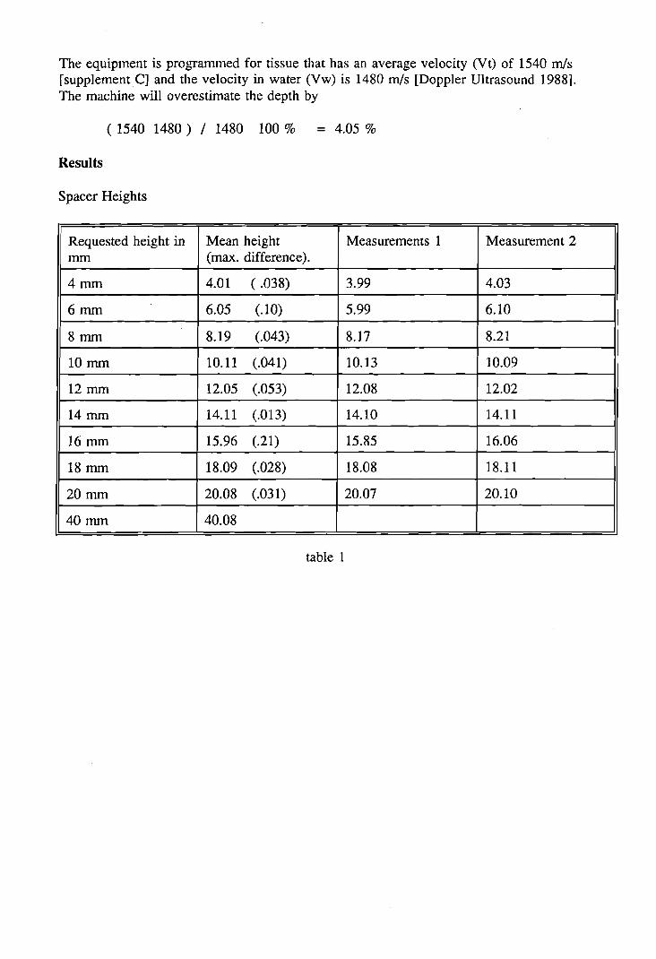
The equipment is programmed for tissue that has an average velocity (Vt) of 1540 m/s[supplementC] and the velocity in water (Vw) is 1480 m/s [Doppler Ultrasound 1988].The machine will overestimate the depth by

(1540 1480) / 1480 100 % = 4.05 %

Results

Spacer Heights

Requested height in Mean height Measurements 1 Measurement 2mm (max. difference).

4mm 4.01 ( .038) 3.99 4.03

6mm 6.05 (.10) 5.99 6.10

8mm 8.19 (.043) 8.17 8.21

lOmm 10.11 (.041) 10.13 10.09

12mm 12.05 (.053) 12.08 12.02

14 mm 14.11 (.013) 14.10 14.11

16 mm 15.96 (.21) 15.85 16.06

18 mm 18.09 (.028) 18.08 18.11

20mm 20.08 (.031) 20.07 20.10

40mm 40.08

table 1

Analyze results depth measurements

Twice a measurement set is created. In every measurment set there are 18 different depthmeasurements. Of each depth measurement there is done a duplicate. In figure 3 the 18means of the two measurement sets can be viewed.

Error in depth measurements

a

5040

- meas1 reala··· meas2 real

--•. _. measl car---B--- meas2 car

o

30

•••o

2010

1.8

1.6

1.4

1.2E 1.0Ec 0.8g 0.6w

0.4

0.2

0.0

-0.2

0

fig. 3:Error in depth measurement asfunction of the real depthaccording to the spacers. Thecorrected depth has acorrection for the difference insound velocity in water (1480m/s) and tissue (1540 m/s).

Depth in mm

Figure 4 contains a graph of the error in the height measurement of spacers using theultrasound system.

Error in height measurements 1- reg. line I

••

fig. 4:Error in height measurementof spacers

0.13

0.08

E0.03E

c~

e -0.02w• • •

•

•

•

••

•

-0.07 •

-0.12 •4 6 8 10 12 14 16 18 20 22

Height in mm

Characteristics of geometry measurements

Resolution

Hysteresis

Duplicity

:0.1 nun for depth until 30 nun. For measurements of more than 30 nun theresolution will be 0.2 mm.

:No hysteresis was observed in the measurements.

:within 0.1 nun till 30 nun and 0.2 mm for depth beyond 30 mm.

Reproducible :within 0.2 nun

Drift

Sensitivity

Linear

Stability

Accuracy

Conclusions

:No drift in zero point is observed during 8 hours.

:0.1 mm is in zoom mode 2 nun on screen.

:Depth scale is linear with the depth.

:Measurements did not show any instability

:Systematic error in depth is an over estimation of the depth about 4.6 %.The accidental error has standard deviation of 0.05mm.

Depth measurements are good reproducible and duplicable. The error in the measurementsseems to be proportional with the depth. The results are duplicable at 0.1 nun accurate andreproducible at 0.2 mm accurate.The measurement on the machine overestimate the real depth with 4.6 %. The velocity inwater is 4% lower then the average velocity in the human body. So the accuracy of theaveraged depth measurement is around 0.6 % of the depth. which is close to the 0.5 % inthe specifications.

Supplement E

Phantom and physiological measurements

1 Phantom measurements

1.1 Purpose

The string velocity of the phantom is very good reproducible. Also it is possible to givethe string a velocity pattern which is similar with blood flow patterns in the common carotid. Using this experiment, one can study the variation in the measurement of the velocityparameters on a constant subject.

1.2 Method

The string phantom exists of a string which moves through the water. The movement ofthe string is precisely (+/- 1 cm/s) known and the string velocity is measured with theultrasound machine in five different configurations. Twenty times the value of peakvelocity., mean velocity., time averaged (t.a.) peak velocity., end systolic. velocity., PIand RI are collected in each configuration which has a different measurement angle. Themeasurements are caried out automatically by the equipment.

•••

fig. 1: Measurement Configuration

1.3 Results

I Alpha II 66 1 62 158 1 50 IPeak 100 131-3.5 120-3.2 126-1.8 119-1.5

mean 100 67.5-2.6 96.5-4.6 94.5-3.5 100-1.5

peak sys. 116-5.8 115-4.3 115-8.2 109-3.9

end sys. 33.4-5.5 36.2-3.4 34.4-3.2 32.8-2.4

T.A. mean 20.7-1.1 27.5-1.8 27.8-1.0 26.2-0.84

T.A. peak 47.6-2.1 47.7-2.5 44.8-1.9 44.4-1.5

P.I. 2.73-0.38 2.73-0.38 2.76-0.40 2.81-0.28

R.I. 1.14-.039 1.14-.060 1.16-.033 1.15-.042

Table 1: Results of phantom measurements

The results are the mean and the standard deviation of 20 measurements. Those measurements were done in a row. These measurements are very good duplicable, but they arenot well reproducible especially the constant speed measurements..The measurement under66 degrees gave a lot of noise which probably influenced the measurements accuracy. Another problem gave the screen. When a video tape with the measurements is played then itis difficult to make distinction between the 3, 5, 6, 8, and 9.

~lpeakVel I t.a. mean I t.a. peakI PI I RI

Ivel. vel.

66 0.0495 0.0547 0.0437 0.140 0.0341

62 0.0371 0.0635 0.0524 0.140 0.0528

58 0.0712 0.0370 0.0426 0.146 0.0283

50 0.0357 0.0322 0.0331 0.100 0.0366

mean 0.0484 0.0469 0.0430 0.132 0.0379

Table 2: Relative Standard Variation1.4 Conclusions

The received Doppler signal is rather noisy resulting in a wide frequency band on thescreen. This broad band causes the peak velocity measurements to have a poor (error more25 %) accuracy. The mean velocity measurements are much better, but at times this isvery poor too. The string which is used consists of surgical silk. This silk wears out ratherquickly when it is used on the phantom. One problem is that the results of themeasurement can change during the wear process.The values best reproducible and accurate to the true value are mean velocity and the PI

and RI. Peak velocities showed too much variation. Still the measurement variation is toolarge for more detailed analysis. The phantom is too noisy maybe a different string willhelp. The noise is probably a result of the string source which reflects many coherentsignals.

2 Inter and i.,ntra subject variation measurements

2.1 Purpose

I would like to know the variation of diameter and velocity measurements within aindividual and is this variation similar between different individuals. This informationcould give an answer to the question how many measurements do I have to do to get agood result.

2.2 Method

Diameter

The diameter of the left common carotid is measured. On a longitudinal image thediameter is measured in the M-mode. Adjustments have been made to see the wallreflection lines as narrow as possible. The images have first been recorded on video tape.Measurements took place during replay in calculation mode. The measurement crosses areplaced just in the reflection line, moving away from the middle of the artery. The diameteris measured 5 times at more than 10 mm of the bifurcation.

Velocity

Also in the left common carotid the velocity is measured in the middle of the artery withtwo different sample volumes (SV 1 mm, and the averaged velocity over the whole arterySV 7.5 mm). The variation in the measurement is compared between the four individuals.Within the individual the velocity parameters have been measured 10 times in a row. Theangle correction on the machine is used.

2.3 Results

The results are summarized in the following tables (3,4). In every table the mean value isgiven and also the standard deviation

IMeasurement fif. I Minimum diameter Maximum diameter Diameter change

1 5.20-.00 5.68-.04 0.48-0.046

2 4.69-.05 5.50-.07 0.54-0.054

3 6.26-.05 6.80-.10 0.54-0.054

4 4.60-.07 5.35-.10 0.74-0.054

5 4.60-.00 5.02-.10 0.42-0.084

Table j: Diameter measurements III mm.

The next table contains velocity measurements in the left common carotid from fourdifferent healthy people. The participants were two man and two woman between 25 to65 years of age. Measurement A contains data collected with a small sample volume andB with a sample volume larger than the artery diameter ( SV is about 7.5 rom).

IMnr. II Peak sys. Imean vel. I t.a peale vel IPI I RI I1A 119-5.8 31.0-1.3 42.7-1.5 2.10-.10 .766-.011

B 118-6.6 33.0-1.9 43.2-1.7 2.20-.09 .794-.050

2A 113-5.3 23.8-.68 39.3-1.2 2.28-.18 .791-.026

B 96.7-3.9 24.8-1.5 34.9-1.2 2.29-.27 .819-.067

3A 100-3.17 28.0-.56 52.0-.84 1.28-.06 .864-.020

B 108-3.0 30.8-2.9 55.0-2.3 1.38-.09 .788-.080

4A 96.0-5.4 25.8-1.1 36.7-1.7 1.98-.21 .773-.050

B 89.0-4.3 23.8-1.0 33.6-1.6 2.07-.21 .783-.0316

Imean I 105-10.1% 27.6-13.1% 42.2-18.5% 1.95-20.2% 0.79-3.94%

Table 4: Velocity measurements

In table 5 the standard deviation is divided through the mean value. This makes it easierto compare the variation in the different measurement sets.

EJI peak sys. It.a. mean I tao peak vel. IPI IRIvel. vel.

1A 0.0488 0.0415 0.0362 0.0477 0.0146

1B 0.0556 0.0590 0.0385 0.0416 0.0623

2A 0.0471 0.0284 0.0306 0.0764 0.0323

2B 0.0399 0.0619 0.0345 0.1188 0.0821

3A 0.0317 0.0202 0.0163 0.0476 0.0233

3B 0.0279 0.0920 0.0410 0.0651 0.1013

4A 0.0559 0.0417 0.0455 0.1092 0.0646

4B 0.0483 0.0429 0.0483 0.1000 0.0404

I mean II 0.0444 10.0423 I0.0373 I0.0708 I 0.0514 ITable 5: Relative Standard Deviation

2.4 ConclusionDiameter measurements, including diameter changes, are good duplicable. Differencebetween inter and intra subject variation is clear. Measurements are possible with astandard variation of less then 0.1 mm.Velocity measurements showed more variation in both small and large sample volume.The measurements using the 1 mm sample volume show little less variation, all thoughdifferences are smalL Most reproduCible appears to be the peak velocity, t.a. meanvelocity, t.a. peak velocity and RI which have a inter subject variation of 5%. A part ofthe inter subject variation can be explained through a slight change of measurement angle.A one degree angle change gives at 60 degree 3% variation. The intra subject variability israther large in every parameter except the RI.

3 Inter and Intra Observer variation.

3.1 Purpose

Every observer will do the measurements a little different. In this experiment I study whatthe effects are of different probe positions on the results. I would like to find most suitableplace and position for velocity measurements.

3.2 Method

Of one healthy participant the velocity parameters are measured at two different positions.In every position the measurements are done ten times. The measurements are done in theleft common carotid. At each place the angle between the probe and vessel is varied between the different sets of measurements. The distance between transducer and carotidbifurcation (d) is measured with an accuracy of 5 mm. The angle alpha is measuredusing the features of the ultrasound machine which allow angle estimation with the highestaccuracy of 1 degree.

3.3 Results

Id - alpha II peak sys I t.lL mean I tao peak vel. IRI IPIIvel.. vel.

20-68 109-.99 22.6-.99 37.8-.97 2.39-.21 .825-.063

20-52 116-8.6 24.2-1.3 39.6-1.7 2.27-.15 .779-.013

40-70 139-6.9 23.2-1.2 43.9-1.6 2.56-.16 .817-.020

40-56 99.1-2.3 18.1-.79 28.6-2.2 2.83-.20 .824-.020

40-46 94.9-3.8 20.1-.84 29.7-2.7 2.64-.32 .845-.083

40-cross 46.3-3.1 11.1-.71 16.8-1.7 2.31-.19 .800-.018

I mean I 111*-15.7% 21.6*-11.5% 35.9*-18.3% 2.50-8.53% .815-2.80%

Table 6

The table 6 shows the average value of ten measurements with the standard deviation.The numbers with * are calculated without using the 40-cross measurement.

S peak mean mean peak PI RIvelocity. velocity.

20-68 0.0091 0.0438 0.0256 0.0885 0.0759

20-52 0.0747 0.0538 0.0427 0.0661 0.0165

40-70 0.0493 0.0525 0.0364 0.0621 0.0230

40-56 0.0234 0.0436 0.0767 0.0714 0.0237

40-46 0.0405 0.0420 0.0923 0.120 0.0985

40-cross 0.0660 0.0642 0.1035 0.0809 0.0228

I mean 11 0.0440 I 0.0500 I 0.0629 I 0.0816 I 0.0436 ITable 7: Relative standard deviation

Some remarks about the measurements:

20-68 Some peak velocities have been affected by PRF which was to low.40-46 To measure at this angle the you have to use some force which maybe influenced

the flow.

3.4 Conclusion

The results show a variation in the velocities values of more than 18% between thedifferent measurement position and orientation. From all the parameters the RI, PI andtime averaged mean velocity are the best reproducible. The variation within one set ofmeasurements is similar with the inter-intra subject measurement. Variation in ameasurement set is mostly about 6%. More practice will probably result in a betterreproduciblility of the measurements. From this experiment no clear conclusions can beextracted to locate the best position and angle.

Supplement F

Specifications of the Ultramark 9 HDI

Speci"fications

Physical Dimensions:

• Width: 27 inches• Height: 55 inches• Depth: 36 inches• Weight: 650 pounds (depends upon the hardcopy

device that is installed)

System Architecture:

• Digital beamformer• Modular microcomputer structure

Imaging Modes:

• Real-time 2D• M-mode• Doppler• Color 2D• Color M-mode

Operating Modes:

• 20• M-mode• Doppler• Color• Transducer Selection

• Setup• Calculations

Update Methods:

• Duplex• Auto Update• Simultaneous

Applications:

• Peripheral Vascular• Radiology• Cardiology• Obstetrical• Gynecological• Transcranial (pending scanhead availability)

• Fetal• Pediatric• Fertility

Specifications

Time Gain Compensation:

• Slidepot controls• 2DIM gain rotary control• Doppler gain rota!)' control• Color gain rotary control

Gray Shades:

• 64 in 20• 16 in M-mode• 256 in Doppler

Image Processing:

• Eight image processing curves• Dynamic contrast enhancement• Color scale enhancement• M-mode edge enhancement• Five Doppler grayscale curves

• Color maps

Scan Conversion:

• Sector for phased and curved array scanheads• Rectangular for linear array scanheads• 64 to 256 scan lines (scanhead dependent)

• Sector angle from 1 degree to 180 degrees

Image Memory:

• 64 normal resolution 2D images, 32 high resolution20 images. or 32 color images

• Expanded memory option provides 129 normal resolution 20 images, 64 high resolution 2D images, or64 color images

Frame Rate:

• Scanhead dependent

Operator Control System:

• Monitor brightness and contrast controls• Interactive touch-sensitive controls• Rotary controls• Slidepot controls

• Keyboard• Volume control• Footswitches• Color and tint controls for VCR playback

Digital Signal Processing:

• Selectable dynamic range

Specifications

• Automatic system bandwidth adjustment• Software-controlled bandwidth, filter, and frequency

adjustment

Image Modification:

• Zoom and pan of real-time or frozen 2D image• Up to eight times magnification of 2D images• Up to five times M-mode zoom• Color capture• Color persistence• Dynamic contrast enhancement

Progammability:

• Application presets• User-created presets• User-created color maps• User-created color scale enhancement m<>.ps• User-created OB analysis study that includes tables.

measurements, and graphs

• On-screen programming for internal and externalhardcopy devices

Display Annotation:

• Patient nanle and identification• Time and date• Biopsy guide lines• Automatic heart rate• Complete display annotation• Application-specific anatomic annotation• SPTAd and l\.1l values

Image Presentation:

• Up/down orientation• Left/right orientation• White-on-blackfblack-on-white

Scanheads:

• Linear Array, L5 38nml aperture• Linear Array, LlO-5 38mm aperture• Curved Array, C3 40R• Curved Array, C3.5 76R• Curved Array, C5 40R• Curved Array, C5 IVT• Phased Array, P3.5 28mm aperture• Phased Array, P7 8mm aperture

20:

• Image orientation marker• Image processing curves• Dynamic contrast enhancement• Dynamic range

• Color scale enhancement• 2D sector size and steering

M-mode:

• Sweep speeds: 25,50, and 100 mm/sec

• Edge enhancement

• Time markers• Color M-mode

• M-mode zoom

Doppler:

• Digital wall filters• Pulsed wave• Continuous wave• Adjustable sample volume (1.5 - 25 mm)• Adjustable zero baseline

• Normal or inverted display• Sweep speeds: 25, 50, and 100 mm/sec• Doppler gain control• High PRF with phased array• Doppler review• Multi-frequency capability·• Doppler processing curves• Low flow capability• Equivalent 5 MHz annotation in Vascular Analysis

Color:

• 2D Color• M-mode Color• User-created color maps• Color capture• Velocity, variance, and power displays• Dynamic motion differentiation• Color persistence

Measurements:

• 2D distance accuracy of 0.5 % of maximum distance• 2D circumference accuracy of 0.5 % of maximum

distance

• 2D area accuracy of 1.0 % of maximum area• M-mode distance accuracy of 0.5 % of maximum dis

tance

• M-mode differential time accuracy of + .02 to 2seconds depending on sweep speed

• M-mode s'lope accuracy of 0.5 %• Doppler angle accuracy of 1 degree• Doppler flow velocity accuracy of .01 % of maxi

mum velocity• Fetal age accuracy of 1 %

• Ejection fraction accuracy of 0.5 %

Analysis:

• Obstetrical• Gynecological

• Fertility• Cardiology• Cardiac Doppler

• Vascular• Radiology

Image Storage and Retrieval:

• Cineloop® Image Review• Dual Cineloop Image Review

• 20 Save-Recall• Doppler Review• VCR Playback• Frame Grabber

Hardcopy Devices:

• Standard VHS Video Cassette Recorder (VCR)• Super VHS VCR• Multi-Image camera• Color page printer• Black-and-white page printer• Report printer

Physiological Inputs:

• ECG- AMII standard ECG interface with UL-544

approved isolation- AMII standard ECG interface with UL-544

approved isolation- Bandwidth, 0.1 - 40 Hz

• Pulse- Bandwidth, 0.5 - 100 Hz

• Phono- Bandwidth, 0.5 - 500 Hz

~peClTIcations

- Bandpass filter response:25 - 560 Hz130 - 600 Hz180 - 600 Hz230 - 620 Hz

External VCR Interface:

• Composite video out (NTSC or PAL)• Luminance out «NTSC or PAL)• Chrominance out (NTSC or PAL)• Composite video in (NTSC or PAL)• Luminance in (NTSC or PAL)• Chrominance in (NTSC or PAL)

• Audio Channell out• Audio Channell in• Audio Channel 2 out• Audio Channel 2 in

External Monitor Interface:

• Red• Green (with Sync)

• Blue• Sync

External Report Printer Interface:

• Serial interface

Electrical Parameters:

• Power:- 100Vac, @ 47 to 63 Hz, 15A- 120Vac, @ 47 to 63 Hz, l2A- 220Vac,@ 47 to 63 Hz, 8.5A- 240Vac, @ 47 to 63 Hz, 8.5A

• Video:- NTSC- PAL

Monitors:

• One 9" RGB color monitor• One 9" monochrome monitor

Languages:

• English• French

• German

Specifications

Storage:

• Unified cable management system• Ultrasonic gel bottle• Biopsy guides and needles• One video cassette• Three multifonnat film cassettes

• ECG lead pads• Small wipe box• Print film

Safety Requirements:

• Electromechanical safety standards met:- IEC 60 I-I, International Electrotechnical Com

mission, Safety of Medical Electrical Equipment;Class I, Type BF

- UL-544, Underwriters Laboratories Standards forMedical and Dental Equipment

- VDE 0750, Association of German Engineers,Regulations for Electromedical Equipment

- C22.2 No. 125-1984, Canadian StandardsAssociation, Standard for Electromedical Equipment, Risk Class 2G

• Agency approvals- Canadian Standards Association (CSA) pending- Underwriters Laboratories (UL) pending- West German Quality, Reliability and Safety Test-

.. ..ing Organization (TUV-Technischen Uberwa-chungs-Verein) pending.

Advanced Technology Laboratories reserves the right tochange specifications contained herein or discontinuemanufacture at any time without prior notice. Currentspecifications are supplied with each system purchasedor are available from your ATL representative.

a view in ultrasound : analysis of the atl ultramark 9 as ... filebmgt931.139 wfw report nr.93.125 a...

Documents