a virtual hypercube routing algorithm for wireless healthcare networks

Chinese Journal of ElectronicsVol.19, No.1, Jan. 2010

A Virtual Hypercube Routing Algorithm for

Wireless Healthcare Networks∗

HUO Hongwei1,2, SHEN Wei2, XU Youzhi2 and ZHANG Hongke1

(1.School of Electronic and Information Engineering, Beijing Jiaotong University, Beijing 100044, China)

(2.Data Communication, JTH, Jonkoping University, Sweden)

Abstract — The application scenarios of wireless sensor

networks for health care systems are very complex, which

require a new communication schemes that can dynami-

cally fulfill these requirements and achieve efficient data

transmission. It brings a big challenge to routing, access

control, data transmission, storage and processing. This

paper presents a novel routing scheme named Virtual hy-

percube routing (VHR), in which the routing selection and

maintenance rules are defined based on a logical hypercube

structure. It can highlight good performance in data trans-

fer rate and query efficiency. Based on this structure, the

routing for health care can be implemented efficiently. We

evaluate the performance of VHR using simulation under

home and public area care scenarios. The results show that

this scheme performs high data transfer rate, low latency

and low overhead for communication under both static and

dynamic scenarios.

Key words — Wireless sensor networks, Home health

care, Routing protocols, Virtual hypercube.

I. Introduction

With increasing cost of healthcare and growing population of

seniors, healthcare using wireless sensor networks is being consid-

ered as a key solution to both improving the quality of healthcare

and reducing the cost of public healthcare service. Wireless sensor

networks for health care systems being composed of heterogeneous

sensor nodes (over multitude sensor devices) will be pervasively dis-

tributed, carried by people, deployed at home and daily public en-

vironments, and dynamically networked.

Fig.1 depicts a typical application scenario of wireless sensor

networks for health care systems, which can be divided into four

parts: at home, in vehicle, in public area and on body. The at

home part is usually pre-constructed and deployed at home or hos-

pital, consists of several sensor nodes and a gateway. The in vehicle

part is partially pre-constructed usually deployed in a traffic tool or

on an ambulance, which also consists of several sensor nodes and a

gateway. The in public area part is usually deployed in public area,

consisting of several sensor nodes only. The on body part, which is

a collection of sensor nodes worn on patient’s or elder’s body, pro-

vides a set of personalized physiological data collection with several

body sensor nodes and a gateway. In wireless health care systems,

the four parts link together to constitute an entire network. When

the patient is at home, the body area sensors will work as a mobile

part of the pre-constructed nodes, forming a home care network.

Critical data and home environmental data will be collected and

reported to the Care Center through proper gateways. When the

patient is in the traffic tool or ambulance, body area nodes and

nodes in traffic partially pre-constructed will constitute a special

vehicular care network. When the patient is in a public area, the

body area sensors will work as a mobile part and join the separated

part, together forming a public care network. Public area environ-

mental data will be collected and reported to the Care Center via

the body gateway. In addition to important data transmissions from

the sensor networks to the health care center, a large amount of data

are stored at local storage, and sent according to queries from the

service center through the appropriate gateway.

Fig. 1. An example of WSN based healthcare applications

Based on the scenario above, we summarize several requirements

of routing protocols for WSN for health care applications: (1) A

scalable and flexible routing structure to join mobile nodes and pre-

constructed nodes easily; (2) A query and report scheme to support

gateway access equally; (3) A robust scheme to support high data

rate and limited delay to fulfill emergency medical requirements; (4)

An energy efficiency policy to prolong the lifetime of sensors.

These require a new communication scheme that can dynami-

cally fulfill these requirements and achieve efficient data transmis-

sion. Currently, there are already a number routing schemes trying

to resolve some flanks of these issues[2−4,11−13]. We eagerly hope

to find an all-around scheme to fulfill all scenarios mentioned above.

In this paper, we define a novel routing scheme named Virtual

∗Manuscript Received Mar. 2008; Accepted Apr. 2009. This work is a part of VINNOVA project and supported by the member of

“OLD @HOME”, Ericsson Network Technologies AB/Acreo AB, Sweden, and partly supported by the National Natural Science Foundation

of China (No.60802016), National 863 Project of China (No.2007AA01Z241), “973 Program” of China (No.2007CB307100) and the Ph.D.

Student Scientific Research Innovation Fund of Beijing Jiaotong University (No.48022).

A Virtual Hypercube Routing Algorithm for Wireless Healthcare Networks 139

hypercube routing (VHR), in which all the nodes can be organized

into specific positions of a hypercube. The routing selection and

maintenance rules are defined based on a hypercube: node forwards

messages only to the node on the hypercube logically as the next

hop, which maintains the shortest hops to the destination. Based

on this structure, the routing for all health care scenarios can be im-

plemented efficiently. It is also an approach to join overlay routing

with network layer routing in other ad hoc and sensor networks.

The rest of this paper is organized as follows. Section II dis-

cusses the related works. Section III gives some preliminaries and

notations. Section IV describes the virtual hypercube routing algo-

rithm. Section V presents the analytical model to derive the per-

formance of this scheme. Section VI shows the evaluation results.

We close this paper with some conclusions in Section VII.

II. Related Works

Currently, there are a series of survey papers in routing proto-

cols with different kinds of classification[9,10]. Routing protocols are

usually derived from ad hoc networks, e.g. AODV, DSR, DSDV etc;

they can achieve a high performance in normal data communication

between nodes, but lack of adaption with the high layer applications,

which may cost large waste of communication resources.

Few of routing schemes trying to resolve some flanks of data

transmission issues in heterogeneous nodes WSNs, e.g. Directed

diffusion (DD)[2] and modified DD as well as data aggregation

protocols[11] to raise the achieving data rate and energy efficiency

in WSNs. The mapping between contexts to the interests is not

clear and the flooding-based route schemes are not efficient enough.

GHT[3,4] employs DHT and location based routing to achieve dis-

tributed data storage in WSNs. However, these approaches either

employ overlay structure, such as DHT or Hypercube, to achieve

the service and context aware, or seek the 3rd-party’s assistant, e.g.

localization technology in GHT, or piggyback this accessorial infor-

mation on the normal routing packets. Most of them achieve the

decision based on local information to minimize the communication

cost, which may increase complexity of the whole system.

Part of our inspiration in this paper is from VRR[6], which pro-

poses a novel scheme to implement P2P routing as well as DHT

functionality directly on the link layer. It achieves this by build-

ing a mixed routing table which joins the ring based DHT logical

neighbor status and physical neighbor status. However, in WSN

for health care systems, more queries will be in large scale WSN at

the same time and it is easy to imagine that ring-based structure

can’t achieve efficient routing with at most one backup path. In this

paper, we use hypercube instead of ring to organize sensor nodes,

which can highlight good performance[12,13].

There have been some recent works on joint Hypercube with

routing and related area. Blue Cube[14] is a hypercube establish-

ment approach in Bluetooth networks. ECube[5] proposes a scheme

to achieve efficient data filter, index and match for service awareness

routing and publish/subscribe communication. HTMRP[16] is fo-

cused on efficient multicast by use of hypercube structure. All these

approaches employ hypercube as an overlay structure. Hypercube is

also a well-known over layer structure and has been widely used in

context based search in the Internet community. Authors in Ref.[7]

propose a keyword search scheme with attributes using DHT-based

structure in P2P overlay networks; hypercube structure is used to

store keys with correlation attributes in neighbor nodes of a hyper-

cube. We believe that this overlay structure can also play a key role

in organizing sensor nodes and drive the routing directly based on

the lower layer (e.g. MAC layer). However, the complete hyper-

cube structure in these papers calls for a fixed number of nodes to

constitute a complete hypercube, which does not fit in the applica-

tion of sensor networks. In our approach, a concept of incomplete

hypercube is proposed to adjust hypercube being compatible with

sensor networks, which will be explained in Section III.

III. Preliminaries

1. Hypercube

Definition 1 b-Dimensional complete hypercube (b-DCH) is

a graph CHb(V, E), where V is the set of vertices and E is the set of

edges. Fig.2 shows an example of a 4-DCH. Each sensor node SNu

at the vertex u in V is represented by a unique b binary string, we

use SNu[q], 0 ≤ q ≤ b− 1, to denote the qth bit and qth dimension

of SNu, from right to left. For each pair of nodes SNu and SNv ,

we denote an edge (SNu, SNv), if and only if the harming distances

between the two sensors nodes is 1. The harming distance is defined

as

H(SNu, SNv) =∑b−1

q=0SNu[q]⊕ SNv [q]

where ⊕ denotes bitwise exclusive OR operation.

Definition 2 If ‖V ‖ < 2b and ‖E‖ < b2b−1, CHb(V, E) can

be defined as b-Dimensional incomplete hypercube (b-DIH). Where

‖ • ‖ represents the number of the vertices or the edges. Given a

pair of nodes SNu and SNv in b-DIH and the hamming distance p,

we can find at most p shortest disjoint paths with length p.

Fig. 2. 4 -Dimensional complete hypercube (4-DCH)

2. Addressing

In this section, we briefly introduce a simple addressing scheme

for health care system. As WSNs for health care system should be

deployed with some specific monitoring missions, individual sensor

should play a specific role by achieving some functional objectives.

We explain this scheme based on an example as illustrated in Fig.3.

We define 4 different objects (object 1 to object 4) and deploy 5

sensors (sensor1 to sensor 5) to achieve these objects in a hospital.

Object 1 can be achieved based on the data from sensors 1, 2 and 3.

On the contrary, sensor 1 should fulfill 4 objects in the WSNs. If we

define an addressing space expanded by all n objects of a network,

totally 2n, if the number of sensors less than 2n, all sensors can get

an address by its role to fulfill these objects, e.g. sensor 1 will get

the address 1111 according to the objects it should fulfill. It is also

common to meet the scenario that more than one sensor fulfill the

same objects at the same time in many applications. In this sce-

nario, we can split this object into several sub-objects to expend the

addressing space to make sure each node can get a unique address.

Fig. 3. An example of addressing scheme

140 Chinese Journal of Electronics 2010

IV. Framwork of Virtual HypercubeRouting

1. Proactive routing table

VHR uses b binary integers to identify nodes. Thus, the total

number of nodes in WSNs should be at most 2b. With this as-

sumption, all the nodes can be organized into specific positions of a

b-DIH.

In VHR, a node SNi, maintains a set of physical neighbors,

p Ni, which records the neighbors that can communicate with SNi.

The members of p Ni are decided by the link quality. Like most of

the routing protocols, we employ low layer protocol to estimate the

link quality. In our approach, each node broadcasts a Hello mes-

sage periodically. SNi only adds these nodes, from which the Hello

received ratio is higher than a specific threshold (e.g. 90 %), to its

p Ni. Any node in the VHR, SNi, also maintains a set of virtual

neighbors named virtual neighbor set, denoted as v Ni, the v Ni

members are the 1-hop hypercube neighbors of SNi.

However, the existence of a node’s 1-hop hypercube neighbors

cannot be guaranteed in practice. In this scenario, a set of comple-

mentary virtual neighbors, named complementary virtual neighbor

set, denoted as cv Ni. The nodes with shortest logical hops in the

hypercube will be added into the cv Ni. And cv Ni play the same

role as v Ni. The existence of a node in cv Ni or in v Ni is mutually

exclusive.

As both the identifiers of sensor nodes and the physical locations

are distributed randomly and independently, the v Ni members of

node SNi will be also randomly distributed across the whole net-

works.

Fig.4 shows an example of 4-DIH and its physical topology. In

this example, 13 sensor nodes are in the specific positions of a hy-

percube, as shown in Fig.4(a). The physical deployment of these

sensors in a specific area is shown in Fig.4(b), where three grey

nodes (1001, 1100, 0000) are the v N1000 members of the black one

(1000).

Fig. 4. An example of 4-DIH and its physical deployment

topology

Each node maintains a routing table. A normal routing ta-

ble entry include 5 key items: the destination which is a virtual

neighbor identifier or physical neighbor identifier (noted Dest.), the

physical neighbor to this destination (noted P Nei.), the physical

hops to the destination node (P Hop), updated identifier of this

path (Path ID) and the flag of the entry type (Type). The path ID

here is the sequence number of the latest packet to the Dest. During

the establishment procedure of the routing table, some packets to

search the route to other destinations may pass current node. This

information is also stored in the routing table as the complemen-

tary entry with the same structure as normal routing table items

but denoted by different type flag. Fig.5 illustrates an example of

the routing table of node 1000 shown in Fig.4. The first 4 entries

are the information about its physical neighbors. The 5th to the

7th entries in the table of Fig.5 are virtual neighbors. The first 7

entries are all the normal entries and flagged by N and the last 5

entries are the complementary entry and flagged by C.

2. New node initiation

When a new node, denoted as SNj , is initiated, it will also

broadcast Hello periodically. As mentioned above, any node should

listen to the Hello message and run Algorithm 1 below if it receives

a Hello message.

Type Dest. P Nei. P Hop Path ID

N 1011 1011 1 16

N 0101 0101 1 4F

N 0010 0010 1 3E

N 0011 0011 1 FF

N 0000 0101 2 6F

N 1100 0010 3 01

N 1001 0011 3 37

C 1110 1011 2 44

C 1111 0101 2 12

C 0001 0101 3 45

C 0100 0011 2 36

C 0111 1011 3 2F

Fig. 5. An example of the routing table at SN1000 (RT1000)

When new physical neighbors are found, the newly joined node

SNj will send a Table Setup message to its own identifier by this

physical neighbor. A Table Setup message includes the packet type,

RQ ID, the Origination Identifier, Destination Identifier, source

identifier, hops and RDR. RQ ID is a unique ID together with

the destination identifier to identify a table setup. The Origination

Identifier is the identifier who initiates the Routing Setup packet.

The Destination Identifier is the identifier of the destination of this

Routing Setup and the source identifier is the address of the node

who forwards this packet. The hops will be accumulated by 1 each

physical hop. The Route delay request (RDR) is the maximum

delay allowed for the current routing.

To support special applications in health care systems, SNi

distinguishes two different service scenarios, urgent-service scenario

and normal-service scenario. In our approach, SNi judges the com-

munication scenario in a greedy way by comparing the RDR with

local Hello delay (average between 2 neighbors). If the RDR/2b+1

higher than hello delay, it is normal-service. Otherwise, it is urgent-

service scenario.

Algorithm 1//node SNi, Set Timer=Constant1, Counter=Constant2while (received Hello from SNj) {

counter++;Timer–;call listen start();

}if (Timer expired && counter>= Constant 2){

listen stop();Counter=0;SNj → p Ni;call listen start();

}

Any node, e.g. SNi, which receives the Table Setup, will for-

ward this message using Algorithm 1, until one virtual neighbor of

SNj receives this message, or it’s failed to reach any virtual neigh-

bor.

Algorithm 2//node SNi, received Table Setup from SNj

Recev [id]= Table Setup;if (Recev [id]. Origination Identifier ==p Ni. *){//received Table Setup generated by its p neighbor

generate (RT [id]); // generate new RTi itemRT [id].P hop=FF;//disable current item in RTi

Recev [id]. Origination Identifier= SNi;//change Origination Identifier as itselfRecev [id]. hop++;


call generate(Routing Setup Confirm [Recev [id]. RQ ID]);all item in RTi++;

}else {

for (j = 1; j <=all item in RTi;j++){if (H(Recev [id]. Origination Identifier, SNi) < H(Recev [id].

Origination Identifier, RTi.[j]. Dest)){generate(RT [id]); //generate new RTi itemRTi. dest= Recev [id]. Origination Identifier;if (H(Recev [id]. Origination Identifier, SNi)== 1)//current node is the v neighbor of the Table Setup generator.{RTi.Type = N ;}else//current node, with minimum distance to Origination Identi-//fier, is not the v neighbor and p neighbor of the//Table Setup generator.{RTi. Type= C;}

RTi. p nei= Recev [id]. Source Identifier;RTi. path id= Recev [id]. RQ ID;call generate (Routing Setup Confirm [Recev [id]. RQ ID]);

all item in RTi++;}if (H(Recev [id]. Origination Identifier, SNi)== H(Recev [id].

Origination Identifier, RTi.[j]. Dest)){generate (RT [id]); //generate new RTi itemRTi. dest= Recev [id]. Origination Identifier;if (H(Recev [id]. Origination Identifier, SNi)== 1)//current node is the v neighbor of the Table Setup generator.{RTi. Type= N;}

else//current node, with minimum distance to Origination Identi-//fier, is not the v neighbor and p neighbor of the//Table Setup generator.{RTi. Type= C;}

RTi. p nei= Recev [id]. Source Identifier;RTi. path id= Recev [id]. RQ ID;call generate(Routing Setup Confirm [Recev [id]. RQ ID]);all item in RTi++;Recev [id]. Source Identifier= SNi;//change Origination Identifier as itselfRecev [id]. hop++;call forward(Routing Setup[Recev [id]. RQ ID]);

}if (H(Recev [id]. Origination Identifier, SNi)> H(Recev [id].

Origination Identifier, RTi.[j])){while(H(Recev [id]. Origination Identifier, RTi.[j]. Dest)==

minimum harming distance in RTi(RTi. Dest, Recev [id].Origination Identifier)) {//minimum harming distance in RTi(id) is the function to calcu-//late the minimum harming distance between all RTi. Dest//items and id

Recev [id]. Source Identifier= SNi;//change Origination Identifier as itselfRecev [id].hop++;call forward(Routing Setup[Recev [id]. RQ ID]);

}}}

Once the Table Setup message is stored as a normal or comple-

mentary item, then a Table Setup Confirm will be issued by the

virtual neighbor, SNi, and routed back through the reverse path to

SNj . In the Table Setup Confirm, the destination identifier will

be the origination identifier of Table Setup, SNj , the origination

identifier will be SNi, the destination of Table Setup and the RQ ID

will be the same as the Table Setup. When the physical neigh-

bor of the newly joind node received the Table Setup Confirm,

it will enable the entry whose Dest is SNj by setting P Hop as 1

and forward this Table Setup Confirm to SNj . On receiving a

Table Setup Confirm with destination to itself, SNj will add the

information in this packet as a normal entry in its routing table.

3. Routing discovery in normal scenario

If a VHR node SNi needs to send message to a specific node

SNj , SNi will check the routing table RTi if SNj is in RTi. If SNj

is an entry of RTi the message will be forwarded to SNj directly. If

no matching item, SNi will choose the entries holding the smallest

results and save them in a forwarding set of the specific destination

additionally with a RQ ID. We note a forwarding set from SNi to

SNj in SNi as FSij . The number of the entry in FSij is denoted as

|FSij |. The structure of FSij includes 〈RQ ID 1: RQ ID 2〉, source

identifier, Dest, p Nei, p Hop, path ID, RDR, and valid flag, where

a valid flag item identifies the availability of the entry. Initially, the

RDR, for each entry will be calculated by upper layer and stored in

FSij . Then SNi will initiate a Routing Request packet to search

the destination. The structure of Routing Request is the same as

Table Setup. The procedure of processing Routing Request will

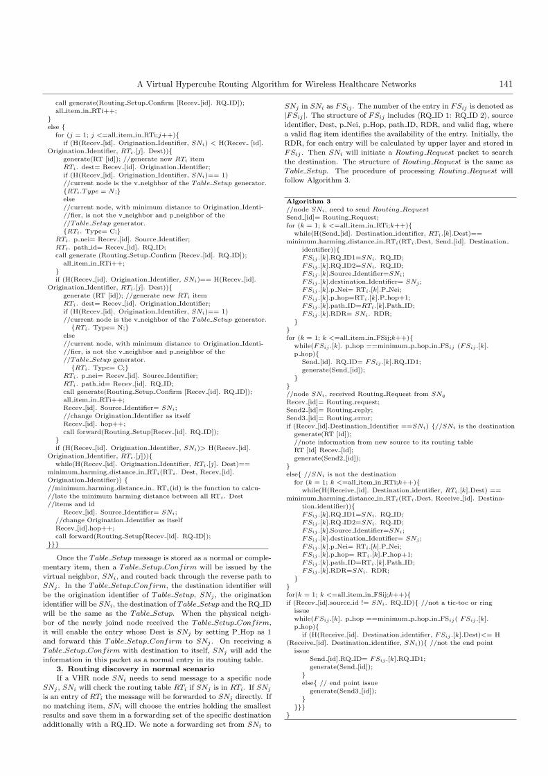
follow Algorithm 3.

Algorithm 3//node SNi, need to send Routing RequestSend [id]= Routing Request;for (k = 1; k <=all item in RTi;k++){

while(H(Send [id]. Destination identifier, RTi.[k].Dest)==minimum harming distance in RTi(RTi.Dest, Send [id]. Destination

identifier)){FSij .[k].RQ ID1=SNi. RQ ID;FSij .[k].RQ ID2=SNi. RQ ID;FSij .[k].Source Identifier=SNi;FSij .[k].destination Identifier= SNj ;FSij .[k].p Nei= RTi.[k].P Nei;FSij .[k].p hop=RTi.[k].P hop+1;FSij .[k].path ID=RTi.[k].Path ID;FSij .[k].RDR= SNi. RDR;

}}for (k = 1; k <=all item in FSij;k++){

while(FSij .[k]. p hop ==minimum p hop in FSij (FSij .[k].p hop){

Send [id]. RQ ID= FSij .[k].RQ ID1;generate(Send [id]);

}}//node SNi, received Routing Request from SNq

Recev [id]= Routing request;Send2 [id]= Routing reply;Send3 [id]= Routing error;if (Recev [id].Destination Identifier ==SNi) {//SNi is the deatination

generate(RT [id]);//note information from new source to its routing tableRT [id] Recev [id];generate(Send2 [id]);

}else{ //SNi is not the destination

for (k = 1; k <=all item in RTi;k++){while(H(Receive [id]. Destination identifier, RTi.[k].Dest) ==

minimum harming distance in RTi(RTi.Dest, Receive [id]. Destina-tion identifier)){FSij .[k].RQ ID1=SNi. RQ ID;FSij .[k].RQ ID2=SNi. RQ ID;FSij .[k].Source Identifier=SNi;FSij .[k].destination Identifier= SNj ;FSij .[k].p Nei= RTi.[k].P Nei;FSij .[k].p hop= RTi.[k].P hop+1;FSij .[k].path ID=RTi.[k].Path ID;FSij .[k].RDR=SNi. RDR;

}}for(k = 1; k <=all item in FSij;k++){if (Recev [id].source id != SNi. RQ ID){ //not a tic-toc or ring

issuewhile(FSij .[k]. p hop ==minimum p hop in FSij( FSij .[k].p hop){

if (H(Receive [id]. Destination identifier, FSij .[k].Dest)<= H(Receive [id]. Destination identifier, SNi)){ //not the end point

issueSend [id].RQ ID= FSij .[k].RQ ID1;generate(Send [id]);

}else{ // end point issue

generate(Send3 [id]);}

}}}}


Once a Routing Request packet reaches the destination SNj ,

a Routing Reply with the same structure and contents of corre-

sponding Routing Request is generated by SNj and routed back

to SNi through the reverse path. Once SNi receives the first

Routing Reply within the duration of RDR, it starts to dispatch

data to the destination with the active entry of local FSij . The

other Routing Reply will be ignored.

Normally, the principles defined above can cover nearly all sce-

narios and achieve a high packet rate. As the random mapping

between the physical locations and logical relations, three rare but

possible scenarios will cause packet delivery failures. The first sce-

nario is named tic-toc problem. As shown in Fig.6(a), when SNi,

receives a Routing Request with destination SNj from its physi-

cal neighbor SNk, it will select the possible next hop in RTi and

generate the corresponding FSij . However, according to the calcu-

lation result, if only one available entry in FSij , the next hop to

SNs is SNk, the Routing Request will be always repeated tic-toc

between SNk and SNi according to the former principle. The sec-

ond scenario is the loop problem. We treat this issue as a special

end-point problem. As shown in Fig.5(c), if the node SNj receives

a Routing Request with destination SNs from its physical neighbor

SNk, it finds that the RQ ID (e.g.=0x1121) an existed RQ ID in

FSjs. The third scenario is named endpoint problem. As shown in

Fig.6(b), we suppose that SNp also meets the tic-toc problem, but

in this scenario none of the entries even in all the expanding FSpj

is available, then an unlimited waiting time occurs in SNp. SNp

becomes an endpoint.

Fig. 6. Examples about tic-toc, end-point and loop problem

We break the tic-toc by expanding the FSij . When SNi

finds that Routing Request will be forwarded back, it will select

new entries in its routing table with sub-shortest harming distance

between Dest and the destination identifier in Routing Request.

Then mark the former entry in FSij unavailable and forward the

Routing Request according to the expanding entry (or entries). We

break this waiting by using Routing Error message, including the

packet type, RQ ID, Origination Identifier, and Destination Iden-

tifier. When SNp meets the endpoints problem, it will generate

a Routing Error and forward it back to SNi. As soon as the

Routing Error packet is receives, SNi will mark all the related

entries which choose SNp as the P Nei in its FSkj unavailable. If

SNi also becomes an endpoint, it will generate a Routing Error

and forward it back to SNk. In this scenario, the Routing Error

will also be generated by SNj and forwarded back to SNk. As soon

as receiving this message, SNk will also consider that it meets a

tic-toc problem and tries to break it by expanding its forwarding

set as the first scenario.

4. Routing maintains

If the lower layer reports that a physical neighbor SNj of the

node SNq is failure, SNq will delete all the information related with

SNj in RTq . Unlike other protocols, we do not need to issue any

Teardown message to other nodes to diffuse the information of the

failure nodes immediately but just delete the information about the

failed node locally. That is because the identifier of the failure node

existing in the routing table mainly plays a role of logical forwarder,

the true existence or not will not affect the routing performance of

the others. The only scenario of SNq issuing a Teardown message

to announce the failure of SNj is that SNq receives a request to

the destination node SNj , which is its former physical neighbor but

failure currently, from a remote node SNk. A Teardown will be

sent back along the reverse path to the source SNi. The informa-

tion about SNk in the old path will be disabled by marking P Hop

as FF. Fig.7(a) illustrates this procedure as an example. When the

Teardown is received by any nodes, the latest routing Path ID of

SNj should be reserved locally in Routing tables even this entry is

disabled. It is necessary because if the former is not failure but move

to a new position in the same network, the confliction maybe caused

by both the Teardown and Table Setup. An example is shown in

Fig.7(b). If SNj moves from SNq to SNk, then according to a

Routing Request from SNi to SNj , SNj will generate a Teardown

to route back to SNi. The Routing Request from SNi will arrive

SNi via SNk, the confliction will occur. In our approach, nodes

only obey the operation of the message with the newest Packet ID.

We have not discussed the mobility scenario separately, because the

mobility is a process that fails on the view of some nodes and joins

on the view of other nodes at the same time.

Fig. 7. Examples about node failures and mobility

5. Emergency message routing

While in urgent-service scenario, SNi greedily forwards

Routing Request to each Dest in FSij by choosing the P Nei as

the next hop with different RQ ID according to each entry of FSij

individually. All Routing Reply within the duration of RDR will

be chosen to dispatch data.

V. Analytical Model

In this section, we present the analytical model to derive the

performance of our schemes. To make this model tractable and

reasonably, we assume that all nodes are fixed and uniformly dis-

tributed in the service area.

1. Complexity

According to the complexity estimation approach in Ref.[6], if

a node SNi maintains at most n paths to its virtual neighbors and

the average path length is p, the maximum size of the routing table

entries will be pn at each node, if we assume that the destination

nodes are selected randomly and uniformly, the hops that a ran-

dom node find a path to a random destination is O(2n/np). The

average path length in an n−DCH is O(n), while in an n−DIH,

it is O(log2 n)[15]. Thus, the hops that a random node finds a

path to a random destination is O(2n/n2) in an n − DCH and

O(2n/n(log2 n)) in an n−DIH.

2. Route Achievable rate

Suppose the density of the nodes (totally n nodes) in a given

area is ρ and the coverage area of a node in our model is C. The

final route achievable rate is the probability of finding a path from

its physical neighbor to the destinations. It is helpful to analysis

the route achievable rate of these routes which is not existed in pre-

constructed routing tables. It is easy to derive the probability of

finding an available physical neighbor, noted as pn, as follows.

pn = min{ρnC, 1} (1)


And the probability of finding an available path

from a source to the destination is

pN =∑D

i=1Cikpi

n(1− pn)D−i (2)

where D is the number of destination nodes.

And in the emergency scenario, the proba-

bility of finding an available path from a source to

the destination is

pE =∑k

j=1Cjkpj

n(1− pn)k−j (3)

where k is the dimension of the hypercube.

3. End-to-end delay

As end-to end delay is an important perfor-

mance measure for emergency message, we only

model the delay for emergency scenario. As men-

tioned in Section V.1, if the average path length is

p, we can express the average delay for emergency

message as follows.

TD =1

p

p∑

l=1

(l

/(W − (

∑Nm=1gm)

n

2n

))(4)

where, W is the number of messages that a node

can process per second and gm is the mth node

which can generate emergency message and N is

the total number of these nodes.

VI. Evaluation

We use a self-defined simulation software

written in C++ language to compare the per-

formance of VRR[6] and VHR based on IEEE

802.15.4. We repeat each simulation 50 times.

Fig. 8. Streath of VRR and flooding

under static status

Fig. 10. The delay of VRR and VHR

under static and moving status

Fig. 9. The delivery rate of VRR and

VHR under static and moving

status

Fig. 11. The overhead of VRR and

VHR under static and moving

status

We first compare our schemes with flooding, which will always

find the shortest path between the source and the destination. We

compare VRR and flooding in 50 nodes and 100 nodes scenario. In

each scenario, we collect the data from a sink to all the other nodes

and count the average routing hops. Then we calculate the ratio of

hops in VHR to hops in flooding (which should be the shortest path)

in each scenario. The results are shown in Fig.8. From this result,

we can easily know that VRR achieve 30% of stretch than shortest

path in small scale networks and 60% of stretch than shortest path

in large scale networks.

The other metrics which we are interested in include delivery

rate (data finally achieve the destination in a protocol), average

end-to-end delay and the number of overhead per delivery under

the static status and 10% node moving status. In moving status,

the average mobility is 0-5m/s. The results are shown in Fig.9,

Fig.10 and Fig.11 individually. According to the result in Fig.9, we

know that both VHR and VRR can get a high achieve rate in small

scale networks. However, as our scheme does not contain any fail-

ure detection and auto recovery scheme, the delivery rate is a little

lower than VRR in large scale networks. From Fig.10, we know that

the delay of VHR is shorter than VRR in large scale networks. We

believe the reason is that VHR can provide high search efficiency as

an exponential based routing selection scheme than VRR. In Fig.11,

we can find that the overload is increasing with number of nodes,

but there is not a significant increase on the message per deliver in

VHR compared with VRR. VHR can achieve a short delay and sim-

ilar overload with VRR, as VHR is a hybrid routing protocol joint

both proactive and reactive schemes. We believe that the structure

of the hypercube brings good connectivity in both logical structure

and proactive routing tables, which can decrease the costs.

VII. Conclusion

This paper focus on the data transmission issues in wireless

sensor networks for health care systems. This scenario is very com-

plex, which requires a new scheme that can dynamically fulfill these

requirements and achieve efficient data transmission. It brings a

big challenge to routing, access control, data transmission, storage

and processing. This paper presents a novel routing scheme named

Virtual hypercube routing, in which the routing selection and main-

tenance rules are defined based on a logical hypercube structure. It

highlights good performance in delivery rate and query efficiency.

Based on this structure, the routing for health care can be imple-

mented efficiently. We evaluate the performance of VHR using sim-

ulation under the home care scenario and public area care scenario.

The results show that this scheme performs delivery rate, low la-

tency and low overhead under both static and dynamic status.

References

[1] E. Monton, J.F. Hernandez, J.M. Blasco, T. Herve, J. Mi-

callef, I. Grech, A. Brincat and V. Traver, “Body area network

for wireless patient monitoring”, IET Communications, Vol.2,

No.2, pp.215–222, 2008.

[2] C. Intanagonwiwat, R. Govindan, D. Estrin, J. Heidemann and

F. Silva, “Directed diffusion for wireless sensor networking”,

IEEE/ACM Transactions on Networking, Vol.11, No.1, pp.2–

16, 2003.

[3] S. Ratnasamy, B. Karp, L. Yin, F. Yu, D. Estrin, R. Govindan

and S. S, “GHT: A geographic hash table for data-centric stor-

age”, In Proceedings of First ACM International Workshop on

Wireless Sensor Networks and Applications (WSNA02), pp.78–

87, Sept. 2002.

[4] S. Ratnasamy, B. Karp, S. Shenker, Deborah Estrin and Li Yin,

“Data-centric storage in sensor nets with GHT, a geographic


hash table”, Mobile Networks and Applications, Vol.8, No.4,

pp.427–442, Aug. 2003.

[5] Eiko Yoneki and Jean Bacon, “eCube: Hypercube event for

efficient filtering in content-based routing”, International Con-

ference on Grid computing, High-performance and Distributed

Applications (GADA OTM 2007), LNCS 4804, pp.1244–1263,

Nov. 2007.

[6] M. Caesar, M. Castro, E. Nightingale, G. O’Shea and A.

Rowstron, “Virtual ring routing: Network routing inspired by

DHTs”, In Proceedings of the 2006 Conference on Applications,

Technologies, Architectures, and Protocols for Computer Com-

munications (Sigcomm 2006), pp.351–362, Sept. 2006.

[7] Yuhjzer Joung Liwei Yang and Chientse Fang, “Keyword search

in DHT-based peer-to-peer networks”, IEEE Journal on Se-

lected Areas in Communications, Vol.25, No.1, pp.46–61, Jan.

2007.

[8] C. Perkins, E. Belding-Royer and S. Das, “Ad hoc on-demand

distance vector (AODV) routing”, IETF Request for Comments

3561 (RFC3561), IETF, July 2003.

[9] Jamal N. Al-Karaki and Ahmed E. Kama, “Routing techniques

in wireless sensor networks: A survey”, IEEE Wireless Com-

munications, Vol.11, No.6, pp.6–28, Dec. 2004.

[10] D. Niculescu, “Communication paradigms for sensor networks”,

IEEE Communications Magazine, Vol.43, No.3, pp.116–122,

Mar. 2005.

[11] Hong Luo, Yonghe Liu and S.K. Das, “Routing correlated data

in wireless sensor networks: A survey”, IEEE Network, Vol.21,

No.6, pp.40–47, Nov. 2007.

[12] S.L. Johnsson and C.T. Ho, “Optimum broadcasting and per-

sonalized communication in hypercubes”, IEEE Transactions

on Computers, Vol.38, No.9, pp.1249–1268, Sept. 1989.

[13] Mario Schlosser, Michael Sintek, Stefan Decker, and Wolfgang

Nejdl, “HyperCuP Hypercubes, ontologies and efficient search

on P2P networks”, In Proceedings of the International Work-

shop on Agents and P2P Computing (AP2PC 2002), LNCS

2530, pp.112–124, July 2002.

[14] C.T. Chang, C.Y. Chang and J.P. Sheu, “BlueCube: Con-

structing a hypercube parallel computing and communication

environment over Bluetooth radio systems”, Journal of Par-

allel and Distributed Computing, Vol.66, No.10, pp.1243–1258,

Oct. 2006.

[15] Howard P. Katseff, “Incomppete hypercube”, IEEE Transac-

tions on Computers, Vol.37, No.5, pp.604–607, May 1988.

[16] R. Manoharan and P. Thambidurai, “Hypercube based team

multicast routing protocol for mobile ad hoc networks”, In Pro-

ceedings of the 9th International Conference on Information

Technology, 2006 (ICIT’06), pp.60–63, Dec. 2006.

[17] Upkar Varshney, “A framework for supporting emergency mes-

sage in wireless patient monitoring”, Decision Support System,

Vol.45, No.4, pp.981–996, Apr. 2008.

HUO Hongwei was born in 1982.

He is a Ph.D. student in the National En-

gineering Laboratory for Next Generation

Internet Interconnection Devices at Beijing

Jiaotong University. His current research

interests include wireless sensor networks,

wireless health care networks. (Email:

[email protected])

SHEN Wei was born in 1986. He is a researcher in the

Data Communication, School of Engineering, Jonkoping University,

Sweden. His current research interest is wireless sensor networks.

(Email: [email protected])

XU Youzhi was born in 1944, grad-

uated from Jiaotong University, Xi’an,

China, in electrical engineering (EE). He

received academic degrees of Tech. Licen-

tiate in 1989, Ph.D. degree in 1991 and Do-

cent in 2000, all in EE from Linkoping Uni-

versity. He is a professor and director of the

Data Communication, School of Engineer-

ing, Jonkoping University, Sweden. His

research interests include video processing

and communication, wireless sensor-actuator networks, ad-hoc net-

works and a lot of master and bachelor courses.

ZHANG Hongke was born in Sept.,

1957. He is a professor and director

of the National Engineering Laboratory

for Next Generation Internet Interconnec-

tion Devices at Beijing Jiaotong University.

He is also Ph.D. supervisor, senior mem-

ber in China Institute of Communications,

member of Electronics System Engineer-

ing Committee, commissioner of Supervis-

ing Committee of College and University

Teaching in the field of telecommunication. He is also the Chief Sci-

entist of the National Basic Research (973) Program “Theory and

Architecture of Universal Network and Pervasive Services”. His re-

search interests include modern information network infrastructure,

network basic technology and IPv6 network.

a virtual hypercube routing algorithm for wireless healthcare networks

Documents