A Visual Interaction Framework forDimensionality Reduction Based Data Exploration

Marco CavalloIBM Research

mcavall@us.ibm.research

Çagatay DemiralpIBM Research

cagatay.demiralp@us.ibm.research

ABSTRACTDimensionality reduction is a common method for analyzingand visualizing high-dimensional data. However, reasoningdynamically about the results of a dimensionality reductionis difficult. Dimensionality-reduction algorithms use complexoptimizations to reduce the number of dimensions of a dataset,but these new dimensions often lack a clear relation to theinitial data dimensions, thus making them difficult to interpret.

Here we propose a visual interaction framework to improvedimensionality-reduction based exploratory data analysis.We introduce two interaction techniques, forward projectionand backward projection, for dynamically reasoning aboutdimensionally reduced data. We also contribute two visualiza-tion techniques, prolines and feasibility maps, to facilitate theeffective use of the proposed interactions.

We apply our framework to PCA and autoencoder-based di-mensionality reductions. Through data-exploration examples,we demonstrate how our visual interactions can improve theuse of dimensionality reduction in exploratory data analysis.

Author KeywordsDimensionality reduction; interaction; bidirectional binding;visual embedding; forward projection; backward projection;PCA; autoencoder; deep learning; proline; feasibilitymap; exploratory data analysis; what-if analysis; Praxis.

INTRODUCTIONDimensionality reduction (DR) is widely used for exploratorydata analysis (EDA)[57] of high-dimensional datasets. DRalgorithms automatically reduce the number of dimensionsin data while maximally preserving structures, typicallyquantified as similarities, correlations or distances amongdata points [58]. This makes visualization of the data possibleusing conventional spatial techniques. For instance, analystsgenerally use scatter plots to visualize the data after reducingthe number of dimensions to two, encoding the reduceddimensions in a two-dimensional position.

Permission to make digital or hard copies of all or part of this work for personal orclassroom use is granted without fee provided that copies are not made or distributedfor profit or commercial advantage and that copies bear this notice and the full citationon the first page. Copyrights for components of this work owned by others than theauthor(s) must be honored. Abstracting with credit is permitted. To copy otherwise, orrepublish, to post on servers or to redistribute to lists, requires prior specific permissionand/or a fee. Request permissions from permissions@acm.org.

CHI 2018, April 21–26, 2018, Montreal, QC, Canada

c© 2018 Copyright held by the owner/author(s). Publication rights licensed to ACM.ISBN 978-1-4503-5620-6/18/04. . . $15.00

DOI:https://doi.org/10.1145/3173574.3174209

input Dimensionalityreduction output

bObserve Modify

a

input Dimensionalityreduction output

aObserveModify

b

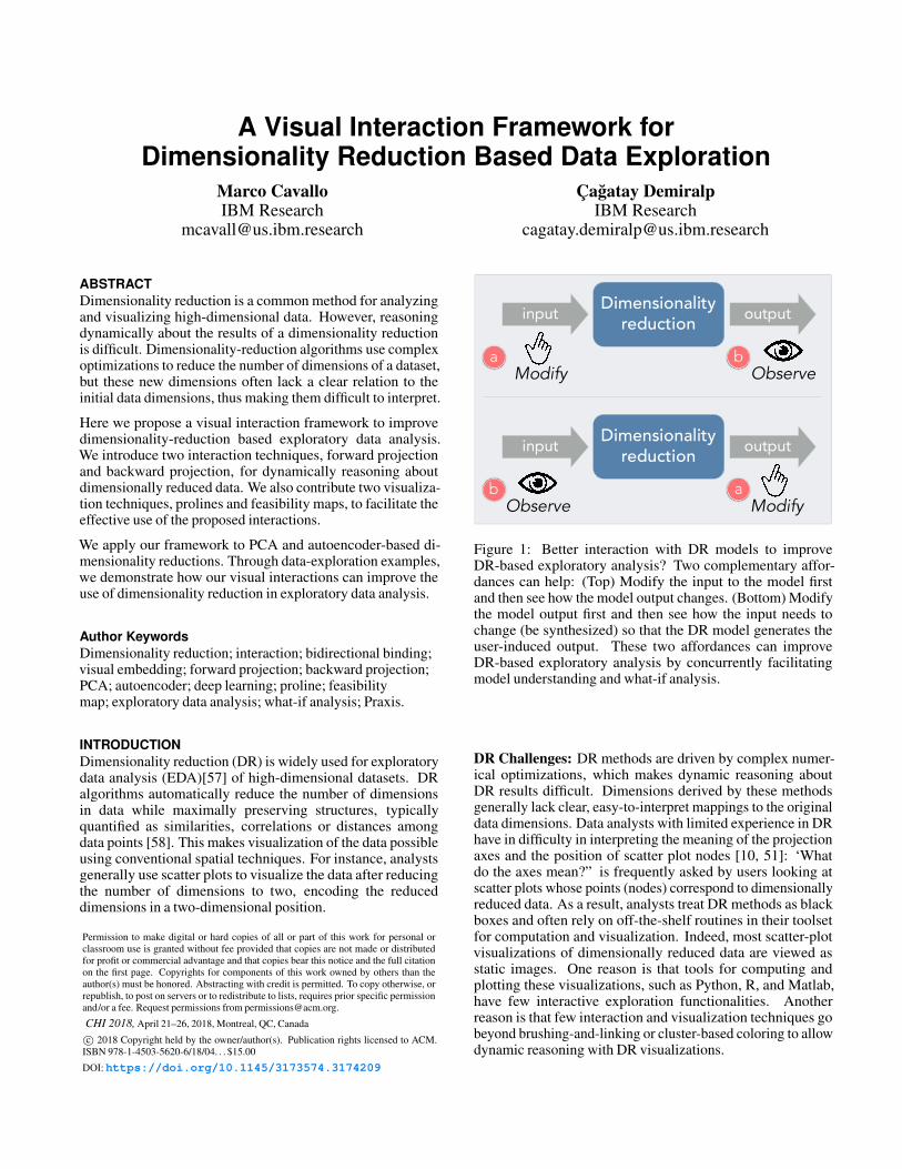
Figure 1: Better interaction with DR models to improveDR-based exploratory analysis? Two complementary affor-dances can help: (Top) Modify the input to the model firstand then see how the model output changes. (Bottom) Modifythe model output first and then see how the input needs tochange (be synthesized) so that the DR model generates theuser-induced output. These two affordances can improveDR-based exploratory analysis by concurrently facilitatingmodel understanding and what-if analysis.

DR Challenges: DR methods are driven by complex numer-ical optimizations, which makes dynamic reasoning aboutDR results difficult. Dimensions derived by these methodsgenerally lack clear, easy-to-interpret mappings to the originaldata dimensions. Data analysts with limited experience in DRhave in difficulty in interpreting the meaning of the projectionaxes and the position of scatter plot nodes [10, 51]: ‘Whatdo the axes mean?” is frequently asked by users looking atscatter plots whose points (nodes) correspond to dimensionallyreduced data. As a result, analysts treat DR methods as blackboxes and often rely on off-the-shelf routines in their toolsetfor computation and visualization. Indeed, most scatter-plotvisualizations of dimensionally reduced data are viewed asstatic images. One reason is that tools for computing andplotting these visualizations, such as Python, R, and Matlab,have few interactive exploration functionalities. Anotherreason is that few interaction and visualization techniques gobeyond brushing-and-linking or cluster-based coloring to allowdynamic reasoning with DR visualizations.

However, the ability not only to probe the results of a DRmodel but also actively to tinker with them is importantfor a model-based EDA, as experimentation is essential todata exploration [57]. Enabling an analyst to run variousinput and output scenarios and see how the underlying DRmodel—coupled with data—responds can facilitate modelunderstanding and is a prerequisite for what-if analysis.

Improving DR-Based Exploratory Analysis: In response,we propose a visual interaction framework to improveDR-based data exploration. To this end, we introduce two inter-action techniques, forward projection and backward projection,to help analysts dynamically explore and reason about scatterplot representations of dimensionally reduced data. We alsocontribute two visualization techniques, prolines and feasibilitymap, to facilitate the effective use of the proposed interactions.

The underlying idea (Figure 1) of our framework is that theability to induce change and observe the effects of that changeis essential for reasoning with DRs or any black-box models(more on this in Discussion). Forward projection enablesan analyst to interactively change data attributes input to aDR routine and observe the effects in the output. Backwardprojection complements forward projection by letting theanalyst make hypothetical changes to the output, the attributesof new dimensions, and observe which changes in the inputattribute values would produce the hypothesized changes inthe output. These affordances are useful for running what-ifscenarios as well as understanding the underlying DR process.

Contributions: Our high-level contribution is 1) a new frame-work that aims to enable users to dynamically change the inputand output of DRs and observe the effects of these changes.The design of the visual interactions that operationalize theunderlying purpose of the framework also has novel attributes.These contributions include 2) the forward projection inter-action using out-of-sample (OOS) extension, 3) the prolinevisualization along with its visual and interactive affordances,4) the backward projection interaction with interactive userconstraints, and 5) the feasibility map visualization.

Any DR algorithm with fast OOS extension (extrapolation) andinversion methods can be plugged in our framework. We applythe framework to PCA (principal component analysis) andautoencoder-based dimensionality reductions and demonstratehow it improves DR-based exploratory analysis.

Next we discuss related work and then introduce our frame-work interactions. We then present applications to PCA andautoencoder and give exploratory analysis examples, and thenelaborate on the scalability and accuracy of our methods. Thenwe discuss how the current model extends to black-box modelsat large, such as deep learning models, and how changes inmodel development practices can help improve explorabilityand interpretability of black-box models. We conclude bysummarizing our contributions and reflecting on the importanceof EDA tools that support interactive experimentation.

RELATED WORKOur work builds on prior research in direct manipulation andauxiliary visual encoding in scatter plots of dimensionalityreductions (DRs).

Direct Manipulation in DRDirect manipulation has a long history in human-computerinteraction [8, 31, 56] and visualization research (e.g. [52]). Di-rect manipulation techniques aim to improve user engagementby minimizing the perceived distance between the interactionsource and the target object [27].

Developing direct manipulation interactions to guide DRformation and modify the underlying data is a focus of priorresearch [11, 19, 23, 28, 29, 61]. For example, X/GGvis [11]supports changing the weights of dissimilarities input to theMDS stress function along with the coordinates of the embed-ded points in order to guide the projection process. Similarly,iPCA [28] enables users to interactively modify the weightsof data dimensions in computing projections. Endert et al. [20]apply similar ideas to additional dimensionality-reductionmethods while incorporating user feedback through spatialinteractions in which users can express their intent by draggingpoints in the plane.

Earlier work also uses direct manipulation to modify datathrough DR visualizations in order to support, e.g., exploratoryanalysis [28], multivariate network manipulation [59], explo-ration of trajectory clusters [50], movement trace analysis [16],and feature transformation [43]. Our work here aims tofacilitate DR-based exploratory analysis. Akin to forwardprojection and unconstrained backward projection techniques,iPCA [28] enables interactive forward and backward projec-tions for PCA-based DRs. However, iPCA recomputes fullPCAs for each forward and backward projection, and these cansuffer from jitter and scalability issues. Using out-of-sampleextrapolation [6, 58], our forward projection avoids re-runningdimensionality reduction algorithms. Unlike iPCA, we alsoenable users to interactively define constraints on featurevalues and perform constrained backward projection.

We refer readers to a recent survey [49] for an exhaustive dis-cussion of prior work on visual interaction with dimensionalityreduction.

Visualization in DR Scatter PlotsPrior work incorporates various visualizations in planar scatterplots of DRs in order to improve the user experience [3, 14, 18,22, 28, 38, 55]. Since low-dimensional projections are generallylossy representations of the high-dimensional data relations,it is useful to convey both overall and per-point dimensionality-reduction errors to users when desired. Researchers visualizederrors in DR scatter plots using Voronoi diagrams [3, 38] andcorrected (undistorted) the errors by adjusting the projectionlayout with respect to the examined point [14, 55].

Biplot was introduced [22] to visualize the magnitude and signof a data attribute’s contribution to the first two or three prin-cipal components as line vectors in PCA. Biplots are computedusing singular-value decomposition, regardless of the actualDR used, assuming the underlying DR is linear and the datamatrices needed to compute the decomposition are accessible.

Closest to our prolines are the enhanced biplots introduced byCoimbra et al. [15]. Enhanced biplots aim to extend biplots tononlinear DRs and assume only access to the projection func-tion of a DR, thus sharing similar assumptions and generaliza-

Modify data

Project

Select outputa

b

c

: change in data

: change in projection

: updated projection of modified data

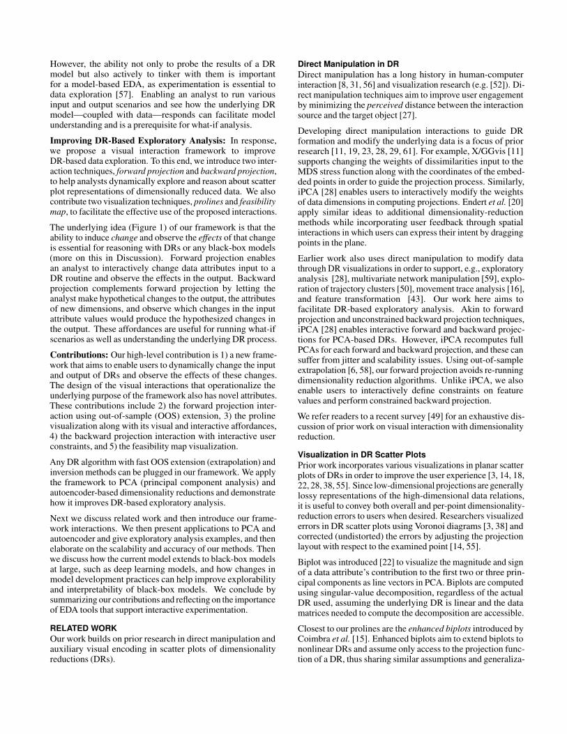
Forward Projection

Observe

x: input data point y: output projection of x

x’: input after user modification

y’: updated projection of the modified input x’

Figure 2: Forward projection enables users to: (a) select anydata point instance x that is input to a DR, (b) interactivelychange its high-dimensional feature values, and (c) observethe change ∆y in the point’s two-dimensional projection.

tion properties with prolines. Similarly to a proline construction,each axis of an enhanced biplot is constructed by connecting theprojections of points sampled on the range of the correspondingdata attribute. However, prolines differ from enhanced biplotsin a few aspects. Both enhanced and classical biplots visualizehow projections (reduced dimensions) change on average withchanging attribute values, whereas Prolines are computed foreach data and attribute and visualize projection changes locallyfor each data point. In this sense, prolines complement en-hanced biplots by constructing local axes of projection changewith respect to data attributes. To construct an attribute axis,enhanced biplots use values regularly sampled on the attribute’srange with a sampling rate uniform across axes, while keepingthe remaining attributes constant at their average values. On theother hand, we modulate the sampling rate with attribute vari-ances and decorate prolines with marks to communicate distri-butional characteristics of the underlying data point. More cru-cially, prolines differ from this earlier work in being interactivevisual signifiers that dynamically facilitate user interactions.

Stahnke et al. [55] use a grayscale map to visualize how a singleattribute value changes between data points in DR scatter plots.We introduce the feasibility map, a grayscale map, to visualizethe feasible regions in the constrained backward projectioninteraction.

We have presented our work at different stages of its develop-ment at two workshops. We introduced an initial version aspart of Clustrophile, an exploratory visual clustering analysistool [18]. We then presented our revised visual interactionsintegrated with Praxis, an interactive DR-based exploratoryanalysis tool, in a dedicated draft [12]. Here we give a unifiedtreatment of our work by formalizing it under a framework. Thecurrent work also demonstrates the use of our visual interactionsthrough several new data-exploration examples and provides anew discussion that relates the applicability of our framework toblack-box models, particularly deep learning models, at large.

VISUAL INTERACTIONSWe now discuss the interactions and the related visualizationsin our framework.

Forward ProjectionForward projection enables users to interactively changethe feature values of a data input x and observe how thesehypothesized changes in data modify the current projectedlocation y (Figure 2).

We compute forward projections using out-of-sample (OOS)extension (or extrapolation) [58]. OOS extension is theprojection of a new data point into an existing dimensionalityreduction (DR) using only the properties of the alreadycomputed DR. It is thus conceptually equivalent to testing atrained machine-learning model with data that was not partof the training set. Most common DR methods have OOSextension algorithms with desirable accuracy properties [6].

We propose using OOS extension as opposed to re-runningthe DR for two basic reasons. The first is scalability: OOScomputation is generally much faster than re-running thedimensionality reduction, and speed is critical in sustaining theinteractive experience. The second is preserving the constancyof scatter plot representations [5]. For example, re-running(training) a dimensionality-reduction algorithm with a newdata sample added can significantly alter the two-dimensionalscatter plot of the dimensionally reduced data, even though allthe original inter-datapoint similarities may remain unchanged.With OOS, forward projection animations change the positionof only the point attributes that the user interactively modifies.

Prolines: Visualizing Forward ProjectionsForward projection provides a scalable interaction to changethe attributes of a data instance and see how the dimensionalityreduction changes. We introduce prolines to let users seein advance what forward projection paths look like for eachdata point and feature. Through prolines, an analyst can seewhat directly start exploring data without considering forwardprojections exhaustively.

Prolines visualize forward projection paths using regularlysampled values for each feature and data point (Figures 3).Let xi be the value of the ith feature for the data point x. Wefirst compute the mean µi, standard deviation σi, minimummini and maximum maxi values for the feature in the datasetand devise a range I = [mini,maxi]. We then iterate over therange with step size cσi, compute the forward projections asdiscussed above, and then connect them as a path.

In addition to providing an advance snapshot of forwardprojections, a proline also conveys the relationship between thefeature distribution and the projection space. To that end, wedisplay along each proline a small light-blue circle indicatingthe position that the data point would assume if it had a featurevalue corresponding to the mean of its distribution; similarly,we display two small arrows indicating a variation of onestandard deviation (σi) from the mean (µi). The segmentidentified by the range [µi−σi,xi+σi] is highlighted andfurther divided into two segments. The green segment showsthe positions that the data point would assume if its featurevalue increased; the red one indicates a decreasing value. Thisenables users to infer the relationship between the feature spaceand the direction of change in the projection space.

Generating the proline for 𝒙𝑖

𝒙𝑖𝜇𝑖𝜇𝑖+𝜎𝑖 𝜇𝑖 − 𝜎𝑖

Increasing values

Decreasing values

𝜎𝑖𝜎𝑖

𝑚𝑖𝑛𝑖𝑚𝑎𝑥𝑖

A proline visually encodes distribution information

One proline is generated for each feature

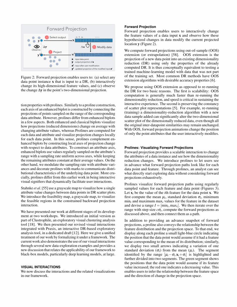
Figure 3: Proline construction. For a given dimension (feature)xi of a point x in a dataset, we construct a proline by connectingthe forward projections of data points regularly sampled froma range of x values, where all features are fixed but xi varies.A proline also encodes the forward projections for the xi valuesin [µi−σi,µi+σi] with thick green and red line segments,providing a basic directional statistical context. µi is themean of the ith dimension in the dataset, the green segmentrepresents forward projections for xi values in [xi,µi+σi], andthe red segment represents xi values in [µi−σi,xi].

Backward ProjectionBackward projection complements the forward projectioninteraction by enabling a user to interactively change outputattributes and observe how the input attributes change as theDR routine produces the user-induced output. Consider thefollowing scenario: a user looks at a projection and, seeinga cluster of points and a single point projected far from thisgroup, asks what changes in the feature values of the outlierpoint would bring it near the cluster. Now the user can playwith different dimensions using forward projection interactionsto move the current projection of the outlier point near thecluster. It would be more natural, however, to move the pointdirectly and observe the change.

Back or backward projection maps a low-dimensional datapoint back into the original high-dimensional data space. Forlinear DRs, back projection is typically done by applying theinverse of the learned linear DR mapping. For nonlinear DRs,earlier research proposed DR-specific backward-projectiontechniques. For example, iLAMP [2] introduces a back-projection method for LAMP [30] using local neighborhoodsand demonstrates its viability over synthetic datasets [2]. Re-searchers also investigated general backward-projection meth-

ModifyBack-project

Select outputa

b

c

: change in data

: change in projection

: updated data of modified projection

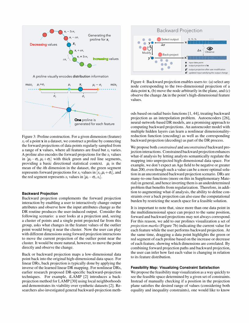
Backward Projection

Observe

x: input data point y: output projection of x

y’: output projection after user modification

x’: updated input satisfying the output change

Figure 4: Backward projection enables users to: (a) select anynode corresponding to the two-dimensional projection of adata point x, (b) move the node arbitrarily in the plane, and (c)observe the change ∆x in the point’s high-dimensional featurevalues.

ods based on radial basis functions [1, 44], treating backwardprojection as an interpolation problem. Autoencoders [26],neural-network-based DR models, are a promising approach tocomputing backward projections. An autoencoder model withmultiple hidden layers can learn a nonlinear dimensionality-reduction function (encoding) as well as the correspondingbackward projection (decoding) as part of the DR process.

We propose both constrained and unconstrained backward pro-jection interactions. Constrained backward projection enhanceswhat-if analysis by letting analysts semantically regulate themapping into unprojected high-dimensional data space. Forexample, we don’t expect an Age field to be negative or greaterthan 200, even though such a value can be a more optimal solu-tion in an unconstrained backward projection scenario. DRs aremany-to-one functions (more on this in Supplementary Mate-rial) in general, and hence inverting them is an underdeterminedproblem that benefits from regularization. Therefore, in addi-tion to augmenting what-if analysis, the ability to define con-straints over a back projection can also ease the computationalburden by restricting the search space for a feasible solution.

It is important to note that, since more than one data point inthe multidimensional space can project to the same position,forward and backward projections may not always correspond.For this reason, we add to our prolines visualization a set ofprojection marks (Figure 7b) indicating the current value foreach feature while the user performs backward projection. Atthe same time, dragging a data point highlights the green orred segment of each proline based on the increase or decreaseof each feature, showing which dimensions are correlated. Bycombining forward projection paths and backward projection,the user can infer how fast each value is changing in relationto its feature distribution.

Feasibility Map: Visualizing Constraint SatisfactionWe propose the feasibility map visualization as a way quickly tosee the feasible space determined by a given set of constraints.Instead of manually checking if a position in the projectionplane satisfies the desired range of values (considering bothequality and inequality constraints), one would like to know

Figure 5: Feasibility map. The feasibility map is constructed bysampling the projection plane through constrained backwardprojection and then verifying the existence of each solution(left). The darker area of the map, computed throughinterpolation, corresponds to the positions of the plane thatwould break the constraints for the specified data point (right).

in advance which regions of the plane correspond to admissiblesolutions. In this sense, a feasibility map is a conceptualgeneralization of prolines to the constrained backwardprojection interaction.

To generate a feasibility map, we sample the projection planeon a regular grid and evaluate the feasibility at each grid pointbased on the constraints imposed by the user, obtaining a binarymask over the projection plane. We render this binary mask overthe projection as an interpolated grayscale heatmap in whichdarker areas indicate infeasible planar regions (Figure 5). Withaccuracy determined by the grid resolution, the user can seewhich areas a data point can assume in the projection plane with-out breaking the constraints. In backward projection, if a datapoint is dragged to a position that does not satisfy a constraint,its color and the color of its corresponding projection marksturn to black. If the user drops the data point in an infeasibleposition, the point is automatically moved through animationback to the last feasible position to which it was dragged.

APPLICATIONSWe apply our framework to PCA (principal component anal-ysis) and autoencoder-based dimensionality reductions (DRs)and demonstrate how it improves DR-based exploratory analy-sis. We choose PCA and autoencoder because they respectivelycover linear and nonlinear DR cases and have effective exten-sion and inversion methods. PCA, among the most frequentlyused DR methods, is effective for rapid initial exploratory anal-ysis and requires no parameter tuning. Note that the frameworkcan be applied to any DR algorithm with fast inversion and out-of-sample (OOS) extension methods. As their fast inversionand extension methods become available, the framework caneasily applied to other popular DR methods such as t-SNE [41].

In what follows we first briefly introduce Praxis, a new toolfor interactive DR-based data analysis that integrates ourframework interactions, and then discuss applications throughexamples of exploration of tabular and image datasets.

Praxis: To demonstrate the use of our interaction andvisualization techniques, we integrate them in Praxis, an

interactive tool for DR-based exploratory analysis. Althoughdesign and implementation details of Praxis are out of thescope of this paper, we give a brief description to help thereader follow the rest of the paper.

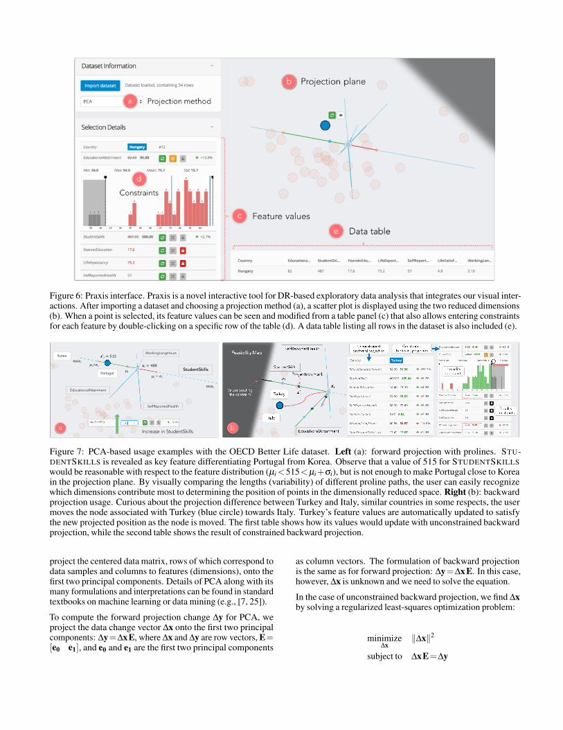
Praxis’ user interface has four basic elements: Data Import,Selection Details, Projection, and Data Table. Through theData Import panel (Figure 6a), users can import a dataset inCSV format, set the projection method (e.g., PCA) using adrop-down selection menu, and view the resulting dimensional-ity reduction as a scatter plot in the Projection plane (Figure 6b).As customary, Praxis uses the first two reduced dimensions(e.g., the first two principal components for PCA) as axes.

The results of forward and backward projection, along with thetwo visualizations prolines and feasibility map, are displayedin the Projection plane. The id (name) of a data point is shownon mouse hover, while clicking performs selection, showingits feature values in the Selection Details panel, a dedicatedsidebar(Figure 6c). The Selection Details panel is used toperform forward projections (clicking on a dimension makes itsvalue modifiable) and to inspect changes in feature values whenbackward projection is used. The three buttons next to the fea-ture column in this panel respectively 1) reset the feature to itsinitial value, 2) toggle the inequality constraints on the feature,and 3) lock the feature value to the current—modified—value(i.e., toggles the equality constraint).

Double-clicking the row associated with a feature displaysa histogram representing its distribution below the selectedrow, showing some basic statistics (Figure 6d). The currentvalue of the feature is represented by a blue line and a cyanline indicates the distribution mean. Bins of the histogram arecolored similarly to prolines: green for increasing values andred for decreasing values with respect to the original featurevalue. Users can set constraints on the feature through directmanipulation in the histogram visualization. Dragging oneof the two black handles lets the user set or unset lower andupper bounds for a feature distribution, thus defining a set ofconstraints for a specific data point.

Finally, selecting a data point in the Projection plane displaystwo buttons that respectively enable 1) resetting its featurevalues (and position) to their original value and 2) showing atooltip on top of its k currently nearest neighbors, in order tofacilitate reasoning about similarity with other data samples;this is particularly useful when performing back projection.

We integrate PCA and autoencoder as dimensionality-reductionmethods in Praxis. Next we discuss the first application of ourframework, PCA.

Application 1: PCAPrincipal component analysis (PCA) is one of the mostfrequently used linear dimensionality-reduction techniques.PCA computes (learns) a linear orthogonal transformationof the empirically centered data into a new coordinate framein which the axes represent maximal variability. The processis identical to fitting a high-dimensional ellipsoid to the data.The orthogonal axes of the new coordinate frame, which arealso the principal axes, are called principal components. Toreduce the number of dimensions to two, for example, we

b

Figure 6: Praxis interface. Praxis is a novel interactive tool for DR-based exploratory data analysis that integrates our visual inter-actions. After importing a dataset and choosing a projection method (a), a scatter plot is displayed using the two reduced dimensions(b). When a point is selected, its feature values can be seen and modified from a table panel (c) that also allows entering constraintsfor each feature by double-clicking on a specific row of the table (d). A data table listing all rows in the dataset is also included (e).

Portugal

𝒙𝑖 = 488

𝒙′𝑖 = 515

𝜇𝑖

𝜇𝑖+𝜎𝑖

𝜇𝑖 − 𝜎𝑖

𝑚𝑖𝑛𝑖

StudentSkills

SelfReportedHealth

EducationalAttainment

WorkingLongHours

Portugal

Korea

𝒙𝑖 = 488

𝒙′𝑖 = 515

𝜇𝑖

𝜇𝑖+𝜎𝑖

𝜇𝑖 − 𝜎𝑖

𝑚𝑎𝑥𝑖

𝑚𝑖𝑛𝑖

StudentSkills

SelfReportedHealth

EducationalAttainment

WorkingLongHours

Increase in StudentSkillsba

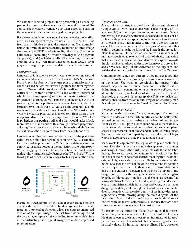
Figure 7: PCA-based usage examples with the OECD Better Life dataset. Left (a): forward projection with prolines. STU-DENTSKILLS is revealed as key feature differentiating Portugal from Korea. Observe that a value of 515 for STUDENTSKILLSwould be reasonable with respect to the feature distribution (µi<515<µi+σi), but is not enough to make Portugal close to Koreain the projection plane. By visually comparing the lengths (variability) of different proline paths, the user can easily recognizewhich dimensions contribute most to determining the position of points in the dimensionally reduced space. Right (b): backwardprojection usage. Curious about the projection difference between Turkey and Italy, similar countries in some respects, the usermoves the node associated with Turkey (blue circle) towards Italy. Turkey’s feature values are automatically updated to satisfythe new projected position as the node is moved. The first table shows how its values would update with unconstrained backwardprojection, while the second table shows the result of constrained backward projection.

project the centered data matrix, rows of which correspond todata samples and columns to features (dimensions), onto thefirst two principal components. Details of PCA along with itsmany formulations and interpretations can be found in standardtextbooks on machine learning or data mining (e.g., [7, 25]).

To compute the forward projection change ∆y for PCA, weproject the data change vector ∆x onto the first two principalcomponents: ∆y=∆xE, where ∆x and ∆y are row vectors, E=[e0 e1], and e0 and e1 are the first two principal components

as column vectors. The formulation of backward projectionis the same as for forward projection: ∆y=∆xE. In this case,however, ∆x is unknown and we need to solve the equation.

In the case of unconstrained backward projection, we find ∆xby solving a regularized least-squares optimization problem:

minimize∆x

‖∆x‖2

subject to ∆xE=∆y

We find a least-norm solution ∆x∗ by multiplying ∆y withthe pseudoinverse of E [9]. This is equivalent to setting∆x∗=∆yET as the pseudoinverse of a real-valued orthonormalmatrix is equal to the transpose of the matrix.

For constrained backward projection, we find ∆x∗ by solvingthe following quadratic optimization problem:

minimize∆x

‖∆xE−∆y‖2

subject to C∆x=dlb≤∆x≤ub

Here C is the design matrix of equality constraints, d is theconstant vector of equalities, and lb and ub are the vectors oflower and upper boundary constraints.

To better understand how these variables are determined,consider a dataset that contains the HEIGHT, WEIGHT,AGE and SCORE values for a set of people. Using the backprojection interaction, we would like to experiment with theprojection of an individual with the attribute values HEIGHT=174, WEIGHT=68,AGE=30, and SCORE=8.5. Suppose weconstrain AGE to stay fixed (an equality constraint), SCORE tobe between 8 and 10, HEIGHT and WEIGHT to be non-negative(inequality constraints) using the Praxis interface. Praxis wouldset lb = [−174,−68,−∞,−0.5] and ub = [+∞,+∞,+∞,1.5]for the inequality constraints. For the equality constraint onAGE, Praxis sets d=[0,0,30,0] and C to be a 4×4 matrix with[0,0,1,0] in its third row and zeros elsewhere.

We now discuss a data exploration facilitated by our visualinteractions in which the underlying dimensionality reductionmodel is PCA. Drawing on earlier work [55], we use the OECDBetter Life dataset that contains eight numerical socioeconomicdevelopment indices of 34 OECD member countries.

Example: OECD Better Life IndexZeynep is a data scientist working for a nonprofit organizationfocusing on economic development. She wants to use thedataset to understand the current situation of various countriesin the world and validate her own hypotheses. After importingthe dataset into Praxis and choosing PCA as the dimensionality-reduction method, Zeynep observes that the projection planecontains three clearly separated clusters: (1) a large set ofwesternized (mostly European) countries, (2) Portugal, Turkey,Mexico and Chile, and (3) Korea and Japan. Noticing thatPortugal is relatively distant from all other European countries,Zeynep wants to understand which development indicesdetermine its position (Figure 7a). She selects the data point andobserves how, of the eight generated prolines, only four of themare long enough to be visible—and they are associated (fromthe longest to the shortest) to the features STUDENTSKILLS,EDUCATIONALATTAINMENT, SELFREPORTEDHEALTH andWORKINGLONGHOURS. Immediately upon looking at theprolines, Zeynep understands that the remaining four develop-ment indices have almost no influence on the current projection,while STUDENTSKILLS (the longest proline) appears to bethe most relevant feature. To verify this, she tries to modifythe feature value of LIFESATISFACTION and observes that,no matter how large the change, the data point associated toPortugal does not move in the projection plane. On the other

hand, slightly changing the value of STUDENTSKILLS movesthe point quickly along the associated proline. By observingthe direction of each proline, Zeynep understands that featurescausing Portugal to be distant from the European cluster areEDUCATIONALATTAINMENT and SELFREPORTEDHEALTH,while STUDENTSKILLS seems to be the main feature differ-entiating it from Korea and Japan. Zeynep now wants to verifyif a reasonable increase in STUDENTSKILLS would makePortugal more similar to Korea. While observing the featuredistribution information on the associated proline, she seesthat Portugal would have to increase STUDENTSKILLS wellbeyond the maximum value of the distribution.

Zeynep then focuses on another outlier country that has stronghistorical ties to Europe but has never been part of it: Turkey(Figure 7b). She selects the data point associated to Turkey anddrags it towards one of the closest European countries, Italy.Feature values of Turkey are updated through (unconstrained)backward projection (Figure 7b, first table) and Zeyneprealizes that the country would have to increase almost all itsdevelopment indices to become more similar to Italy; onlythe WORKINGLONGHOURS would have to decrease. Whiledragging the data point, Zeynep observes from the color ofthe highlighted prolines that STUDENTSKILLS, SELFREPORT-EDHEALTH and EDUCATIONALATTAINMENT are positivelyintercorrelated (green color), while WORKINGLONGHOURSis negatively correlated (red). Zeynep, wanting to create amore realistic scenario, now assumes the Turkish governmentcannot directly control indices such as LIFEEXPECTANCY,SELFREPORTEDHEALTH and LIFESATISFACTION, andsets an equality constraint for these features. However, thegovernment can invest a certain amount of money in education,with the plan of increasing the STUDENTSKILLS index to 490over the next five years. Zeynep sets the inequality constrainton STUDENTSKILLS through a dedicated user interface(Figure 7b, second table). She directly observes from thefeasibility map how the region of the projection plane aroundItaly is reachable given the specified constraints. Then Zeynepagain moves Turkey towards Italy through backward projectionand observes how this time its feature values are updatedto respect the user-defined constraints (Figure 7b, secondtable). While dragging the point, Zeynep further validates herhypothesis by checking the changing position of projectionmarks that indicate the current value of each feature withrespect to the distribution information encoded on prolines.

Application 2: AutoencoderIn a second application, we demonstrate the frameworkinteractions on autoencoder-based DR. An autoencoder is an ar-tificial neural network model that can learn a low-dimensionalrepresentation (or encoding) of data in an unsupervisedfashion [48]. Autoencoders using multiple hidden layers withnonlinear activation functions can discover nonlinear mappingsbetween high-dimensional datasets and their low-dimensionalrepresentations. Unlike many other DR methods, an autoen-coder gives mappings in both directions between the dataand low-dimensional (latent) spaces [26], making it a naturalcandidate for application of the interactions introduced here.

We compute forward projection by performing an encodingpass on the trained autoencoder for a user-modified input. Tocompute backward projection, we perform a decoding pass onthe autoencoder for the user-changed output projection.

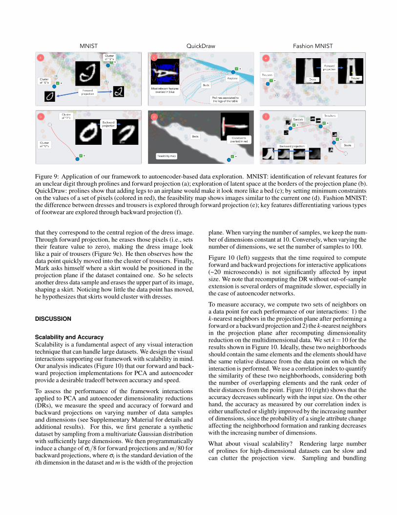
For the examples below, we trained an autoencoder model (Fig-ure 8) with six layers of respective sizes (128,32,2,32,128,784)from the first hidden layer to the output layer. Our examplesbelow are from the dimensionality reduction of three imagedatasets: (1) MNIST handwritten digit database, (2) GoogleQuickDraw (containing 50 million drawings in 345 differentcategories), and (3) Fashion MNIST (including images ofclothing articles). All three datasets contain 28x28 pixelgrayscale images, represented as data vectors of 784 features.

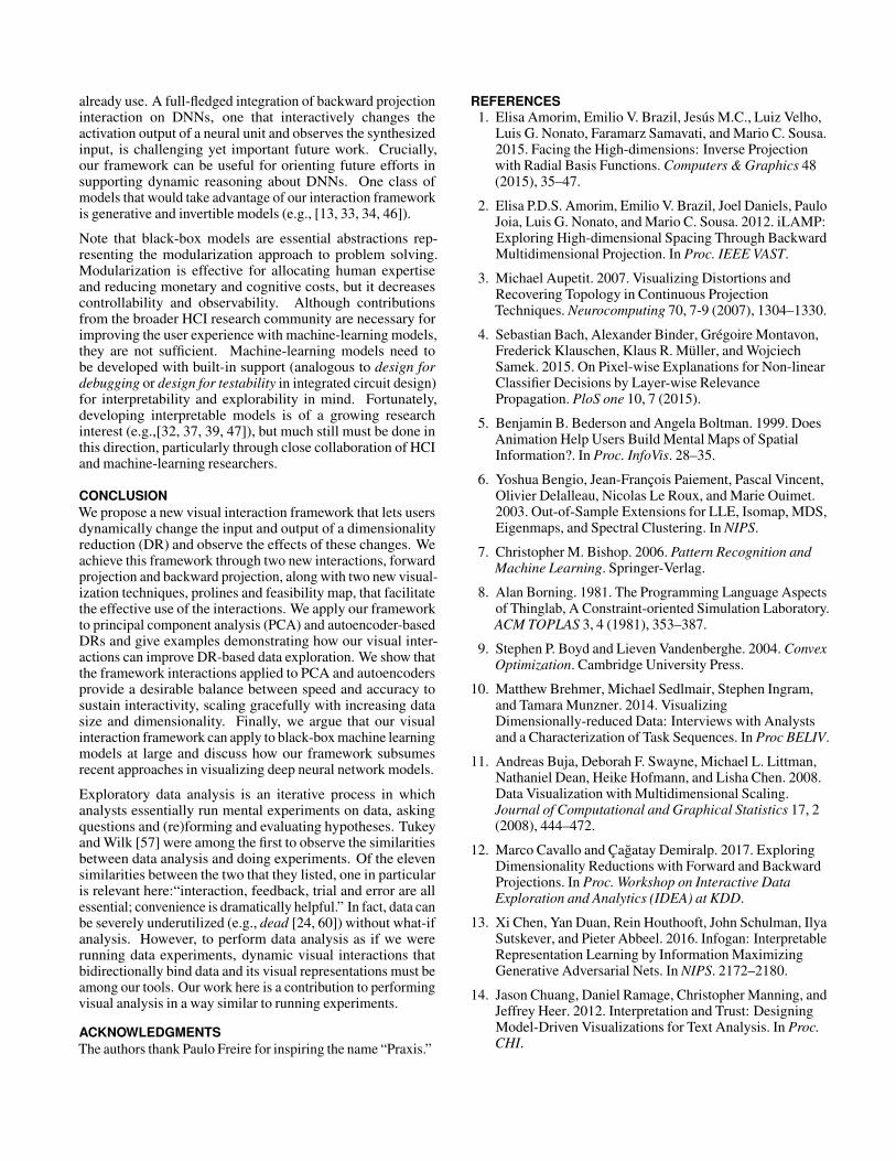
Example: MNISTUmberto, a data-science student, wants to better understandan autoencoder-based DR of the well-known MNIST dataset.From Praxis, he observes the scatter plot of dimensionally re-duced data and notices that similar digits tend to cluster togetheralong different radial directions. He immediately notices anoutlier (a “2”) within a group of “0”s and wants to understandwhich key features (pixels) are determining its position in theprojection plane (Figure 9a). Hovering on the image with themouse highlights the prolines associated with each pixels. Um-berto observes that lower pixel values at the center of the digitwould move the data point down, to within the “0” cluster; con-versely, increasing pixel values in the bottom-right corner of theimage would move the data point up, towards the other “2”s. Hehypothesizes that putting a tail on the digit would make it lookmore like a “2” and verifies this through forward projection:coloring the appropriate pixels (i.e., increasing their featurevalues) moves the data point away from the cluster of “0”s.

Umberto now observes how certain regions of the plane arequite dense, while other regions contain very few data samples.He selects a data point from the “0” cluster and drags it into anempty region at the border of the projection plane (Figure 9b).While dragging the point, he observes how the pixel valuesupdate, showing alternately features of a “0” and of a “7”, thetwo digits whose clusters are closest to this region of the plane.

Input image(28x28 pixels)

Input Layer784 nodes

… …Reconstructed image

(28x28 pixels)

… …

Layer #1128 nodes

Layer #5128 nodes

Output Layer784 nodes

Layer #32 nodes

Layer #232 nodes

Layer #432 nodes

CompressedFeatures

. . . . . . .

. . . . .

. . . . .

. . . . . . .

. .

. .

Encoding Layers Decoding Layers

All layers are fully connected

Figure 8: Architecture of the autoencoder trained on theexample datasets. The first three hidden layers of the networkrepresent the encoding function, which generates a compressedversion of the input image. The last two hidden layers andthe output layer represent the decoding function, which aimsat reconstructing the original image from its compressedrepresentation.

Example: QuickDrawAlice, a data scientist, is excited about the recent release ofGoogle Quick Draw dataset and would like to apply DR toa subset (10) of the image categories in the dataset. Whileperforming her analysis with Praxis, she decides to focus on anisolated data point corresponding to the image of an airplane.By filtering its prolines in order to show only the 100 longestones, Alice can observe which features (pixels) are most influ-ential in determining the position of the image in the projectionplane (Figure 9c). In particular, she notices a smaller set ofprolines associated to two vertical strips of pixels, suggestingthat an increase in their values would move the airplane towardsthe cluster of beds. Alice decides to perform forward projectionand draws two “legs” at the extremes of the airplane: sheverifies that the data point has now moved in the “bed” cluster.

Continuing her search for outliers, Alice notices a bed thatis apart from the others, probably because it was drawn withonly one leg. She wants to see which other images in thedataset may contain a similar shape and uses the brush todefine inequality constraints on a set of pixels (Figure 9d):all solutions with pixel values of interest below a specificthreshold are not considered acceptable.This way, Alice candirectly observe from the admissible region of feasibility mapthat this particular shape can be found only among bed images.

Example: Fashion MNISTMark, an analyst working for a growing apparel company,wants to understand how fashion articles can be better cate-gorized on the company’s website on the basis of their image.He uses Praxis to apply autoencoder-based dimensionalityreduction on the dataset and notices that the projection planeshows a clear separation of footwear data samples from clothes.The two clusters are set apart by a diagonal group of bagswhose images have a distinctive rectangular shape.

Mark wants to explore first the region of the plane containingshoes. He selects a boot data sample that appears as an outlierand brings it towards the cluster of points with the same labelthrough backward projection (Figure 9e). Mark notices thatthe neck of the boot becomes shorter, meaning that the boot’soriginal height was above average. He hypothesizes that theheight of a shoe is a critical factor in determining its positionin the projection plane. He then drags the same data pointclose to the cluster of sneakers and watches the pixels of theimage modify so that the boot gets even shorter, validating hishypothesis. Moreover, he notices that the boot has become flat,losing its characteristic heel. Finally, wanting to understandwhat distinguishes sandals from shoes and boots, he continuesdragging the data point through backward projection. As hedoes so, he notices that the pixel density of the image decreasessignificantly while moving along the main diagonal of theprojection plane. Indeed, sandals prove to be the class ofimages with the fewest colored pixels, because they are openshoes and require less material for construction.

By observing the projection plane, Mark notes that dressesinterestingly fall in a region very close to the cluster of trousers.He then selects a dress and observes that many of its (red)prolines are directed towards that cluster, indicating a decreasein pixel values. By hovering these prolines, Mark observes

MNIST QuickDraw Fashion MNIST

Figure 9: Application of our framework to autoencoder-based data exploration. MNIST: identification of relevant features foran unclear digit through prolines and forward projection (a); exploration of latent space at the borders of the projection plane (b).QuickDraw: prolines show that adding legs to an airplane would make it look more like a bed (c); by setting minimum constraintson the values of a set of pixels (colored in red), the feasibility map shows images similar to the current one (d). Fashion MNIST:the difference between dresses and trousers is explored through forward projection (e); key features differentiating various typesof footwear are explored through backward projection (f).

that they correspond to the central region of the dress image.Through forward projection, he erases those pixels (i.e., setstheir feature value to zero), making the dress image looklike a pair of trousers (Figure 9e). He then observes how thedata point quickly moved into the cluster of trousers. Finally,Mark asks himself where a skirt would be positioned in theprojection plane if the dataset contained one. So he selectsanother dress data sample and erases the upper part of its image,shaping a skirt. Noticing how little the data point has moved,he hypothesizes that skirts would cluster with dresses.

DISCUSSION

Scalability and AccuracyScalability is a fundamental aspect of any visual interactiontechnique that can handle large datasets. We design the visualinteractions supporting our framework with scalability in mind.Our analysis indicates (Figure 10) that our forward and back-ward projection implementations for PCA and autoencoderprovide a desirable tradeoff between accuracy and speed.

To assess the performance of the framework interactionsapplied to PCA and autoencoder dimensionality reductions(DRs), we measure the speed and accuracy of forward andbackward projections on varying number of data samplesand dimensions (see Supplementary Material for details andadditional results). For this, we first generate a syntheticdataset by sampling from a multivariate Gaussian distributionwith sufficiently large dimensions. We then programmaticallyinduce a change of σi/8 for forward projections and m/80 forbackward projections, where σi is the standard deviation of theith dimension in the dataset and m is the width of the projection

plane. When varying the number of samples, we keep the num-ber of dimensions constant at 10. Conversely, when varying thenumber of dimensions, we set the number of samples to 100.

Figure 10 (left) suggests that the time required to computeforward and backward projections for interactive applications(~20 microseconds) is not significantly affected by inputsize. We note that recomputing the DR without out-of-sampleextension is several orders of magnitude slower, especially inthe case of autoencoder networks.

To measure accuracy, we compute two sets of neighbors ona data point for each performance of our interactions: 1) thek-nearest neighbors in the projection plane after performing aforward or a backward projection and 2) the k-nearest neighborsin the projection plane after recomputing dimensionalityreduction on the multidimensional data. We set k=10 for theresults shown in Figure 10. Ideally, these two neighborhoodsshould contain the same elements and the elements should havethe same relative distance from the data point on which theinteraction is performed. We use a correlation index to quantifythe similarity of these two neighborhoods, considering boththe number of overlapping elements and the rank order oftheir distances from the point. Figure 10 (right) shows that theaccuracy decreases sublinearly with the input size. On the otherhand, the accuracy as measured by our correlation index iseither unaffected or slightly improved by the increasing numberof dimensions, since the probability of a single attribute changeaffecting the neighborhood formation and ranking decreaseswith the increasing number of dimensions.

What about visual scalability? Rendering large numberof prolines for high-dimensional datasets can be slow andcan clutter the projection view. Sampling and bundling

PCA

Aut

oenc

oder

~20µs ~20µs

~20µs ~20µs

~2s ~2s

Time required by recomputing

Time required by FP/BP

Retraining the autoencoder is expensive

High accuracy means FP and BP preserve the neighborhood of the data point they are applied to

Recomputation

Backward Projection (BP)

Forward Projection (FP)Forward Projection (FP)

Backward Projection (BP)

Number of dimensionsNumber of samples

Number of dimensionsNumber of samples

Number of dimensionsNumber of samples

Number of dimensionsNumber of samples

Ave

rage

tim

e (µ

s)

Ave

rage

tim

e (µ

s)A

vera

ge ti

me

(ms)

Ave

rage

tim

e (m

s)

Ave

rage

cor

rela

tion

Ave

rage

cor

rela

tion

Ave

rage

cor

rela

tion

Ave

rage

cor

rela

tion

Time Accuracy

Figure 10: Time and accuracy performance of forward and backward projections for PCA and autoencoder-based dimensionalityreductions. Time performance results (left) show how out-of-sample extension outperforms recomputation, guaranteeing lowlatency even with increasing input size. Accuracy performance results (right) demonstrate how forward and backward projectionprovide a desirable tradeoff of accuracy and speed.

(aggregation) [17] can help address this problem. Taking asampling approach, Praxis shows the top-k most “important”prolines when there are too many to draw (Figure 9c).

An important consideration related to accuracy is trust. Whilewe focus here on interpretability through dynamic reasoningand experimentation, trust is also an important design criterionfor model-based visual analysis [14]. How best to conveythe approximation accuracy of our visual interactions to userwithout degrading computational and visual scalability orinserting additional layer of complexity is an important avenueof future research.

Extending the FrameworkAlthough we focus on DR here, our framework can apply toblack-box models in general. Neural network models withmultiple hidden layers (or deep neural networks, DNNs) area particularly popular class of black-box machine learningmodels, and they have recently achieved dramatic successes.However, formal understanding of these models is limited,and the fact that they can easily have millions of parameterswith increasingly intricate architectures only exacerbates theproblem. Researchers have recently turned to visualization togain insights into deep learning models. Prior work applyingvisualization to improve the understanding and interpretabilityof deep neural networks shows patterns that fit well in ourframework, attesting to its ecological validity and extensibility.

We can group DNN visualization approaches into two broadclasses [65]: The first approach is to visualize how the networkresponds to a specific input in order to explain a particular

prediction by the network (e.g.,[4, 40, 42, 53, 54, 62, 63, 64,65]). A common technique used for convolutional neuralnetworks for computer vision applications is to occlude parts ofinput images and observe how the output activation results (e.g.,classification) change [62, 63]. This is an instance of a forwardprojection, changing the input and observing the output change,albeit performed non-interactively in general, with one notableexception [62]. Another common visualization in this approachis saliency maps. Motivated similarly to prolines, saliencymaps visualize which features (e.g., pixels) contribute to theoutput or any other neural unit activation [54, 64, 65].

The second approach is to generate an input that maximallyactivates a given unit or, say, class score to visualize what thenetwork is looking for in making predictions (e.g.,[21, 35, 36,45, 54, 62]). Techniques within this approach aim to synthesizeinput based on a maximization constraint and can be consideredan instance of backward projection. DNN researchers alsorecognize the importance of semantic constraints (e.g., naturalimage priors) in computing backward projections.

Visualization techniques within the two approaches abovehave been developed primarily by machine-learning andcomputer-vision researchers to address their research questionsand to understand and communicate the behavior of theirmodels. These techniques are typically computed throughcommand- line interaction and viewed as static images, withlimited or no interactivity. Applying dynamic interactionsof our framework to DNNs can significantly improve theeffectiveness of the visualization techniques DNN researchers

already use. A full-fledged integration of backward projectioninteraction on DNNs, one that interactively changes theactivation output of a neural unit and observes the synthesizedinput, is challenging yet important future work. Crucially,our framework can be useful for orienting future efforts insupporting dynamic reasoning about DNNs. One class ofmodels that would take advantage of our interaction frameworkis generative and invertible models (e.g., [13, 33, 34, 46]).

Note that black-box models are essential abstractions rep-resenting the modularization approach to problem solving.Modularization is effective for allocating human expertiseand reducing monetary and cognitive costs, but it decreasescontrollability and observability. Although contributionsfrom the broader HCI research community are necessary forimproving the user experience with machine-learning models,they are not sufficient. Machine-learning models need tobe developed with built-in support (analogous to design fordebugging or design for testability in integrated circuit design)for interpretability and explorability in mind. Fortunately,developing interpretable models is of a growing researchinterest (e.g.,[32, 37, 39, 47]), but much still must be done inthis direction, particularly through close collaboration of HCIand machine-learning researchers.

CONCLUSIONWe propose a new visual interaction framework that lets usersdynamically change the input and output of a dimensionalityreduction (DR) and observe the effects of these changes. Weachieve this framework through two new interactions, forwardprojection and backward projection, along with two new visual-ization techniques, prolines and feasibility map, that facilitatethe effective use of the interactions. We apply our frameworkto principal component analysis (PCA) and autoencoder-basedDRs and give examples demonstrating how our visual inter-actions can improve DR-based data exploration. We show thatthe framework interactions applied to PCA and autoencodersprovide a desirable balance between speed and accuracy tosustain interactivity, scaling gracefully with increasing datasize and dimensionality. Finally, we argue that our visualinteraction framework can apply to black-box machine learningmodels at large and discuss how our framework subsumesrecent approaches in visualizing deep neural network models.

Exploratory data analysis is an iterative process in whichanalysts essentially run mental experiments on data, askingquestions and (re)forming and evaluating hypotheses. Tukeyand Wilk [57] were among the first to observe the similaritiesbetween data analysis and doing experiments. Of the elevensimilarities between the two that they listed, one in particularis relevant here:“interaction, feedback, trial and error are allessential; convenience is dramatically helpful.” In fact, data canbe severely underutilized (e.g., dead [24, 60]) without what-ifanalysis. However, to perform data analysis as if we wererunning data experiments, dynamic visual interactions thatbidirectionally bind data and its visual representations must beamong our tools. Our work here is a contribution to performingvisual analysis in a way similar to running experiments.

ACKNOWLEDGMENTSThe authors thank Paulo Freire for inspiring the name “Praxis.”

REFERENCES1. Elisa Amorim, Emilio V. Brazil, Jesús M.C., Luiz Velho,

Luis G. Nonato, Faramarz Samavati, and Mario C. Sousa.2015. Facing the High-dimensions: Inverse Projectionwith Radial Basis Functions. Computers & Graphics 48(2015), 35–47.

2. Elisa P.D.S. Amorim, Emilio V. Brazil, Joel Daniels, PauloJoia, Luis G. Nonato, and Mario C. Sousa. 2012. iLAMP:Exploring High-dimensional Spacing Through BackwardMultidimensional Projection. In Proc. IEEE VAST.

3. Michael Aupetit. 2007. Visualizing Distortions andRecovering Topology in Continuous ProjectionTechniques. Neurocomputing 70, 7-9 (2007), 1304–1330.

4. Sebastian Bach, Alexander Binder, Grégoire Montavon,Frederick Klauschen, Klaus R. Müller, and WojciechSamek. 2015. On Pixel-wise Explanations for Non-linearClassifier Decisions by Layer-wise RelevancePropagation. PloS one 10, 7 (2015).

5. Benjamin B. Bederson and Angela Boltman. 1999. DoesAnimation Help Users Build Mental Maps of SpatialInformation?. In Proc. InfoVis. 28–35.

6. Yoshua Bengio, Jean-François Paiement, Pascal Vincent,Olivier Delalleau, Nicolas Le Roux, and Marie Ouimet.2003. Out-of-Sample Extensions for LLE, Isomap, MDS,Eigenmaps, and Spectral Clustering. In NIPS.

7. Christopher M. Bishop. 2006. Pattern Recognition andMachine Learning. Springer-Verlag.

8. Alan Borning. 1981. The Programming Language Aspectsof Thinglab, A Constraint-oriented Simulation Laboratory.ACM TOPLAS 3, 4 (1981), 353–387.

9. Stephen P. Boyd and Lieven Vandenberghe. 2004. ConvexOptimization. Cambridge University Press.

10. Matthew Brehmer, Michael Sedlmair, Stephen Ingram,and Tamara Munzner. 2014. VisualizingDimensionally-reduced Data: Interviews with Analystsand a Characterization of Task Sequences. In Proc BELIV.

11. Andreas Buja, Deborah F. Swayne, Michael L. Littman,Nathaniel Dean, Heike Hofmann, and Lisha Chen. 2008.Data Visualization with Multidimensional Scaling.Journal of Computational and Graphical Statistics 17, 2(2008), 444–472.

12. Marco Cavallo and Çagatay Demiralp. 2017. ExploringDimensionality Reductions with Forward and BackwardProjections. In Proc. Workshop on Interactive DataExploration and Analytics (IDEA) at KDD.

13. Xi Chen, Yan Duan, Rein Houthooft, John Schulman, IlyaSutskever, and Pieter Abbeel. 2016. Infogan: InterpretableRepresentation Learning by Information MaximizingGenerative Adversarial Nets. In NIPS. 2172–2180.

14. Jason Chuang, Daniel Ramage, Christopher Manning, andJeffrey Heer. 2012. Interpretation and Trust: DesigningModel-Driven Visualizations for Text Analysis. In Proc.CHI.

15. Danilo B. Coimbra, Rafael M. Martins, Tácito T.A.T.Neves, Alexandru C. Telea, and Fernando V. Paulovich.2016. Explaining Three-dimensional DimensionalityReduction Plots. Information Visualization 15, 2 (2016),154–172.

16. Tarik Crnovrsanin, Chris Muelder, Carlos Correa, andKwan-Liu Ma. 2009. Proximity-based Visualization ofMovement Trace Data. In Proc. IEEE VAST.

17. Renato R.O. da Silva, Paulo E. Rauber, and Alexandru C.Telea. 2016. Beyond the Third Dimension: VisualizingHigh-dimensional Data with Projections. Computing inScience & Engineering 18, 5 (2016), 98–107.

18. Çagatay Demiralp. 2016. Clustrophile: A Tool for VisualClustering Analysis. In KDD IDEA.

19. Alex Endert, Patrick Fiaux, and Chris North. 2012.Semantic Interaction for Visual Text Analytics. In Proc.CHI.

20. Alex Endert, Chao Han, Dipayan Maiti, Leanna House,and Chris North. 2011. Observation-level Interaction WithStatistical Models for Visual Analytics. In Proc. IEEEVAST.

21. Dumitru Erhan, Yoshua Bengio, Aaron Courville, andPascal Vincent. 2009. Visualizing Higher-Layer Featuresof a Deep Network. Technical Report 1341. University ofMontreal.

22. Karl Ruben Gabriel. 1971. The Biplot Graphic Display ofMatrices with Application to Principal ComponentAnalysis. Biometrika (1971), 453–467.

23. Michael Gleicher. 2013. Explainers: Expert Explorationswith Crafted Projections. IEEE TVCG 19, 12 (2013),2042–2051.

24. Peter J. Haas, Paul P. Maglio, Patricia G. Selinger, andWang C. Tan. 2011. Data is Dead. . . Without What-ifModels. PVLDB 4, 12 (2011), 1486–1489.

25. Trevor Hastie, Robert Tibshirani, Jerome Friedman, andJames Franklin. 2005. The Elements of StatisticalLearning: Data Mining, Inference and Prediction. TheMathematical Intelligencer 27, 2 (2005), 83–85.

26. Geoffrey E. Hinton and Ruslan R. Salakhutdinov. 2006.Reducing the Dimensionality of Data with NeuralNetworks. Science 313, 5786 (2006), 504–507.

27. Edwin L. Hutchins, James D. Hollan, and Donald A.Norman. 1985. Direct Manipulation Interfaces.Human–Computer Interaction 1, 4 (1985), 311–338.

28. Dong H. Jeong, Caroline Ziemkiewicz, Brian Fisher,William Ribarsky, and Remco Chang. 2009. iPCA: AnInteractive System for PCA-based Visual Analytics.Computer Graphics Forum 28, 3 (2009), 767–774.

29. Sara Johansson and Jimmy Johansson. 2009. InteractiveDimensionality Reduction Through User-definedCombinations of Quality Metrics. IEEE TVCG 15, 6(2009), 993–1000.

30. Paulo Joia, Danilo Coimbra, Jose A. Cuminato,Fernando V. Paulovich, and Luis G. Nonato. 2011. LocalAffine Multidimensional Projection. IEEE TVCG 17, 12(2011), 2563–2571.

31. Alan Kay and Adele Goldberg. 1977. Personal DynamicMedia. Computer 10, 3 (1977), 31–41.

32. Been Kim, Julie A. Shah, and Finale Doshi-Velez. 2015.Mind the Gap: A Generative Approach to InterpretableFeature Selection and Extraction. In NIPS. 2260–2268.

33. Diederik P. Kingma and Max Welling. 2013.Auto-encoding Variational Bayes. arXiv preprintarXiv:1312.6114 (2013).

34. Guillaume Lample, Neil Zeghidour, Nicolas Usunier,Antoine Bordes, Ludovic Denoyer, and Marc’AurelioRanzato. 2017. Fader Networks: Manipulating Images bySliding Attributes. arXiv preprint arXiv:1706.00409(2017).

35. Quoc V. Le, Marc’Aurelio Ranzato, Rajat Monga,Matthieu Devin, Kai Chen, Greg S. Corrado, Jeff Dean,and Andrew Y. Ng. 2012. Building High-level FeaturesUsing Large Scale Unsupervised Learning. In Proc. ICML.

36. Honglak Lee, Chaitanya Ekanadham, and Andrew Y. Ng.2007. Sparse Deep Belief Net Model for Visual Area V2.In NIPS.

37. Tao Lei, Regina Barzilay, and Tommi Jaakkola. 2016.Rationalizing Neural Predictions. Proc. EMNLP (2016).

38. Sylvain Lespinats and Michael Aupetit. 2010. CheckViz:Sanity Check and Topological Clues for Linear andNon-Linear Mappings. Computer Graphics Forum 30, 1(2010), 113–125.

39. Benjamin Letham, Cynthia Rudin, Tyler H. McCormick,David Madigan, and others. 2015. Interpretable ClassifiersUsing Rules and Bayesian Analysis: Building a BetterStroke Prediction Model. The Annals of Applied Statistics9, 3 (2015), 1350–1371.

40. Jiwei Li, Xinlei Chen, Eduard Hovy, and Dan Jurafsky.2015. Visualizing and Understanding Neural Models inNLP. arXiv preprint arXiv:1506.01066 (2015).

41. Laurens van der Maaten and Geoffrey Hinton. 2008.Visualizing Data Using t-SNE. Journal of MachineLearning Research 9 (2008), 2579–2605.

42. Aravindh Mahendran and Andrea Vedaldi. 2015.Understanding Deep Image Representations by InvertingThem. In CVPR.

43. Gladys M.H. Mamani, Francisco M. Fatore, Luis G.Nonato, and Fernando V. Paulovich. 2013. User-drivenFeature Space Transformation. Computer Graphics Forum32 (2013), 291–299.

44. Nathan D. Monnig, Bengt Fornberg, and Francois G.Meyer. 2014. Inverting Nonlinear DimensionalityReduction with Scale-free Radial Basis FunctionInterpolation. Applied and Computational HarmonicAnalysis 37, 1 (2014), 162–170.

45. Anh Nguyen, Jason Yosinski, and Jeff Clune. 2016.Multifaceted Feature Visualization: Uncovering theDifferent Types of Features Learned by Each Neuron inDeep Neural Networks. (2016).

46. Guim Perarnau, Joost van de Weijer, Bogdan Raducanu,and Jose M. Álvarez. 2016. Invertible Conditional GANsfor Image Editing. arXiv preprint arXiv:1611.06355(2016).

47. Marco T. Ribeiro, Sameer Singh, and Carlos Guestrin.2016. Why Should I Trust you?: Explaining thePredictions of Any Classifier. In Proc. KDD. ACM,1135–1144.

48. David E. Rumelhart, Geoffrey. E. Hinton, and Ronald. J.Williams. 1986. In Parallel Distributed Processing:Explorations in the Microstructure of Cognition, Vol. 1,David E. Rumelhart and James L. McClelland (Eds.).Chapter Learning Internal Representations by ErrorPropagation, 318–362.

49. Dominik Sacha, Leishi Zhang, Michael Sedlmair, John A.Lee, Jaakko Peltonen, Daniel Weiskopf, Stephen C. North,and Daniel A. Keim. 2017. Visual Interaction withDimensionality Reduction: A Structured LiteratureAnalysis. IEEE TVCG 23, 1 (2017), 241–250.

50. Tobias Schreck, Jurgen Bernard, Tatiana vonLandesberger, and Jorn Kohlhammer. 2009. Visual ClusterAnalysis of Trajectory Data with Interactive KohonenMaps. Information Visualization 8, 1 (2009), 14–29.

51. Michael Sedlmair, Tamara Munzner, and Melanie Tory.2013. Empirical Guidance on Scatterplot and DimensionReduction Technique Choices. IEEE TVCG 19, 12 (2013),2634–2643.

52. Ben Shneiderman. 1983. Direct Manipulation: A StepBeyond Programming Languages. Computer 16, 8 (1983),57–69.

53. Avanti Shrikumar, Peyton Greenside, Anna Shcherbina,and Anshul Kundaje. 2016. Not Just a Black Box:Learning Important Features Through PropagatingActivation Differences. arXiv preprint arXiv:1605.01713(2016).

54. Karen Simonyan, Andrea Vedaldi, and Andrew Zisserman.2013. Deep Inside Convolutional Networks: VisualisingImage Classification Models and Saliency Maps. (2013).

55. Julian Stahnke, Marian Dörk, Boris Müller, and AndreasThom. 2016. Probing Projections: Interaction Techniquesfor Interpreting Arrangements and Errors ofDimensionality Reductions. IEEE TVCG 22, 1 (2016),629–638.

56. Ivan E. Sutherland. 1963. Sketchpad: A Man-machineGraphical Communication System. In Proc. Spring JointComputer Conference.

57. John W. Tukey and Martin B. Wilk. 1966. Data Analysisand Statistics: An Expository Overview. In Proc. FallJoint Computer Conference.

58. Laurens van der Maaten, Eric Postma, and Japp van denHerik. 2009. Dimensionality Reduction: A ComparativeReview. Technical Report. TiCC, Tilburg University.

59. Christophe Viau, Michael J. McGuffin, Yves Chiricota,and Igor Jurisica. 2010. The FlowVizMenu and ParallelScatterplot Matrix: Hybrid MultidimensionalVisualizations for Network Exploration. IEEE TVCG(2010), 1100–1108.

60. Bret Victor. 2013. Media for Thinking the Unthinkable.https://vimeo.com/67076984. (2013). Accessed: Dec24th, 2017.

61. Matt Williams and Tamara Munzner. 2004. Steerable,Progressive Multidimensional Scaling. In Proc. IEEEInfoVis.

62. Jason Yosinski, Jeff Clune, Anh Nguyen, Thomas Fuchs,and Hod Lipson. 2015. Understanding Neural NetworksThrough Deep Visualization. (2015).

63. Matthew D. Zeiler and Rob Fergus. 2014. Visualizing andUnderstanding Convolutional Networks. In Proc. ECCV.

64. Bolei Zhou, Aditya Khosla, Agata Lapedriza, Aude Oliva,and Antonio Torralba. 2016. Learning Deep Features forDiscriminative Localization. In CVPR.

65. Luisa M. Zintgraf, Taco S. Cohen, Tameem Adel, and MaxWelling. 2017. Visualizing Deep Neural NetworkDecisions: Prediction Difference Analysis. In Proc. ICLR.