a web-based system for optimizing post disaster temporary

A Web-based System for Optimizing Post Disaster Temporary Housing Allocation

Lei Chen

A thesis

submitted in partial fulfillment of the

requirements for the degree of

Master of Science in Industrial Engineering

University of Washington

2012

Committee:

Zelda B. Zabinsky

Omar El-Anwar

Joseph A. Heim

Program Authorized to Offer Degree:

Industrial & Systems Engineering

University of Washington

ABSTRACT

Thesis Title: A Web-based System for Optimizing Post Disaster Temporary Housing Allocation

Lei Chen

Chair of the Supervisory Committee:

Zelda B. Zabinsky

Omar El-Anwar

Natural catastrophes can result in large scale displacement of populations, who are in urgent

need of temporary quarters until permanent housing can be provided. During this period, the

temporary housing plays an important role in the families’ physical, psychological, social and

economic recovery. A number of research studies have addressed this specific temporary

housing problem and aimed at identifying the optimal temporary housing arrangements, but few

used quantitative methods to incorporate the displaced families’ specific socioeconomic needs

and housing preferences. From the decision makers’ perspective, current temporary housing

practices often result in high cost, late delivery and frequent family complaints caused by

improper allocation. The scale and complexity of the problem requires strategic planning and a

fast decision support system.

The main objective of this thesis is to present a way of effectively matching available temporary

housing resources to displaced families’ social, economic and psychological needs with the

minimum required public expenditure. A new web-based post disaster temporary housing

management system is developed to accomplish this task. It fully considers individual family’s

specific needs and provides comprehensive decision support.

The web-based system first solicits and stores the data from potential housing providers. It

applies Google Map® in the user interface to facilitate data acquisition. The collected families’

needs and preferences are then translated into a socioeconomic index to evaluate housing

alternatives. In order to maximize overall families’ utility and minimize expenditure, a multi-

objective optimization module is formulated using the classic weighted sum method. A

customized Hungarian Algorithm is developed to solve the optimization problem. In addition,

the system also provides decision support for the total cost and overall socioeconomic benefit

trade off and cost-benefit analysis for various potential housing.

The web-based system can significantly improve the current temporary housing practices. It has

a user friendly interface and allows families to better describe their requirements. With the

customized Hungarian Algorithm the optimization process won’t cause computer out of memory

in the large scale problems and it saves significant running time. The computational speed and

efficiency of the system enables its use in the response phase following a disaster, where it can

offer high quality allocation solutions with low cost.

i

TABLE OF CONTENTS

Page

List of Figures……………………………………………………………………………ii

List of Tables………………………………………………………………………….....iii

Acknowledgements……………………………………………………………………...iv

Chapter I: Introduction……………………………...……………….…………………...1

Overview and Problem Statement………………………………………..1

Literature Review………………………………………………………...1

Research Objectives and Research Methodology...………. ……………..2

Thesis Organization………………………………………………………3

Chapter I: Data Acquisition Module……………………………….…………………….5

Displaced Family Portals………………………………………………....5

Housing Provider Portals…………………………………………………6

Emergency Management Agency Portals………………………………...8

Database…………………………………………………………………..9

Chapter II: Data Analysis Module………………………………………………………10

Displacement Distance Equivalent Index………………………………..11

Housing Characteristics Index…………………………………………...13

Socioeconomics Index…………………………………………………...14

Life time Cost……………………………………………………………15

Chapter III: Multi-Objective Optimization Module……………………………………..16

Optimization Formulation……………………………………………….17

Optimization Algorithm………………………………………………….21

Chapter IV: Decision Support Module…………………………………………………..31

Cost Benefit Analysis…………………………………………………....31

Potential Housing Analysis………………………………………………32

Chapter V: Output Reporting Module…………………………………………………...33

Chapter VI: Conclusion………………………………………………………………….36

Bibliography……………………………………………………………………………..37

Appendix: PHP Code for Customized Hungarian Algorithm…………………………....42

ii

LIST OF FIGURES

Page

1.1. General Structure of the system ……………...……………………………………....3

2.1. Structure of Module 1………………………… ………………………………...…...5

2.2. Input Interface for Housing Providers.…………………………………………….…6

2.3. Information about Housing alternatives………………………………………………7

2.4. Input Interface for Displaced Families.…………………………………………...….8

2.5. Database Structure…………………………………………………………………....9

3.1. Structure of Module 2……………………………………………………………….11

3.2. Utility Functions Used to Compute the Displacement Distance Equivalency Index.12


4.2. Pareto Optimal Solution……………………………………………………………..18

4.3. Algorithm Case Example………………………………………………………...….27

4.4. Solutions for the Case Example…………………………………………………......30


5.2. Cost-Benefit Analysis…………………………………………………………...…..32

5.3. Potential Housing Analysis……………………………………………………...…..33

6.1. Family Output Portal……………………………………………………………...…34

6.2. Family List for a Housing Provider……………………………………………........35

6.3. Output Tables for Emergency Management Agency……………………………......35

iii

LIST OF TABLES

Page

4.1. Weight Table …………………………………………………………………...…...21

4.2. Weight Table for Temporary Housing Problem………….……………………...….22

4.3. Algorithm Performance Comparison……………………………………………......29

4.4. Optimization Results………………………………………………………………...30

iv

ACKNOWLEDGEMENTS

The author wishes to express sincere appreciation to the Department of Industrial & Systems

Engineering for their extended long-term support and especially to Professor Zelda B. Zabinsky

and Professor Omar El-Anwar for their patience and great knowledge. This thesis would never

have been completed without the encouragement of my parents.

1

I. INTRODUCTION

1.1. Overview and Problem Statement

Natural catastrophes can cause large scale displacement of populations, who are in urgent

need for temporary quarters until new permanent housing can be provided or their pre-

disaster housing can be repaired. During this critical period, the temporary housing

location plays a significant role in the displaced family’s psychological, social, and

economic recovery. When selecting the housing location it is essential to meet a number

of needs (which can vary from household to another), such as proximity to jobs, kinship

ties, educational facilities (K-12 and/or higher education), social support networks,

religious groups, healthcare facilities, and public transportation and important services

(Bolin and Bolton 1986; El-Anwar et al. 2008; El-Anwar et al. 2010c; FEMA 2005a;

FEMA 2005b; FEMA 2007; Hidayat and Egbu 2010; Johnson 2002a; Johnson 2002b;

Quercia and Bates 2002; Rakes et al. 2010; Shlay 1995). The poor selection of temporary

housing locations can add to the displaced families’ compound stresses after the disaster

and disrupt their neighborhood patterns, social support networks, and familiar

surroundings (Bolin and Bolton 1986). The inability to meet the families’ needs can

result in a wide range of consequences; starting from families rejecting the offered

temporary housing because of its unreasonable distance from their jobs and ending by

high suicide rates due to loneliness and despair attributed to being cut off from their

communities (Comerio 1998; Johnson 2007; Tomioka 1997).

For decades, post-disaster temporary housing programs have been criticized for their

inability to meet the expectations of displaced populations. This criticism stems from

various reasons, including (1) the temporary housing late delivery (Bolin 1993; Friday

1999; Johnson 2007); (2) inability to fulfill the social, psychological, and economic needs

of displaced families (Bolin 1982; Bolin and Bolton 1986; Comerio 1998; Friday 1999;

Golec 1983; Johnson 2007; Lizarralde and Johnson 2003; Tomioka 1997); and (3) poor

accessibility of temporary housing locations to essential services and public

transportation (Bolin 1993). Despite their poor performance, many temporary housing

programs tend to be expensive, which draws from the limited budgets available for

recovery and reconstruction (Friday 1999; Johnson 2002a).

1.2. Literature Review and Research Gap

A number of research studies have addressed the specific problem of identifying the

optimal configurations of temporary housing arrangements in a timely manner following

disasters. Three representative types of models are explained as follow:

2

Model 1: The first model aims to achieve a specific type of objective, which includes

maximizing temporary housing structural safety (El-Anwar et al 2010a), minimizing the

environmental impacts of constructing and maintaining post-disaster accelerated housing

projects (El-Anwar et al 2010b) and minimizing the distance between the assigned

temporary housing and the preferred location by families (El-Anwar and El-Rayes 2007).

Model 2: The second model was designed to identify the optimal locations and types of

temporary housing in order to achieve various socioeconomic, safety, environmental, and

cost objectives (El-Anwar et al. 2009b; Kandil et al. 2010). Despite the significant

contributions of this formulation to improving temporary housing practices, it did not aim

at capturing the specific needs of each displaced family. In this case, the number of

decision variables was equal to the number of available temporary housing alternatives

( ).

Model 3: The third model maintained the same optimization objectives as Model 2.

However, it categorized the families based on their preferred locations for temporary

housing (e.g., zip codes or census tracts), and the corresponding optimization models

accounted for these preferences when optimizing temporary housing assignments (El-

Anwar et al. 2009a; El-Anwar et al. 2010; McLaren at al. 2009). Accordingly, the

decision variables for this formulation were equal to the number of available temporary

housing alternatives ( ) multiplied by the number of preferred housing locations ( )

resulting in a running time in the order of one hour on consumer-grade computers.

Despite the significant contributions of the aforementioned models in optimizing

temporary housing arrangements, there is a need for an innovative methodology that can

explicitly account for the displacement distance and housing characteristics from various

socioeconomic needs and effectively evaluate housing assignments based on the

individual needs of each family.

Besides, as the complexity of the model increases, the running time also increases

significantly. The new model, as it attempts to capture each family’s specific

socioeconomic needs as well as temporary housing characteristics and optimize housing

decisions accordingly, will have a challenge to keep the running time in the acceptable

range.

1.3. Research Objectives and Research Methodology

The main objective of this thesis is to present a system which can effectively match

available temporary housing alternatives to displaced families’ social, economic and

psychological needs with the minimum required public expenditure. It should incorporate

sufficient strategic planning so as to reduce the response time. And the system must

3

improve on the disadvantage of current temporary housing practice and offer

comprehensive decision support to the emergency management agencies.

The research methodology can be divided into eight major tasks: 1) conduct

comprehensive literature review; 2) build the interface to effectively capture the specific

needs and preferences of each displaced family; 3) appropriately quantify the

performance of candidate temporary housing configurations in fulfilling the families’

specific needs; 4) account for and control temporary housing projects life cycle costs; 5)

develop a multi-objective optimization model to maximize families utility while

minimizing the life cycle cost; 6) minimize the computational requirements or find an

efficient algorithm when solving the associated large-scale optimization problem; 7)

provide adequate decision support tools for decision makers; and 8) report the output to

the families and housing providers once the decision is made. In order to accomplish

these tasks, a new integrated post-disaster temporary housing management system is

needed.

The system will have a big contribution in the disaster management field; it transforms

the one-size-fits-all housing program to a need-tailored approach which considers every

displaced family’s needs. Furthermore, the system can be applied in many other contexts

where the problem aims to match the individual demands to various supplies in different

locations. The algorithm developed for the multi-objective optimization is also of great

value in optimizing similar assignment problems. As a result, the systematic approach

and optimization tool makes this thesis a contribution to Industrial and Systems

Engineering as well.

1.4. Thesis Organization

Figure 1.1 shows the general structure of the system and the interrelation among different

modules. The following chapters will describe each module in detail.

Figure 1.1. General Structure of the System

4

Chapter II - Data Acquisition Module: This chapter introduces web portals for data

acquisition from displaced families, housing providers and Emergency Management

Agency. The Emergency Management Agency is the decision maker in the system. A

brief explanation of the database is also presented in this chapter.

Chapter III - Data Analysis Module: This chapter explains how the system processes the

raw data and uses the socio-economic index to evaluate the performance of candidate

temporary housing in fulfilling families’ needs.

Chapter IV- Multi-Objective Optimization Module: This chapter presents the formulation

of the optimization module, and describes the customized Hungarian algorithm.

Chapter V - Decision Support Module: This chapter explains the Cost-Socioeconomic

tradeoff and Potential Housing Cost Benefit Analysis support functions.

Chapter VI - Output Reporting Result: This chapter briefly shows the way that the system

reports the housing assignment to family and display assignment family list to the

housing providers.

5

II. DATA ACQUISITION MODULE

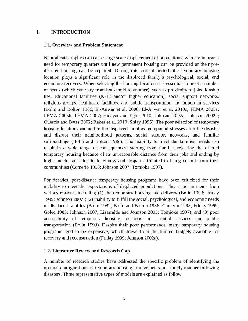
The Data Acquisition Module is the front-end of the web-based system; the objective is

to quickly collect the information necessary to provide families with the housing

solutions that would fulfill their needs. It has three web-portals that serve the Displaced

Families, Housing Providers, and Emergency Management Agencies (as in Figure 2.1).

This section briefly introduces each of the web portals and explains the underlying

database structure. The portals are capable to run in various browsers, and with the fast

development of mobile technology, the module enables the system to quickly identify the

families’ socioeconomic needs and effectively allocate available housing close to the

impacted areas.

Figure 2.1. The Structure of Module 1

2.1.Housing Provider Portal

The Housing Provider Portal is an important component for strategic planning in the

temporary housing management program. It collects all the housing alternative providers’

information prior to disaster occurrence. This housing data allows emergency

management agencies to evaluate the size of the housing market and access a large pool

of housing information immediately after a disaster happens.

The housing alternative providers include hotels, motels, housing rental businesses, etc.

Before any disaster occurs, the data housing providers are invited to input includes: (1)

housing type and address; and (2) housing characteristics such as housing quality using a

pre-defined rating system, level of access to public transportation and other essential

services, neighborhood safety, etc. When a disaster occurs, the emergency management

agencies need to first re-examine the housings, make sure the housing is in good

condition for displaced families. The qualified housing providers are requested to provide

the number of available housing units, their prices and sizes, and availability dates.

6

Figure 2.2. Input Interface for Housing Provider

2.2. Displaced Families Portal

The Displaced Families Portal is the web page for collecting displaced families’ needs

and preference about temporary housing. After disasters happen, the emergency

management agency can provide the URL of the portal to the families. They will be able

to view the housing alternative information, create their account and enter needs and

preference into the system.

Before entering their needs and preference, displaced families can first view the housing

information that the emergency management agency selected. A study suggested that

comprehensive information can significantly reduce human judgment error, which in our

case suggests that the information can guide families to input what truly reflects their

needs and preference (Kruglanski and Icek 1983). The system is able to display location,

quality, neighborhood safety, unemployment rate and key service levels of each housing

(Figure 2.3). Each marker represents a housing alternative, the stars on the marker

indicate the quality level of the housing, and the detail information window pumps up

when the families click one of the markers.

7

Figure 2.3. The Information about Housing Alternatives

The system allows families to create an account. This will expedite the process to collect

information of displaced families, especially in disasters where the number of families

are increasing over time. However, not all of the accounts are necessarily processed, the

emergency management agency needs to verify and organize all the accounts. Only the

selected or filtered accounts will be finally assigned with temporary housing.

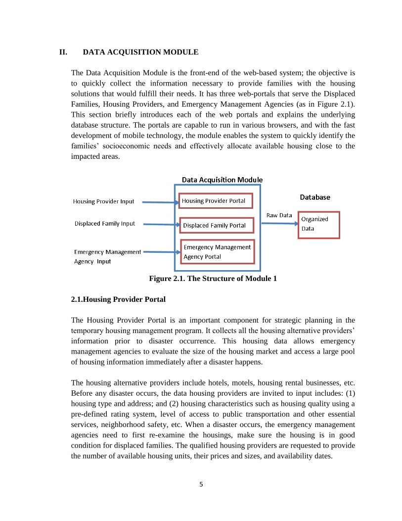
When displaced families apply for temporary housing, they use the portal to provide 3

categories of information. The first category is the location needs, it includes (1) original

family location; (2) preferred location for temporary housing; (3) locations they need to

be close to (e.g., jobs, kinship ties, pre-disaster location, college, etc.); and (4) services

they need to be close to (e.g., K-12 public schools, healthcare and eldercare facilities,

etc.). The second category is the housing characteristics (e.g., safety, housing quality,

access to public services, access to public transportation, etc.). This system requires

families to identify their preferences among their location needs as well as the importance

of the various housing characteristics to them. The system uses the absolute scale (0-

100%) and computes the importance weight for each of the family’s location needs and

housing characteristics. The third category is the overall preference between the location

needs and housing characteristics needs. It also uses the absolute scale (0-100%). Figure

2.4 shows the system screenshot for entering each of the categories of information.

8

Figure 2.4. The Input Interface for Displaced Families

The input window for families is designed as a registration form. The location

identification functions use Google Maps, where families can search the locations with

partial address information (e.g., zip code) or using a drag-and-drop marker. The Google

Map services are fast, simple, and very familiar to most of the families. It has the

advantage of integrated satellite maps, the built in geocoding service provides excellent

accuracy which is very important for the data analysis module.

2.3. Emergency Management Agency Portal

This portal allows emergency management agency planners to retrieve, edit families’ and

housing providers’ data and define decision making parameters. As the administrator of

the system, the planners have the authority to add and delete families and housing

providers’ record. By examining the situation, they can determine the priority of families

and condition of housing alternatives. They also decide which housing information is to

be viewed by the families and the specific types of needs can be selected in the Displaced

Families Portal. The decision making parameters will be discussed more in the Data

Analysis Module, changing those parameters will affect the assignments results.

9

2.4. Database

The database stores the data collected from three web portals as well as the assignment

results when the final decisions are made. The database manages the data in a very

efficient manner, which supports the data analysis module and multi-objective

optimization module to retrieve data.

Figure 2.5 illustrates the overall relational database structure of the system. The

“displaced_family” table contains the basic information of families. The location and

housing characteristics needs of the families are stored in the “need_input” and

“char_need_input” tables, respectively. The “housing” table contains the basic

information of the housing alternatives, where the types of the housing characteristics are

stored in the “housing_char” table. The final assignment table stores the optimization

results, where each family will be assigned one housing unit.

Figure 2.5. Database Structure

10

III. DATA ANALYSIS MODULE

The Data Analysis Module enables the system to use the collected families’ needs to

evaluate all housing alternatives where it calculates a socioeconomic index to represent

the level to which each housing alternative satisfies a family’s socioeconomic needs. The

socioeconomic index will be used later as one of the objective function coefficients in the

multi-objective optimization module.

Before the socioeconomic index can be calculated, it is worthwhile to study some key

factors about temporary housing that can significantly affect the displaced families’

socioeconomic recovery. Previous research suggested that the significant factors include

housing quality, housing delivery time, access to public transportation and other essential

utilities and services, neighborhood safety, proximity to jobs and schools, distance from

pre-disaster location and social support networks, and proximity to healthcare and

eldercare facilities (Bolin and Bolton 1986; Comerio 1997; El-Anwar et al. 2008; El-

Anwar et al. 2010c; FEMA 2005a; FEMA 2005b; FEMA 2007; Friday 1999; Hidayat and

Egbu 2010; Johnson 2002a; Johnson 2002b; Quercia and Bates 2002; Rakes et al. 2010;

Shlay 1995). The Data Analysis Module classifies these socioeconomic factors under two

main categories: (1) displacement distance category, which includes factors that are of

specific interest to some families and are functions in the distance between the proposed

housing and some locations, such as proximity to jobs and schools, distance from pre-

disaster location and social support networks, and proximity to healthcare and eldercare

facilities; and (2) housing characteristics category, which includes the general factors that

are expected to be of interest to all displaced families, such as housing quality, housing

delivery time, access to public transportation and other essential utilities and services, and

neighborhood safety. The families’ location needs collected in the Data Acquisition

Module will be processed to evaluate housing under the displacement distance category,

while the housing characteristics needs are used under the housing characteristics

category.

There are three main phases to calculate the socioeconomic index: (1) identifying the

location needs of displaced families using a displacement distance equivalent index; (2)

computing a housing characteristics index to account for the families’ preferences in

housing characteristics as well as its location attributes; and (3) combining the two

indices to evaluate the overall impact of the each available housing alternative on the

family’s social and economic recovery using a socioeconomic index. In addition to

maximizing socioeconomic benefit, reducing cost is also a key objective of system.

Hence, this module also accounts for the life cycle costs associated with developing each

temporary housing project or procuring housing service. The general structure of this

module is shown in the Figure 3.1.

11

Figure 3.1. The Structure of Module 2

3.1. Displacement Distance Equivalent Index

Housing proximity to families’ needs can significantly impact their socioeconomic

recovery. The displacement distance category is designed to capture these proximity

needs for each family, and it accounts for proximity to (1) location-specific needs, which

are located at specific addresses such as jobs, colleges, kinship ties and other social

support groups, religious facilities, and pre-disaster location; and (2) service-specific

needs, which are offered at multiple facilities at different locations such as K-12

education facilities, hospitals, eldercare facilities, and clinics. This section briefly

describes how the module computes a displacement distance equivalency index to

evaluate the performance of housing alternatives in fulfilling the proximity needs of each

family. There are three steps as discussed below:

First, the module computes the distances between each housing alternative and location-

specific needs entered by each family (e.g., distance to job). Moreover, the module

computes the distances between the housing alternatives and closest service-specific

needs (e.g., closest elementary school). The module currently uses the Haversine Formula

to calculate the shortest distance between each two locations (Sinnott 1984). However,

future developments will include calculating travel distances for more accurate

evaluations.

Second, the module retrieves the family specified preferred location for temporary

housing (e.g., a zip code). If a housing alternative falls within that location, then it will

fulfill a number of the pre-defined proximity needs. Accordingly, in this case the

displacement distance equivalent will be calculated only for needs that do not fall within

the preferred location. However, if a housing alternative is outside the preferred location

area, then the module computes the displacement distance equivalent using all proximity

needs. The module computes the displacement distance equivalent ( ) by

12

aggregating the weighted distances between housing alternative and the needs of family

.

In the third step, the module computes the displacement distance equivalency index

( ) for family and housing alternative thus enabling emergency management

agencies to build a utility function that can be applied to all temporary housing

applications. As shown in Figure 3.2, the utility function is a function in the minimum

displacement , maximum displacement , and a magnifying factor . If

, then we set . Similarly, if , then set

Accordingly, ranges between 0 (lowest performance with

maximum displacement) to 1 (highest performance with minimal or no displacement) and

can be computed using Equation (3.1) below,

Figure 3.2. Utility Functions Used to Compute the Displacement Distance

Equivalency Index for Three Different Magnifying Factors

{

[

]

(3.1)

where,

= displacement distance equivalency index for family residing in housing

alternative ;

= displacement distance equivalent for family residing in housing alternative ;

13

= maximum displacement defined by decision maker to represent the lowest

performance for the location of a temporary housing with respect to fulfilling the

proximity needs of displaced families;

= minimum displacement defined by decision maker to represent the highest

performance for the location of a temporary housing with respect to fulfilling the

proximity needs of displaced families; and

= magnifying factor to represent how the increase in displacement distance impacts the

families socioeconomic welfare.

3.2. Housing Characteristics Index

This subsection briefly describes how the module computes a housing characteristics

index to evaluate the performance of each housing alternative in fulfilling the

socioeconomic needs represented by the factors in the housing characteristics category.

To this end, the module performs three main steps, as follows.

Assessing housing characteristics

The module evaluates the performance of each housing alternative in five main

socioeconomic factors that fall under the housing characteristics category, including (1)

housing quality, which can be rated on a scale from 1 to 5 similar to the hotel rating

system; (2) housing delivery time, which represents how long the displaced families will

stay in mass-care shelters before they can move to temporary housing because of time

needed for construction/installation activities (e.g., for pre-fabricated homes projects) or

room availability (e.g., for motels); (3) level of access of housing location to public

transportation, where decision makers can define five levels of accessibility starting from

“no accessibility” to “highly accessible”; (4) access to other essential utilities and

services, which can follow a similar rating system as access to public transportation and

include access to public services, supermarkets, retail stores, entertainment and

recreational activities; and (5) neighborhood safety, which can be evaluated using

reported crime rates at the temporary housing location. The module normalizes these

ratings using a scale from 0 (lowest performance) to 1 (highest performance) based on a

pre-defined range of values input by the decision making authority for each factor.

Weighting socioeconomic factors

One of the unique features of the proposed module is its ability to capture the specific

preferences of each displaced family among their socioeconomic needs. To this end, the

module asks the families to assign the absolute weight (0-1) to each needs and normalize

it for the five socioeconomic factors.

14

The module computes a housing characteristics index ( ) that represents the

performance of housing alternative in fulfilling the housing characteristics needs of

displaced family . This index is computed by aggregating the weighted performance of

the housing alternative in the five socioeconomic factors, as shown in Equation 3.2 below,

∑

(3.2)

where,

= housing characteristics index representing the evaluated performance of housing

alternative in fulfilling the housing characteristics needs of displaced family , and it

can range from 0% (lowest performance) to 100% (highest performance);

= relative weight of socioeconomic factor computed based on the pair-wise

comparisons performed by family , where there are five factors under the housing

characteristics category; and

= performance of housing alternative in fulfilling socioeconomic need .

3.3. Calculate Socioeconomic Index

The objective of this section is to evaluate the overall socioeconomic performance of

candidate configuration of temporary housing assignments. To this end, the module first

calculates a socioeconomic index ( ) to evaluate the combined social and economic

impacts for each family if they reside in any of the available housing alternatives. The

module computes as the aggregate weighted performance of the temporary housing

alternative in each of and , as shown in Equation (3.3),

(3.3)

where,

= socioeconomic index of family residing in temporary housing alternative ;

= relative weight of housing characteristics for family ; and

= relative weight of displacement distance for family .

Second, in order to evaluate the configuration of all temporary housing assignments, the

module computes an overall socioeconomic index ( ) by averaging the computed

socioeconomic indexes for all the displaced families, as shown in Equation (3.4),

15

∑ ∑

(3.4)

where,

= overall socioeconomic index for a candidate configuration of temporary housing

assignments;

= number of displaced families applying for temporary housing;

= number of housing alternatives; and

= binary decision variable that indicates whether family is assigned to housing

alternative or not.

Both and have values that can range from 0 (lowest socioeconomic

performance) to 1 (highest socioeconomic performance).

3.4. Compute Life Cycle Costs

This section describes the proposed methodology to compute a monthly equivalent cost

for temporary housing development projects (El-Anwar 2009). Converting total life cycle

costs into monthly costs is essential for comparing the costs of development projects to

those of contracting with rental/lease housing businesses (such as hotels and motels). Life

cycle costs include all costs incurred during the useable life time of the temporary

housing alternative, such as costs of purchase (e.g. travel trailers),

construction/installation, providing infrastructure and lifelines to the housing site,

operation and maintenance, storage (when not in use), relocation to storage areas or other

areas where needed, removal and site cleaning after period of use, and salvage which is

deducted from costs. To this end, Equations 3.5 and 3.6 are formulated to support this

cost conversion as follows,

( ∑

)

(3.5)

∑ ∑

(3.6)

where,

= useable life time of temporary housing alternative in months;

= net monthly cost of temporary housing alternative during the uth month, which

is equal to the summation of its costs minus its salvage value, if any during the uth month;

= monthly interest rate;

16

= planning horizon in months;

= capacity of temporary housing alternative in number of units;

= equivalent monthly cost of temporary housing alternative per unit;

= total monthly public expenditures on temporary housing for a specific combination

of temporary housing arrangements;

= number of available temporary housing alternatives;

= number of displaced families applying for temporary housing; and

= binary decision variable that defines whether family is assigned to housing

alternative or not.

IV. MULTI-OBJECTIVE OPTIMIZATION MODULE

This chapter provides a detailed description of the multi-objective optimization module

design. The first section introduces the general setup of the module, including the design

of decision variables, objective function and constraints. The development of a

customized Hungarian algorithm is explained in the second section; the algorithm

provides good computational efficiency in the optimization module. The last section

briefly describes the implementation of a case example and demonstrates the

computational saving. The structure of the module is shown in Figure 4.1.

Figure 4.1. General Structure of Module 3

17

4.1.General Optimization Setup

This section introduces the general formulation of the optimization model. The design of

decision variables, objective function and constraints are explained in detail. The decision

variables represent all the possible assignments solutions. The objective function

integrates the two separate objectives, socioeconomic and life cycle cost, into one. And

the constraints make sure each family will have exactly one housing unit assigned.

Decision Variables

The decision variables are designed to represent all possible assignments of displaced

families in housing alternative alternatives. To this end, is a binary decision variable

that defines whether family is assigned to housing alternative (i.e., = 1) or not

(i.e., = 0). The advantage of this design is that it enables the optimization model to

identify the optimal housing assignment for each family considering its own

socioeconomic needs which supports the objective of the customized formulation. The

number of decision variables needed to support this formulation is equal to the total

number of housing alternatives ( ) multiplied by the total number of displaced families

( ). The significantly large number of decision variables in this formulation, however,

increases the computational complexity of the optimization problem considerably.

Objective Functions

There are two main objectives for this temporary housing problem; (1) to maximize the

socioeconomic welfare of displaced families; and (2) to minimize total public

expenditures on temporary housing. Both of the objectives are computed using the data

processed by the Data Analysis Module. The first objective can be computed using

Equation (3.4). The second objective can be calculated using the Equation (3.7). The two

objectives are,

Maximize:

∑ ∑

Minimize: ∑ ∑

.

To solve this temporary housing optimization problem, the module adopts the method of

finding multiple trade-off Pareto-optimal solutions with a wide range of values for the

two objectives, as shown in Figure 4.2. Moreover, to find the Pareto-optimal solutions,

the module uses the weighted-sum approach to scalarize the two objectives into a single

objective by pre-multiplying each objective with weights. The weights are varied to

explore the Pareto-optimal front. In order to be able to search the full Pareto-optimal

solutions, the Pareto-optimal front must be convex. Luckily, in this problem, the

18

objective functions are linear, and the feasible region is also convex since this is a

transportation problem and the constraint coefficient matrix is totally unimodular.

The implementation of the weight-sum method takes three main steps; (1) identifying the

range of Pareto optimal solutions; (2) normalizing each of the two optimization

objectives, i.e., normalizing and ; and (3) aggregating the weighted

normalized values.

Figure 4.2. Pareto Optimal Solutions

First, the module identifies the range of Pareto optimal solutions by identifying (1) the

solution that provides the absolute maximum socioeconomic welfare and its

corresponding cost, as represented by solution #1 in Figure 4.2; and (2) the solution that

provides absolute minimum total cost and its corresponding socioeconomic welfare, as

represented by solution #2 in Figure 4.2. Solution #1 is identified by optimizing the

temporary housing problem only for the first objective (i.e., maximizing socioeconomic

welfare) using Equation (3.4), while solution #2 is identified by optimizing the problem

only for the second objective (i.e., minimizing total cost) using Equation (3.7).

Second, the two optimization objectives need to be normalized in order to avoid scale

effects when computing the model’s single objective function (which aggregates the

performance in achieving both objectives). In order to normalize each of the two

objectives, the model generates two hypothetical solution vectors. The first vector is the

utopia objective vector that corresponds to an ideal solution that would achieve the

absolute maximum socioeconomic welfare ( ) and absolute minimum total cost

( ), simultaneously. Although such solution typically does not exist, it represents the

ideal case that the optimization model should try to converge to. The second vector is the

nadir objective vector ( , ) that represents the least performances in the

19

two objectives among the set of Pareto optimal solutions, as shown in Figure 4.2. The

module then normalizes the two objectives based on each solution’s distance from the

utopia and nadir points, as shown in Equations (4.1) and (4.2),

(4.1)

(4.2)

where,

and are the normalized socioeconomic index and total cost,

respectively, for the candidate configuration of temporary housing arrangements (x),

which can range from 0 (at nadir point) to 1 (at utopia point);

and are the overall socioeconomic index and total cost, respectively, for

the candidate configuration of temporary housing arrangements ( );

and are the overall socioeconomic index and total cost, respectively, at

nadir point; and

and are the overall socioeconomic index and total cost, respectively, at

utopia point;

The third step computes the model’s combined objective function as the weighted-sum of

the two optimization objectives, as shown in Equation (4.3),

Maximize:

where,

= the objective value of the model, overall performance of the candidate

configuration of temporary housing arrangements and family assignments; and

and = relative importance weights of maximizing socioeconomic welfare and

minimizing total costs, respectively.

Accordingly, solving the temporary housing problem for any unique combination of

weights ( , ) will generate one of the optimal solutions in the Pareto front, as

shown in Figure 4.2.

Optimization Constraints

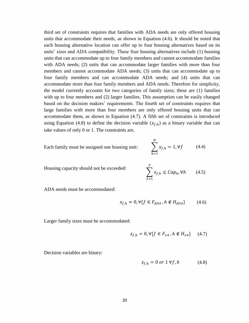
In order to ensure the practicality of the model, four sets of constraints are developed.

The first set of constraints requires that each family is provided one housing unit, as

shown in Equation (4.4). The second set ensures that the capacity of each housing

alternative is not exceeded by over-allocating families, as shown in Equation (4.5). The

(4.3)

20

third set of constraints requires that families with ADA needs are only offered housing

units that accommodate their needs, as shown in Equation (4.6). It should be noted that

each housing alternative location can offer up to four housing alternatives based on its

units’ sizes and ADA compatibility. These four housing alternatives include (1) housing

units that can accommodate up to four family members and cannot accommodate families

with ADA needs; (2) units that can accommodate larger families with more than four

members and cannot accommodate ADA needs; (3) units that can accommodate up to

four family members and can accommodate ADA needs; and (4) units that can

accommodate more than four family members and ADA needs. Therefore for simplicity,

the model currently accounts for two categories of family sizes; these are (1) families

with up to four members and (2) larger families. This assumption can be easily changed

based on the decision makers’ requirements. The fourth set of constraints requires that

large families with more than four members are only offered housing units that can

accommodate them, as shown in Equation (4.7). A fifth set of constraints is introduced

using Equation (4.8) to define the decision variable ( ) as a binary variable that can

take values of only 0 or 1. The constraints are,

Each family must be assigned one housing unit:

Housing capacity should not be exceeded:

ADA needs must be accommodated:

Larger family sizes must be accommodated:

Decision variables are binary:

∑

(4.4)

∑

(4.5)

(4.6)

(4.7)

(4.8)

21

where,

= binary decision variable that defines whether family is assigned to housing

alternative or not;

= number of displaced families applying for temporary housing;

= number of available temporary housing alternatives;

= capacity of temporary housing alternative in number of available units;

= set of displaced families with ADA needs;

= set of available temporary housing alternatives that can accommodate ADA needs;

= set of displaced families with more than four family members; and

= set of available temporary housing alternatives that can accommodate families

with more than four family members.

4.2. Customized Hungarian Algorithm

This temporary housing optimization is a special case of a transportation problem. The

general transportation problem is concerned with distributing any commodity (housing

unit) from sources (housings) to destinations (families), in such a way as to minimize or

maximize the total distribution weight (cost). It takes advantage of total unimodularity of

its Constraint Coefficients Matrix and applies algorithms, such as the Hungarian

Algorithm, to achieve tremendous computational savings (these algorithms are

polynomial time solvable). Moreover, these algorithms can be easily implemented in the

weight (cost) table format which saves memory consumption significantly (Nemhauser

and Wolsey, 1988). Table 4.1 shows an example of a weight table, where is the

weight (cost) of transporting the unit item from th source to the th destination.

Destination

Source

1 2 …

1 …

2 …

… … … …

…

Table 4.1. Weight Table

Now in order to use the Hungarian Algorithm, one must transform the temporary housing

problem to the weight table format. In addition, each family in the problem can only

22

accept one housing unit, while the housings provide multiple housing units. To address

this issue and to be able to maximize the computational efficiencies by using the

Hungarian algorithm, a customized version of the Hungarian algorithm is developed. The

following subsections present (1) a customized formulation of the objective function to

be solvable using the Hungarian algorithm; (2) the newly developed variant of the

Hungarian algorithm; and (3) a case example to illustrate the advantage of the algorithm.

It should be noted that a description of the original formulation of the Hungarian

algorithm can be found at Schrijver (2003).

Modified Formulation of the Objective Function

To reformulate the temporary housing problem in a weight table, the weight ( ) for

each assignment needs to be defined. This weight should represent the contribution of

each assignment in the objective function formulated as Equation (4.3). The objective

function ( ) needs to be formulated as a function of the temporary housing decision

variables ( ) with the assignments weights ( ). First, OP can be formulated by

applying some algebra transformation to Equations (3.4) to (4.3). Accordingly, the new

formulation of OP is developed as shown in Equation (4.9),

Moreover, the assignments weights ( ) can be computed for each family and

housing alternative , as shown in Equation (4.10),

Table 4.2. Weight Table for Temporary Housing Problem

∑ ∑

[ (

)

]

(4.9)

( )

. (4.10)

Housing

Family …

…

…

… … … …

…

23

Table 4.2 shows the resulting weight table for this temporary housing problem.

Therefore, can be formulated as a function in and , as shown in Equation

(4.11),

Maximize:

It should be noted that since the term

in Equation (4.9)

is a constant, it can be omitted from the maximization function with no impact on the

generated optimal solutions.

Proposed Variant of Hungarian Algorithm

The Hungarian Algorithm handles constraints (4.4), (4.5) and (4.8), however, it cannot

easily incorporate constraints (4.6) and (4.7). For this reason, we move the constraints

into the objective function by setting the weights equal to negative infinity for the

appropriate and combinations identified in (4.6) and (4.7). And to better explain the

algorithm, the symbols used in this section are changed slightly from the previous part of

the thesis, the index for families is instead of , and the th family is denoted by ; the

index for housing is and the th housing is denoted by .

The Algorithm Procedures are explained as follow:

0. There are displaced families and housing alternatives . The housing

alternative has the number of housing units equal to . One housing unit can only

allow one family to live in it, and the housing units of all housings can guarantee every

family has a place to live, i.e., ∑ .

As discussed earlier, assigning family to housing alternative results in a benefit

equal to weight . The objective of problem is to maximize the overall benefit.

However, the algorithm is implemented for minimization, so the value of each weight is

redefined as , where the largest value among all weights. The

decision variables are denoted as where indicates that family is assigned to

housing , and means is not assigned to . During the implementation of the

∑ ∑

.

(4.11)

24

algorithm, can have the value of 2 to represent a special condition, but this will not

last to the end and affect the final results. The initial condition is that no family is

assigned to any housing, i.e., for all ; and all families and housings are

uncovered.

1. For each , identify the set of indices ( can have

several elements due to tied weight values), let be the smallest index in .

If ∑ , let .

2. For each , we say family is covered. If all the

families are covered, terminate the algorithm with the optimal solution. Otherwise, go to

Step 3.

3. For each , identify the set using the current

weights. Find the first pair such that , and both and are uncovered. If

there is no such pair, go to Step 6. If there is a pair , let If the number of

elements in the set { | } equals to , uncover all of the families

, and cover the housing , go back to the start of step 3. Otherwise, go to Step

4.

4. In order to create an assignment for an additional family and update prior assignments to

maintain feasibility, perform the following steps:

4.1. Let , , go to Step 4.2.

4.2. Find the index such that , if there is no such , go to step 4.4, otherwise, go to

Step 4.3.

4.3. Set , , and there must be a such that , Increment

again, and let . Then return to Step 4.2.

4.4. Build ordered list with all . Then for each , if , set

, and

if , set

( in the list), go to Step 5.

5. Uncover all families and housings, and for all the elements in { | } (not all

are used in the ordered list in Step 4), let them be zero again, go back to Step 2.

6. Find = . For every covered

family, we increase its weights by , for every uncovered housing, we decrease its

weights by . Then go back to Step 3.

25

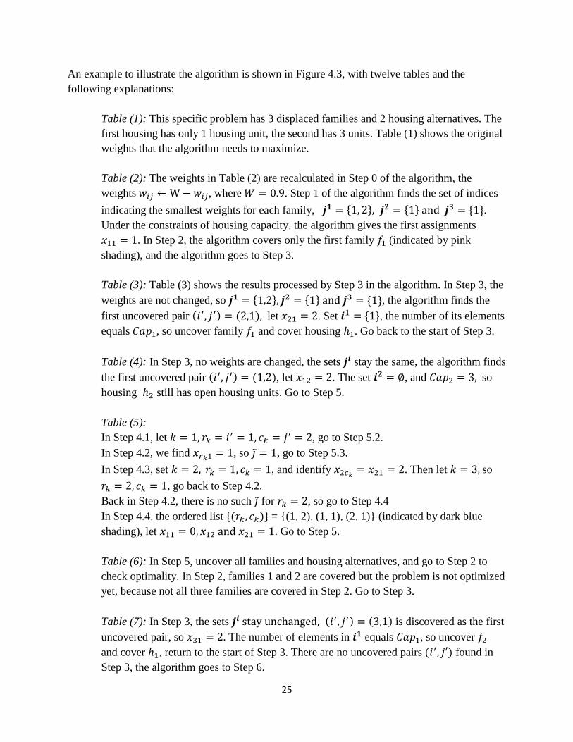
An example to illustrate the algorithm is shown in Figure 4.3, with twelve tables and the

following explanations:

Table (1): This specific problem has 3 displaced families and 2 housing alternatives. The

first housing has only 1 housing unit, the second has 3 units. Table (1) shows the original

weights that the algorithm needs to maximize.

Table (2): The weights in Table (2) are recalculated in Step 0 of the algorithm, the

weights , where . Step 1 of the algorithm finds the set of indices

indicating the smallest weights for each family, .

Under the constraints of housing capacity, the algorithm gives the first assignments

. In Step 2, the algorithm covers only the first family (indicated by pink

shading), and the algorithm goes to Step 3.

Table (3): Table (3) shows the results processed by Step 3 in the algorithm. In Step 3, the

weights are not changed, so , the algorithm finds the

first uncovered pair let . Set , the number of its elements

equals , so uncover family and cover housing . Go back to the start of Step 3.

Table (4): In Step 3, no weights are changed, the sets stay the same, the algorithm finds

the first uncovered pair , let . The set , and so

housing still has open housing units. Go to Step 5.

Table (5):

In Step 4.1, let , go to Step 5.2.

In Step 4.2, we find , so , go to Step 5.3.

In Step 4.3, set , and identify . Then let so

, go back to Step 4.2.

Back in Step 4.2, there is no such for , so go to Step 4.4

In Step 4.4, the ordered list = {(1, 2), (1, 1), (2, 1)} (indicated by dark blue

shading), let . Go to Step 5.

Table (6): In Step 5, uncover all families and housing alternatives, and go to Step 2 to

check optimality. In Step 2, families 1 and 2 are covered but the problem is not optimized

yet, because not all three families are covered in Step 2. Go to Step 3.

Table (7): In Step 3, the sets is discovered as the first

uncovered pair, so The number of elements in equals , so uncover

and cover , return to the start of Step 3. There are no uncovered pairs found in

Step 3, the algorithm goes to Step 6.

26

Table (8): In Step 6, the smallest uncovered weight is (indicated by dark green

shading), so

Table (9): The weights of all covered families are increased by 0.2, the weights of all

uncovered housings are decreased by 0.2. Go back to Step 3.

Table (10): In Step 3, using the current weights, the sets are updated to

is the first uncovered pair, and , its number of

elements is less than , so still has open housing units. Go to Step 4.

Table (11):

In Step 4.1, let , go to Step 4.2.

In Step 4.2, we find , so , go to Step 4.3.

In Step 4.3, set , and identify . Then let so

, go back to Step 4.2.

In Step 4.2, there is no such for , then go to Step 4.4

In Step 4.4, the ordered list = {(2, 2), (2, 1), (3, 1)} (indicated by dark blue

shading), let . Go to step 6.

Table (12): In Step 6, uncover all families and housing alternatives and go to Step 2 to

check optimality. In Step 2, we cover families 1, 2, and 3, and since all the families are

covered, terminate the algorithm. The solution is

. The overall weight of the original problem is

.

The example illustrates how the algorithm obtaining an optimal solution. To explore

other solutions on the Pareto-optimal front, the user would modify and and

calculate the weights according to Equation (4.10).

27

Figure 4.3. Algorithm Case Example

28

Case Example

This subsection presents an application example in order to demonstrate the big

computational and memory savings associated with the proposed implementation. The

following parts briefly describe the application example input data, compare the

optimization results obtained using each of the traditional Branch and Bound algorithm

and the customized Hungarian algorithm, and discuss the computational performance.

Moreover, the last part of this subsection demonstrates the generation of Pareto optimal

solutions.

The purpose of this application example is to represent the optimization of a large-scale

temporary housing optimization problem. To this end, this application example utilized

the collected data for the temporary housing case study presented by El-Anwar et al.

(2008). The case study involved simulating the reoccurrence of the 1994 Northridge

earthquake using HAZUS®-MH V1.1. This simulation generated the expected

distribution of displaced families in Los Angeles County, CA by census tracts. In this

application example, 5,000 of those families were assumed to be in need of temporary

housing. The socioeconomic needs of those families were randomly generated within

practical ranges. Furthermore, housing data were obtained from the database of available

temporary housing alternatives generated for the aforementioned Northridge earthquake

case study. This data was generated using a detailed online search of available temporary

housing alternatives in Los Angeles County. These alternatives consist of campsites for

travel trailers, hotels, inns, motels, as well as other lodges. A total of 178 housing

alternatives from this database were included in this application example with a total

capacity of 34,768 housing units. This database also provided other needed data about

these housing alternatives, such as their addresses, housing capacities, time availability,

housing quality rating, neighborhood safety, area unemployment rate, and access to

public services and transportation. Moreover, the authors complemented this data by

identifying samples of the available services within the cities of these housing

alternatives, such as public K-12 schools and healthcare facilities. Any other needed data

for running the model was reasonably assumed.

Using the aforementioned data, a pool of 5,000 displaced families and 178 temporary

housing alternatives is created. This pool was used to develop 13 temporary housing

problems ranging in size from small-scale problems (e.g., housing 500 families and 15

housing alternatives) to large-scale problems (e.g., housing 5,000 families and 178

housing alternatives), as shown in Table 4.3. These 13 problems are ordered based on

their computational complexity as a function in the number of decision variables, which

29

is equal to the number of displaced families (F) multiplied by the number of available

housing alternatives (H).

Problem

#

Number

of

Families

( )

Number of

Housing

alternatives

( )

Number of

Decision

Variables

( )

Running Time(s)

Customized

Hungarian

Branch & Bound

1 500 15 7,500 0.016 15

2 500 30 15,000 0.006 104

3 600 30 18,000 0.047 129

4 500 40 20,000 0.006 305

5 700 30 21,000 0.101 328

6 800 30 24,000 0.154 Out of Memory

7 500 50 25,000 0.178 Out of Memory

8 1000 30 30,000 0.269 Out of Memory

9 1000 60 60,000 1.83 Out of Memory

10 2000 60 120,000 20.0 Out of Memory

11 2000 120 240,000 46.0 Out of Memory

12 4000 120 480,000 461.0 Out of Memory

13 5000 178 890,000 1,534.0 Out of Memory

Table 4.3. Algorithm Performance

The Branch and Bound algorithm and customized Hungarian algorithm were run on a 2.8

GHz Intel Pentium D processor with 3 GB of random access memory and a 64-bit

operating system using MATLAB®. The Branch and Bound algorithm used the

“bintprog” function from the MATLAB® Optimization Toolbox. The customized

Hungarian algorithm follows the procedure explained in the last section (See the

Appendix for the MATLAB code “Hungarian_Housing.m”), and the code is modified

from the original Hungarian algorithm written by Melin (2006). Table 4.3 shows the

computational efficiency for the 13 temporary housing problems using the two

implementations. The customized Hungarian algorithm outperforms a general Branch and

Bound algorithm in this problem.

In order to demonstrate the proposed model’s capabilities in identifying the optimal

tradeoffs between maximizing socioeconomic welfare and minimizing total costs, the

customized Hungarian algorithm is applied to the full scale problem. This problem

includes optimizing temporary housing assignments for 5,000 families with 178 housing

alternatives, resulting in 890,000 decision variables (5,000 178). In order to identify the

Pareto solutions that represent those optimal tradeoffs, different combinations of relative

weights should be assigned to and . To this end, the full scale housing problem

was solved for four combinations of weights; (1,0), (0.75, 0.25), (0.5, 0.5), and (0,1).

30

Table 4.4 shows the Pareto-optimal solutions for the ( ) weight combination as

well as the Utopia and Nadir points with the associated function values of .

The points are graphed in Figure 4.4. The tradeoffs for the objective functions are easily

interpreted. These results show that only four combinations of weights were enough to

draw a relatively accurate Pareto front for this case. The weight combinations of (0.75,

0.25) and (0.5, 0.5) could generate optimal solutions that are very close to the Utopia

point. The values of 89.8% and 90.9% are very close to the Utopia values of 92.2%.

And the values of 6,802 and 7,163 are very close to the Utopia value of 6,666.

The results inform a decision maker about the relative weights ( ) that are good

values to implement in the systems, and provide a range on the total monthly cost to

anticipate. The detailed assignments can also be compared to explore which housing

alternatives are likely to be filled to capacity.

Time (s) OSI TC( 1,000 USD)

(1, 0) 1533.728 92.2% 12,261

(0.75, 0.25) 2620.837 90.9% 7,163

(0.5, 0.5) 3221.85 89.8% 6,802

(0, 1) 1099.436 67.0% 6,666

Utopia Point 92.2% 6,666

Nadir Point 67.0% 12,261

Table 4.4 Optimization Results

Figure 4.4. Pareto Optimal Solution

31

V. DECISION SUPPORT MODULE

This chapter introduces two tools to support Emergency Management Agency in

decision making. The cost-socioeconomic tradeoff tool allows the Emergency

Management Agency to look at the total cost and overall family socio-economic

benefit among different Pareto-optimal solutions. The potential housing cost-benefit

analysis tool gives the agency the capability to virtually add potential housing

alternatives in the system, and test whether the housing alternatives benefit families in

an acceptable cost. The general structure of this module is shown in Figure 5.1.

Figure 5.1. General Structure of Module 4

5.1. Cost-Socioeconomic Tradeoff

As discussed in the last chapter, the Optimization module provides a set of Pareto

solutions. The Cost-Socioeconomic Tradeoff tool first displays all the solution in a

scatter graph, such as Figure 4.4, but without the Nadir and Utopia Points. Figure 5.2

illustrates the Pareto-optimal front, contrasting the Overall Socio-economic Index

versus the Monthly Total Cost. When clicking on any solution, the Tradeoff tool can

show the detail number of both objectives to help Emergency Management Agency to

evaluate the trade-off and make the final selection.

32

Figure 5.2. Cost-Benefit Analysis

5.2. Cost-Benefit Analysis for Potential Housing

In many cases, the Emergency Management Agency likes to see if it is worthwhile

that, by adding a potential housing alternative, the overall performance of the new

assignments will be improved. As shown in Figure 5.3, the potential housings can be

trailer homes, constructed temporary housing or military buildings, all of which

requires substantial cost to set them up. The Potential Housing Analysis function

allows Emergency Management Agencies to virtually add the potential housing in the

system, put estimated costs associated with it and go back to the optimization,

checking whether the housing fulfills families’ needs. The system will not directly

suggest a potential housing. Instead, it shows how many families will be assigned to

this potential housing if it is built, leaving Emergency Management Agency to make

the decision.

33

Figure 5.3. Potential Housing Analysis

(three different types of potential housing alternatives are added to the system)

VI. OUTPUT REPORTING MODULE

This chapter presents the last module of the system, the output reporting. After the

solution is selected by the Emergency Management Agency, the information is

automatically generated for different users. Once they re-log into their portals, the

results/assignments are available. Families have the right to refuse the offer and look

for their own housings. The system will collect their feedback and put the refused

housing unit back into the housing pool for later assignments.

34

Families’ Output Portal

Figure 6.1. Families’ Output Portal

As shown in Figure 6.1, when a family re-logs into the system, the portal will

generate one marker in the center, which indicates the location of the housing that has

been assigned to them. Google Map can provide the street view of the location, so

without visiting, the family can have a general idea of what the building looks like. In

addition, by clicking the marker, an information window will pop up: it tells the room

type, neighborhood safety, access to public transportation, unemployment rate, etc.

At the end of the information window, the family needs to decide whether to accept

this offer. If family decides to refuse the offer, the information window will become a

comment board; the family can leave the reason why this housing unit does not fulfill

its socioeconomic needs. All the messages are stored in the database for developers

and Emergency Management Agency to improve the system.

Housing Providers’ Output Portal

The Output Portal for a Housing Provider contains the list of families that will live in

its housing units. The information only includes each family’s id. Figure 5.2 presents

the assignment table for housing #62. Once a family in the list turned down the offer,

the family will be automatically erased from the list.

35

Figure 6.2. Family List for Housing Provider #62

Emergency Management Agency’s Output Portal

The Output Portal for Emergency Management Agency is designed in a database

browser like format. The Emergency Management Agency can use queries to view

different information on the assignment table. He can request for a specific family’s

housing assignment or check the list of families assigned in a motel. Some sample

reports are shown in Figure 6.3.

Figure 6.3. Output Tables for Emergency Management Agency

36

VII. CONCLUSIONS

Current post-disaster temporary housing programs have limited capability to fulfill

the unique family’s socioeconomic needs. The inadequate strategic planning and lack

of decision support tools increasingly resulted in issues such as high overall cost, late

delivery and frequent family complaints. This thesis presented a new web-based Post

Disaster Temporary Housing Management system to transform the current inefficient

practice. Its new framework effectively collects families’ specific socioeconomic

needs, leverages available housing stock in impacted areas, matches housing offerings

to displaced families specific needs, maximizes the cost effectiveness of temporary

housing plans, provides support tools to decision makers and automates the process of

housing services procurement. Accordingly, the main contribution of this thesis is to

transform the current practice of post disaster temporary planning and execution.

Furthermore, some of the developed tools and methodologies can also be applied to

other fields.

The system aims at achieving two main objectives: (1) matching families’

socioeconomic needs to the characteristics and location of each housing alternative;

and (2) minimizing the life cycle costs of temporary housing. The implementation of

the system adopts a comprehensive methodology that consists of five main modules,

including (1) Data Acquisition Module; (2) Data Analysis Module; (3) Multi-

Objective Optimization Module; (4) Decision Support Module; and (5) Output

reporting Module. The first two modules are capable of providing customized

temporary housing assistance tailored to the specific social, economic, and

psychological needs of displaced families as compared to the one-size-fits-all current

approach. The multi-objective optimization was implemented using a customized

Hungarian Algorithm. It is proposed because of its effectiveness in identifying

Pareto-optimal solutions and the efficiency of its computational requirements. Two

decision support tools leverage available housing stock following disasters and

conduct cost-benefit analysis on the provision of other temporary housing forms such

as travel trailers and mobile homes.

This thesis has resulted in three peer-evaluated journal articles, one of which has been

accepted in the ASCE Journal of Construction Engineering and Management, and the

other two are still under review for publication. Further investigations are currently

underway to identify methods that are capable of capturing and improving displaced

families satisfaction with offered housing units as well as methods of enabling the

automation of a negotiation scheme between emergency management agencies and

housing providers. The final product will also include a special interface for mobile

devices such as smart phones.

37

Bibliography

Bolin, R. (1982). “Long-term family recovery from disaster.” Institute of Behavioral

Science Monograph 36, University of Colorado, Boulder.

Bolin, R. (1993). ‘‘Post-earthquake shelter and housing: Research findings and policy

implications.’’ 1993 National Earthquake Conference Monograph 5: Socioeconomic

Impacts, Committee on Socioeconomic Impacts, ed., Central United States Earthquake

Consortium, Memphis, Tenn., 107–131.

Bolin, R. C. and Bolton, P. (1986). Race, religion, and ethnicity in disaster recovery,

Boulder, CO: Institute of Behavioral Science, University of Colorado.

Comerio, M. C. (1997). “Housing repair and reconstruction after Loma Prieta.” National

Information Service for Earthquake Engineering, University of California Berkeley, 1997,

http://nisee.berkeley.edu/loma_prieta/comerio.html.

Comerio, M. C. (1998). Disaster Hits Home: New Policy for Urban Housing Recovery.

Berkeley: University of California Press, Berkeley, CA.

Deb, K., Agrawal, S., Pratap, A., and Meyarivan, T. (2001). “A Fast Elitist Non-

Dominated Sorting Genetic Algorithm for Multi-objective Optimization,” KANGAL

Report 200001, Genetic Algorithm Laboratory, Indian Institute of Technology, Kanpur,

India.

El-Anwar, O. (2009) “MULTI-OBJECTIVE OPTIMIZATION FOR TEMPORARY

HOUSING ARRANGEMENTS AFTER NATURAL DISASTERS”, Doctoral

Dissertation, University of Illinois at Urbana-Champaign.

El-Anwar, O. and Chen, L. (2012) (a) “Computing a Displacement Distance Equivalent

to Support Planning for Post-Disaster Temporary Housing Projects,” Journal of

Construction Engineering and Management, ASCE, accepted.

El-Anwar, O. and Chen, L. (2012) (b) “Maximizing the Computational Efficiency of

Temporary Housing Decision Support following Disasters,” Journal of Computing in

Civil Engineering, ASCE, in review.

38

El-Anwar, O. and Chen, L. (2012) (c) “Customized Development of Temporary Housing

Projects to Meet Displaced Populations Needs,” Journal of Urban Planning and

Development, ASCE, in review.

El-Anwar, O. and K. El-Rayes (2007). “Post-Disaster Optimization of Temporary

Housing Efforts,” Proc., ASCE Construction Research Congress, Island of Grand

Bahamas. 6–8 May.

El-Anwar, O., El-Rayes, K., and Elnashai, A. (2008). “Multi-Objective Optimization of

Temporary Housing for the 1994 Northridge Earthquake.” Journal of Earthquake

Engineering, 12(1), 81- 91.

El-Anwar, O., El-Rayes, K., and Elnashai, A. (2009) (a). “An Automated System for

Optimizing Post-Disaster Temporary Housing Allocation,” Journal of Automation in

Construction, 18(7), 983-993.

El-Anwar, O., El-Rayes, K., and Elnashai, A. (2009) (b). “Optimizing Large-Scale

Temporary Housing Arrangements after Natural Disasters,” Journal of Computing in

Civil Engineering, ASCE, 23(2), 110 - 118.

El-Anwar, O., El-Rayes, K., and Elnashai, A. (2010) (a). “Maximizing Temporary

Housing Safety after Natural Disasters,” Journal of Infrastructure Systems, ASCE, 16(2),

138-148.

El-Anwar, O., El-Rayes, K., and Elnashai, A. (2010) (b). “Maximizing the Sustainability

of Integrated Housing Recovery Efforts,” Journal of Construction Engineering and

Management, ASCE, 136(7), 794-802.

El-Anwar, O., El-Rayes, K., and Elnashai, A. (2010) (c). “Minimization of

Socioeconomic Disruption for Displaced Population Following Disasters,” Disasters,

34(3), 865−883.

Elnashai, A., Hampton, S., Karaman, H., Lee, J.S., McLaren, T., Myers, J., Navarro, C.,

Sahin, M., Spencer, B., and Tolbert, N. (2008) (a). “Overview and Applications of

MAEviz – HAZTURK 2007,” Journal of Earthquake Engineering, 12(1), 100 — 108.

Elnashai, A., Hampton, S., Lee, J.S., McLaren, T., Myers, J., Navarro, C., Spencer, B.,

and Tolbert, N. (2008) (b). “Architectural Overview of MAEviz – HAZTURK,” Journal

of Earthquake Engineering, 12(1), 92 — 99.

39

FEMA (2005) (a). “All Temporary Housing Options Being Considered,” Federal

Emergency Management Agency, Release number: 1603-004.

<http://www.fema.gov/news/newsrelease.fema?id=18820>, (December 18, 2011).

FEMA (2005) (b). “Disaster Recovery Officials Work to Get People Closer to Home,”

Federal Emergency Management Agency, Release number: 1604-074.

<http://www.fema.gov/news/newsrelease.fema?id=19781>, (December 18, 2011).

FEMA (2005) (c). “Programmatic environmental assessment: Temporary housing for

disaster victims of Hurricane Katrina.” FEMA-DR-1604-MS, September 2005.

FEMA (2006). “Alternative Housing Pilot Program - Guidance and Application Kit,”

Department of Homeland Security, Federal Emergency Management Agency, September

15, 2006 <http://www.fema.gov/pdf/government/grant/ahpp_guidance.pdf>, (October 27,

2008).

FEMA (2007). “Emergency Temporary Group Housing Site Selection Guidelines:

Minimizing Environmental/Historic/Safety Problems,” Federal Emergency Management

Agency, FEMA HQ Regions 4 and 6.

<http://www.fema.gov/pdf/plan/ehp/thsiteselection.pdf>, (December 18, 2011).

Friday, B. E. (1999). “Rebuilding shelter after natural disasters: Three decades of USAID

experience in Latin America and the Caribbean.” Prepared for United States Agency for

International Development, Contract No. PCE-I-00-96-00008-00, Delivery Order

Number 3, PADCO, Inc.

Golec, J. (1983). “A contextual approach to the social psychological study of disaster

recovery,” Journal of Mass Emergencies and Disasters, 1, August, 255-276.

Hidayat, B and Egbu, C (2010). “A literature review of the role of project management in

post-disaster reconstruction,” In: Egbu, C. (Ed), Proc., 26th Annual ARCOM Conference,

6-8 September 2010, Leeds, UK, Association of Researchers in Construction

Management, 1269-1278.

Johnson, C. (2002) (a) "Planning consideration for temporary accommodation after

disasters: An example of the 1999 Turkish earthquake.” Proc., i-Rec Conference on

Improving Post-Disaster Reconstruction in Developing Countries, University of Montreal,

Montreal, Canada, 23-25 May, 2002.

40

Johnson, C. (2002) (b) “What's the big deal about temporary housing? Types of

temporary accommodation after disasters: An example of the 1999 Turkish earthquake.”

Proc., TIEMS 2002 International Disaster Management Conference, University of

Waterloo, 14-17 May, 2002. TIEMS, Canada.

Johnson, C. (2007). “Impacts of prefabricated temporary housing after disasters: 1999

earthquakes in Turkey.” Habitat International, 31(1), 36-52.

Kruglanski, A. W. and Icek A. (1983). “Bias and Error In Human Judgment.” European

Journal of Social Psychology 13, 1-44.

Kandil, A., El-Rayes, K., and El-Anwar, O. (2010). "Optimization Research: Enhancing

Robustness of Large-Scale Multi-Objective Optimization in Construction," Journal of

Construction Engineering and Management, ASCE, 136(1), 17-25.

Lizarralde, G. and Johnson, C. (2003). “Houses of candied sugar: Comparative research

on controversial temporary housing after earthquake disasters in Colombia and Turkey.”

Proc., International Association for Housing Science World Congress on Housing

Process and Product, Montreal, Canada, 23–27 June, 2003. Montreal: IAHS.

Melin, A. (2006). “Hungarian Algorithm.” Matlab File Exchange.

<http://www.mathworks.com/matlabcentral/fileexchange/11609-hungarian-

algorithm/content/Hungarian.m>.

MAEviz (2008). “MAEviz Software.” Mid-America Earthquake Center.

<http://mae.ce.uiuc.edu/software_and_tools/maeviz.html>, (Febraury 12, 2008).

McLaren, T., Myers, J., Lee, J.S., Tolbert, N., Hampton, S., and Navarro, C. (2008).

“MAEviz: An Earthquake Risk Assessment System.” Proc. of the 16th ACM

SIGSPATIAL International Conference on Advances in Geographic Information Systems,

Irvine, California.

McLaren, T., Navarro, C., Lee, J.S., Hampton, S., Tolbert, N., Spencer, B.F., and

Elnashai, A. (2009). “Coupling Network Analysis using MAEviz Building Blocks.” Proc.

of 2009 NSF Engineering Research and Innovation Conference, Honolulu, Hawaii.

Newhauser, G. and Wolsey, L. (1988). “Integer and Combinatorial Optimization”, Wiley,

New York.

41

Quercia, R. G. and Bates, L. K. (2002). “The Neglect of America’s Housing:

Consequences and Policy Responses,” Working Paper 2002-02. Center for Urban and

Regional Studies, The University of North Carolina at Chapel Hill.

Rakes, T., Fetter, G., Deane, J., and Rees, L. (2010). “An assignment model for the

interim housing of disaster victims,” Proc., 2010 Southeast Decision Sciences Institute

Conference, Wilmington, NC, 2010.

Saaty, T. L. (1980). The analytic hierarchy process, McGraw-Hill, New York.

Schrijver, A. (2003). Combinatorial optimization, Polyhedra and Efficiency, Springer,

Verlag, Germany.

Shlay, A. B. (1995) “Housing in the Broader Context in the U.S." Housing Policy Debate,

6(3).

Sinnott, R.W. (1984). “Virtues of the Haversine,” Sky and Telescope, 68(2), p. 159.

Tomioka, T. (1997). “Housing Reconstruction Measures from the Great Hanshin-Awaji

Earthquake.” In Proceedings of the 5th United States/Japan Workshop on Earthquake

Hazard Reduction, Pasdena, California, January 15–17, 1997 (pp. 37–57). Oakland:

Earthquake Engineering Research Institute.

White, J. A., Case, K. E., Pratt, D. B., and Agee, M. H. (1998). “Comparison of

alternatives.” Principles of engineering economic analysis, fourth edition, John Wiley and

Sons, Inc., 143-255.

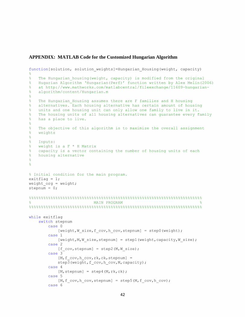
42

APPENDIX: MATLAB Code for the Customized Hungarian Algorithm

function[solution, solution_weights]=Hungarian_Housing(weight, capacity) % % The Hungarian_housing(weight, capacity) is modified from the original % Hugarian Algorithm ‘Hungarian(Perf)’ function written by Alex Melin(2006) % at http://www.mathworks.com/matlabcentral/fileexchange/11609-hungarian- % algorithm/content/Hungarian.m % % The Hungarian_Housing assumes there are F families and H housing % alternatives. Each housing alternative has certain amount of housing % units and one housing unit can only allow one family to live in it. % The housing units of all housing alternatives can guarantee every family % has a place to live. % % The objective of this algorithm is to maximize the overall assignment % weights % % Inputs: % weight is a F * H Matrix % capacity is a vector containing the number of housing units of each % housing alternative % %

% Initial condition for the main program. exitflag = 1; weight_org = weight; stepnum = 0;

%%%%%%%%%%%%%%%%%%%%%%%%%%%%%%%%%%%%%%%%%%%%%%%%%%%%%%%%%%%%%%%%%%%%%%%% % MAIN PROGRAM % %%%%%%%%%%%%%%%%%%%%%%%%%%%%%%%%%%%%%%%%%%%%%%%%%%%%%%%%%%%%%%%%%%%%%%%%

while exitflag switch stepnum case 0 [weight,W_size,f_cov,h_cov,stepnum] = step0(weight); case 1 [weight,M,W_size,stepnum] = step1(weight,capacity,W_size); case 2 [f_cov,stepnum] = step2(M,W_size); case 3

[M,f_cov,h_cov,rk,ck,stepnum] =

step3(weight,f_cov,h_cov,M,capacity); case 4 [M,stepnum] = step4(M,rk,ck); case 5 [M,f_cov,h_cov,stepnum] = step5(M,f_cov,h_cov); case 6

43

[weight,stepnum] = step6(weight,f_cov,h_cov); case 7 % Algorithm Terminated with OPtimal Solution exitflag = 0; end end

% Calculate the sum of the assignment weights using the optimal solution solution = M; solution_weights=sum(sum(weight_org(solution==1)));

%%%%%%%%%%%%%%%%%%%%%%%%%%%%%%%%%%%%%%%%%%%%%%%%%%%%%%%%%%%%%%%%%%%%%%%% % Step 0: Setup the initial condition for the algorithm % %%%%%%%%%%%%%%%%%%%%%%%%%%%%%%%%%%%%%%%%%%%%%%%%%%%%%%%%%%%%%%%%%%%%%%%%

function [weight,W_size,f_cov,h_cov,stepnum] = step0(weight)

% The algorithm is implemented for minimization, weight = max(max(weight)) - weight; W_size = size(weight);

% A vector that shows if a family is covered % f_cov[i] = 1 indicates the ith family is covered % Families are initailly uncovered. f_cov = zeros(W_size(1),1);

% A vector that shows if a housing alternative is covered % h_cov[j] = capacity[j] indicates the jth housing alternative is covered % Housing alternatives are initially uncovered h_cov = zeros(W_size(2),1);

stepnum = 1;

%%%%%%%%%%%%%%%%%%%%%%%%%%%%%%%%%%%%%%%%%%%%%%%%%%%%%%%%%%%%%%%%%%%%%%%% % Step 1: Calculate the smallest weights for each family. % Build the first assignments under the Capacity Constraints %%%%%%%%%%%%%%%%%%%%%%%%%%%%%%%%%%%%%%%%%%%%%%%%%%%%%%%%%%%%%%%%%%%%%%%%

function [weight,M,W_size,stepnum] = step1(weight, capacity,W_size)

% Find the smallest weight for each family for i = 1:W_size(1) fmin = min(weight(i,:)); weight(i,:) = weight(i,:)-fmin; end

% Initialize the Assignment Matrix M = zeros(W_size);

temp_f_cov = zeros(W_size(1),1);

44

temp_h_cov = zeros(W_size(2),1);

% Build the first assignments under the capacity constraints for i = 1:W_size(1) for j = 1:W_size(2) if weight(i,j) == 0 && temp_f_cov(i) == 0 && temp_h_cov(j) <

capacity(j) M(i,j) = 1; temp_f_cov(i) = 1; temp_h_cov(j) = temp_h_cov(j)+1; end end end

stepnum = 2;

%%%%%%%%%%%%%%%%%%%%%%%%%%%%%%%%%%%%%%%%%%%%%%%%%%%%%%%%%%%%%%%%%%%%%%%% % Step 2: Cover the families that has assignments, if all families are % covered, terminate the algorithm with the optimal solution %%%%%%%%%%%%%%%%%%%%%%%%%%%%%%%%%%%%%%%%%%%%%%%%%%%%%%%%%%%%%%%%%%%%%%%%

function [f_cov,stepnum] = step2(M, W_size)

f_cov = sum(M,2); if sum(f_cov) == W_size(1) stepnum = 7; else stepnum = 3; end

%%%%%%%%%%%%%%%%%%%%%%%%%%%%%%%%%%%%%%%%%%%%%%%%%%%%%%%%%%%%%%%%%%%%%%%% % Step 3: Find the uncovered smallest weights for the families, change % the covers to cover all the smallest weights with mininum % number of covers. % %%%%%%%%%%%%%%%%%%%%%%%%%%%%%%%%%%%%%%%%%%%%%%%%%%%%%%%%%%%%%%%%%%%%%%%%

function [M,f_cov,h_cov,rk,ck,stepnum] = step3(weight,f_cov,h_cov,M,capacity)

W_size=size(weight); zflag = 1;

while zflag

% The row and cololumn index of the first uncovered smallest weight row = 0; col = 0; exitflag = 0;

% Find the first uncovered smallest weight of a family for i = 1:W_size(1) for j= 1:W_size(2) if weight(i,j) == 0 && f_cov(i) == 0 && h_cov(j) == 0 row = i;

45

col = j; exitflag = 1; end if exitflag, break, end end if exitflag, break, end end

% If there's no uncovered smallest weight, go to step 6 if row == 0 stepnum = 6; zflag = 0; rk = 0; ck = 0; else % Mark the smallest weight in the Assignement Matrix M(row,col) = 2;

% Check if the housing alternative that the smallest uncovered weight % locates is covered if sum(M(:,col)==1) == capacity(col) % Cover the housing alternative h_cov(col) = 1; % Uncover the families assigned to this housing alternative f_cov(M(:,col)==1) = 0; else % The housing that has the uncovered smallest weight has % opening, go to step 4 to reallocate assignments start from % the family (rk) and housing alternative (ck) stepnum = 4; zflag = 0; rk = row; ck = col; end end end

%%%%%%%%%%%%%%%%%%%%%%%%%%%%%%%%%%%%%%%%%%%%%%%%%%%%%%%%%%%%%%%%%%%%%%%% % Step 4: Build the M-augmenting path (ordered list (rk, ck) ) % and increase the cardinality of the assignments by one %%%%%%%%%%%%%%%%%%%%%%%%%%%%%%%%%%%%%%%%%%%%%%%%%%%%%%%%%%%%%%%%%%%%%%%%

function [M,stepnum] = step4(M,rk,ck)

zflag = 1; k = 1; while zflag

% Find the housing that the family (rk) is assigned to cindex = find(M(rk(k),:)==1); if cindex > 0 k = k+1; ck(k,1) = cindex; rk(k,1) = rk(k-1);

46

else % If there is no assigned housing for this family, finish the path zflag = 0; end

if zflag == 1; % Find the family that has the smallest uncovered weight for the % housing (ck) rindex = find(M(:,ck(k))==2); k = k+1; ck(k,1) = ck(k-1); rk(k,1) = rindex; end end

% For the complete M-augmenting path, assign the families to the housings % not assigned to them on the path and unassign the families that assigned % to the housing on the path. for i = 1:length(ck) if M(rk(i),ck(i)) == 1 M(rk(i),ck(i)) = 0; else M(rk(i),ck(i)) = 1; end end

stepnum = 5;

%%%%%%%%%%%%%%%%%%%%%%%%%%%%%%%%%%%%%%%%%%%%%%%%%%%%%%%%%%%%%%%%%%%%%%%% % Step 5: Uncover the families and housing alternatives, unmark the % uncovered smallest weights that left from step 4 %%%%%%%%%%%%%%%%%%%%%%%%%%%%%%%%%%%%%%%%%%%%%%%%%%%%%%%%%%%%%%%%%%%%%%%%

function [M, f_cov, h_cov, stepnum] = step5(M, f_cov, h_cov)

f_cov = f_cov.*0; h_cov = h_cov.*0; M(M==2) = 0; stepnum = 2;

%%%%%%%%%%%%%%%%%%%%%%%%%%%%%%%%%%%%%%%%%%%%%%%%%%%%%%%%%%%%%%%%%%%%%%%% % Step 6: Find the smallest weight that is not covered, add it to all % the covered families, and deducted it from all the uncovered % housing alternatives. %%%%%%%%%%%%%%%%%%%%%%%%%%%%%%%%%%%%%%%%%%%%%%%%%%%%%%%%%%%%%%%%%%%%%%%%

function [weight,stepnum] = step6(weight,f_cov,h_cov)

minval = min(min(weight(f_cov == 0,h_cov ==0)));

weight((f_cov == 1),:) = weight((f_cov == 1),:) + minval;

47

weight(:,(h_cov == 0)) = weight(:,(h_cov == 0)) - minval;

stepnum = 3;

a web-based system for optimizing post disaster temporary

Documents