a wide range robust pss design based on power system pole-placement using linear matrix inequality

Journal of ELECTRICAL ENGINEERING, VOL. 63, NO. 4, 2012, 233–241

A WIDE RANGE ROBUST PSS DESIGN BASEDON POWER SYSTEM POLE–PLACEMENTUSING LINEAR MATRIX INEQUALITY

Mohammad Ataei — Rahmat-Allah Hooshmand— Moein Parastegari

∗

In this paper, a new method for robust PSS design based on the power system pole placement is presented. In thisstabilizer, a feedback gain matrix is used as a controller. The controller design is proposed by formulating the problem ofrobust stability in a Linear Matrix Inequality (LMI) form. Then, the feedback gain matrix is designed based on the desiredregion of the closed loop system poles. This stabilizer shifts the poles of the power system in different operational pointsinto the desired regions in s -plane, such that the response of the power system will have proper damping ratio in all theoperational points. The uncertainties of the power system parameters are also considered in this robust technique. Finally,in order to show the advantages of the proposed method in comparison with conventional PSS, some simulation results areprovided for a power system case study in different operational points.

K e y w o r d s: power system stabilizer (PSS), robust stability, linear matrix inequality (LMI) problem, pole placement

1 INTRODUCTION

The dynamic stability is one of the most importantproblems in the power system which can be studied byusing nonlinear model of the power system. The nonlin-ear model of the system includes a series of nonlinearcomplicated equations. These nonlinear equations can belinearized around each operating point, such that smallsignal model of the power system can be determined. TheHefferon-Philips model is one of these power system lin-ear models [1–19]. The studies on linear system show thatthe system response has not enough damping ratio andit might be unstable in some operating points [1–8]. Inorder to increase the damping of the power system re-sponse, classical controllers can be used which are usuallydesigned for an operating point. If a phase lead transferfunction is used in control mechanism, a conventional PSSis achieved [1–19]. Since the PSS is designed for one opera-tional point, it has good performance only in the designedoperating condition and it should be redesigned to achievegood performance in the other operational points. There-fore, the desired PSS should stabilize the power systemin all operational points; ie, it should be robust againstthe changes in the operational conditions.

Adaptive control [3] and robust control strategies [4–15] are two main methods for solving this problem inpower system which have been led to adaptive PSS androbust PSS designs respectively. Since in adaptive PSS,an identification mechanism is required to adapt the PSSparameters, the complexity of online controller compu-tations will increase [3]. In contrast, in the robust PSS,

a fixed controller for different operational points is de-signed [4–15] which makes it more convenient than adap-tive PSS.

In the field of robust PSS, different methods basedon the H∞ control theory [5–15] and the QuantitativeFeedback Theory (QFT) [4] can be used to design a ro-bust stabilizer, however, the QFT based robust PSS isless used because of difficulties due to its trial and er-ror nature [4]. On the other hand, H∞ based methodsmostly guarantee the system stability and dont ensureany other constraint on system response [9–14]. There-fore, H∞ method can be combined with other methodsto improve performance of the PSS [5–8]. Some of thesedesirable methods are combination of H∞ and H2 [5, 19]or combination of H∞ and Pole-Placement methods [6–7]. In these combined methods, the design problem canbe converted to a LMI problem, whose solving determinesthe stabilizer parameters [4–19].

One important issue in robust PSS design is theachievement of wide range of stability. However, thismatter has not been considered in some previous studies[8, 10, 16, 17]. Moreover, unlike the methods presented inreferences [12, 18], simplified model cannot be used forpower system simulations. In order to achieve desirablepower system response, closed loop poles should be placedin specific zone. Although in references [5, 19] combinedH∞ and H2 methods are used, but this zonal constraintis not considered. Therefore, an important goal of thispaper is to consider the above mentioned characteristicssimultaneously.

On the other hand, for designing robust PSS, usually arobust strategy is used to determine lead transfer function

∗ Department of Electrical Engineering, Faculty of Engineering, University of Isfahan, Isfahan, Iran Hezar-Jerib St., P. Code: 8174673441,Isfahan, Iran, [email protected], Hooshmand [email protected]

DOI: 10.2478/v10187-012-0033-7, ISSN 1335-3632 c© 2012 FEI STU

Brought to you by | University of St Andrews ScotlandAuthenticated

Download Date | 11/30/14 1:00 PM

234 M. Ataei — R. Hooshmand — M. Parastegari: A WIDE RANGE ROBUST PSS DESIGN BASED ON POWER SYSTEM . . .

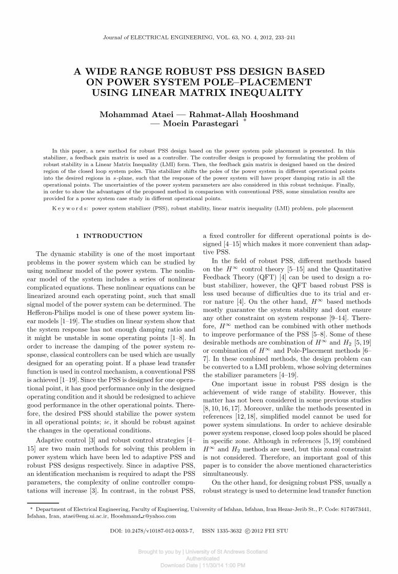
Fig. 1. Single machine infinite bus system Fig. 2. The linearized model of the synchronous generator in operatingpoint

parameters [5, 13], or feedback gains [7]. If a lead transferfunction is used as a controller, long settling time of powersystem response is achieved which is not desirable. In thisregard in references [5, 13], although the combined H∞

and pole placement methods has been used to achievewide range performance by solving LMI problem, butthey use lead transfer function which has caused longtransient response time.

Considering the above mentioned constraints, in thispaper desig of a robust PSS based on the power systempole placement is proposed in which a feedback gain ma-trix is used as a controller. For this purpose, combinedrobust and pole placement problem is formulated as aLMI problem whose by solving, the controller parame-ters are determined. Also in this method, parameter un-certainty is concluded in matrix elements by consideringhuge number of operational points. In addition, this prob-lem is solved such that wide range stability and shortsettling time is achieved simultaneously. Moreover, it canbe seen that power system remains stable in emergencycondition, i.e. in the operational points which is not con-sidered in range of usual operating points. In order toshow the advantages of the proposed method, some sim-ulation results are provided for a power system case studyin different operational points. It should be noted that forsolving the obtained LMI problem, the MATLAB pack-age is used and there are some numerical methods to solvethe LMI problem by MATLAB [21].

The remainder of this paper is organized as follows. InSection 2, the model of the power system with uncertaintyis studied. The LMI problem and its usage in robustcontrol design are reviewed in Section 3. In Section 4by combining robust power system stabilizer with poleplacement technique, an LMI problem is obtained. Theresults of applying the proposed approach to a powersystem is reported and analyzed in Section 5. Finally,some remarkable properties of the proposed method andconcluding remarks are explained in the last section.

2 THE POWER SYSTEM

MODEL WITH UNCERTAINTY

The power system is a nonlinear system; therefore to

study the small signal stability, the equations around each

operating point can be linearized. On the other hand,

when a single generator is connected to the infinite bus,

active power (P ), reactive power (Q) and transmission

line impedance between generator and infinite bus (Xe )

determine power system operating point. The power sys-

tem linearized model can be used to determine the sys-

tem eigenvalues. Fig. 1 shows a single line schematic dia-

gram of a single machine infinite bus system. The genera-

tor is fitted with an Automatic Voltage Regulator (AVR)

and a static excitation system. Neglecting the stator tran-

sients and the effect of damper windings, the generator

and exciter can be modeled as a 4th order system. This

power system with regulator and exciter linearized model

is named Hefferon Philips model which is shown in Fig.

2. In this figure, values of the K1 to K6 , KA , TA and

T ′do should be determined. The values of KA , TA and

T ′do are the synchronous generator parameters, which are

constant for each synchronous generator. On the other

hand, changes in the operating point (active power (P ),

reactive power (Q) and transmission line impedance be-

tween generator and infinite bus (Xe)) changes K1 to

K6 values. This model is a 4th order model, so it has 4

state variables. The state space equations of this model

are shown in the following equation.

x(t) = Ax(t) +Bu(t) , (1)

y = Cx(t) . (2)

where X(t) =[

∆δ(t) ∆ω(t) ∆E′q(t) ∆VF (t)

]⊤

is the state vector, y is the output signal, ∆ω(t) is se-

lected as the system output, and A is the state space



Journal of ELECTRICAL ENGINEERING 63, NO. 4, 2012 235

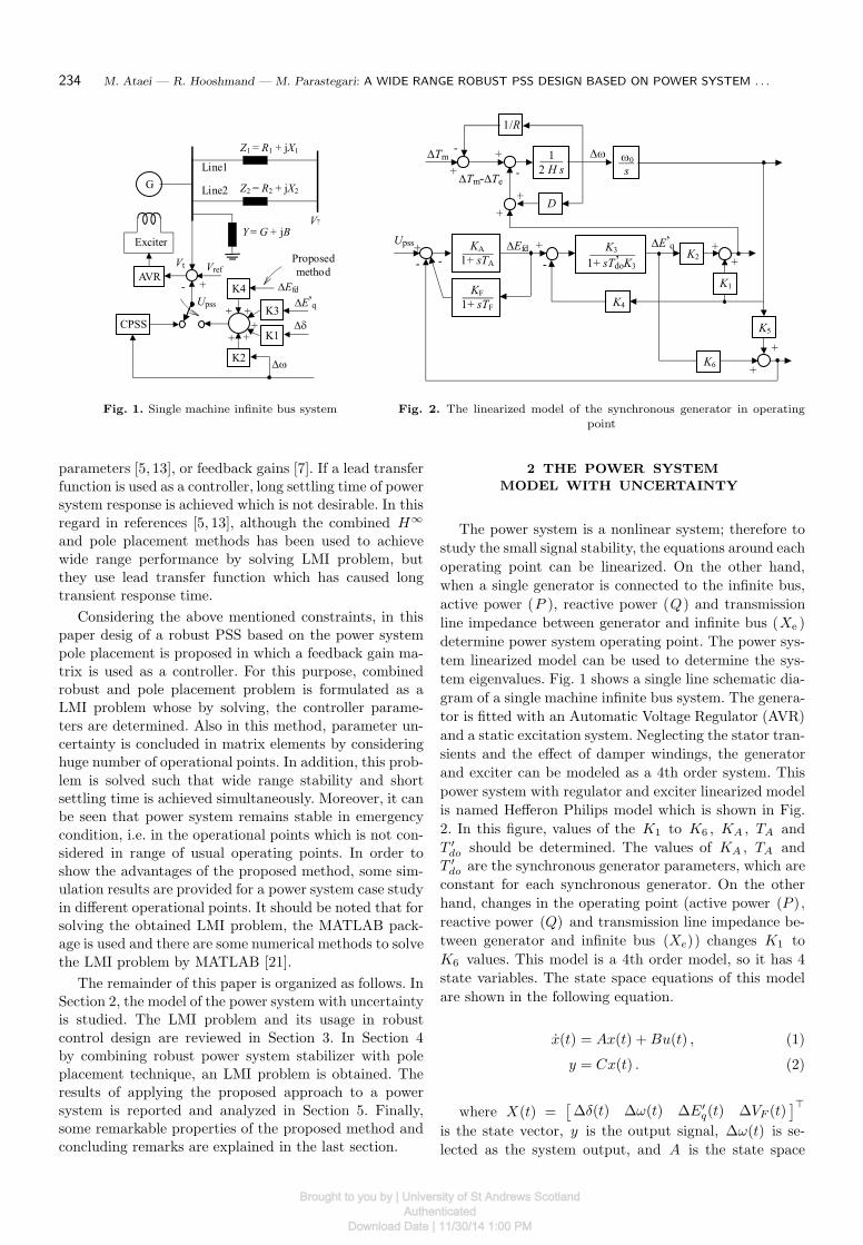
Fig. 3. Open loop poles (single machine system)

Fig. 4. D shape region for pole placemen

matrix where its elements are function of the loading con-ditions, B and C are

A =

0.0 2πf 0.0 0.0

−K1

M− D

M−K2

M0.0

− K4

T ′

do

0.0 − 1K1T

′

do

1T ′

do

−KAK5

TA0.0 −KAK6

TA− 1

TA

, (3)

B⊤ =[

0.0 0.0 0.0 KA

TA

]

, (4)

C = [ 0.0 1 0.0 0.0 ] . (5)

The under study system specifications are provided inAppendix A. The operating condition for this system iscompletely defined by the values of the real power, P ,the reactive power, Q , at the generator terminals andthe transmission line impedance, Xe . Values of P , Q andXe , are assumed to vary independently over the followingranges: 0.2 < Xe < 0.7 , −0.2 < Q < 0.5 , 0.4 < P <

1 . Changes in the operational point (P , Q and Xe ) leadsto changes in the elements of the A matrix and it leads tochanges in the linearized model eigenvalues. Fig. 3 showsthe open loop poles for this family of plants with P ,Q and Xe , varied over the specified range by steps of0.05. This step distance makes a set of operational pointswith 1900 different members, which contains most of theoperating conditions of the power system. Most of these

operational points don’t have adequate damping. So itis required to design a stabilizer which places the rotormode eigenvalues inside the acceptable region as is shownin Fig. 4.

3 LMI BASED ROBUST PSS DESIGN

In this section, after introducing some background ma-terials, describing the overall H∞ based state feedbackdesign with pole placement in terms of LMI problem [22]which is used in the proposed method in Section 4 is pre-sented.

3.1 Background Materials

This subsection discusses an LMI-based characteriza-tion for a wide class of pole clustering regions as well asan extended Lyapunov theorem for such regions. An in-teresting region for control purposes can be described bythe set S(α, r, θ) of complex numbers x+ jy such that

x < −α < 0 , |x+ jy| < r , x tan θ < −|y| . (6)

Locating the closed-loop poles of the system in this regionensures desired performance. Let D be a sub-region ofthe complex left-half plane. A dynamical system x = Ax

is called D -stable if all eigenvalues of the matrix A liein D .When D is the entire left-half plane, this notionreduces to asymptotic stability, which is characterized inLMI terms by the Lyapunov theorem, ie A is stable ifand only if there exists a symmetric matrix X satisfying

AX +XA⊤ < 0 , X > 0 . (7)

This Lyapunov characterization of stability has been ex-tended to a variety of regions [22]. These regions are poly-nomial regions of the following form

D ={

z ∈ C :∑

0≤k,l≤m

cklzkz−l < 0

}

(8)

where the coefficients ckl are real and satisfy ckl = clk .For polynomial regions, matrix A is D -stable if and onlyif there exists a symmetric matrix X such that

∑

k,l

cklAkX

(

A⊤)l< 0 , X > 0 . (9)

To have the ability of synthesizing the problem in theLMI framework, it is necessary to use conditions that areaffine in the state matrix A , such as the Lyapunov sta-bility condition (7). Moreover, defining the LMI regionsas follows is suitable for LMI-based synthesis. Hereafter,⊗ denotes the Kronecker product of matrices, and thenotation M = [µkl]1≤k,l≤m means that M is an m×m

matrix (block matrix) with generic entry (block) µkl .




Definition. A subset D of the complex plane is calledan LMI region if there exist a symmetric matrix α ∈[αkl] ∈ ℜm×m and a matrix β ∈ [βkl ∈ ℜm×m such that

D = {z ∈ C : fD(z) < 0} . (10)

fD(z) := α+ zβ + zβ⊤ = [αkl + βklz + βklz] . (11)

The pole location in a given LMI region can be charac-terized in terms of the following m×m block matrix

MD(A,X) := α⊗X + β ⊗ (AX) + β⊤(AX)⊤ =

[αklX + βklAX + βlkXA⊤]1≤k,l≤m . (12)

Theorem. The matrix A is D -stable if and only if there

exists a symmetric matrix X such that

MD(A,X) < 0 , X > 0 . (13)

Now, consider the region S(r, α, θ) as defined in (8)with α = r = 0. The eigenvalues of A lie in the sectorS(0, 0, θ) if and only if there exists a positive definitematrix P such that

(W ⊗A)P + P (W ⊗A)⊤ < 0 (14)

where W =

(

sin θ cos θ− cos θ sin θ

)

. On the other hand,

S(0, 0, θ) is an LMI region with characteristic function

fθ(z) =

(

sin θ(z + z) cos θ(z − z)− cos θ(z − z) sin θ(z + z)

)

. (15)

A has its poles in S(0, 0, θ) if and only if there existsX > 0 such that

(

sin θ(AX +AX⊤) cos θ(AX −AX⊤)

cos θ(XA⊤ −AX) sin θ(AX +AX⊤)

)

< 0 (16)

or equivalently

(W ⊗A)Diag(X,X) +Diag(X,X)(W ⊗A)⊤ < 0 . (17)

In comparison with relation (14), this last condition givesadditional information on the structure of P . It is alsomore suitable since the number of optimization variablesis divided by four when replacing P by Diag(X,X).

3.2 H∞ Based State-Feedback Design with Pole

Placement

This subsection discusses state-feedback synthesis withH∞ performance and pole assignment specifications.Here, the closed-loop poles are required to lie in someLMI region D contained in the left-half plane. Resultsare first derived in the nominal case and then extendedto uncertain systems.

Consider a linear time-invariant (LTI) system de-

scribed by

x(t) = Ax(t) +B1ω(t) ,

z∞(t) = C∞x(t) +D∞1ω(t)(18)

and let Tω z∞(s) denote the closed-loop transfer function

from ω to z∞ under state-feedback control u = kx . The

constrained H∞ problem is to find a state-feedback gain

K that:

• places the closed-loop poles in some LMI stability re-

gion D with characteristic function (11);

• guarantees the H∞ performance∥

∥Tω z∞

∥

∥

∞< γ .

Let (Acl, Bcl, Ccl∞, Dcl∞) denote realizations of Tω z∞ .

From mentioned theorem in Section 3.1 the pole-place-

ment constraint is satisfied if and only if there exists

XD > 0 such that

[

αklXD + βklAclXD + βlkXDA⊤cl

]

1≤k,l≤m< 0 . (19)

Meanwhile, the H∞ constraint is equivalent to the exis-

tence of a solution X∞ > 0 for the following LMI:

AclX∞ Bcl X∞C⊤cl∞

B⊤cl −I D⊤

cl∞

Ccl∞X∞ Dcl∞ −γ2I

< 0 . (20)

This result is known as the Bounded Real Lemma.

Our goal is to determine state feedback gains K that

satisfies the H∞ and pole constraints. From the previ-

ous discussion, this is equivalent to satisfy (19), (20).

While this problem is not jointly convex in the variables

(XD, X∞, Y,K), convexity can be enforced by finding a

common solution

X = XD = X∞ > 0 . (21)

Consequently LMI constraints can be summarized as the

following inequalities

[

αklX + βklU(X,L) + βlkU(X,L)⊤]

< 0 , (22)

U(X,L) + U(X,L)⊤ B1 V (X,L)⊤

B⊤1 −I D⊤

∞1

V (X,L) D∞1 −γ2I

< 0 (23)

U(X,L) := AX , V (X,L) := C∞X . (24)

In this stage, LMI optimization software such as the

MATLAB LMI Control Toolbox can be used to solve the

problem.




4 THE PROPOSED WIDE RANGE

ROBUST PSS BY USING LMI

4.1 Design Objectives

The Power system eigenvalues which show the relativestability of the system are determined by its linearizedmodel. These eigenvalues have not enough damping tostabilize power system response. It should be noted thatin power systems, a damping factor, ζ , of at least 10%and a real part, σ , not greater than −0.5 for the trou-blesome low frequency electromechanical mode, guaran-tees that the excited low frequency oscillations will dampdown in a reasonably short time. Such restriction on allthe system eigenvalues would imply that all the poles ofthe system lie in the left of the imaginary axis in a D

shape contour. This D shape contour is shown in Fig. 4.If a power system has above specifications, low frequencyoscillations will damp after a short time. However, a realpower system has not such a good structure and all ofits poles have not enough damping and might be un-stable. To stabilize the power system response, feedbackcontrollers are used. The feedback gains should be de-termined such that the closed loop eigenvalues shift tothe D shape region. These feedback gains should also besmall enough to prevent controllers saturation.

On the other hand, in this paper our goal is findingthe feedback gains such that it guarantees stable powersystem response in spite of changes in operational point.A robust controller and a well damped response is ob-tained in a wide range of operating points, if proposedmethod guarantees acceptable small signal transient inall operational points.

For this purpose, the robust controller design prob-lem is converted to a LMI problem. Thus, solving theLMI problem leads to robust power system stabilizer. Toaccomplish this, at first, system uncertainties should bestudied in the state space equations.

4.2 Representing the uncertainty in the power

system model

Dynamical behavior of a system can be described bystate space equations. These state space equations con-sist of power system parameters which are not constant.Therefore, the system should be determined by an uncer-tain state space model.

The state space equations of the uncertain system canbe considered as follows

Ex = Ax(t) +Bu(t) , (25)

y(t) = Cx(t) +Du(t) . (26)

where the matrices A , B , C , D , E depend on uncertainparameters which vary in some bounded sets. The matrixelements boundaries can be determined in n operatingpoints. Therefore changes in the operating point leads tochanges in the state space equations.

In the resultant, considering the uncertain elements

of each uncertain matrix, the matrices A and B can be

considered as the following form

(A,B) ∈

{

(

N∑

i=1

piAi ,

N∑

i=1

piBi

)

:

N∑

i=1

pi = 1 , pi ≥ 0

}

.

(27)

Such polytopic models may be resulted from convex inter-

polation of a set of models (A,B) identified in different

operating points. They also arise in connection with affine

parameter dependent models as

x = A(p)x +B(p)u . (28)

where p is a vector of real uncertain parameters and

A(p), B(p) are affine matrix-valued functions of p .

The uncertain matrix A of the under study power

system based on the presented model in Section 2 is as

follows

A =

0.0 a12 0.0 0.0a21 a22 a23 0.0a31 0.0 a33 a34a41 0.0 a43 a44

, (29)

The system matrix A(k) is affinely dependent on k , ie

A(k) can be rewritten in the following form

A0+a21A1+a23A2+a31A3+a33A4+a41A5+a43A6 (30)

where A0 , A1 , A2 , A3 , A5 and A6 are constant ma-

trices. Under different loading conditions each parameter

varies within a certain range as:

a21 ∈ [a−21, a+21] , a23 ∈ [a−23, a

+23] , a31 ∈ [a−31, a

+31] ,

a33 ∈ [a−33, a+33] , a41 ∈ [a−41, a

+41] and a43 ∈ [a−43, a

+43]

where a−ij and a+ij denotes the lower and upper bound

of the parameter aij respectively for all P ∈ [P−, P+] ,

Q ∈ [Q−, Q+] and xe ∈ [x−e , x

+e ] . These bounds can

be calculated using any standard optimization tech-

nique. This affine parameter-dependent model can be

converted to a polytopic model. The parameter vector[ a21 a23 a31 a33 a41 a43 ] ∈ ℜ6 takes values in a

parameter-box with 25 = 32 corners

kcor1 =[

a−21 a+23 a+31 a+33 a+41 a+43]⊤

,

kcor2 =[

a+21 a−23 a+31 a+33 a+41 a+43]⊤

,

...

kcor32 =[

a−21 a−23 a−31 a−33 a−41 a−43]⊤

.

(31)

Since A(k) is affine in k , it maps this parameter box to

a polytope of matrices with 32 vertices defined at each

parameter box corner.




4.3 Design Procedure

By considering above uncertainty description, feed-back gains should be determined such that the powersystem eigenvalues places in the desirable D region. Itshould be noted that an unnecessarily large shift of thesystem poles into the left half plane should be avoided,since this may lead to large feedback gains. Therefore,imposition of constraints enforces the closed loop polesto a D shape region specified with θ < 45◦ and −50 ≤σ ≤ −0.5. In the other word, the open loop poles of thewhole family of plants should be shifted to this region.

In Section 3 the issue of converting the state feedbackdesign to an LMI problem was discussed. These resultscan be extended for uncertain systems [22]. For brevity,in the following only converting the pole placement prob-lem by considering the uncertainty description of Sub-section 4.2 is discussed. Thus, solving the resultant LMIproblem leads to design of feedback gains, which is ro-bust against changes in the P,Q and Xe . Consequently,the power system eigenvalues are forced into the D shaperegion in the left half plane.

Consider the problem of computing a state feedbackgain K that forces the closed-loop eigenvalues into someLMI region D for all admissible values of A and B .The equation (25) is called quadratically D -stabilizableif there exists a gain K and a single Lyapunov matrixX > 0 such that MD(A+BK,X) < 0 for all admissiblevalues of A and B . In the continue, it is shown that thiscondition is also necessary, and the results are extendedto arbitrary LMI regions.

Let D be any LMI region, suppose that (25) isquadratically D -stabilizable with Lyapunov matrix X

and state-feedback gain K , and let L := KX . By con-sidering the condition MD(A+BK,X) < 0 at each vertex(Ai, Bi) of (27), the following necessary conditions on X ,L are achieved

[αklX + βkl(AiX +BiL) + βlk(AiX +BiL)⊤T ]k,l < 0

for i = 1, . . . , N , (32)

X > 0 . (33)

Conversely, it can be seen that any solution (L,X) of thisLMI system satisfies MD(A+BK,X) < 0 when formingthe weighted sum of the LMIs (32) with nonnegative coef-ficients p1, . . . , pN . Hence, the relations (32) and (33) arenecessary and sufficient for quadratic D -stabilizability.Note that LMI conditions for quadratic H∞ performanceover (27) are obtained similarly by writing (22), (23) ateach vertex of the polytopic plant.

Now, it is proposed to apply a full state feedbackcontroller using the described LMI based approach forachieving the robust D-stability requirement. Each stateis measured, multiplied by the appropriate gain and thensummed up before being fed at the reference input of theAutomatic Voltage Regulator. In a practical implemen-tation, additional hardware would be required for statemeasurements. For the 4th order model used here, the

states are the deviations in the load angle δ , rotor speedω , field voltage Efd and the internal voltage E′

q . The

values of δ , ω and Efd can be directly measured us-ing appropriate transducers. The internal voltage E′

q can

be computed from the instantaneous values of the statorcurrents and the equivalent circuit parameters. A poly-topic system is obtained for this set by choosing the A

and B matrices corresponding to the external values ofP , Q and Xe as stated in Subsection 4.2. All possiblecombinations of the minimum and maximum values ofeach of these 3 parameters are taken to generate a setof 8 vertex systems corresponding to the 8 corners of acube in the space with P , Q and Xe coordinates. Sincethe point with minimum Q and maximum P and Xe ,did not have a steady state load flow solution, it was re-placed by a nearby feasible point as P = 1.0, Q = −0.2,X = 0.45.

5 SIMULATION RESULTS

5.1 Under study system

In order to investigate the performance of the pro-posed method, it is used to stabilize low frequency oscil-lations of a generator connected to the infinite bus whichis shown in Fig. 1. The Power system linearized model,Hefferon-Philips model, is shown in Fig. 2. The parame-ters of the under study synchronous generator connectedto infinite bus are provided in Appendix A. To exam-ine the robustness of the proposed method, this systemis studied in three different operating conditions. Theseoperating points are specified as follow:

First operating point.

Q = 0.55 , P = 0.8 , Xe = 0.4 ,

=⇒

{

K1 = 0.97 , K2 = 0.97 , K3 = 0.36 ,

K4 = 1.24 , K5 = −0.05 , K6 = 0.46 .

(34)

Second operating point.

pf = 0.82 , P = 1.2 , Xe = 0.6 ,

=⇒

{

K1 = 1.75 , K2 = 1.1145 , K3 = 0.4182 ,

K4 = 1.42 , K5 − 0.19 , K6 = 0.5459 .

(35)

Third operating point.

Q = 0.5 , P = 1 , Xe = 0.7 ,

=⇒

{

K1 = 0.97 , K2 = 0.96 , K3 = 0.42 ,

K4 = 1.228 , K5 = −0.12 , K6 = 0.536 .

(36)

By considering Q = 0.55 pu in (34) and P = 1.2 puin (35), it is seen that the first and second operatingpoints are even out of the predefined operating ranges0.2 < Xe < 0.7, −0.2 < Q < 0.5, 0.4 < P < 1.

Also, by considering (36), it is concluded that the thirdoperating point is at the corner of the conventional oper-ating conditions.




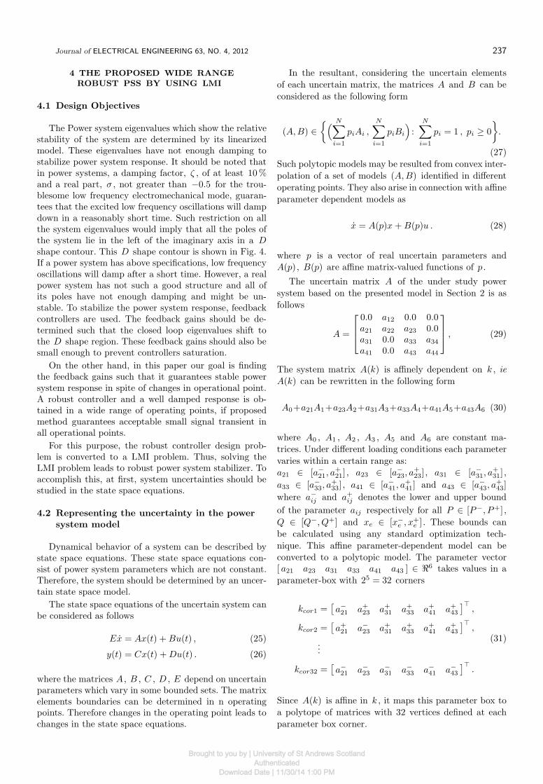
Fig. 5. The response of ∆ω(t) with respect to time in the firstoperating point without using stabilizer

Fig. 6. The response of ∆ω(t) with respect to time in the secondoperating point without using stabilizer

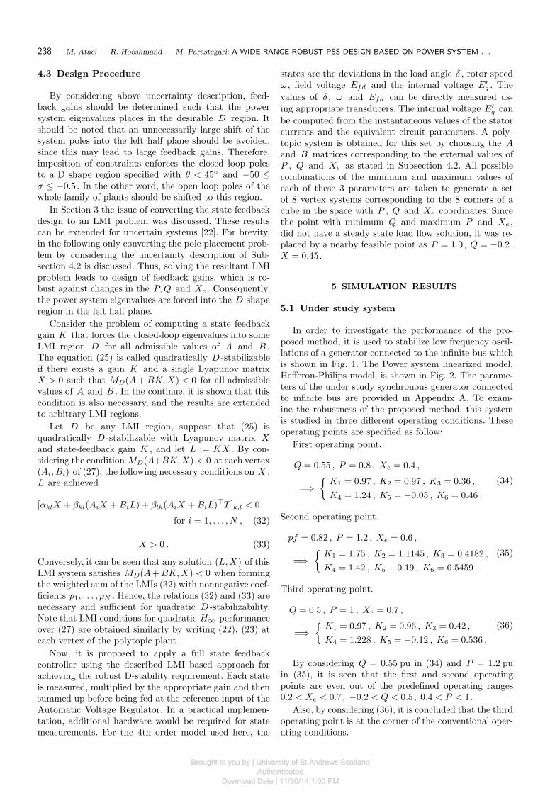
Fig. 7. Closed loop poles with the proposed state feedback con-troller for D shape region pole placement

Fig. 8. Closed loop poles with the proposed state feedback con-troller for oval region pole placement

The performance of the proposed method in three dif-ferent operating points is compared with conventionalPSS to illustrate the proposed method robustness anddesirable dynamic performance. For this purpose, openloop responses of the power system (∆ω(t)) for these op-erating points are shown in Figs. 5 and 6.

5.2 Designing robust stabilizer with pole place-

ment by Solving LMI Problem

By applying the proposed method in Section 4, thefeedback matrix gain is achieved for the under studypower system

k =[

−0.5899466391 292.6014667524

−9.37859374 −0.0407642254]

. (37)

Figure 7 shows the closed loop poles of the set of plantswith the stipulated variations in P , Q and Xe . As seen,the eigenvalues has been shifted into the desired regionof the complex plane for the entire set of plants. AlsoFig. 8 shows closed loop eigenvalues if feedback gainsdetermination problem is solved for oval shaped LMI.

5.3 Designing Conventional PSS

Power system stabilizers can extend power transferstability limits which are characterized by lightly damped

or spontaneously growing oscillations in the 0.2 to 2.5 Hzfrequency range. This is accomplished via excitation con-trol, providing damping to the systems oscillation modes.Consequently, the important issue is the stabilizers abil-ity to enhance damping under the least stable conditions,ie the performance conditions.

Conventional PSS is a controller which stabilize apower system and has a lead-lag transfer function anddamp response of the low frequency oscillations (∆ω ). Ahigh pass filter is used before lead-lag controller to pre-vention harmful effects of the dc signal or very low fre-quency changes. Finally PSS transfer function obtained

like HPSS(s) = KCs1+Tws

T1+sT2+s

form. In this stabilizer T1

and KC are the controller parameters. In this study,we design the conventional PSS for the second operat-ing point.

5.4 Comparison between proposed stabilizer and

conventional PSS

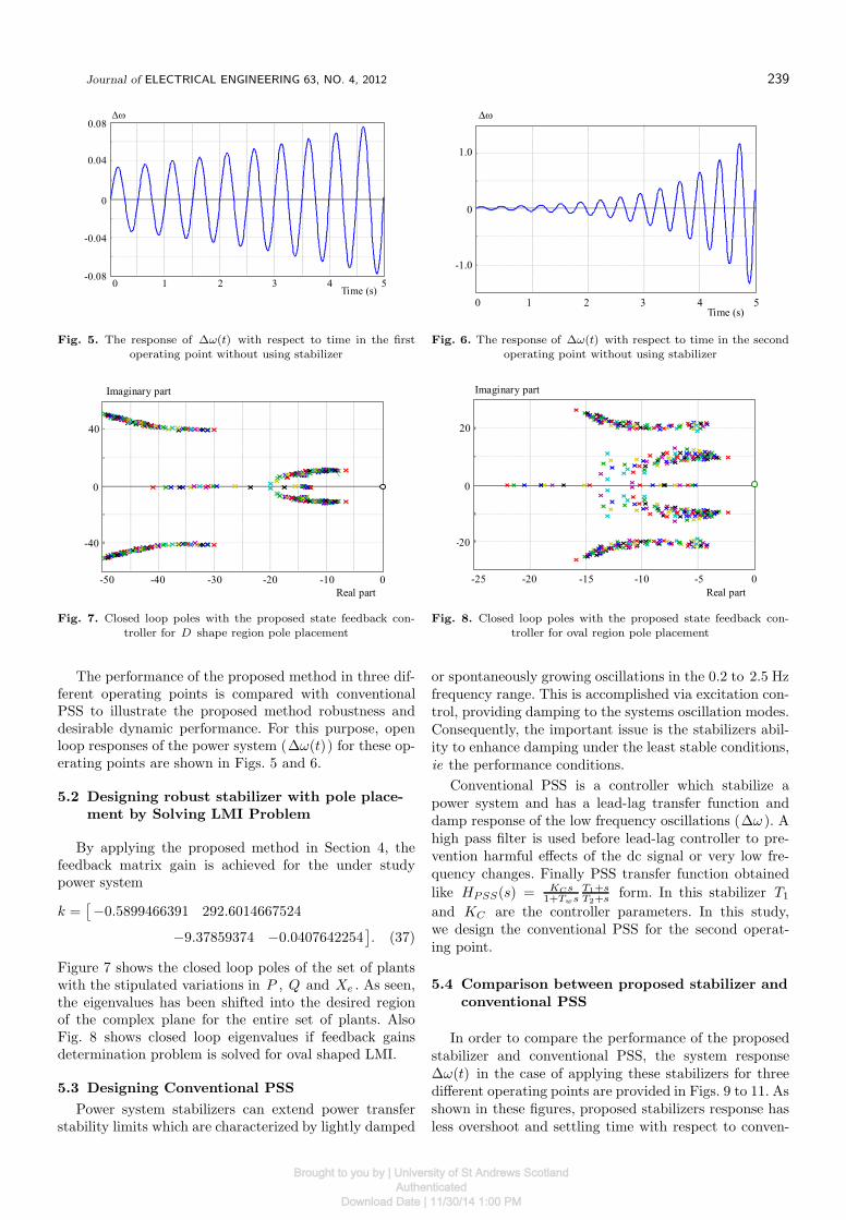
In order to compare the performance of the proposedstabilizer and conventional PSS, the system response∆ω(t) in the case of applying these stabilizers for threedifferent operating points are provided in Figs. 9 to 11. Asshown in these figures, proposed stabilizers response hasless overshoot and settling time with respect to conven-




Fig. 9. The response of ∆ω(t) with respect to time in the firstoperating point by using proposed robust stabilizer compared with

conventional PSS

Fig. 10. The response of ∆ω(t) with respect to time in the secondoperating point by using proposed robust stabilizer and conven-

tional PSS

Fig. 11. The response of ∆ω(t) with respect to time in the thirdoperating point by using proposed robust stabilizer and conven-

tional PSS

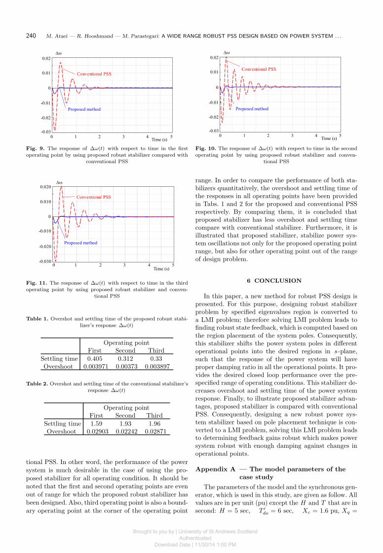
Table 1. Overshot and settling time of the proposed robust stabi-lizer’s response ∆ω(t)

Operating pointFirst Second Third

Settling time 0.405 0.312 0.33Overshoot 0.003971 0.00373 0.003897

Table 2. Overshot and settling time of the conventional stabilizer’sresponse ∆ω(t)

Operating pointFirst Second Third

Settling time 1.59 1.93 1.96Overshoot 0.02903 0.02242 0.02871

tional PSS. In other word, the performance of the powersystem is much desirable in the case of using the pro-posed stabilizer for all operating condition. It should benoted that the first and second operating points are evenout of range for which the proposed robust stabilizer hasbeen designed. Also, third operating point is also a bound-ary operating point at the corner of the operating point

range. In order to compare the performance of both sta-bilizers quantitatively, the overshoot and settling time ofthe responses in all operating points have been providedin Tabs. 1 and 2 for the proposed and conventional PSSrespectively. By comparing them, it is concluded thatproposed stabilizer has less overshoot and settling timecompare with conventional stabilizer. Furthermore, it isillustrated that proposed stabilizer, stabilize power sys-tem oscillations not only for the proposed operating pointrange, but also for other operating point out of the rangeof design problem.

6 CONCLUSION

In this paper, a new method for robust PSS design ispresented. For this purpose, designing robust stabilizerproblem by specified eigenvalues region is converted toa LMI problem; therefore solving LMI problem leads tofinding robust state feedback, which is computed based onthe region placement of the system poles. Consequently,this stabilizer shifts the power system poles in differentoperational points into the desired regions in s-plane,such that the response of the power system will haveproper damping ratio in all the operational points. It pro-vides the desired closed loop performance over the pre-specified range of operating conditions. This stabilizer de-creases overshoot and settling time of the power systemresponse. Finally, to illustrate proposed stabilizer advan-tages, proposed stabilizer is compared with conventionalPSS. Consequently, designing a new robust power sys-tem stabilizer based on pole placement technique is con-verted to a LMI problem, solving this LMI problem leadsto determining feedback gains robust which makes powersystem robust with enough damping against changes inoperational points.

Appendix A — The model parameters of the

case study

The parameters of the model and the synchronous gen-erator, which is used in this study, are given as follow. Allvalues are in per unit (pu) except the H and T that are insecond: H = 5 sec, T ′

do = 6 sec, Xc = 1.6 pu, Xq =




1.55 pu, X ′d = 0.32 pu Also, the system excita-

tion parameters are KA = 400, KF = 0.025, TA =0.05 sec, TF = 1 sec. Moreover, the parameters, whichare used in the controller design, are

P1-self-tuning = −1.07 , P2-self-tuning = 0.6376 ,

ωconventional-PSS = 7.6 , ζconventional-PSS = 0.2 ,

T2-conventional-PSS = 0.2 , Kconventional-PSS = 5.622 .

References

[1] ANDERSON, P. M.—FOUAD, A. A. : Power System Controland Stability, IEEE Press, 2002.

[2] YU, Y. N. : Electric Power System Dynamic Stability, Academicpress, 1983.

[3] ATAEI, M.—HOOSHMAND, R.—PARASTEGARI, M. : Self-Tuning Power System Stabilizer Design Based on Pole Assign-ment and Pole-Shifting Techniques, Journal of Applied Sciences8 No. 8 (2008), 1406–1415.

[4] WERNER, H.—KORBA, P.—YANG, T. C. : Robust Tuning ofPower System Stabilizers Using LMI-Techniques, IEEE Trans.on Control Systems Technology 11 No. 1 (Jan 2003), 147–152.

[5] SOLIMAN, M.—EMARA, H.—ELSHAFEI, A.—BAHGAT,A.—MALIK, O. P. : Robust Output Feedback Power SystemStabilizer Design: an LMI Approach, IEEE Power and EnergySociety General Meeting – Conversion and Delivery of ElectricalEnergy in the 21st Century, July 2008, pp. 1-8.

[6] CHILALI, M.—GAHINET, P. : H∞ Design with Pole Place-

ment Constraints: An LMI approach, IEEE Trans. on AutomaticControl 41 No. 3 (Mar 1996), 358–367.

[7] RAO, P. S.—SEN, I. : Robust Pole Placement Stabilizer DesignUsing Linear Matrix Inequalities, IEEE Trans. Power Systems15 No. 1 (Feb 2000), 313–319.

[8] GUPTA, R.—BHATIA, D. : Comparison of Robust Fuzzy Logicand Fast Output Sampling Feedback Based Power System Sta-bilizer for SMIB, IEEE International Conf. on Industrial Tech-nology, Dec 2006, pp. 1031-1036.

[9] CHOW, J. T.—HARRIS, P.—OTHMAN, H. A.—SNNCHEA-GUSCA, J. J.—TERWILLIGER, C. E. : Robust Control Designof Power System Stabilizers Using Multivariable Frequency Do-

main Techniques, in Proc. 29th IEEE Conf. on Decision andControl, Hawai, Dec 1990, pp. 2067-2073.

[10] SCAVONI, F. E.—de SILVA, A. S.—NETO, A. T.—CAMPA-GNOLO, J. M. : Design of Robust Power System Controllersusing Linear Matrix Inequalities, Proc. 2001 IEEE Porto PowerTech Conf., vol. 2, Sep 2001, pp. 1–6.

[11] JIANYING, H. G.—RONG, X.—WEIGUO, L.—SHUANQIN,X. : H Infinity Controller Design of the Synchronous Generator,International Conference on Intelligent Computation Technol-ogy and Automation (ICICTA), vol. 1, Oct 2008, pp. 370-374.

[12] DEHGHANI, M.—NIKRAVESH, S. K. Y. : Robust Tuning ofPSS Parameters Using the Linear Matrix Inequalities Approach,IEEE Power Tech 2007 Lausanne, July 2007, pp. 322-326.

[13] JOO, K. S.—MOON, K. S.—HYUN, Y.—KOOK-HUN, K. :Low-Order Robust Power System Stabilizer for Single-Machine

Systems: an LMI Approach, 32nd Annual IEEE Conf. on Indus-trial Electronics, IECON 2006, Nov 2006, pp. 742-747.

[14] GUPTA, R.—BANDYOPADHYAY, B.—KULKARNI, A. M. :Design of Power System Stabilizer for Single-Machine Sys-tem using Robust Periodic Output Feedback Controller, Proc.2003 IEE Generator Transmission Distribution Conf., vol. 150,Mar 2003, pp. 211–216.

[15] JIANYING, G.—RONG, X.—WEIGUO, L.—SHUANQIN, X. :

H∞ Controller Design of the Synchronous Generator, Inter-

national Conf on Intelligent Computation Technology and Au-

tomation (ICICTA), vol. 1, Oct 2008, pp. 370-374.

[16] SHIAU, J. K.—CHOW, J. H.—BOUKARIM, G. : Power Swing

Damping Controller Design using Linear Matrix Inequality Al-

gorithm, Proc. IEEE Conf Control Application, vol. 2, Sep 1996,

pp. 727–732.

[17] El-RAZAZ, Z. S.—MANDOR, M. E. D.—ALI, E. S. : Damping

Controller Design for Power Systems Using LMI and GA Tech-niques, Proceedings of the 41st International Universities Power

Engineering Conf., vol. 2, Sep 2006, pp. 500-506.

[18] JUHUA,—KROGH, B. H.—ILIC, M. D. : Saturation-Induced

Frequency Instability in Electric Power Systems, IEEE Power

and Energy Society General Meeting – Conversion and Delivery

of Electrical Energy in the 21st Century, July 2008, pp. 1-7.

[19] BEVRANI, H.—HIYAMA, T. : Stability and Voltage Regula-

tion Enhancement using an Optimal Gain Vector, Proc. IEE

Power Engineering Society Conf., June 2006, pp. 1–8.

[20] BOYD, S.—FERON, E.—BALAKRISHNAN, V.—GHAOUI,

E. L. : Linear Matrix Inequalities in System and Control The-

ory, Studies in Applied Mathematics, SIAM, Philadelphia PA,

1994.

[21] GAHINET, P.—NEMIKOVSKI, A.—LAUR, A. J.—CHILALI,

M. : LMI Control Toolbox for use with Matlab, The Mathworks

Inc., Natick, MA, 1995.

[22] CHILALI, M.—GAHINET, P. : H∞ Design with Pole Place-

ment Constraints: An LMI Approach, IEEE Trans. Automatic

Control 41 No. 3 (Mar 1996), 358–367.

Received 31 May 2010

Mohammad Ataei (1971) received the BS degree from

the Isfahan University of Technology, Iran, in 1994, the MS de-gree from the Iran University of Science & Technology, Iran, in1997, and PhD degree from K. N. Toosi University of Technol-

ogy, Iran, in 2004 all in Electrical Engineering. He has done hisPhD project jointly with the University of Bremen in Germanyfrom 2001 till 2003. Since 2004, he is with the Department of

Electrical Engineering at the University of Isfahan, Iran. Hehas worked on time series analysis of chaotic systems, robustcontrol, control theory and applications. His main areas of re-

search interest are also chaos control and synchronization, andnonlinear control.

Rahmat-Allah Hooshmand (1967) received the BSEEdegree from the University of Mashhad in 1989, the MSEE

from the University of Tehran/Iran and PhD degree from Tar-biat Modarres University/Iran in 1990 and 1995, respectivelyall in Electrical Engineering. Since 1995, he is with the De-

partment of Electrical Engineering at the University of Isfa-han/Iran, as an associate professor. His main areas of researchinterest are modeling of Power Systems and Distribution Net-

works.

Moein Parastegari (1983) was born in Isfahan in the Is-lamic Republic of Iran, on March 30, 1983. He received BSDegree in Electrical Engineering from Shahrekord University,

Iran, in 2005. He received MS Degree in Electrical Engineer-ing from University of Isfahan, Iran, in 2008. Currently, he isworking towards the PhD Degree in power system from Isfa-

han University, Isfahan, Iran. His research interests are in thearea of power systems control and operation.



a wide range robust pss design based on power system pole-placement using linear matrix inequality

Documents