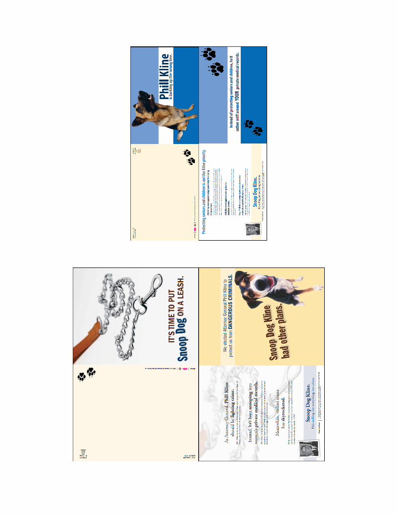
A.1 Pictures of Mailings

Each picture is the front and back of a postcard mailed by the vendor, displayed in their

order of receipt

A.2 Local Linear Regression

Bandwidth Selection

To select the bandwidth for the local linear regressions, we implement a leave-one-out

cross-validation procedure similar to that proposed by Ludwig and Miller (2005). The procedure

starts by fixing a bandwidth s. Select a census block c’ with values of forcingc’ > 0, and estimate a

local linear regression with a bandwidth parameter of s using all of the census blocks with forcingc

> 0, except census block c’. Use the estimated function to construct a fitted vote share, 'ˆcY , for the

excluded census block. Do this for each of the N+ observations with forcingc > 0, and find the

average squared difference between the actual and fitted values. Repeat this procedure for census

blocks with values of forcing below the income threshold. Our measure of the goodness-of-fit for

a given bandwidth s is:

2

0

2

0

)ˆ(2

1)ˆ(

2

1)( c

forcing

cc

forcing

c YYN

YYN

sCVcc

−+−= ∑∑<<+<<−− δδ

δ .

The bandwidth is selected by finding the value of s that minimizes CV(s)δ. The smaller

the value of δ, the smaller the range around the discontinuous threshold that is considered when

assessing the goodness-of-fit. Below is a graph of the value of CV(s) for δ = {1, 2, 3} for the

DDD estimator using a rectangle kernel. We observe that CV(s) is relatively flat for values of s

between 1 and 4. When δ = {2, 3}, the value of CV(s) is minimized at s = 1.57, while for δ = 1

CV(s) is minimized at s = 3.46.

0.0055

0.006

0.0065

0.007

0.0075

0.5

0.7

5 1

1.2

5

1.5

1.7

5 2

2.2

5

2.5

2.7

5 3

3.2

5

3.5

3.7

5 4

4.2

5

4.5

4.7

5 5

Bandwidth (s)

δ= 2 δ = 1 δ= 3

Figure A1: Values of Cross-Validation Function by Bandwidth and Range

Graphical Analysis

0.1

.2.3

.4%

in M

aile

d H

H

-5 0 5forcing

Figure A2: Local Linear Regression of Mail Concentration in 2006 by Majority Census

Block Group Income (bandwidth = 1.57, rectangle kernel)

.3.4

.5.6

.7%

Dem

. A

G '0

6

-5 0 5forcing

Figure A3: Local Linear Regression of Democratic Attorney General Vote Share in 2006

by Majority Census Block Group Income (bandwidth = 1.57, rectangle kernel)

-.2

-.1

0.1

.2%

Dem

. A

G '0

6 -

% D

em

. G

ov. '0

6

-5 0 5forcing

Figure A4: Local Linear Regression of Difference in Democratic AG and Governor Vote

Shares in 2006 by Majority Census Block Group Income (bandwidth = 1.57, rectangle

kernel)

-.2

-.1

0.1

.2A

G-G

ov D

iff. '0

6 -

AG

-Go

v D

iff. 0

2

-5 0 5forcing

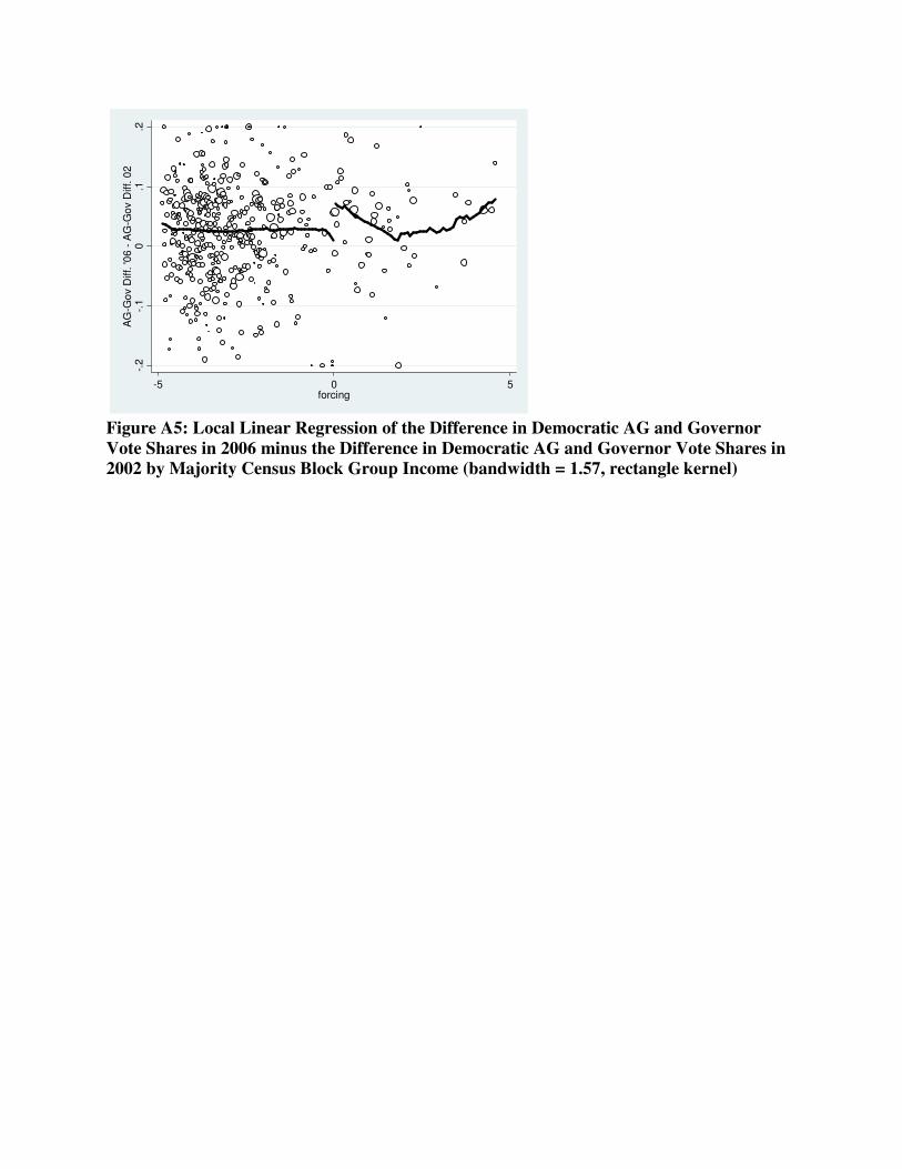
Figure A5: Local Linear Regression of the Difference in Democratic AG and Governor

Vote Shares in 2006 minus the Difference in Democratic AG and Governor Vote Shares in

2002 by Majority Census Block Group Income (bandwidth = 1.57, rectangle kernel)

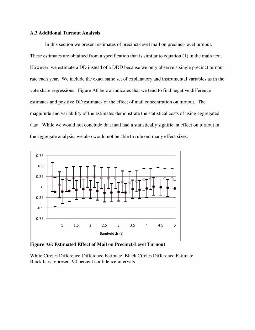
A.3 Additional Turnout Analysis

In this section we present estimates of precinct-level mail on precinct-level turnout.

These estimates are obtained from a specification that is similar to equation (1) in the main text.

However, we estimate a DD instead of a DDD because we only observe a single precinct turnout

rate each year. We include the exact same set of explanatory and instrumental variables as in the

vote share regressions. Figure A6 below indicates that we tend to find negative difference

estimates and positive DD estimates of the effect of mail concentration on turnout. The

magnitude and variability of the estimates demonstrate the statistical costs of using aggregated

data. While we would not conclude that mail had a statistically significant effect on turnout in

the aggregate analysis, we also would not be able to rule out many effect sizes.

-0.75

-0.5

-0.25

0

0.25

0.5

0.75

1 1.5 2 2.5 3 3.5 4 4.5 5

Bandwidth (s)

Figure A6: Estimated Effect of Mail on Precinct-Level Turnout

White Circles Difference-Difference Estimate, Black Circles Difference Estimate

Black bars represent 90 percent confidence intervals