AA203Optimal and Learning-based Control

Course overview, nonlinear optimization

Course mechanics

Teaching team:• Instructor: Marco Pavone• CAs: James Harrison and Jonathan Lacotte• Collaborators: Riccardo Bonalli (Stanford) and Roberto Calandra (FAIR)

Logistics:• Class info, lectures, and homework assignments on class web page:

http://asl.stanford.edu/aa203/• Forum: https://piazza.com/

4/1/19 AA 203 | Lecture 1 2

Course requirements

• Weekly homework, due Wednesday• Midterm exam (05/02)• Final project (more details later)• Grading:• homework 30% • midterm 30%• final project 35%• grading quality 5%

4/1/19 AA 203 | Lecture 1 3

Prerequisites

• Strong familiarity with calculus (e.g., CME100)• Strong familiarity with linear algebra (e.g., EE263 or CME200)

4/1/19 AA 203 | Lecture 1 4

Outline

1. Problem formulation and course goals

2. Non-linear optimization

3. Computational methods

4/1/19 AA 203 | Lecture 1 5

Outline

1. Problem formulation and course goals

2. Non-linear optimization

3. Computational methods

4/1/19 AA 203 | Lecture 1 6

Problem formulation

• Mathematical description of the system to be controlled• Statement of the constraints• Specification of a performance criterion

4/1/19 AA 203 | Lecture 1 7

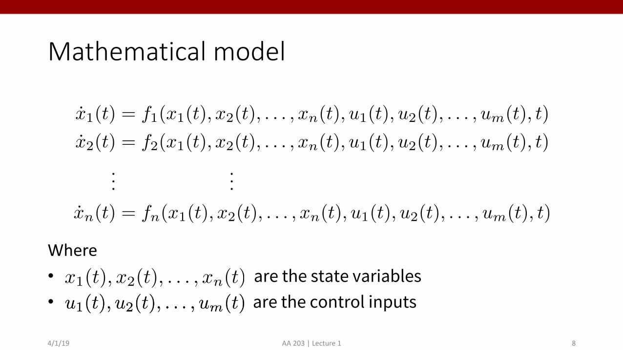
Mathematical model

Where• are the state variables• are the control inputs

4/1/19 AA 203 | Lecture 1 8

x1(t) = f1(x1(t), x2(t), . . . , xn(t), u1(t), u2(t), . . . , um(t), t)

x2(t) = f2(x1(t), x2(t), . . . , xn(t), u1(t), u2(t), . . . , um(t), t)

......

xn(t) = fn(x1(t), x2(t), . . . , xn(t), u1(t), u2(t), . . . , um(t), t)

x1(t), x2(t), . . . , xn(t)

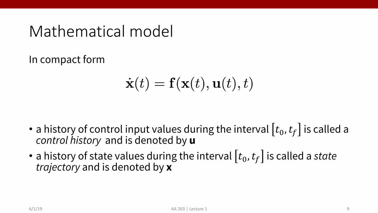
Mathematical model

• a history of control input values during the interval !", !$ is called a control history and is denoted by u• a history of state values during the interval !", !$ is called a state

trajectory and is denoted by x

4/1/19 AA 203 | Lecture 1 9

In compact form

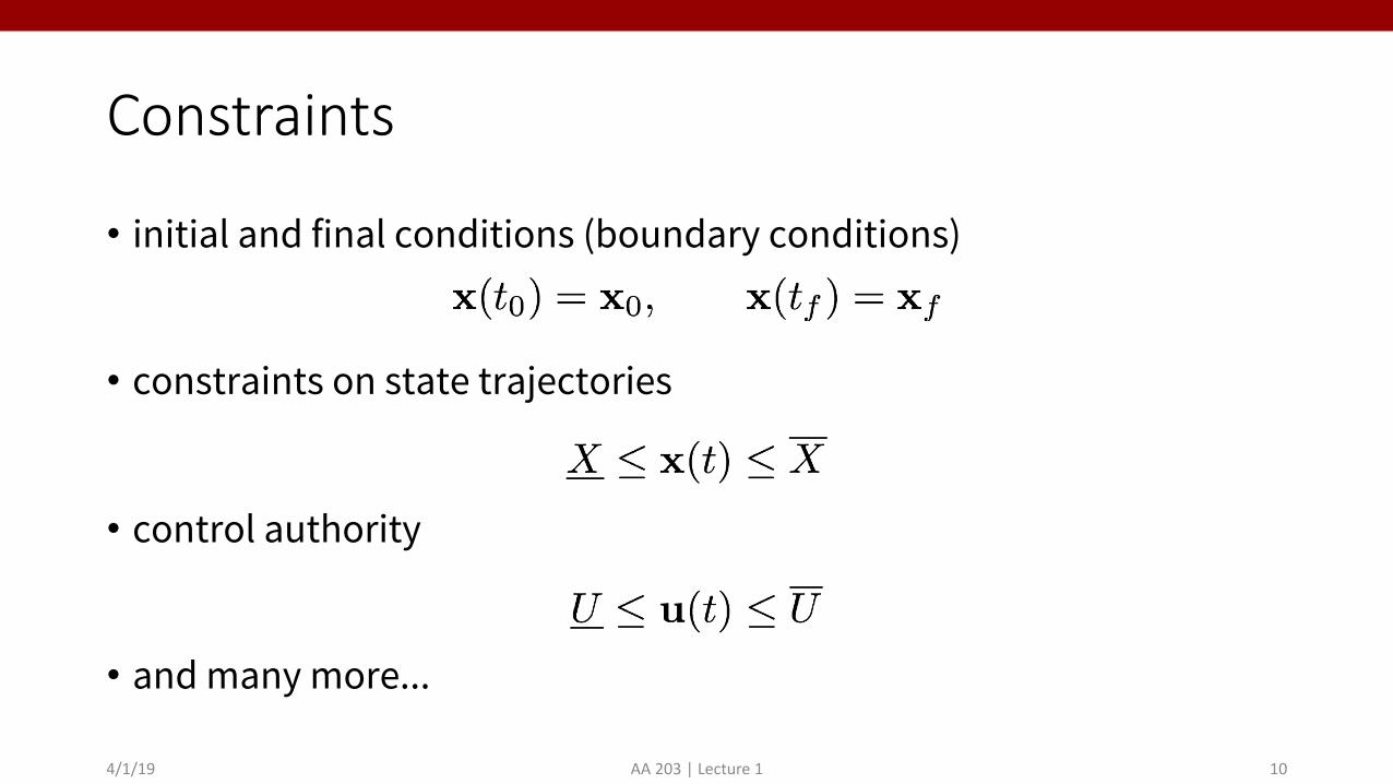
Constraints

• initial and final conditions (boundary conditions)

• constraints on state trajectories

• control authority

• and many more...

4/1/19 AA 203 | Lecture 1 10

Constraints

• A control history which satisfies the control constraints during the entire time interval !", !$ is called an admissible control • A state trajectory which satisfies the state variable constraints

during the entire time interval !", !$ is called an admissible trajectory

4/1/19 AA 203 | Lecture 1 11

Performance measure

• ℎ and " are scalar functions• #$ may be specified or free

4/1/19 AA 203 | Lecture 1 12

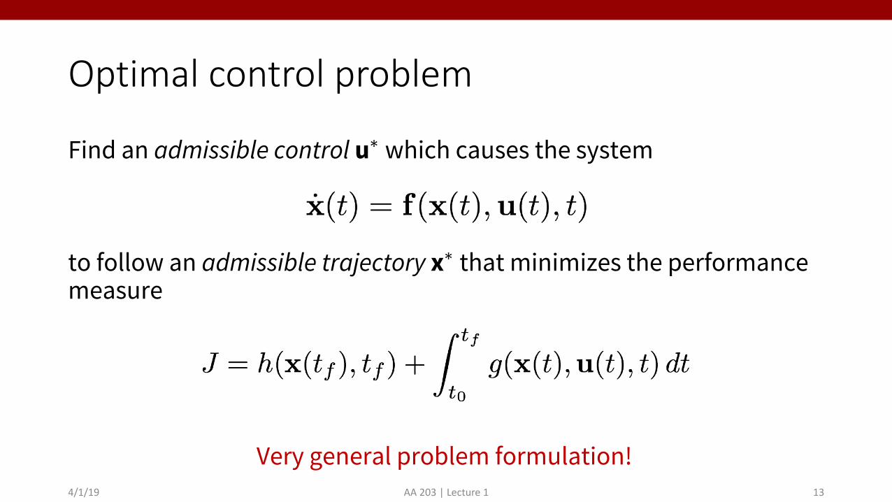
Optimal control problem

Find an admissible control u∗ which causes the system

to follow an admissible trajectory x∗ that minimizes the performance measure

4/1/19 AA 203 | Lecture 1 13

Very general problem formulation!

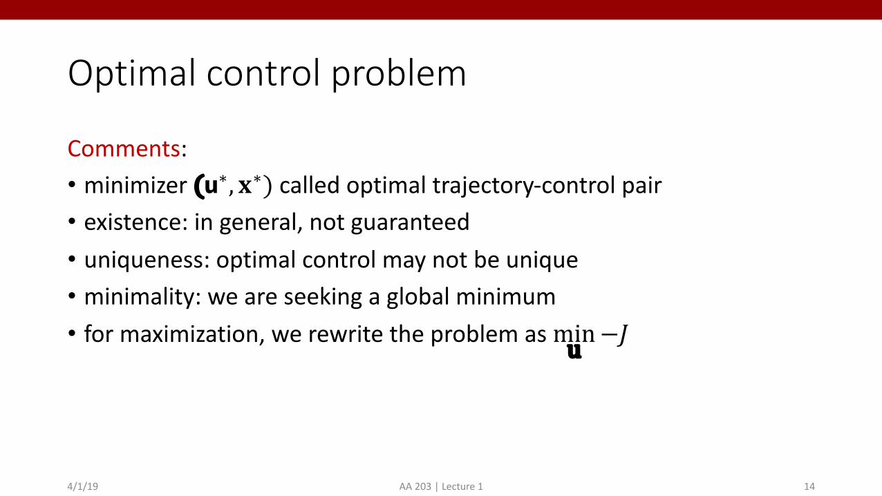
Optimal control problem

Comments:• minimizer (u∗, $∗) called optimal trajectory-control pair• existence: in general, not guaranteed• uniqueness: optimal control may not be unique• minimality: we are seeking a global minimum• for maximization, we rewrite the problem as minu −+

4/1/19 AA 203 | Lecture 1 14

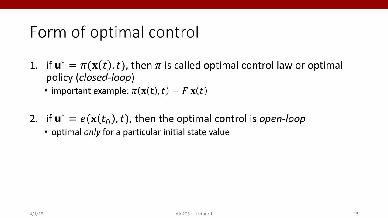
Form of optimal control

1. if u∗ = #(% & , &), then # is called optimal control law or optimal policy (closed-loop)• important example: # % t , & = * % &

2. if u∗ = +(% &, , &), then the optimal control is open-loop• optimal only for a particular initial state value

4/1/19 AA 203 | Lecture 1 15

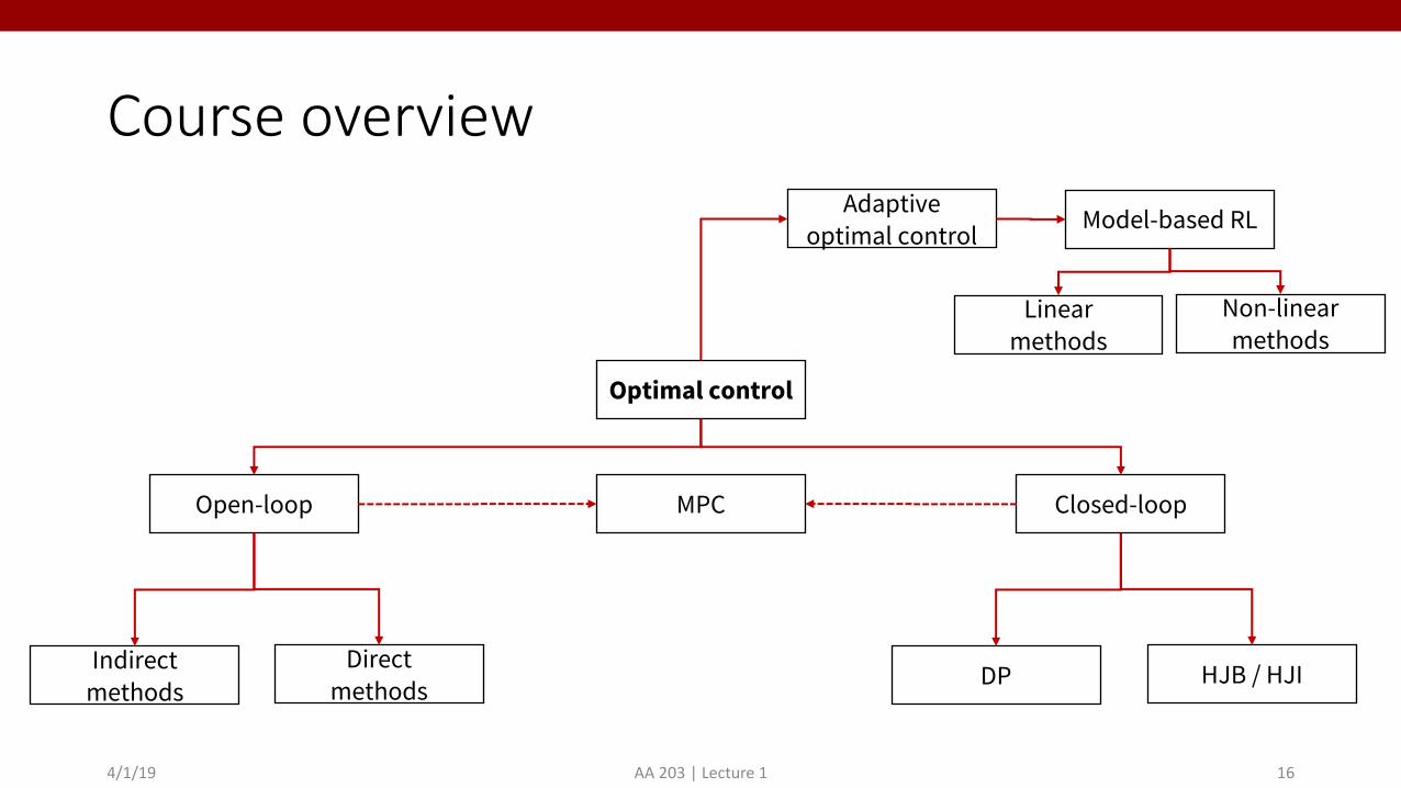
Course overview

4/1/19 AA 203 | Lecture 1 16

Optimal control

Open-loop

Indirect methods

Direct methods

Closed-loop

DP HJB / HJI

MPC

Adaptiveoptimal control Model-based RL

Linear methods

Non-linear methods

Course goals

To learn the theoretical and implementation aspects of main techniques in optimal control and model-based reinforcement learning

AA 203 | Lecture 1 174/1/19

Outline

1. Problem formulation and course goals

2. Non-linear optimization

3. Computational methods

4/1/19 AA 203 | Lecture 1 18

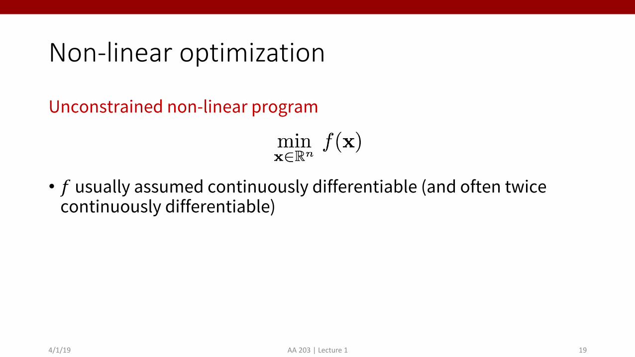
Non-linear optimization

Unconstrained non-linear program

• ! usually assumed continuously differentiable (and often twice continuously differentiable)

4/1/19 AA 203 | Lecture 1 19

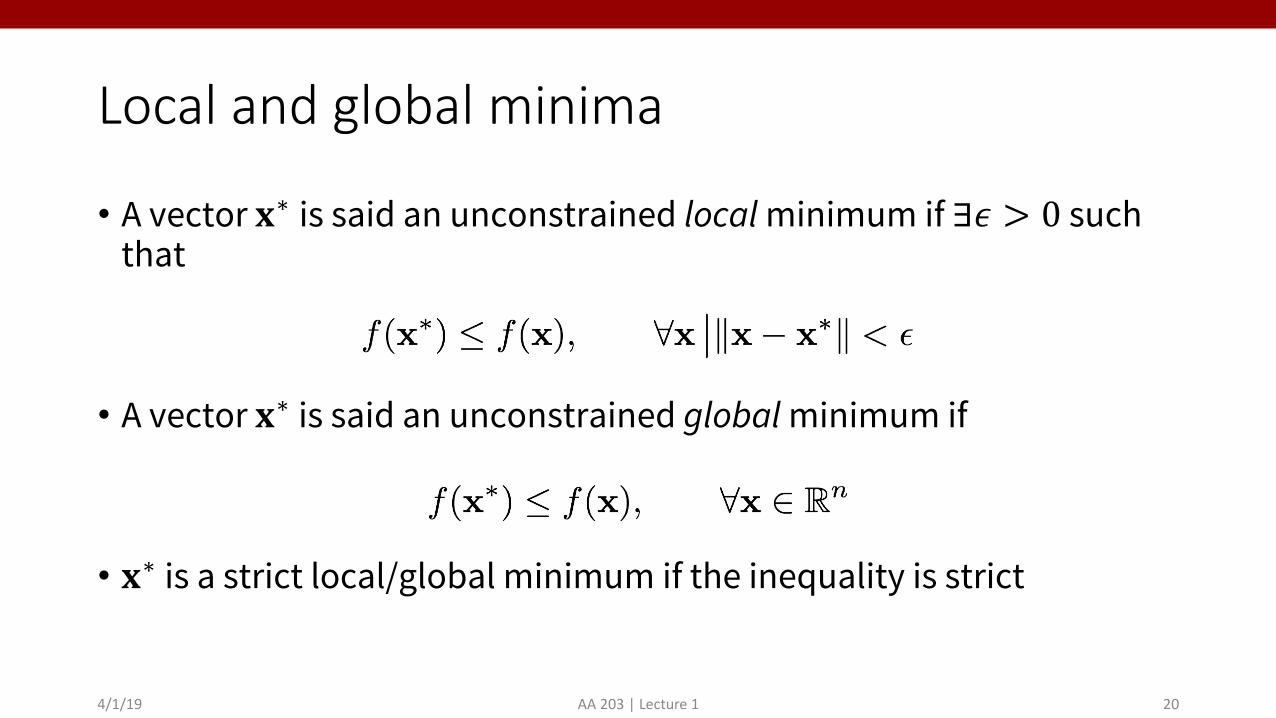
Local and global minima

• A vector !∗ is said an unconstrained localminimum if ∃$ > 0 such that

• A vector !∗ is said an unconstrained globalminimum if

• !∗ is a strict local/global minimum if the inequality is strict

4/1/19 AA 203 | Lecture 1 20

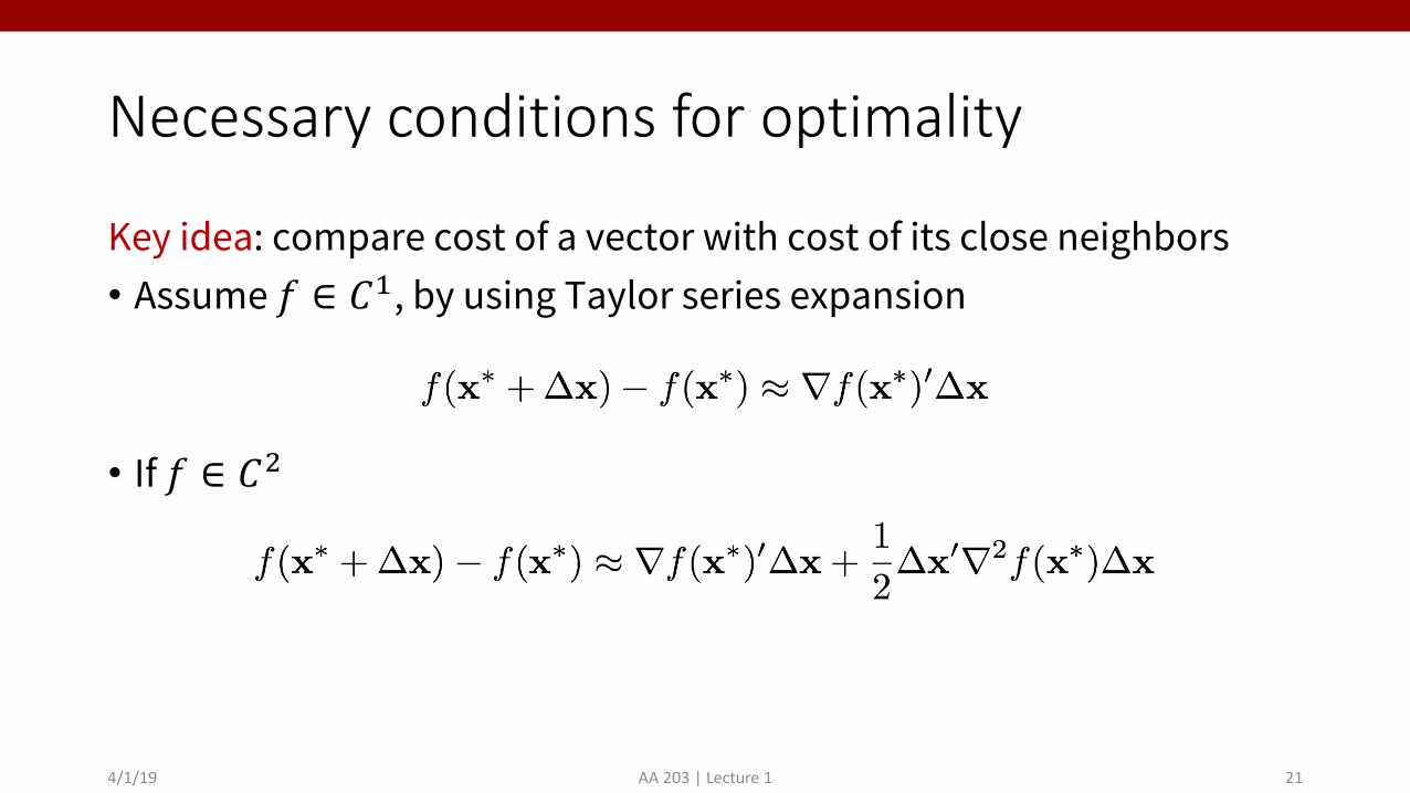
Necessary conditions for optimality

Key idea: compare cost of a vector with cost of its close neighbors• Assume ! ∈ #$, by using Taylor series expansion

• If ! ∈ #%

4/1/19 AA 203 | Lecture 1 21

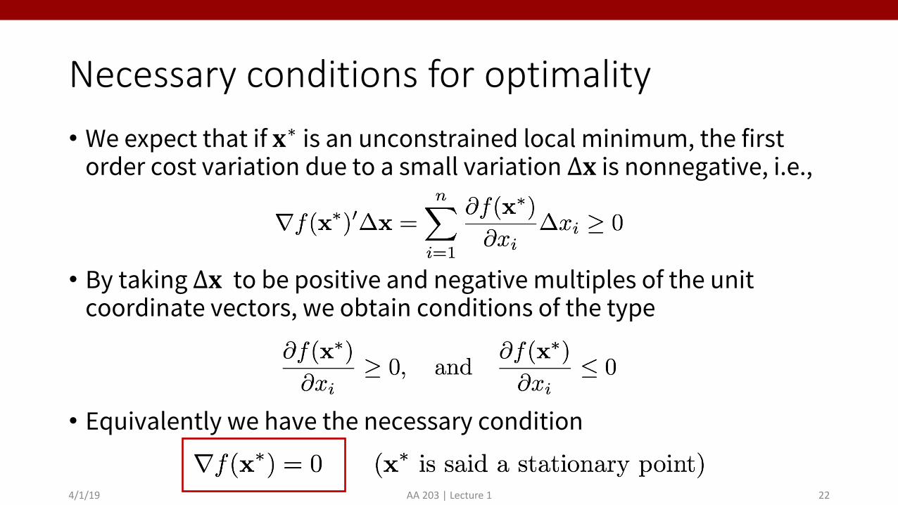
Necessary conditions for optimality• We expect that if !∗ is an unconstrained local minimum, the first

order cost variation due to a small variation Δ! is nonnegative, i.e.,

• By taking Δ! to be positive and negative multiples of the unit coordinate vectors, we obtain conditions of the type

• Equivalently we have the necessary condition

4/1/19 AA 203 | Lecture 1 22

Necessary conditions for optimality

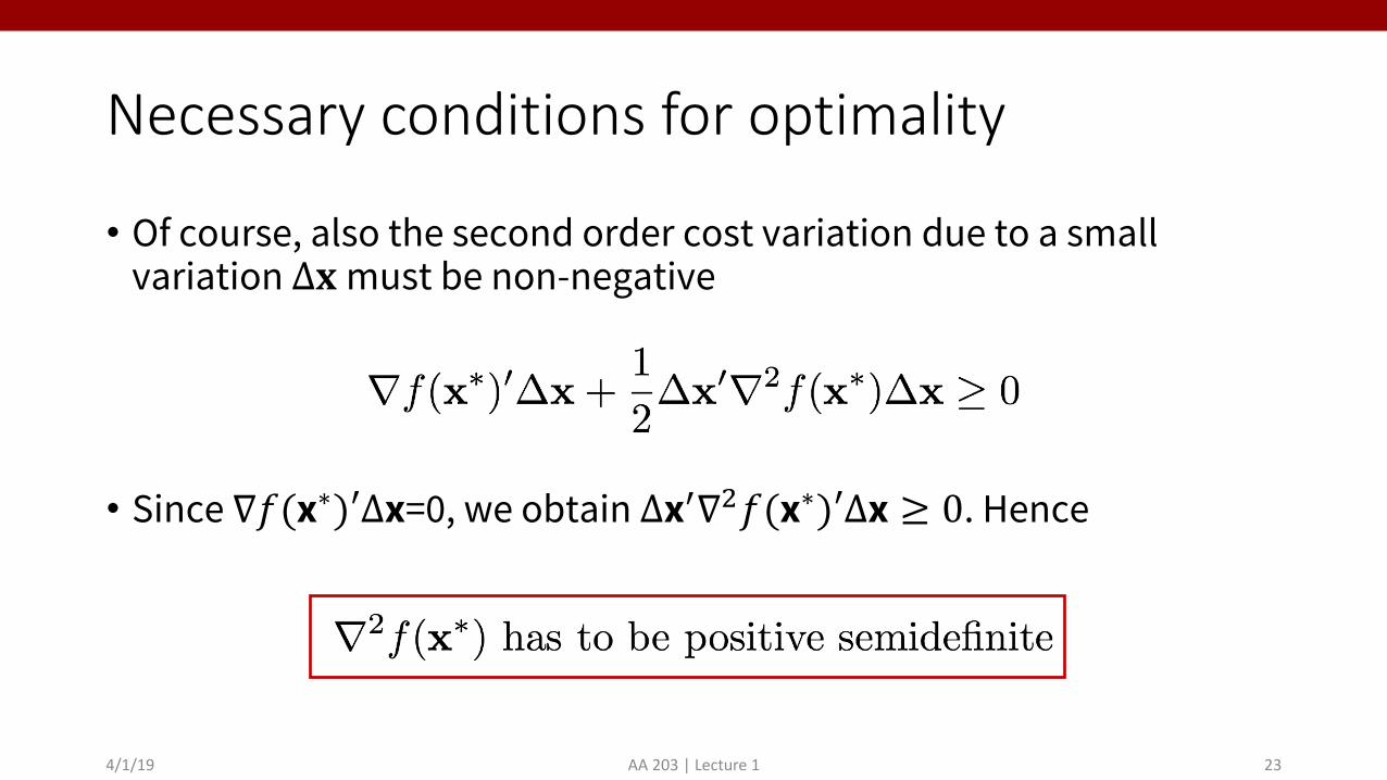
• Of course, also the second order cost variation due to a small variation Δ" must be non-negative

• Since ∇$(x∗)′∆x=0, we obtain ∆x*∇+$(x∗)′∆x ≥ 0. Hence

4/1/19 AA 203 | Lecture 1 23

NOC – formal

Theorem: NOC Let !∗be an unconstrained local minimum of #:ℝ& ↦ℝ and assume that # is () in an open set * containing !∗. Then

If in addition # ∈ (, within *,

4/1/19 AA 203 | Lecture 1 24

(first order NOC)

positive semidefinite (second order NOC)

SOC

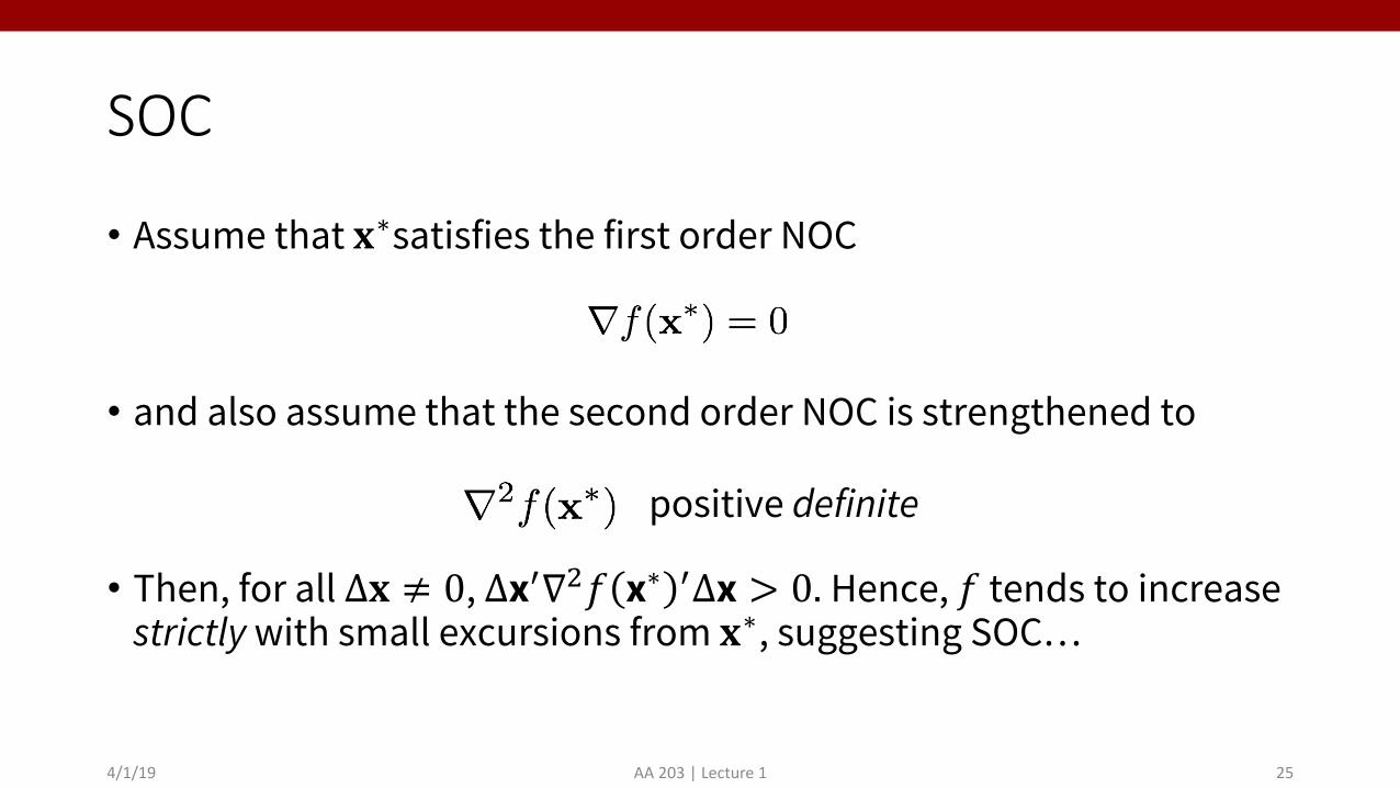
• Assume that !∗satisfies the first order NOC

• and also assume that the second order NOC is strengthened to

• Then, for all Δ! ≠ 0, ∆x'∇)* x∗ '∆x > 0. Hence, * tends to increase strictlywith small excursions from !∗, suggesting SOC…

4/1/19 AA 203 | Lecture 1 25

positive definite

SOC

4/1/19 AA 203 | Lecture 1 26

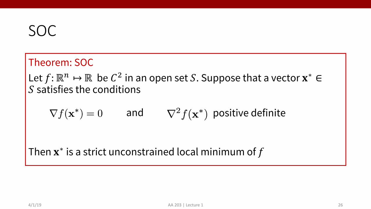
Theorem: SOC Let #:ℝ& ↦ℝ be () in an open set *. Suppose that a vector +∗ ∈* satisfies the conditions

Then +∗ is a strict unconstrained local minimum of #

and positive definite

Special case: convex optimization

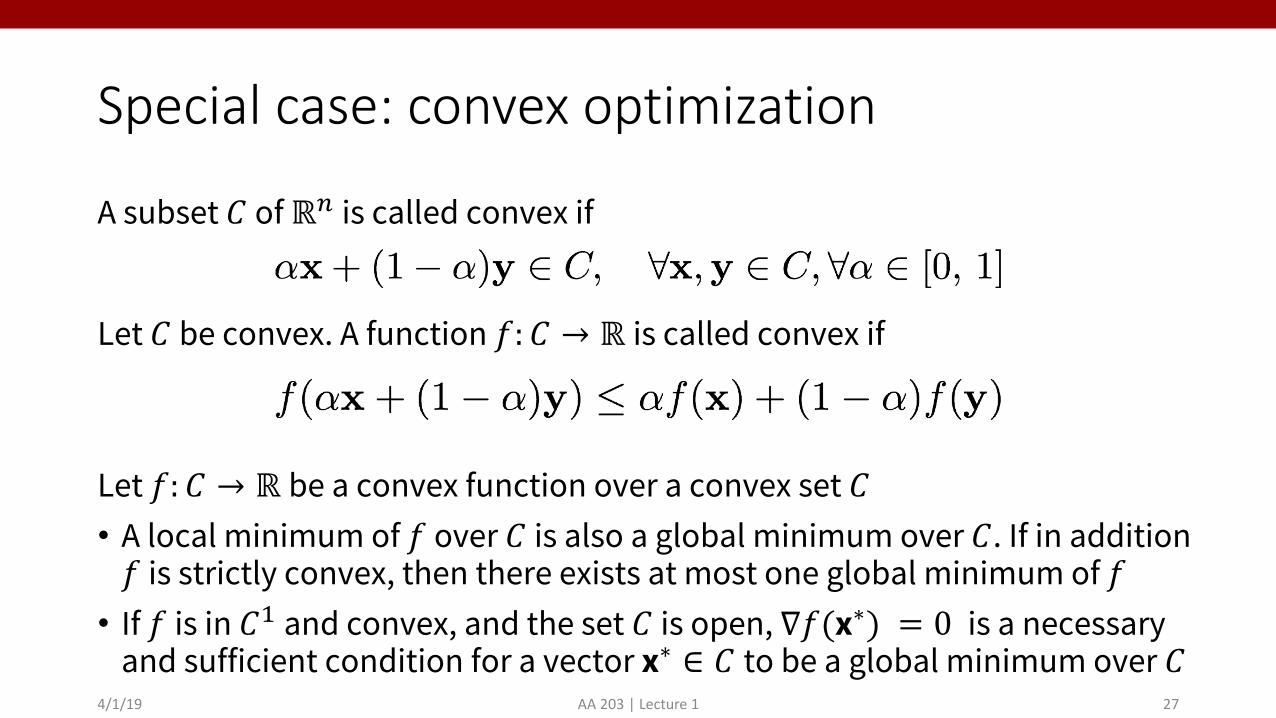
A subset ! of ℝ# is called convex if

Let ! be convex. A function $: ! → ℝ is called convex if

Let $: ! → ℝ be a convex function over a convex set !• A local minimum of $ over ! is also a global minimum over !. If in addition $ is strictly convex, then there exists at most one global minimum of $• If $ is in !' and convex, and the set ! is open, ∇$(x∗) = 0 is a necessary

and sufficient condition for a vector x∗ ∈ ! to be a global minimum over !4/1/19 AA 203 | Lecture 1 27

Discussion

• Optimality conditions are important to filter candidates for global minima • They often provide the basis for the design and analysis of

optimization algorithms• They can be used for sensitivity analysis

4/1/19 AA 203 | Lecture 1 28

Outline

1. Problem formulation and course goals

2. Non-linear optimization

3. Computational methods

4/1/19 AA 203 | Lecture 1 29

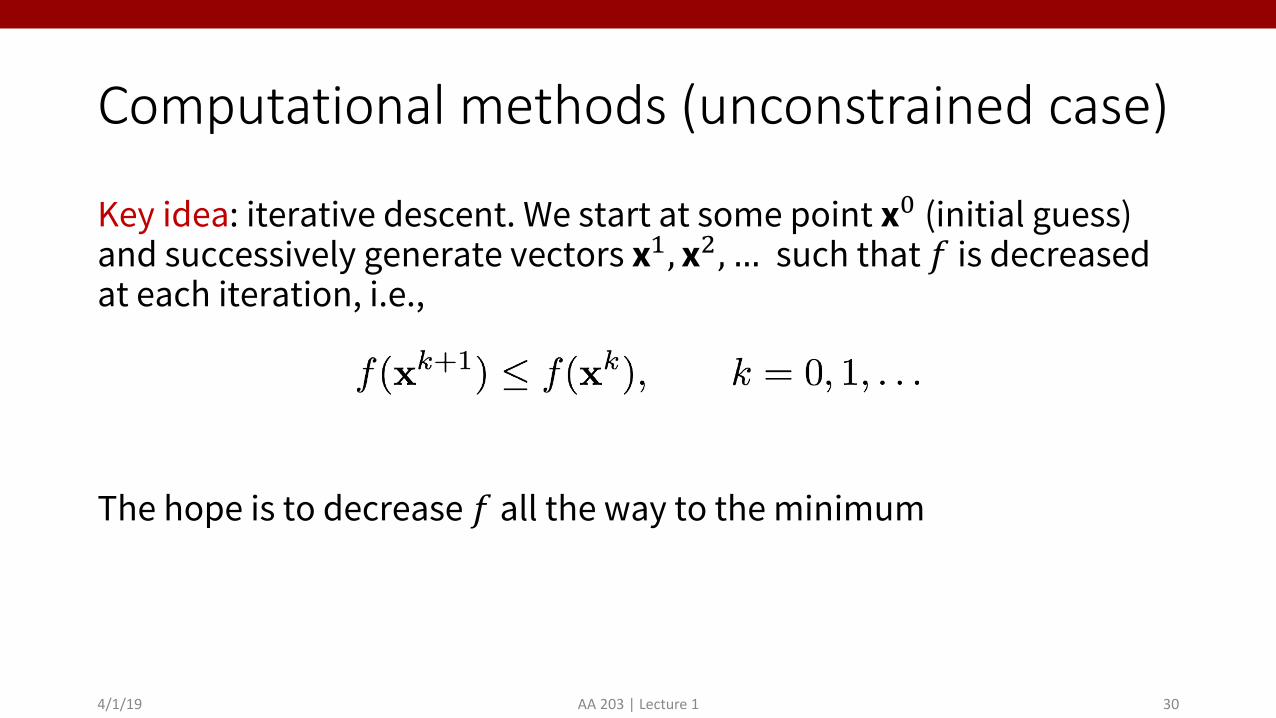
Computational methods (unconstrained case)

Key idea: iterative descent. We start at some point x! (initial guess) and successively generate vectors x", x$, … such that & is decreased at each iteration, i.e.,

The hope is to decrease & all the way to the minimum

4/1/19 AA 203 | Lecture 1 30

Gradient methods

Given x ∈ ℝ# with ∇% & ≠ 0, consider the half line of vectors

From first order Taylor expansion () small)

So for ) small enough %(&+) is smaller than %(&)!

4/1/19 AA 203 | Lecture 1 31

Gradient methods

Carrying this idea one step further, consider the half line of vectors

where ∇" # $% < ' (angle > 90∘)

By Taylor expansion

For small enough ,, "(# + ,%) is smaller than "(#)!

4/1/19 AA 203 | Lecture 1 32

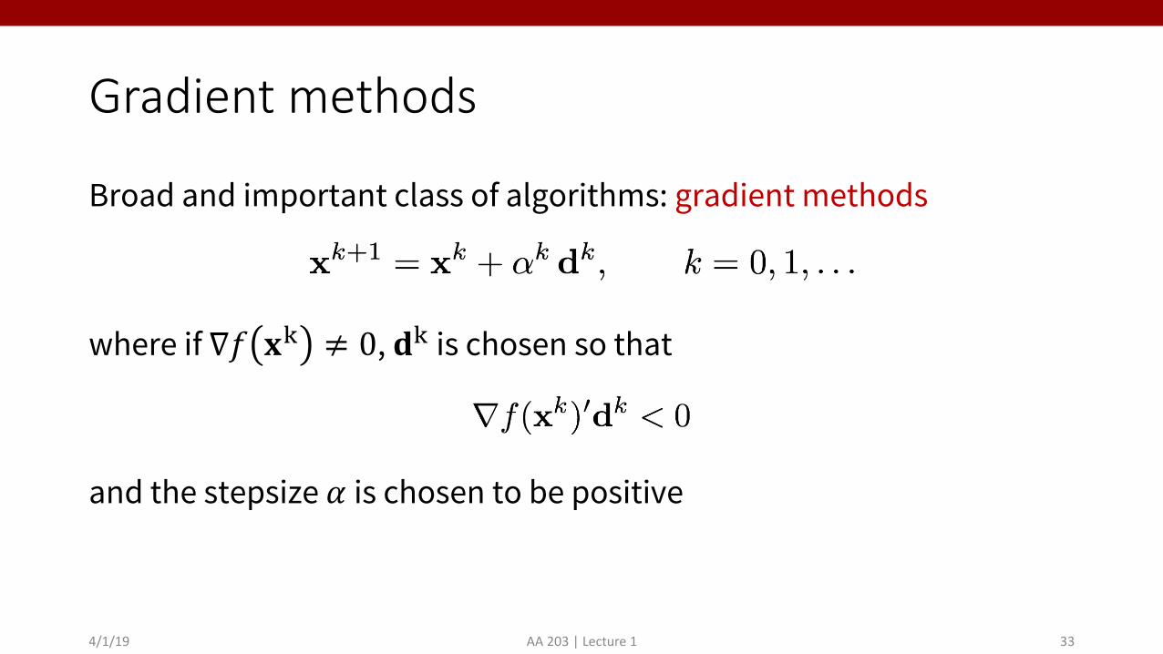
Gradient methods

Broad and important class of algorithms: gradient methods

where if ∇" #$ ≠ 0, '$ is chosen so that

and the stepsize ( is chosen to be positive

4/1/19 AA 203 | Lecture 1 33

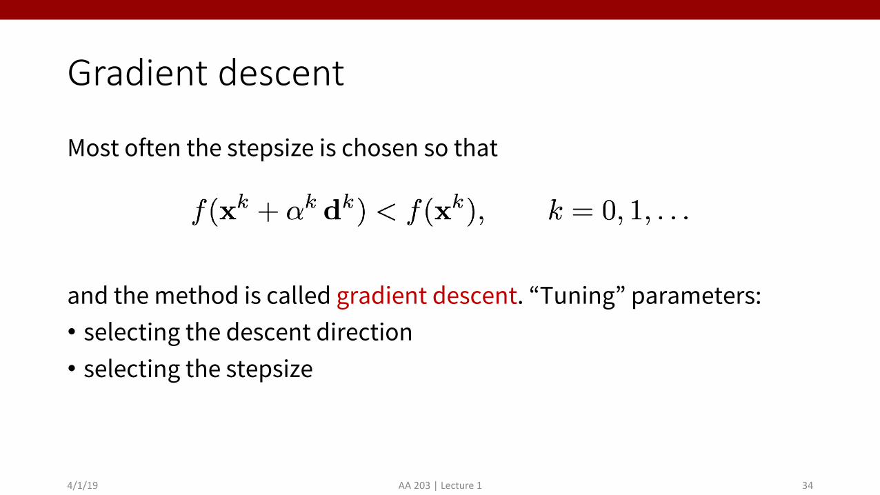
Gradient descent

Most often the stepsize is chosen so that

and the method is called gradient descent. “Tuning” parameters:• selecting the descent direction• selecting the stepsize

4/1/19 AA 203 | Lecture 1 34

Selecting the descent direction

General class

(Obviously, ∇" #$ %&$ < 0)

Popular choices:• Steepest descent:

• Newton's method: provided

4/1/19 AA 203 | Lecture 1 35

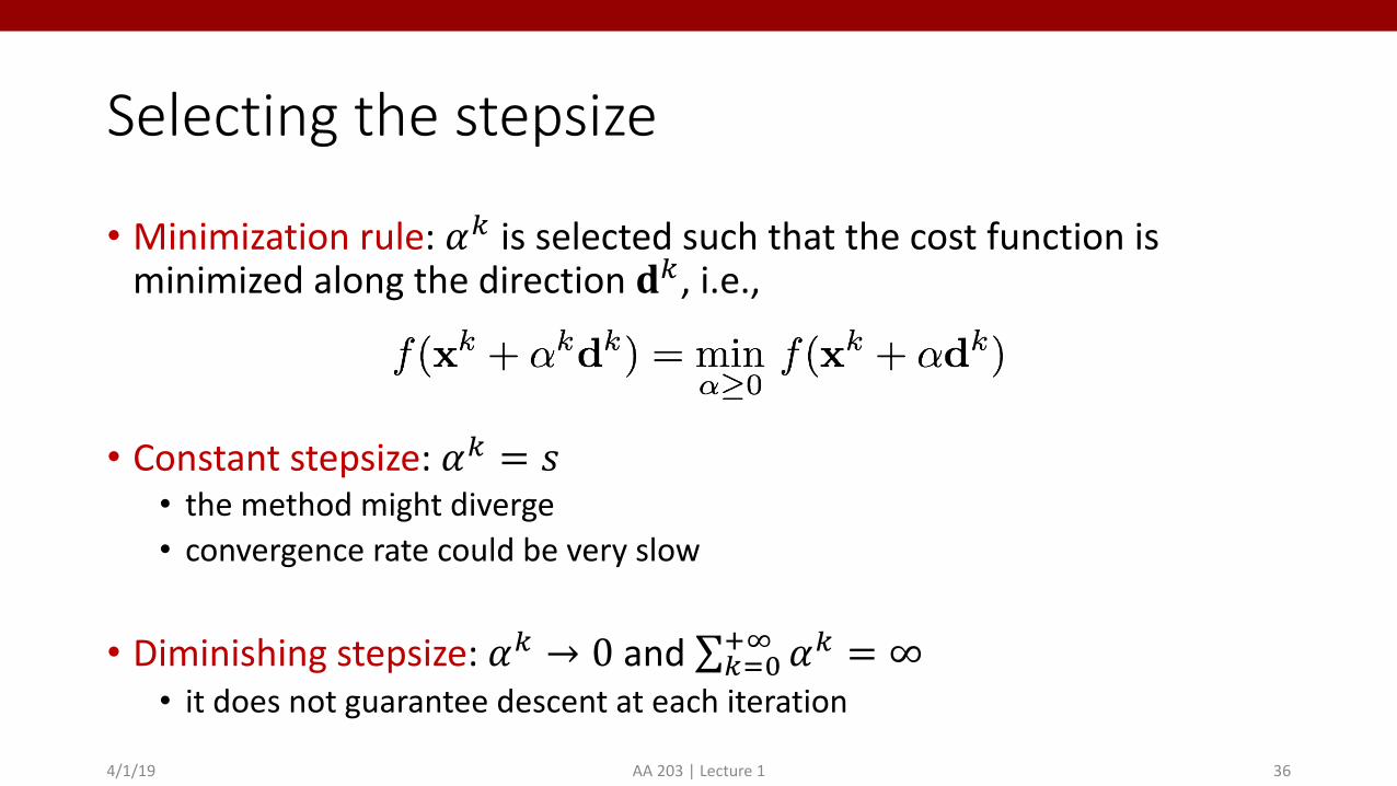
Selecting the stepsize

• Minimization rule: !" is selected such that the cost function is minimized along the direction #", i.e.,

• Constant stepsize: !" = %• the method might diverge• convergence rate could be very slow

• Diminishing stepsize: !" → 0 and ∑")*+, !" = ∞• it does not guarantee descent at each iteration

4/1/19 AA 203 | Lecture 1 36

Discussion

Aspects:• convergence (to stationary points)• termination criteria • convergence rate

Non-derivative methods, e.g., • coordinate descent

4/1/19 AA 203 | Lecture 1 37

Next time

4/1/19 AA 203 | Lecture 1 38

Constrained non-linear optimization