aalborg university department of computer science -...
TRANSCRIPT

Aalborg UniversityDepartment of Computer Science
Fredrik Bajersvej 7 DK-9220 Aalborg East
Title
Grid Information Service with
Self-Organized Network and Information Traveling
Project group:
SSE4 B2-201
Members:
Baolong Feng
Huong Duong Uong
Tuan Anh Nguyen
Project period:
1-Feb-2006 to 15-June-2006
Number of pages:
103
Supervisor:
Josva Kleist
ABSTRACT:With respect to scalability, fault-tolerance
and flexibility requirements, we proposed
a novel architecture of Grid Informa-
tion Service. Two outstanding features
of this architecture are nodes applying
Optimized Link State Routing Protocol
(OLSR) to self-organize network structure
and resource information traveling around
in terms of its validity.
The architecture was implemented and
the system is well functioning. It was con-
firmed that using OLSR the system is able
to automatically build up and then main-
tain the network as expected, and the net-
work structure is fault-tolerant and flexi-
ble. Many experiments have been done re-
garding the performance, and the results
show that the system appears to be scal-
able.
Aalborg, June 2006

2
This project is done by SSE4-group B2-201
Baolong Feng
Huong Duong Uong
Tuan Anh Nguyen
Contents
1 Introduction 7
1.1 Introduction to computational grid . . . . . . . . . . . . . . . . . . . . . . . 7
1.2 The anatomy of computational grid . . . . . . . . . . . . . . . . . . . . . . . 8
1.3 Grid Information Service . . . . . . . . . . . . . . . . . . . . . . . . . . . . . 10
1.4 Our work . . . . . . . . . . . . . . . . . . . . . . . . . . . . . . . . . . . . . 11
2 Implementation 13
2.1 Introduction . . . . . . . . . . . . . . . . . . . . . . . . . . . . . . . . . . . . 13
2.1.1 Introduction to OLSR . . . . . . . . . . . . . . . . . . . . . . . . . . 13
2.1.2 Introduction to Twisted . . . . . . . . . . . . . . . . . . . . . . . . . 16
2.2 Components . . . . . . . . . . . . . . . . . . . . . . . . . . . . . . . . . . . . 20
2.2.1 MultiConsumer . . . . . . . . . . . . . . . . . . . . . . . . . . . . . . 20
2.2.2 MultiProducer . . . . . . . . . . . . . . . . . . . . . . . . . . . . . . . 20
2.2.3 ISNode . . . . . . . . . . . . . . . . . . . . . . . . . . . . . . . . . . . 21
2.3 Working procedure . . . . . . . . . . . . . . . . . . . . . . . . . . . . . . . . 21
2.3.1 Self-organized Network . . . . . . . . . . . . . . . . . . . . . . . . . . 21
2.3.2 Resource information and query storage . . . . . . . . . . . . . . . . 22
2.3.3 Information traveling . . . . . . . . . . . . . . . . . . . . . . . . . . . 27
2.3.4 Query answering . . . . . . . . . . . . . . . . . . . . . . . . . . . . . 28
2.3.5 Producer and Consumer membership maintenance . . . . . . . . . . . 31
3

CONTENTS 4
2.3.6 Time synchronizing . . . . . . . . . . . . . . . . . . . . . . . . . . . . 32
2.3.7 Security . . . . . . . . . . . . . . . . . . . . . . . . . . . . . . . . . . 32
2.3.8 Virtual Organization . . . . . . . . . . . . . . . . . . . . . . . . . . . 32
2.4 Performance data measurement . . . . . . . . . . . . . . . . . . . . . . . . . 33
2.4.1 Query anwsering . . . . . . . . . . . . . . . . . . . . . . . . . . . . . 33
2.4.2 Information traveling . . . . . . . . . . . . . . . . . . . . . . . . . . . 33
2.5 Summary . . . . . . . . . . . . . . . . . . . . . . . . . . . . . . . . . . . . . 34
3 Design of experiments 35
3.1 Experimental environment . . . . . . . . . . . . . . . . . . . . . . . . . . . . 35
3.2 Parameters for experiments . . . . . . . . . . . . . . . . . . . . . . . . . . . 36
3.2.1 Parameters for ISNode . . . . . . . . . . . . . . . . . . . . . . . . . . 36
3.2.2 Parameters for Producer . . . . . . . . . . . . . . . . . . . . . . . . . 37
3.2.3 Parameters for Consumer . . . . . . . . . . . . . . . . . . . . . . . . 38
3.2.4 Workload . . . . . . . . . . . . . . . . . . . . . . . . . . . . . . . . . 40
3.2.5 Time To Live (TTL) . . . . . . . . . . . . . . . . . . . . . . . . . . . 42
3.3 Capacity . . . . . . . . . . . . . . . . . . . . . . . . . . . . . . . . . . . . . . 43
3.4 Availability . . . . . . . . . . . . . . . . . . . . . . . . . . . . . . . . . . . . 45
3.5 Scalability . . . . . . . . . . . . . . . . . . . . . . . . . . . . . . . . . . . . . 46
3.5.1 Query answering performance . . . . . . . . . . . . . . . . . . . . . . 47
3.5.2 Information traveling performance . . . . . . . . . . . . . . . . . . . . 47
3.5.3 Experiment with 6 nodes . . . . . . . . . . . . . . . . . . . . . . . . . 48
3.5.4 Experiment with 8 nodes . . . . . . . . . . . . . . . . . . . . . . . . . 50
3.5.5 Experiment with 15 nodes . . . . . . . . . . . . . . . . . . . . . . . . 51
3.5.6 Experiments with 24 nodes . . . . . . . . . . . . . . . . . . . . . . . . 52
3.5.7 Experiments with 36 nodes . . . . . . . . . . . . . . . . . . . . . . . . 54
3.6 Summary . . . . . . . . . . . . . . . . . . . . . . . . . . . . . . . . . . . . . 55
CONTENTS 5
4 Results 56
4.1 Capacity . . . . . . . . . . . . . . . . . . . . . . . . . . . . . . . . . . . . . . 56
4.1.1 Capacity for all experiments . . . . . . . . . . . . . . . . . . . . . . . 57
4.2 Availability . . . . . . . . . . . . . . . . . . . . . . . . . . . . . . . . . . . . 58
4.3 Scalability . . . . . . . . . . . . . . . . . . . . . . . . . . . . . . . . . . . . . 60
4.3.1 Experiment with 6 nodes . . . . . . . . . . . . . . . . . . . . . . . . . 60
4.3.2 Experiment with 8 nodes . . . . . . . . . . . . . . . . . . . . . . . . . 64
4.3.3 Experiment with 15 nodes . . . . . . . . . . . . . . . . . . . . . . . . 67
4.3.4 Experiments with 24 nodes . . . . . . . . . . . . . . . . . . . . . . . . 70
4.3.5 Experiments with 36 nodes . . . . . . . . . . . . . . . . . . . . . . . . 74
4.4 Summary . . . . . . . . . . . . . . . . . . . . . . . . . . . . . . . . . . . . . 79
5 Analysis 80
5.1 Scalability . . . . . . . . . . . . . . . . . . . . . . . . . . . . . . . . . . . . . 80
5.2 Information traveling . . . . . . . . . . . . . . . . . . . . . . . . . . . . . . . 82
5.3 Design of more experiments . . . . . . . . . . . . . . . . . . . . . . . . . . . 82
5.3.1 Experiment of 24 nodes with net backbone . . . . . . . . . . . . . . . 82
5.3.2 Experiment of 24 nodes with line backbone . . . . . . . . . . . . . . . 83
5.3.3 Experiment of 36 nodes with 5-node backbone . . . . . . . . . . . . . 84
5.4 Summary . . . . . . . . . . . . . . . . . . . . . . . . . . . . . . . . . . . . . 84
6 More experiments 85
6.1 Compare 24 nodes between ring and net backbone . . . . . . . . . . . . . . . 85
6.1.1 Query answering performance . . . . . . . . . . . . . . . . . . . . . . 86
6.1.2 Information traveling performance . . . . . . . . . . . . . . . . . . . . 86
6.2 Compare 24 nodes between ring and line backbone . . . . . . . . . . . . . . 87
6.2.1 Query answering performance . . . . . . . . . . . . . . . . . . . . . . 87

CONTENTS 6
6.2.2 Information traveling performance . . . . . . . . . . . . . . . . . . . . 88
6.3 Compare 36 nodes between 6 and 5 nodes ring backbone . . . . . . . . . . . 88
6.3.1 Query answering performance . . . . . . . . . . . . . . . . . . . . . . 90
6.3.2 Information traveling performance . . . . . . . . . . . . . . . . . . . . 90
6.4 Analysis . . . . . . . . . . . . . . . . . . . . . . . . . . . . . . . . . . . . . . 91
6.5 Summary . . . . . . . . . . . . . . . . . . . . . . . . . . . . . . . . . . . . . 91
7 Related work 92
7.1 Compare with MDS . . . . . . . . . . . . . . . . . . . . . . . . . . . . . . . . 92
7.2 Other peer-to-peer approaches . . . . . . . . . . . . . . . . . . . . . . . . . . 94
7.2.1 A peer-to-peer information service for Grid . . . . . . . . . . . . . . . 94
7.2.2 Super-peer network . . . . . . . . . . . . . . . . . . . . . . . . . . . . 95
7.2.3 Evaluation . . . . . . . . . . . . . . . . . . . . . . . . . . . . . . . . . 95
7.3 Summary . . . . . . . . . . . . . . . . . . . . . . . . . . . . . . . . . . . . . 97
8 Conclusion and Future work 98
8.1 Compare with MDS . . . . . . . . . . . . . . . . . . . . . . . . . . . . . . . . 98
8.2 New query answering mechanism . . . . . . . . . . . . . . . . . . . . . . . . 99
8.3 Finding out the limit . . . . . . . . . . . . . . . . . . . . . . . . . . . . . . . 100

Chapter 1
Introduction
Over the last ten years, enormous effort has been made by many scientists and researchers
on a very active scientific area, Computational Grid. To date, significant achievements
have been obtained, but there is still a large amount of work to do in this area.
We are very interested in computational grid, and have been working on Grid Information
Service (GIS) for two semesters. This report is the documentation of the second semester
and our Master thesis. As a beginning, we introduce the fundamental concept and the
anatomy of computational grid in Section 1.1 and Section 1.2, respectively. We locate our
concern on GIS, which is an important component of computational grid, as described in
Section 1.3. We also present our work that was done last semester and that will be done in
this semester in Section 1.4.
1.1 Introduction to computational grid
To date, computers have been widely used in industry, scientific research and daily life. It
is predictable that in the next decade, people will keep seeking for more and more compu-
tational power for a large number of applications that are significant to human being and
consume huge computational power, such as weather forecast, meteorology research, physical
simulation and so on. People always feel the inadequacy of computational environment for
such computationally sophisticated purposes, even though the performance of today’s PC
has been highly improved using chips produced by vendors such as Intel and AMD, while
IBM and SUN have been continuously working hard on supercomputers.
Computational grid is an infrastructure that provides high-end computational capabilities
7

CHAPTER 1. INTRODUCTION 8
by increasing demand-driven access to computational power, use of idle capacity, and sharing
of computational results. In [15], the definition of computational grid is introduced:
“A computational grid is a hardware and software infrastructure that provides dependable,
consistent, pervasive, and inexpensive access to high-end computational capabilities.”
The hardware infrastructure of computational grid interconnects large-scale resources re-
gardless of the location, and the software infrastructure of computational grid provides the
functionalities to monitor and control the computational environment.
Dependable means that users obtain assurances that they will receive predictable, sustained
and often high levels of performance.
Consistent means that standard, accessible via standard interfaces, and operating with stan-
dard parameters.
Pervasive means that users are able to count on services always being available.
Computational grid is able to be used for a large number of applications such as distrib-
uted supercomputing, high-throughput computing, on-demand computing, data-intensive
computing, collaborative computing and so on.
1.2 The anatomy of computational grid
Figure 1.1: Grid architecture
The grid concept is indeed motivated by a real and specific problem named grid problem, as
CHAPTER 1. INTRODUCTION 9
defined in [16]:
“The real and specific problem that underlies the grid concept is coordinated resource sharing
and problem solving in dynamic, multi-institutional virtual organizations (VO).”
In [16], a grid architecture is presented. This grid architecture is a protocol architecture
with protocols defining the basic mechanisms by which users and resources negotiate, estab-
lish, manage and exploit sharing relationship. This architecture is an extensible, open and
layered architecture identifying requirements of general classes of components, as shown in
Figure 1.1. Components within each layer build on capabilities and behaviors provided by
any lower layer.
The Fabric layer provides the resources to which shared access is mediated by grid protocol,
such as computational resources, storage systems, catalogs, network resources, sensors and
so on. The fabric components implement the local, resource-specific operations on specific
resources, including enquiry mechanisms permitting discovery of the structure, state and
capabilities of resources, and resource management mechanisms providing the control of
delivered quality of service.
The Connectivity layer defines core communication and authentication protocols required
for grid-specific network transactions. Communication protocols enable the exchange of data
between Fabric layer resources. Authentication protocols build on communication services
to provide secure mechanisms for verifying the identity of users and resources.
The Resource layer builds on Connectivity layer communication and authentication proto-
cols to define protocols for the secure negotiation, initiation, monitoring, control, accounting
and payment of sharing operations on individual resources. Resource layer implementations
of these protocols call Fabric layer functions to access and control local resources. Two
primary classes of Resource layer protocols are: information protocols, which are used to
obtain information about the structure and state of a resource, and management protocols,
which are used to negotiate access to a shared resource.
The Collective layer contains protocols and services that are global in nature and capture
interactions across collections of resources, compared with Resource layer that is focused
on interactions with a single resource. Collective components build on Resource layer and
Connectivity layer, and implement a wide variety of behaviors on the resources, for example:
• Directory services allow VO participants to discover the existence and/or properties
of VO resources. A directory service may allow its users to query for resources by name
and/or by attributes such as type, availability, or load.

CHAPTER 1. INTRODUCTION 10
• Co-allocation, scheduling and brokering services allow VO participants to request the
allocation of one or more resources for a specific purpose and the scheduling of tasks
on the appropriate resources.
• Monitoring and diagnostics services support the monitoring of VO resources for failure,
adversarial attack, overload, and so on.
• Data replication services support the management of VO storage resources.
• Community authorization servers enforce community policies governing resource ac-
cess, generating capabilities that community members can use to access community
resources.
• Community accounting and payment services gather resource usage information for
the purpose of accounting, payment, and/or limiting of resource usage by community
members.
Application layer comprises the user applications that operate within a VO environment.
Applications are constructed in terms of, and by calling upon, services defined at any lower
layer.
An example [16] illustrates how this grid architecture functions in practice. Table 1.1 shows
the services that may be used to implement the sharing of spare computing cycles to run
ray tracing computations.
Ray TracingCollective (application-specific) Checkpointing, job management, failover, stagingCollective (generic) Resource discovery, resource brokering, system monitoring, com-
munity authorization, certificate revocationResource Access to computation; access to data; access to information
about system structure, state, performance.Connectivity Communication (IP), service discovery (DNS), authentication, au-
thorization, delegationFabric Storage systems, computers, networks, code repositories, catalogs
Table 1.1: The grid services used to construct the ray tracing application
1.3 Grid Information Service
In computational grid, the discovery, characterization and monitoring of resources, services
and computations are challenging due to the considerable diversity, large numbers, dynamic

CHAPTER 1. INTRODUCTION 11
behavior and geographical distribution of the entities in which a user might be interested. As
a result, information services are a vital part of any grid software infrastructure, providing
fundamental mechanisms for discovery and monitoring and thus for planning and adapting
application behavior [12].
A few examples illustrate the wide range of applications that rely on GISs, which indicates
the importance of GIS [12].
• A service discovery service records the identity and essential characteristics of services
available to community members. Such a discovery service might enable a user to
determine that a new site has 100 new CPUs available for approved use. GIS provides
availability information of resources to service discovery service.
• A superscheduler routes computational requests to the best available computer in a grid
containing multiple high-end computers, where best can encompass issues of architec-
ture, installed software, performance, availability, and policy. GIS provides resource
information of computers, such as system configuration, instantaneous load and pre-
diction of future availability, to superscheduler.
• A replica selection service within a data grid responds to requests for the best copy
of files that are replicated on multiple storage systems. GIS provides resource infor-
mation of storage systems and networks, such as system configuration, instantaneous
performance and predictions, to replica selection service.
1.4 Our work
Last semester, we deeply studied computational grid and did a broad survey on GIS [14].
Through the survey, we realized that the existing GISs including MDS [12] and R-GMA [11]
are unable to work effectively and efficiently in a huge grid with respect to the requirements
of scalability, fault-tolerance and flexibility. As a result, we proposed a new GIS with self-
organized network and information traveling. We designed, implemented and tested only
the Optimized Link State Routing Protocol (OLSR) (see Section 2.1.1) subsystem, which is
a distributed program applying OLSR to self-organize the network structure. The testing
results indicate that the program with suitable configuration is able to automatically build
up and then maintain the network as expected.
In this semester, we will complete the implementation of our GIS, and then evaluate the
implementation by doing experiments. The rest of this report will be described as follow.

CHAPTER 1. INTRODUCTION 12
Chapter 2 will describe the implementation of our system. Three main focuses, namely the
components, the working procedures and performance data measurement, are presented one
by one.
In Chapter 3, first we introduce the environment for our experiments. Second, all important
parameters are explained. Three main aspects, namely capacity, availability and scalability,
are described, respectively in Section 3.3, 3.4 and 3.5.
Chapter 4 will present the result of our experiment regarding capacity, availability and
scalability.
In Chapter 5, we analyze the results as described in Chapter 4. The main focuses are about
scalability and information traveling. After that, we design new experiments to observe more
behaviors of our system.
Chapter 6 will compare the results with different network sizes and shapes, namely compare
our system of ring backbone with line or net backbone. We also present the comparison
when the size of ring backbone is reduced.
Chapter 7 presents related work. We will make comparison with MDS and also introduce
two other approaches that also use peer-to-peer to develop GIS.
In Chapter 8, we present the conclusion and propose our future work.

Chapter 2
Implementation
This chapter mainly describes how we build up the GIS from our proposal. In addition,
Optimized Link State Routing Protocol (OLSR) and Twisted are introduced.
2.1 Introduction
2.1.1 Introduction to OLSR
In this section, we briefly introduce OLSR, which was developed for mobile ad hoc network
(MANET) and documented in the Request For Comment (RFC) 3626 [3]. The RFC 3626
defines the core functionality and a set of additional functions. The key point of OLSR is
multipoint relays (MPRs), which will be presented in Section 2.1.1.2. We also present a
short description of the core functionality in Section 2.1.1.3.
2.1.1.1 Overview of OLSR
OLSR is a proactive routing protocol, and it inherits the stability of the classic link state
algorithm and has the advantage of having routes immediately available when needed. OLSR
is an optimization over the classical link state protocol, tailored for mobile ad hoc networks.
The reason why we utilize OLSR in our proposal is that OLSR has two features that are
very valuable for building a GIS. These two features are quick response to network changes
and optimized information flooding.
In reality, a GIS is always built on a large and unstable computer network. Nodes of a
13

CHAPTER 2. IMPLEMENTATION 14
GIS might crash from time to time. As a result, quick response to network changes is very
important to a good GIS.
In OLSR, only nodes, selected to be MPRs (see Section 2.1.1.2), are responsible for for-
warding control traffic, intended for diffusion into the entire network. Thus OLSR highly
optimizes the flooding of information among nodes on the network. This outstanding ap-
proach is very meaningful to a GIS. In a grid system, resource information is geographically
distributed on the network, and a GIS should efficiently provide resource information. This
leads to frequent information exchanges among the nodes of a GIS. Using optimized infor-
mation flooding will highly reduce unnecessary information transmission inside a GIS.
2.1.1.2 Mutipoint relays
The basic idea of multipoint relays is to minimize the overhead of flooding messages in the
network by reducing redundant retransmissions.
Each node in the network selects a set of nodes in its symmetric 1-hop neighbors which
may retransmit its messages. This set is called the Multipoint Relay (MPR) set of that node.
This set must cover all symmetric strict 2-hop neighbors. This means that the MPR
Set of node A, denoted as MPR(A), is a subset of the set of the symmetric 1-hop neighbors
of A, such that every symmetric strict 2-hop neighbor of A must have at least a symmetric
link to a node in MPR(A).
The terms symmetric 1-hop neighbor and symmetric strict 2-hop neighbor are definitely
defined in [3]. Brief descriptions are as follows. The symmetric 1-hop neighborhood of any
node X is the set of nodes which have at least one symmetric link1 to X. The symmetric
strict 2-hop neighborhood of X is the set of nodes, excluding X itself and its neighbors,
which have a symmetric link to some symmetric 1-hop neighbor, with willingness different
of WILL NEVER2, of X.
Figure 2.1 illustrates that node A selects nodes {M1,M2,M3,M4} as its MPR Set. All 2-hop
neighbors {B1,B2,...,B8} of A can be reached through its MPRs. Node N1 and N2 will not
retransmit traffic from A because they are not MPRs of A. N1 is not a MPR due to the fact
that it has no links to symmetric strict 2-hop neighbors of A. N2 is not a MPR because it
does not have a symmetric link to symmetric strict 2-hop neighbors.
1Symmetric link: a verified bi-directional link between two OLSR interfaces.2A node with willingness WILL NEVER must never be selected as MPR by any node.

CHAPTER 2. IMPLEMENTATION 15
Figure 2.1: Muiltipoint Relays
2.1.1.3 Core functioning
Core functioning is made up of the following functions:
Packet Format and Forwarding: This function provides specification of the packet format
for OLSR communication. This also provides processing and forwarding messages mecha-
nism.
Link Sensing: The purpose of this function is to establish the links over the nodes. The
information related to links is stored in local link information base. This function can be
accomplished through periodic emission of HELLO message3.
Neighbor Detection: This function maintains the neighborhood information base. By
having association with Link Sensing, it can populate the Neighbor Set4, 2-hop Neighbor
Set5 and MPR Set.
MPR Selection and Signaling: The objective of MPR selection is for a node to select
a subset of its neighbors such that a broadcast message, retransmitted by these selected
neighbors, will be received by all nodes 2 hops away. The information required to perform
3HELLO message is transmitted only between two neighboring nodes. Its format and generation isdetailedly described in [3].
4Neighbor Set is a set of records that a node makes to describes all neighbors.52-hop Neighbor Set is a set of records that a node makes to describe symmetric (and, since MPR links
by definition are also symmetric, thereby also MPR) links between its neighbors and the symmetric 2-hopneighborhood.

CHAPTER 2. IMPLEMENTATION 16
this calculation is provided through periodic exchange of HELLO message.
Topology Discovery: This function is performed through exchanging topology controll
message. The purpose is to provide sufficient link-state information for each node in order
to have a route calculation.
Route Calculation: This function computes the routing table for each node. This is based
on given link-state information.
Since the optimized information flooding approach is of interest to our proposal, only four
core functions are necessary: Packet Format and Forwarding, Link Sensing, Neighbor De-
tection, MPR Selection and Signaling.
2.1.2 Introduction to Twisted
Twisted is an open source networking framework, which is implemented in Python and devel-
oped by Twisted Matrix Laboratories [8]. Twisted framework provides rich APIs at multiple
levels of abstraction to facilitate different kinds of network programming and different plat-
forms. With Twisted’s event-based and asynchronous framework, we can work with multiple
network connections at once within a single thread.
Figure 2.2: High-level overview of Twisted

CHAPTER 2. IMPLEMENTATION 17
We choose Perspective Broker (one of core elements in Twisted that provides Remote Method
Call (RPC) and supports exchanging serialized Python objects) to implement the commu-
nication mechanism in our program. Figure 2.2 demonstrates the high-level overview of
Twisted.
As described in [7], the Perspective Broker (abbreviated PB) is based upon two central
concepts:
• serialization: PB provides the mechanism that an object can be serialized into into a
chunk of bytes, and this serialized object will be able to be sent to the other side.
• Remote Method Call : PB also provides the mechanism that a local object can have
methods that can be invoked remotely.
Due to the fact that our network structure is peer-to-peer, each node is both acting as server
and client. Being a server, each node simply inherits pb.Root class in order to support referen-
cable objects. To define a method that can be invoked remotely, the method name must begin
with remote prefix. Being a client, each node makes a connection to the server and requests
the reference of the server’s object. When the connection has been made, the client side can
invoke remote methods on the server by calling remote obj.callRemote("name of remote method")
(remote obj is the reference to the remote object.).
Figure 2.3 shows the fragments of the code which are implemented for the server side by
using PB. ISNodeHandler is a class that provides all methods that the other nodes can call
remotely. After running method run, a node will start a service that listens on the server port
and dispatches the remote method calls to the appropriate methods. The six remote methods
such as remote is static unit existed and so on are invoked by Producers or other nodes to
transfer resource information.
Figure 2.4 shows the fragments of the code which are implemented for the client side by using
PB. Class MakeConnection is used to make the connection to the server. When the connection
is made, the reference to the remote object is stored. Afterward method publish static unit
will be invoked and the method remote is static unit existed in the server side will be called
through the function call remote obj.callRemote("is static unit existed",...).
Resource information is transferred among nodes by using Python List. There is no need
to serialize Python List. However, serialization is necessary for HELLO messages, which are
periodically exchanged between two neighboring nodes to maintain network structure. Each
HELLO message is actually an object that will be passed as an argument in a RPC when
the sender is acting as client.

CHAPTER 2. IMPLEMENTATION 18
from twisted.spread import pb, jelly
from twisted.internet import reactor, defer
class ISNodeHandler(pb.Root):
# remote method is named with remote_ prefix
def remote_is_static_unit_existed(self, ...):
#method body
...
def remote_is_dynamic_unit_existed(self, ...):
...
def remote_add_static_unit(self, ...):
...
def remote_update_static_unit(self, ...):
...
def remote_add_dynamic_unit(self, ...):
...
def remote_update_dynamic_unit(self, ...):
...
# start listening on server_port
def run(self):
reactor.listenTCP(server_port, pb.PBServerFactory(self))
Figure 2.3: Server side using Perspective Broker
class MakeConnection:
def set_up_connection(self):
...
# make a connection
factory = pb.PBClientFactory()
# get referenceable object
factory.getRootObject().addCallbacks(self.connection_made, ...)
reactor.connectTCP(...)
...
def connection_made(self, remote_obj):
self.root.remote_objs.append([self.neighbor, remote_obj])
...
class StaticHandler:
def publish_static_unit(self):
...
self.remote_obj.callRemote("is_static_unit_existed", ...).addCallbacks(...)
Figure 2.4: Client side using Perspective Broker

CHAPTER 2. IMPLEMENTATION 19
class HelloMessage:
# the class body
...
class CopyableHelloMessage(HelloMessage, pb.Copyable):
# the class body
...
class ReceivableHelloMessage(pb.RemoteCopy, HelloMessage):
# the class body
...
def init_copyable_hello_msg():
pb.setUnjellyableForClass(CopyableHelloMessage, ReceivableHelloMessage)
Figure 2.5: Serialization using Perspective Broker
In order to provide a mechanism for serializing the HelloMessage objects, the following steps
have to be done:
1. A normal class HelloMessage is defined, but the objects of this class can not be passed
as an argument of a RPC. As a result, we have to define a new class that inherits class
HelloMessage as described in step 2.
2. Class CopyableHelloMessage is defined to inherit HelloMessage and pb.Copyable provided
by Perspective Broker. The objects of this new class can be passed as an argument
of a RPC. Therefore, whenever a node wants to transfer the HelloMessage object, an
instance of class CopyableHelloMessage should be created.
3. In the other node, when receiving the CopyableHelloMessage object, an instance of
class ReceivableHelloMessage will be created. Class ReceivableHelloMessage inherits
HelloMessage and pb.RemoteCopy. The objects of this class are used to receive the ob-
jects of class CopyableHelloMessage. The mapping between class CopyableHelloMessage
and ReceivableHelloMessage is described in step 4.
4. Function init copyable hello msg will be used to set up the mapping between two
classes: CopyableHelloMessage and ReceivableHelloMessage. This method should be
called before transferring the CopyableHelloMessage object as an argument of a RPC.
Figure 2.5 shows the fragments of 4 steps mentioned above.

CHAPTER 2. IMPLEMENTATION 20
2.2 Components
In our proposal, the GIS has three components, namely Consumer, Producer and IS node,
as depicted in Figure 2.6.
Figure 2.6: Components of the GIS
For the purpose of experiments, we write three programs, MultiConsumer, MultiProducer
and ISNode, to implement three components of our GIS.
2.2.1 MultiConsumer
MultiConsumer is a program that simulates a predefined number of Consumers. A Con-
sumer periodically creates and sends queries to local IS node6, and then retrieves matched
information from local IS node.
2.2.2 MultiProducer
MultiProducer is a program that simulates a predefined number of Producers. A Producer
simulates generating resource information that belongs to a site, and periodically publishes
resource information of this site to local IS node7. We assume there is only one resource
6A local IS node of a Consumer is the IS node that is manually assigned to a Consumer and contactedby this Consumer by default.
7A local IS node of a Producer is the IS node that is manually assigned to a Producer and contacted bythis Producer by default.
CHAPTER 2. IMPLEMENTATION 21
at each site, so the resource information of a site is actually that of a single cluster or
supercomputer.
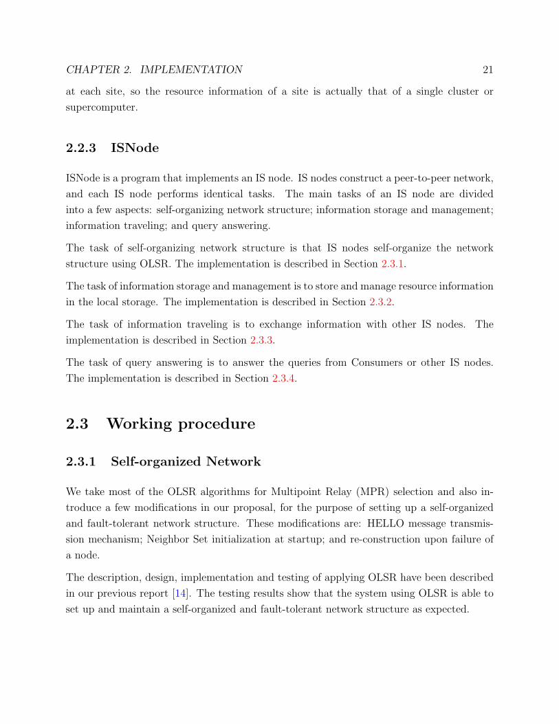
2.2.3 ISNode
ISNode is a program that implements an IS node. IS nodes construct a peer-to-peer network,
and each IS node performs identical tasks. The main tasks of an IS node are divided
into a few aspects: self-organizing network structure; information storage and management;
information traveling; and query answering.
The task of self-organizing network structure is that IS nodes self-organize the network
structure using OLSR. The implementation is described in Section 2.3.1.
The task of information storage and management is to store and manage resource information
in the local storage. The implementation is described in Section 2.3.2.
The task of information traveling is to exchange information with other IS nodes. The
implementation is described in Section 2.3.3.
The task of query answering is to answer the queries from Consumers or other IS nodes.
The implementation is described in Section 2.3.4.
2.3 Working procedure
2.3.1 Self-organized Network
We take most of the OLSR algorithms for Multipoint Relay (MPR) selection and also in-
troduce a few modifications in our proposal, for the purpose of setting up a self-organized
and fault-tolerant network structure. These modifications are: HELLO message transmis-
sion mechanism; Neighbor Set initialization at startup; and re-construction upon failure of
a node.
The description, design, implementation and testing of applying OLSR have been described
in our previous report [14]. The testing results show that the system using OLSR is able to
set up and maintain a self-organized and fault-tolerant network structure as expected.

CHAPTER 2. IMPLEMENTATION 22
2.3.2 Resource information and query storage
In this section, we introduce what and how resource information is stored in our GIS imple-
mentation, in Section 2.3.2.1 and 2.3.2.2 respectively. In addition, we present how queries
are stored in Section 2.3.2.3.
2.3.2.1 Introduction to resource information
In our GIS implementation, MultiProducer simulates a predefined number of Producers. A
Producer simulates generating resource information that belongs to a site. For the purpose
of simulation, we studied NorduGrid information system [17], and then decided to take
most of the attributes regarding a cluster defined in NorduGrid information system. These
attributes describe the static and dynamic properties of a cluster.
Tables 2.1-2.5 show the attributes that are chosen. For simplicity, we choose only the at-
tributes regarding 3 categories of resource information, namely Cluster, Queue and Job
information. Detailed descriptions about these attributes are presented in the paper of
NorduGrid information system [10].
The Cluster and Queue information are split into 2 sub-categories, namely static and dy-
namic, due to the fact that some attributes are changing more frequently than others. The
Job information is always considered as dynamic. By splitting into 2 sub-categories, more
frequently changing attributes are being updated as needed, while others can hold for a
longer time. As a result of splitting, we have (i) dynamic and static Cluster information; (ii)
dynamic and static Queue information; and (iii) Job information.
In addition, we introduce a few new attributes into dynamic and static Cluster informa-
tion for the purpose of information traveling, as shown at the end of Table 2.1. For a
piece of resource information, STATIC TTL defines how far it can travel (hops); STA-
TIC VALIDFROM and STATIC VALIDTO define when it was generated and when it will
be expired respectively, and expired information will be removed; STATIC ORIGINATOR is
the address of this information’s Producer’s local IS node; STATIC SENDER is the address
of the sender IS node from which this piece of resource information came. The counterparts
at the end of Table 2.2 have the similar meanings.
The size of the resource information generated by a Producer on behalf of a cluster is about
7800 Bytes (We have this number by dumping resource information of a cluster into a file).

CHAPTER 2. IMPLEMENTATION 23
Item
STATIC CLUSTER NAME
CLUSTER ALIASNAME
CLUSTER CONTACTSTRING
CLUSTER SUPPORT
CLUSTER LOCATION
CLUSTER OWNER
CLUSTER ISSUERCA
CLUSTER LRMS TYPE
CLUSTER LRMS VERSION
CLUSTER LRMS CONFIG
CLUSTER HOMOGENEITY
CLUSTER ARCHITECTURE
CLUSTER OPSYS
CLUSTER NODECPU
CLUSTER NODEMEMORY
CLUSTER TOTALCPUS
CLUSTER CPUDISTRIBUTION
CLUSTER SESSIONDIR TOTAL
CLUSTER CACHE TOTAL
CLUSTER RUNTIMEENVIRONMENT
CLUSTER LOCALSE
CLUSTER MIDDLEWARE
CLUSTER NODEACCESS
CLUSTER COMMENT
STATIC TTL
STATIC VALIDFROM
STATIC VALIDTO
STATIC ORIGINATOR
STATIC SENDER
Table 2.1: Static Cluster information
Item
DYNAMIC CLUSTER NAME
CLUSTER SESSIONDIR FREE
CLUSTER CACHE FREE
CLUSTER TOTALJOBS
CLUSTER USEDCPUS
CLUSTER QUEUEDJOBS
DYNAMIC TTL
DYNAMIC VALIDFROM
DYNAMIC VALIDTO
DYNAMIC ORIGINATOR
DYNAMIC SENDER
Table 2.2: Dynamic Cluster information

CHAPTER 2. IMPLEMENTATION 24
Item
STATIC QUEUE CLUSTER NAME
QUEUE NAME
QUEUE MAXRUNNING
QUEUE MAXCPUTIME
QUEUE DEFAULTCPUTIME
QUEUE SCHEDULINGPOLICY
QUEUE TOTALCPUS
QUEUE NODECPU
QUEUE NODEMEMORY
QUEUE ARCHITECTURE
QUEUE OPSYS
Table 2.3: Static Queue information
Item
DYNAMIC QUEUE CLUSTER NAME
QUEUE NAME
QUEUE STATUS
QUEUE GRIDRUNNING
QUEUE GRIDQUEUED
Table 2.4: Dynamic Queue information
Item
JOB EXECCLUSTER
JOB EXECQUEUE
JOB GLOBALID
JOB GLOBALOWNER
JOB JOBNAME
JOB SUBMISSIONTIME
JOB STATUS
JOB QUEUERANK
JOB CPUCOUNT
JOB STDOUT
JOB STDERR
JOB GMLOG
JOB RUNTIMEENVIRONMENT
JOB SUBMISSIONUI
JOB CLIENTSOFTWARE
JOB PROXYEXPIRATIONTIME
Table 2.5: Job information

CHAPTER 2. IMPLEMENTATION 25
2.3.2.2 Resource information data model
In previous report, we mentioned that the resource information data model of our GIS uses
XML format. However, using XML format requires a lot of operations to convert back and
forth and to retrieve the content of resource information. If we apply the XML data model
in our GIS implementation, the performance might not be as good as expected. As a result,
we decided to drop the idea of using XML in our GIS implementation.
Another solution has been examined, which is using the relational database as data model.
In the very beginning of this semester, we tried to use a relational database system, MySQL
[2]. Unfortunately, the result showed that the relational database is not suitable for our
implementation. The reason is because in our implementation, there is too much information
exchanging among IS nodes. Because information is being added or modified frequently in
each IS node, a huge number of database operations are required. We discovered that using
MySQL the performance was not good. We also tried one in-memory relational database
system, Gadfly [1], but the performance was even worse.
We choose to apply Python dictionary [5] for storing data, and thus resource information
data is kept in main memory. Python dictionaries are created by placing a comma-separated
list of key: value pairs within braces, for example: {’jack’: 4098, ’mike: 4127}. The following
list is a brief summary of Python dictionary characteristics:
• A dictionary is an unordered collection of objects.
• Values are accessed using a key rather than by using an ordinal numeric index.
• A dictionary can shrink or grow as needed.
• The contents of dictionaries can be modified.
• Dictionaries can be nested.
• Dictionaries are not sequences. Sequence operations such as slice cannot be used with
dictionaries.
Specifically, the Python dictionary is used for storing resource information published from
Producers and from other IS nodes. The size of the resource information generated by a
Producer on behalf of a site is about 7800 Bytes, so storing resource information data in
memory is acceptable for current computers that usually contain 512M Bytes memory or
even more.

CHAPTER 2. IMPLEMENTATION 26
self.staticcluster = {}
self.dynamiccluster = {}
self.static_queue = {}
self.dynamic_queue = {}
self.job = {}
Figure 2.7: Initialize the data model
Figure 2.7 shows the initial codes for our data storage, and at this moment all the storage
variables are set to be empty.
staticcluster is the dictionary for storing static Cluster information. Its key is attribute
STATIC CLUSTER NAME, namely the name of the cluster. Its value is a Python List,
which has the structure as defined in Table 2.1.
dynamiccluster is the dictionary for storing dynamic Cluster information. Its key is attribute
DYNAMIC CLUSTER NAME, namely the name of the cluster. Its value is a Python List,
which has the structure as defined in Table 2.2.
static queue is a 2-level dictionary for storing static Queue information. Its key is attribute
STATIC QUEUE CLUSTER NAME, namely the name of the cluster holding the queue. Its
value is a bottom-level Python dictionary. The key of bottom-level dictionary is attribute
QUEUE NAME, namely the name of the queue. The value of bottom-level dictionary is a
Python List, which has the structure as defined in Table 2.3.
static queue is a 2-level dictionary for storing dynamic Queue information. Its key is attribute
DYNAMIC QUEUE CLUSTER NAME, namely the name of the cluster holding the queue.
Its value is a bottom-level Python dictionary. The key of bottom-level dictionary is attribute
QUEUE NAME, namely the name of the cluster. The value of bottom-level dictionary is a
Python List, which has the structure as defined in Table 2.4.
job is a 3-level dictionary for storing Job information. Its key is attribute JOB EXECCLUSTER,
namely the name of the cluster executing the job. Its value is a middle-level Python dic-
tionary. The key of middle-level dictionary is attribute JOB EXECQUEUE, namely the
name of the queue containing the job. The value of middle-level dictionary is a bottom-
level Python dictionary. The key of bottom-level dictionary is attribute JOB GLOBALID,
namely the unique global ID of the job. The value of bottom-level dictionary is a Python
List, which has the structure as defined in Table 2.5.

CHAPTER 2. IMPLEMENTATION 27
2.3.2.3 Using Python dictionary for query storage
Queries are stored not only at IS node but also at Consumer. Query validation ensures that
if some queries have not been answered for a specific period of time, namely the life-time of
queries, they will be removed.
Item Description
QUERY ID unique global ID of this query
QUERY CONSU ADDR the address of the Consumer that created this query
QUERY TYPE the query type
QUERY CONTENT the query details
QUERY TTL the Time To Live, which defines how far it can travel
QUERY VALIDFROM the time when this query was created
QUERY VALIDTO the time when this query will be expired
QUERY ORIGINATOR the local IS node of the Consumer that created this query
QUERY SENDER the IS node from which this query came
QUERY ANSWERED the flag that shows whether this query has been answered or not
QUERY CONSUMER ID the ID of the Consumer that created this query (this ID is used to
identify a Consumer simulated by MultiConsumer.)
Table 2.6: Query storage data structure
We also choose Python dictionary for query storage. At IS node or Consumer, query storage
is the dictionary for storing all the queries that were received. Its key is attribute QUERY ID,
namely the unique global ID of a query. Its value is a Python List, which has the structure
defined in Table 2.6.
Specifically, QUERY VALIDFROM and QUERY VALIDTO are used to assure the vali-
dation of queries. QUERY ANSWERED is used to keep track of queries that have been
answered, and there are no further operations for answered queries. QUERY SENDER and
QUERY ORIGINATOR are used to avoid transmitting queries back to the originator or
previous sender IS nodes.
2.3.3 Information traveling
An outstanding feature of our proposal is that resource information is traveling among IS
nodes. The procedure is as follows:
1. MultiProducer that simulates a predefined number of Producers periodically provides
resource information to the local IS node.
2. The local IS node receives the information, stores and manages the information in the

CHAPTER 2. IMPLEMENTATION 28
local storage, and then forwards the information to all its neighbor IS nodes8 after
subtracting 1 from the TTL of the information.
3. Any neighbor IS node receives the information, checks the validity of this information:
invalid information is discarded immediately, and there will be no further action; if the
information is valid, it stores the information in the local storage.
4. If the information is from an IS node in MPR Selector Set, it will be forwarded to all
the neighbor IS nodes again after subtracting 1 from the TTL of the information.
The information traveling in our GIS implementation has two features, namely unit transfer
and periodical publishing.
The resource information of a cluster consists of Cluster, Queue and Job information. We
consider the whole resource information of a cluster as a unit. An IS node uses one Remote
Procedure Call (RPC) to transfer one unit. There are two types of units, insert-unit and
update-unit. While insert-unit is complete, update-unit is a subset of insert-unit and thus
much smaller. The purpose of update-unit is to reduce the traffic, because update-unit only
contains changing attributes, for instance, the number of available CPUs. Before an IS node
transfers a unit to a neighbor IS node, it first checks the existence of the cluster name in the
local storage of the neighbor IS node and compare the freshness, and then decides to insert,
update the unit or do nothing. The publishing from MultiProducer to the local IS node also
works in the same way.
Information traveling is based on periodical actions. Figure 2.8 shows two functions periodic
publish static unit and periodic publish dynamic unit are being revoked periodically. These
two functions are used to transfer resource information to other IS nodes. Due to the fact that
there are 2 types of resource information: dynamic and static, 2 intervals9 are used. Function
periodic publish static unit is called at static interval, while periodic publish dynamic unit is
called at dynamic interval.
2.3.4 Query answering
In our system, for simplicity, we only implement 3 types of queries: (i) query for a specific
number of free CPUs; (ii) query for the whole cluster information; (iii) query for a specific
job information. These 3 types of queries are all latest-state query. Other types of queries
can be implemented in the future if necessary.
8A neighbor IS node is an IS node in the Neighbor Set.9static interval: STATIC PUBLISH INTERVAL; dynamic interval: DYNAMIC PUBLISH INTERVAL.

CHAPTER 2. IMPLEMENTATION 29
self.static_scheduler = task.LoopingCall(self.periodic_publish_static_unit)
self.static_scheduler.start(STATIC_PUBLISH_INTERVAL)
self.dynamic_scheduler = task.LoopingCall(self.periodic_publish_dynamic_unit)
self.dynamic_scheduler.start(DYNAMIC_PUBLISH_INTERVAL)
Figure 2.8: Setup for information traveling
In this section, we first introduce the query processing in Section 2.3.4.1, and then describe
the information retrieving and serving in Section 2.3.4.2.
2.3.4.1 Query processing
In the case that an IS node receives a query from a Consumer, the query processing is as
follows:
1. The IS node searches the matched resource information for the query in local storage.
2. If the IS node has the matched information, it directly serves the matched information
to the Consumer; if the IS node does not have the matched information, it claims that
it is the source IS node10 of this query, subtracts 1 from the TTL of the query and
then forwards this query to its neighbor IS nodes.
In the case that an IS node receives a query from another IS node, the query processing is
as follows:
1. The IS node first checks the validity of the query. An invalid query is discarded
immediately and there will be no further action.
2. If the query is valid, the IS node searches the matched resource information for this
query in the local storage.
3. If the IS node has the matched information, information retrieving and serving happens
between this IS node and source IS node, as described in Section 2.3.4.2. If the IS
node does not have the matched information and the query is from an IS node in MPR
Selector Set, it subtracts 1 from TTL of the query and then forwards this query to its
10The source IS node of a query is the local IS node of the Consumer that created this query.QUERY ORIGINATOR is the address of the source IS node.

CHAPTER 2. IMPLEMENTATION 30
from twisted.spread import pb, jelly
from twisted.internet import reactor, defer
class ISNodeHandler(pb.Root):
...
#remote method is named with remote_ prefix
def remote_request(self,...):
...
def remote_query(self,...):
...
def forward_query(self,...):
...
def get_cpu_info(self,...):
...
def get_job_info(self,...):
...
def get_cluster_info(self,...):
...
#start listening on server_port
def run(self):
server_port = ...
reactor.listenTCP(server_port, pb.PBServerFactory(self))
Figure 2.9: Query processing methods on IS node
neighbor IS nodes; the query from the IS node that is not in MPR Selector Set will
never be forwarded.
Unlike information traveling, which is based on periodic actions happening at IS node, query
forwarding is immediate. The implementation of query processing is based on Perspective
Broker framework provided by Twisted. Figure 2.9 shows the main methods of query process-
ing.
A query is created by Consumer. Remote method remote request is called by Consumer to
deliver a query. Remote method remote query is called by any remote IS node to deliver a
query. Local method get cpu info, get job info and get cluster info are used to get requested
information from local storage. Local method forward query is to forward queries to other IS
nodes. As mentioned in Section 2.3.2.3, each query has the attribute QUERY ORIGINATOR
and QUERY SENDER. A query will never be forwarded to its originator or sender IS node.

CHAPTER 2. IMPLEMENTATION 31
from twisted.spread import pb, jelly
from twisted.internet import reactor, defer
class ISNodeHandler(pb.Root):
...
#remote method is named with remote_ prefix
def remote_query_result(self, qinfo, query_result):
...
#start listening on server_port
def run(self):
reactor.listenTCP(server_port, pb.PBServerFactory(self))
Figure 2.10: Remote method for information retrieving and serving on IS node
2.3.4.2 Information retrieving and serving
Information retrieving and serving happens between the servant IS node11 and source IS
node. For latest-state query, the working procedure of information retrieving and serving is
as follows:
1. Servant IS node delivers matched resource information of a query to source IS node.
2. If this query has been answered before, source IS node drops the answer and there
will be no further actions; otherwise, source IS node serves the matched resource
information to Consumer and then labels this query as answered .
The implementation of information retrieving and serving is also based on Perspective Broker
framework provided by Twisted. As shown in Figure 2.10, remote method remote query result
is called by servant IS node to transfer requested information to source IS node. As shown
in Figure 2.11, remote method remote query result is called by source IS node to transfer
requested information to Consumer.
2.3.5 Producer and Consumer membership maintenance
For simplicity, the local IS node is manually assigned to a Consumer or a Producer, and an
IS node does not record which Producer is publishing resource information to it.
11A servant IS node is the remote IS node that has the matched information is ready to serve.

CHAPTER 2. IMPLEMENTATION 32
from twisted.spread import pb, jelly
from twisted.internet import reactor, defer
class MultiConsumerHandler(pb.Root):
...
#start listening on server_port
def run(self):
try:
server_port = ...
reactor.listenTCP(server_port, pb.PBServerFactory(self))
...
#remote method is named with remote_ prefix
def remote_query_result(self, ...):
...
Figure 2.11: Remote method for information retrieving and serving on Consumer
2.3.6 Time synchronizing
Our GIS has to check the validity of queries and resource information, so a global time is
crucial. All our experiments will be done at the cluster of Aalborg University, which is a
stable and well-managed environment that uses NTP to synchronize the clocks of machines.
Actually NTP is widely used in grid systems, because time synchronizing is crucial to a grid.
We assume at the cluster the time is always synchronized, so currently there is not any time
synchronizing mechanism in our implementation.
2.3.7 Security
Because our proposal focuses on scalability, fault-tolerance and flexibility, we temporarily do
not consider any security issues. There is nothing regarding security in our implementation
at present.
2.3.8 Virtual Organization
For simplicity, we assume that our GIS implementation works only within one VO. There is
no consideration regarding multiple VOs in our current implementation.

CHAPTER 2. IMPLEMENTATION 33
2.4 Performance data measurement
This section introduces how the results are recorded during our experiments. The primary
performance metrics in our study are the values regarding query answering and information
traveling. We collect performance data in memory and dump the data into files before the
termination of the system. With respect to query answering, we record performance data at
MultiConsumers, while the data is recorded at ISNodes regarding information traveling.
2.4.1 Query anwsering
For the whole system, we consider the things such as: the total number of queries that
have been made and answered, the maximum, minimum and average response time, and the
total throughput. The throughput is the average number of queries answered per second.
The response time is the amount of time required for the IS node to answer a query from a
Consumer.
At each MultiConsumer, the numbers of queries made and answered are obtained by using
counting variables. For response time of a query, actually the attribute QUERY VALIDFROM
recorded the timestamp when the Consumer made this query. When the Consumer got the
answer, the timestamp at that moment is also recorded. The response time is calculated
using those two timestamps, and correspondingly the maximum, minimum, and average re-
sponse time are being updated. For throughput, the duration of making query is recorded.
Thus the throughput is calculated using this duration and the number of queries answered.
At each MultiConsumer, data is dumped into files. In order to collect the data from all
MultiConsumers and generate a summary for the whole system, a program was written to
handle all files.
2.4.2 Information traveling
Regarding information traveling, these things should be taken into consideration: the max-
imum, minimum, and average traveling time of units versus the number of hops that the
units travel.
When the resource information is first published as a unit (see Section 2.3.3) from local
Producers to the IS node, the timestamp is recorded for the unit and put into the unit.
The path that the unit travels is also recorded and put into the unit. Whenever this unit

CHAPTER 2. IMPLEMENTATION 34
arrives at a new IS node, the timestamp at that moment is recorded before this unit is
put into the local storage. Thus at each ISNode, the traveling time and the number of
hops are calculated using those timestamps and the path respectively. Correspondingly,
the maximum, minimum, and average traveling time versus the number of hops are being
updated.
The recorded data at ISNode is finally dumped into files. We also wrote a program to collect
the data from all ISnodes and generate a summary.
2.5 Summary
This chapter was mainly dedicated to describe how we implemented our GIS architecture.
The implementation is running well, and we will design some experiments regarding capa-
bility, scalability and scalability. These experiments will be presented in Chapter 3.

Chapter 3
Design of experiments
In this chapter, we will first introduce the environment for our experiments. The second
section will describe several important parameters for each component of our GIS system.
The remaining 3 sections focus on describing and designing experiments for verifying the
Capacity (Section 3.3), Availability (Section 3.4) and Scalability (Section 3.5).
3.1 Experimental environment
At Department of Computer Science, Aalborg University, there is a cluster named Benedict
cluster, which consists of 43 processing machines (brother1-36, sister1-7), a server (mother),
a fileserver (westmalle), and a gateway (benedict), as shown in Figure 3.1.
The brother machines each contain one 2.8GHz Pentium IV processor and have 2GB of RAM.
The sister machines each contain two 733MHz Pentium III processors and have 2GB of RAM.
The server (benedict) acts as gateway to the world, access point from the world (via ssh), and
frontend for performing interactive tasks such as compiling softwares and submitting batch
jobs. The server (mother) takes care of user authentication, file applications, scheduling,
backups and other administrative tasks. The fileserver (westmalle) takes care of file serving
of user files. All the machines are connected via Gigabit Ethernet switched network.
Torque system [6] is installed on the Benedict cluster. What it does is that users can submit
jobs to Torque and Torque will take care of scheduling and executing the job. Torque is a
branch of OpenPBS [4]. Torque server is running on the server (mother). Users can submit
jobs to it only from the gateway (benedict). Torque will schedule the jobs to the processing
machines and run them.
35

CHAPTER 3. DESIGN OF EXPERIMENTS 36
Figure 3.1: Benedict cluster
All our experiments will be run on Benedict cluster. We choose only brother machines to
run our GIS system, because they are more powerful.
3.2 Parameters for experiments
In this section, we describe some important parameters that are used in all the experiments.
Changing the value of each parameter will lead to different results. Depending on different
network structures, the value of each parameter is set up differently to achieve the exper-
imental purposes. Table 3.1 shows a list of important parameters. The following Sections
(3.2.1, 3.2.2 and 3.2.3) will explain the meaning of each parameter one by one.
3.2.1 Parameters for ISNode
• ISNODE RUNNING TIME: This parameter specifies the total running time of each IS node.
Each IS node will stop after this running time period, and as a result, the GIS system
will stop after all the IS nodes are stopped. In fact, the ISNODE RUNNING TIME is also the
running time of our GIS system. This running time is measured in minutes (m).

CHAPTER 3. DESIGN OF EXPERIMENTS 37
Parameters for ISNode
ISNODE RUNNING TIME (m)
ISNODE STATIC PUBLISH INTERVAL (s)
ISNODE DYNAMIC PUBLISH INTERVAL (s)
Parameters for Producer
PRODUCER RUNNING TIME (m)
PRODUCER STATIC PUBLISH INTERVAL (s)
PRODUCER DYNAMIC PUBLISH INTERVAL (s)
STATIC INFO LIFETIME (m)
DYNAMIC INFO LIFETIME (m)
PRODUCER DELAYING TIME (s)
PRODUCER STATIC TTL
PRODUCER DYNAMIC TTL
PRODUCER NO OF INSTANCE
Parameters for Consumer
CONSUMER RUNNING TIME (m)
CONSUMER NO OF CONSUMER
CONSUMER QUERY TTL
CONSUMER QUERY INTERVAL (s)
CONSUMER DELAYING TIME (s)
CONSUMER BEFOREHAND (s)
CONSUMER QUERY LIFETIME (m)
CONSUMER QUERY STRUCTURE
Table 3.1: Parameters for experiments
• ISNODE STATIC PUBLISH INTERVAL: This parameter specifies the frequency of making static
resource information travel. At each static publish interval, the static resource infor-
mation from the local storage will be transfered from one IS node to the neighbor IS
nodes. This interval is measured in seconds (s).
• ISNODE DYNAMIC PUBLISH INTERVAL: This parameter has the same meaning with static in-
terval, but it is used for dynamic information.
3.2.2 Parameters for Producer
• PRODUCER RUNNING TIME: This parameter specifies the running time of each Producer.
Within the running time of our GIS system, all Producers publish information to their
local IS nodes. Thus, the value of this Producer running time should be less than the
running time of the GIS system. The reason is that Producers only need to publish
information to their local IS nodes when IS nodes are running. After this running time,
Producers will automatically stop. This running time is measured in minutes (m).
• PRODUCER DELAYING TIME: This parameter is used to delay the process of publishing in-
formation from Producers to their local IS nodes. The reason to use this parameter

CHAPTER 3. DESIGN OF EXPERIMENTS 38
is because the system needs to be established and stable before any further processes
can be operated. Thus, this delaying time value should be long enough. This delaying
time is measured in seconds (s).
• PRODUCER STATIC PUBLISH INTERVAL: This parameter specifies the frequency of publishing
information for static information. At each static publish interval, static information
from Producers will be published to their local IS nodes. In fact, in our GIS system,
this value is equal to the ISNODE STATIC PUBLISH INTERVAL. This interval is measured in
seconds (s).
• PRODUCER DYNAMIC PUBLISH INTERVAL: This parameter has the same meaning with the static
interval, but it is used for dynamic information. In fact, this value is equal to the
ISNODE DYNAMIC PUBLISH INTERVAL.
• STATIC INFO LIFETIME: This parameter specifies how long the static information is valid.
In our experiments, this life-time is set to 10 minutes. The purpose of this setup is
that we want the information can travel around the whole network if the TTL is large
enough. This parameter is measured in minutes (m).
• DYNAMIC INFO LIFETIME: This parameter has the same meaning and value with STATIC INFO
LIFETIME but it is used for dynamic information.
• PRODUCER STATIC TTL: This parameter specifies how many hops the static information can
travel. With the setup of STATIC INFO LIFETIME, the number of hops that information
can travel only depends on the value of TTL. This value is measured in number of hops.
• PRODUCER DYNAMIC TTL: This parameter has the same meaning with PRODUCER STATIC TTL,
but it is used for dynamic information.
• PRODUCER NO OF INSTANCE (NOP): This parameter specifies the number of Producers that
the MultiProducers will simulate running and publishing to each local IS node. Each
Producer simulates a site that provides resource information to the local IS node. At
each interval (static or dynamic), each Producer will publish information to its local
IS node. This value is measured in quantity.
3.2.3 Parameters for Consumer
• CONSUMER RUNNING TIME: This parameter specifies the running time of each Consumer.
Within the running time of the GIS system, all Consumers are querying the local IS
CHAPTER 3. DESIGN OF EXPERIMENTS 39
node. Thus, the value of this Consumer running time should be less than the running
time of the system. The reason is that, the Consumer only needs to make queries to
its local IS node if that local IS node is running. After this running time, Consumer
will automatically stop. This running time is measured in minutes (m).
• CONSUMER DELAYING TIME: This parameter is used to temporarily delay the process of
making query to the local IS node. The reason to use this parameter is because the
system needs to be established and stable before any further processes can be operated.
Moreover, the local IS node should contain all information, published from the local
Producers and from other IS nodes as well. Thus, this delaying time should be long
enough to make sure that all information are in the local storage of local IS node. This
time is measured in seconds (s).
• CONSUMER BEFOREHAND: This parameter specifies the period of which the Consumer will
not making queries to the local IS node. This period is in the end of Consumer’s
running time. This value is measured in seconds (s).
• CONSUMER QUERY INTERVAL: This parameter specifies the frequency of making query to the
local IS node. The shorter the value is, the more queries have been made to the local
IS node. This interval is measured in seconds (s).
• CONSUMER QUERY LIFETIME: In our experiments, the query life-time is set to be 1 minute.
We expect that in this 1 minute period the GIS system can answer queries immediately.
This interval is measured in minutes (m).
• CONSUMER QUERY TTL: This parameter is used along with the query life-time. In order
to get the answer, queries might be forwarded around the whole network. Thus, this
value is set to be large enough. This value is measure in hops.
• CONSUMER NO OF CONSUMER (NOC): This parameter specifies the number of Consumers that
MultiConsumers will simulate making queries to its local IS node. Each Consumer
frequently makes a lot of queries to its local IS node. This value is measured in
quantity.
• QUERY STRUCTURE: This parameter specifies the source and the destination IS node of all
queries. The source IS node will be the node that receives the query from Consumer
and the destination IS node is the node whose local Producers generate the information
to answer the query from source IS node. This value is a structure that maps the source
IS nodes to destination IS nodes for the whole network. In all experiments, we set up

CHAPTER 3. DESIGN OF EXPERIMENTS 40
all different types of source and destination nodes such that the distance between the
destination IS node and the source IS node is varied from 1 hop to 5 hops.
3.2.4 Workload
In Section 3.2.1, we have mentioned about the parameter NOP. However, it is not an easy
task to choose the reasonable value for this parameter.
One feature of our system is the information traveling. Information is published from Pro-
ducers to their local IS nodes, and then information stored in IS nodes will be transfered to
other neighbor IS nodes as well. If the value of TTL is large enough, the information from
one site can reach all IS nodes. As a result, information from all sites can travel around the
whole network.
(a) (b) (c)
Figure 3.2: Sample network structures
The network chosen in all our experiments is symmetric, as shown in Figure 3.2. Nodes are
divided into 2 types: backbone node (gray) and leaf-node (white). Backbone node is the
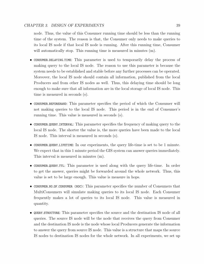
node in the ring. As in Figure 3.2 (a), backbone nodes are nodes 1, 2 and 3. Leaf-node is
the node that connects to backbone node. For instance, Figure 3.2 (a) shows that nodes 4,
5 and 6 are leaf-nodes of nodes 1, 2 and 3, respectively.
In order to find out the appropriate value for parameter NOP, we introduce two concepts
WORKLOAD and CAPACITY. We assume that the resource information travels around
the whole network.
Before setting up the formula, several terms are introduced as follow:

CHAPTER 3. DESIGN OF EXPERIMENTS 41
• NON is the total number of running IS nodes in the system;
• NOP is the number of Producers running in the same machine with IS node, and
publishing information to IS node;
• NOL is the number of leaf-nodes that connect to 1 backbone node.
• WORKLOAD of an IS node is the number of sites of which resource information goes
through that IS node;
• CAPACITY is the largest workload that a node can support without any error.
For example, if we have a network of 1 node, and 10 Producers connect to this node, the
workload of this node is equal to the number of Producers. However, the situation becomes
more complicated when the network has more nodes and different structure. In almost all
of our experiments, we use symmetric network structure as the main network topology of
the system. Figure 3.2 (a), (b) and (c) show 3 samples of network with 6, 8, 15 node,
respectively. We will set up a formula to estimate the workload.
Figure 3.2 (a) shows a network with 6 nodes. NON is 6; NOP is set to 10; NOL is 1; We will
estimate the workload for node 1. Assume that the information travels around the whole
network, and thus the information that goes through node 1 is from two sides. First, resource
information goes from the node 4 (a leaf-node) through node 1 to all other nodes. Second,
resource information from the remaining nodes (1, 2, 3, 5 and 6) goes to node 4 through
node 1.
NOP is 10, which means that the MultiProducers will simulate 10 Producers publishing 10
site’s information to local IS node, and thus in the local IS node, there is 10 site’s information
stored. As a result, from node 4, 10 site’s information will go through node 1 in order to
travel around the whole network. Because there is only 1 leaf-node, the total number of
information from leaf-node goes through node 1 is:
NOL * NOP = 1 * 10 (3.1)
From the other side, there are 4 nodes (2, 3, 5 and 6), and thus the total information that
goes to node 4 is from local information of node 1 and all information of those 4 nodes:
1 * NOP + 4 * NOP = 1 * 10 + 4 * 10 (3.2)

CHAPTER 3. DESIGN OF EXPERIMENTS 42
As a result, the workload of node 1 is the sum of information that goes from both sides.
From formula 3.1 and 3.2 we have:
WORKLOAD = 1 * 10 + 1 * 10 + 4 * 10 = 1 * 6 * 10 (3.3)
Formula 3.3 is, in fact,
WORKLOAD = NOL * NON * NOP (3.4)
Reasoning in the same way for 2 network structures shown in Figure 3.2 (b) and (c), we also
have the formula 3.4. In short, for symmetric network structures the formula to estimate
the workload is formula 3.4.
Thus, if we know the capacity (the largest workload) of a node, the value of NOP can be
estimated by the following formula:
NOP =CAPACITYNON * NOL
(3.5)
To find out this capacity, we design a experiment with only 1 node (NON=1), and increase
the number of Producers (NOP) until this node can not process any published information
from local Producers. The design of this experiment is in Section 3.3 and the result is in
Section 4.1.
Although the values of workload and capacity are not completely precise, using this value
helps setting up of all experimental environments with reasonable NOP values.
3.2.5 Time To Live (TTL)
There are 2 types of TTL, 1 for information traveling (PRODUCER STATIC TTL and
PRODUCER DYNAMIC TTL) and 1 for query forwarding (CONSUMER QUERY TTL).
Choosing the value for them has the same manner. For information traveling, the value
of TTL specifies how many hops the information can travel (with the assumption that the
life-time of information is long enough). For query forwarding, the value of the TTL specifies
how many hops the query can be forwarded. As a consequence, the total time information
traveling will increase if the information travels more and more. Besides, the response time
also increases if queries have to forward to more hops.

CHAPTER 3. DESIGN OF EXPERIMENTS 43
For almost all of our experiments, the TTL is set to be large enough such that the information
can travel around the whole network, and the query can be forwarded to all the nodes to
get the expected answer.
For example, with the 6 nodes network shown in Figure 3.2 (a), from any node, the longest
number of hops is 3 (from node 6 to 4, 6 to 5, or 5 to 4). As a result, we choose the TTL to
be 4 (1 more hop).
Figure 3.2 (b) shows another example with 8 nodes network. From any node, the longest
number of hops is 4 (from node 6 - 2 - 1 - 4 - 8). As a result, we choose the TTL to be 5.
The reason of adding 1 more into TTL value is that, in experiments, sometime a node can
be busy. Another reason is that in our system, we transfer information from one node to
others periodically. Thus, in some cases, resource information has to wait for the periodic
interval in order to be transfered. One mechanism in our system is that information will not
be forwarded duplicately. As a consequence, information may go in other way that requires
1 more hop. We expect that, adding 1 more into TTL is enough for information to travel
around the whole network.
3.3 Capacity
In this section, we briefly describe the experimental configuration to evaluate the limit of a
single IS node. The goal of this experiment is to find the capacity of single IS node. Since
the resource information is periodically published by Producers into the IS node, we consider
the following:
• How many sites are provided by Producers to a single IS node within a specific period?
(Inserting and updating for both static and dynamic information)
• How long does it take to insert and/or update for static and dynamic information to
a single IS node with query answering?
By evaluating these questions, we can determine the limit number of sites for a single IS
node. In order to determine the workload of an IS node, we design an experiment as follows.
We set up the network with 7 brother machines in which there is one running both ISNode
and MultiConsumer. The MultiConsumer simulates a predefined number of Consumers
querying the IS node for 1.5 minute. Each Consumer creates and sends a query to the IS
node every second. The query is for the whole resource information of a randomly chosen

CHAPTER 3. DESIGN OF EXPERIMENTS 44
site. 6 other machines will be running 6 MultiProducers, and totally 7 machines at benedict
cluster are involved. The MultiProducer simulates predefined number of Producers (NOP)
publishing information to local IS node. The results are recorded in log files during the
running time of the system. We set the system running time about 2 minutes. Other
parameters are also defined in table 3.2.
Parameters for ISNode
ISNODE RUNNING TIME = 2m
Parameters for Producer
PRODUCER RUNNING TIME = 1m30s
PRODUCER STATIC PUBLISH INTERVAL = 30s
PRODUCER DYNAMIC PUBLISH INTERVAL = 15s
PRODUCER DELAYING TIME = 10s
PRODUCER STATIC TTL = 0
PRODUCER DYNAMIC TTL = 0
PRODUCER NO OF INSTANCE = 400
Parameters for Consumer
CONSUMER RUNNING TIME = 1m30s
CONSUMER NO OF CONSUMER = 100
CONSUMER QUERY TTL = 5
CONSUMER QUERY INTERVAL = 6
CONSUMER DELAYING TIME = 24s
CONSUMER BEFOREHAND = 15s
CONSUMER QUERY LIFETIME = 1m
Table 3.2: Parameters - IS node capacity
The predefined number of Consumers (NOC) is 100 and does not change during the experi-
ment. The goal of this experiment is to determine a reasonable total number of Producers
that a single IS node can support.
We set the static and dynamic TTL=0 to guarantee that the resource information only
comes from Producers to local IS node and no longer travels. The IS node has its own log
file that records the resource information provided by its Producers. We observe and record
the total number of Producers (TNOP) in an IS node’s data storage every second. The
intervals for publishing static and dynamic information of Producers are 30 and 15 seconds,
respectively. Thus, we expect that we can find out the maximum TNOP that a single IS
node can support by increasing the value of TNOP. More specifically, it takes a period of
time to insert or update the information of all sites, and that period is known as inserting
and/or updating duration. Therefore, the maximum TNOP will be determined when the
inserting or updating duration is close to the publishing interval and the Consumers can still
be served.

CHAPTER 3. DESIGN OF EXPERIMENTS 45
3.4 Availability
Availability is desirable for a good GIS. First of all, in order to find out how well a single IS
node serves Consumers, we design an experiment as shown in Figure 3.3. The parameters
are shown in Table 3.3.
Figure 3.3: 1 IS node with increasing number of Consumers
Parameters for ISNode
ISNODE RUNNING TIME = 3m
ISNODE STATIC PUBLISH INTERVAL = 30s
ISNODE DYNAMIC PUBLISH INTERVAL = 15s
Parameters for Producer
PRODUCER RUNNING TIME = 2m50s
PRODUCER STATIC PUBLISH INTERVAL = 30s
PRODUCER DYNAMIC PUBLISH INTERVAL = 15s
PRODUCER DELAYING TIME = 6s
PRODUCER STATIC TTL = 0
PRODUCER DYNAMIC TTL = 0
PRODUCER NO OF INSTANCE = 10
Parameters for Consumer
CONSUMER RUNNING TIME = 2m30s
CONSUMER NO OF CONSUMER = increasing
CONSUMER QUERY TTL = 5
CONSUMER QUERY INTERVAL = 1s
CONSUMER DELAYING TIME = 30s
CONSUMER BEFOREHAND = 30s
CONSUMER QUERY LIFETIME = 1m
Table 3.3: Parameters – 1 IS node with increasing number of Consumers
Three brother machines run ISNode, MultiConsumer and MultiProducer respectively. The
system running time is 3 minutes. The MultiProducer simulates 10 Producers publishing
resource information to the IS node, which means resource information of 10 sites is in the
local storage of the IS node. The MultiConsumer simulates a predefined number of Con-
sumers querying the IS node for 1.5 minute. Each Consumer creates and sends a query to the
IS node every second. The only query created is the one for the whole resource information

CHAPTER 3. DESIGN OF EXPERIMENTS 46
of a randomly chosen site, and the life-time of a query is 1 minute. The predefined numbers
of Consumers are 100, 200, 300, ...
We expect that one IS node can support queries from a large number of Consumers, and
the performance is acceptable. We guess when the number of Consumers is increasing, the
throughput of query answering will increase but the response time will also increase. We
expect to find out the maximum number of Consumers one IS node can serve.
3.5 Scalability
In order to verify how well our GIS system can scale when increasing the number of running IS
nodes, we design a series of experiments with different network size. Each ISNode in our GIS
system will run at 1 brother machine. In addition, the MultiConsumer and MultiProducer
will also be run at the same machine where ISNode runs. Thus, the ISNode will be considered
as local ISNode to MultiProducer and MultiConsumer, respectively.
For the first 3 network sizes (6, 8 and 15 nodes), we run experiments with a large enough
TTL such that all the information can travel around the whole network.
For the 24 and 36 nodes network respectively, the TTL is varied in order to observe different
behaviors of the system when the information does not travel (TTL=0), travels 1 hop away
(TTL=1), and travels around the whole network when the TTL is large enough. The results
of those experiments can show the best TTL parameters for our system to run effectively.
The total number of consumers (TNOC)1 is also varying in each network size to see how
good our system can be.
The total number of Producers (TNOP) is fixed for our experiments. The value for NOP
is chosen as described in Section 4.1.1. The purpose of fixing TNOP is that we want verify
our GIS system behavior when varying the network size and the TNOC.
There are 5 focuses in doing each experiment. Section 3.5.1 describes the focuses related
to query answering, and the remaining focuses are for information traveling as described in
Section 3.5.2.
As described in Section 2.3.4, there are 3 query types. However, in all of our experiments,
we only use one query type for simplicity. This query type is the one that gets the whole
cluster information.
1TNOC is the sum of all Consumers making queries to our GIS system.

CHAPTER 3. DESIGN OF EXPERIMENTS 47
3.5.1 Query answering performance
For query answering, we focus on 3 important things as follows:
1. Determine the TNOC that our system can support by checking the data whenever
some abnormal behaviors occur.
2. Determine how quickly the system can answer all the queries by using the average
response time, regarding the TNOC in the system.
3. Determine the total throughput (queries/second) in the system when the TNOC is
increasing. The total throughput is the sum of all queries that the system can be
answered in 1 second.
With each experiment, we expect the system runs correctly and want to find out the result
for our focuses before the IS node reaches its limitation. The limitation is the point that our
system behaves abnormal when increasing the TNOC, for example, a lot of queries can not
be answered or the response time is very long.
1. For the first focus, we want to find the maximum TNOC by observing number of
queries that have been made and number of queries that have been answered. The
graph should show an gradually increasing line when increasing the TNOC until the
maximum TNOC that the system can support.
2. For the second focus, the average response time vs Consumers, we expect that the
average response time is not very long. When the TNOC increases, the response time
should only increase gradually.
3. We also expect that the throughput is also increasing when the TNOC increases and
the trend is also linear.
3.5.2 Information traveling performance
For the information traveling, we consider some issues as follows:
• How long does the resource information at Producers take to travel on the whole
network.
• The traveling time will not be longer than the life-time of information.

CHAPTER 3. DESIGN OF EXPERIMENTS 48
In our implementation, since the simulated resource information is published from Producers,
the traveling time of resource information is actually the duration in which there are two
phases:
• Publishing time: This is the period when resource information is published by Pro-
ducers to local IS node.
• Traveling time: This is the period when the resource information travels among IS
nodes.
During all experiments, we would like to see how quickly the information (static and dy-
namic) can be published from Producers to their local IS node (0 hop away), and travel
around the whole network regarding the number of hops (1, 2, 3, etc hop away). More
specifically, the more hops the resource information travels, the longer average information
traveling time is. We guess the average traveling time is going to increase regarding the
number of hops, and the trends should be linear.
In addition, we also expect that the maximum average traveling time to the farthest hop
should be smaller than the life-time of information. Although this parameter is defined as
10 minutes throughout our experiments in order to see the system’s behavior, it could be
5 and 1 minute for static and dynamic information, respectively in reality. We want to see
the traveling time in all experiment should not be larger than 5 and 1 minute for static and
dynamic information, respectively.
By having the timestamps when the resource information travel, we can measure the duration
of the information traveling in our experiments. The data collected in all experiments will
be represented by using graph.
3.5.3 Experiment with 6 nodes
In this experiment, we set up a symmetric network structure of 6 nodes (see Figure 3.4)
with 3 backbone nodes. Table 3.4 shows the configuration for this experiment. The system
running time is 10 minutes. The delaying time for starting publish information from local
Producers is 10 seconds. The TTL is set to 4, so that all information can travel around the
whole network. The total number of Producers (TNOP) will be set when we have the result
of capacity that a node can support.
The NOC value, namely the number of Consumers that the MultiConsumer is simulating,
is varied from 30, 60, 90, and so on. The MultiProducer simulates number of Producers (X
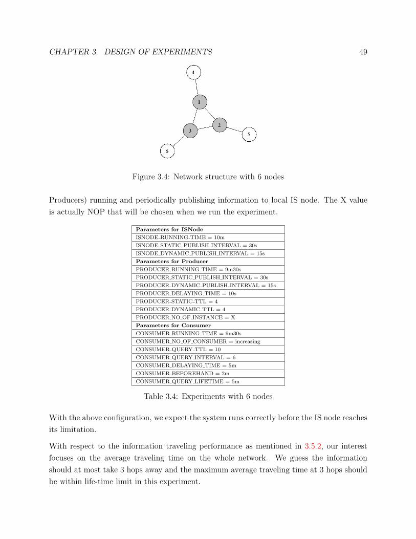
CHAPTER 3. DESIGN OF EXPERIMENTS 49
Figure 3.4: Network structure with 6 nodes
Producers) running and periodically publishing information to local IS node. The X value
is actually NOP that will be chosen when we run the experiment.
Parameters for ISNode
ISNODE RUNNING TIME = 10m
ISNODE STATIC PUBLISH INTERVAL = 30s
ISNODE DYNAMIC PUBLISH INTERVAL = 15s
Parameters for Producer
PRODUCER RUNNING TIME = 9m30s
PRODUCER STATIC PUBLISH INTERVAL = 30s
PRODUCER DYNAMIC PUBLISH INTERVAL = 15s
PRODUCER DELAYING TIME = 10s
PRODUCER STATIC TTL = 4
PRODUCER DYNAMIC TTL = 4
PRODUCER NO OF INSTANCE = X
Parameters for Consumer
CONSUMER RUNNING TIME = 9m30s
CONSUMER NO OF CONSUMER = increasing
CONSUMER QUERY TTL = 10
CONSUMER QUERY INTERVAL = 6
CONSUMER DELAYING TIME = 5m
CONSUMER BEFOREHAND = 2m
CONSUMER QUERY LIFETIME = 5m
Table 3.4: Experiments with 6 nodes
With the above configuration, we expect the system runs correctly before the IS node reaches
its limitation.
With respect to the information traveling performance as mentioned in 3.5.2, our interest
focuses on the average traveling time on the whole network. We guess the information
should at most take 3 hops away and the maximum average traveling time at 3 hops should
be within life-time limit in this experiment.

CHAPTER 3. DESIGN OF EXPERIMENTS 50
3.5.4 Experiment with 8 nodes
This experiment is almost the same as before (see Section 3.5.3), except that we change the
number of nodes (8 nodes) and the network shape (see Figure 3.5). In this experiment, we
use 4 backbone nodes, while in 6 nodes network, it is 3. Table 3.5 shows the configuration for
this experiment. Almost all of parameters are similar to the experiment of 6 nodes network.
The NOP for each IS node will be chosen when experiments are executed.
Figure 3.5: Network structure with 8 nodes
Parameters for ISNode
ISNODE RUNNING TIME = 10m
ISNODE STATIC PUBLISH INTERVAL = 30s
ISNODE DYNAMIC PUBLISH INTERVAL = 15s
Parameters for Producer
PRODUCER RUNNING TIME = 9m30s
PRODUCER STATIC PUBLISH INTERVAL = 30s
PRODUCER DYNAMIC PUBLISH INTERVAL = 15s
PRODUCER DELAYING TIME = 10s
PRODUCER STATIC TTL = 5
PRODUCER DYNAMIC TTL = 5
PRODUCER NO OF INSTANCE = X
Parameters for Consumer
CONSUMER RUNNING TIME = 9m30s
CONSUMER NO OF CONSUMER = increasing
CONSUMER QUERY TTL = 10
CONSUMER QUERY INTERVAL = 6
CONSUMER DELAYING TIME = 5m
CONSUMER BEFOREHAND = 2m
CONSUMER QUERY LIFETIME = 5m
Table 3.5: Experiments with 8 nodes
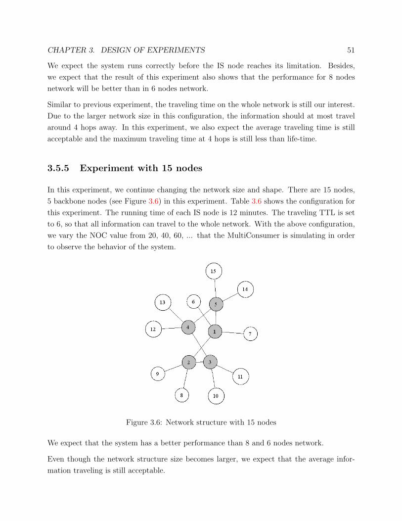
CHAPTER 3. DESIGN OF EXPERIMENTS 51
We expect the system runs correctly before the IS node reaches its limitation. Besides,
we expect that the result of this experiment also shows that the performance for 8 nodes
network will be better than in 6 nodes network.
Similar to previous experiment, the traveling time on the whole network is still our interest.
Due to the larger network size in this configuration, the information should at most travel
around 4 hops away. In this experiment, we also expect the average traveling time is still
acceptable and the maximum traveling time at 4 hops is still less than life-time.
3.5.5 Experiment with 15 nodes
In this experiment, we continue changing the network size and shape. There are 15 nodes,
5 backbone nodes (see Figure 3.6) in this experiment. Table 3.6 shows the configuration for
this experiment. The running time of each IS node is 12 minutes. The traveling TTL is set
to 6, so that all information can travel to the whole network. With the above configuration,
we vary the NOC value from 20, 40, 60, ... that the MultiConsumer is simulating in order
to observe the behavior of the system.
Figure 3.6: Network structure with 15 nodes
We expect that the system has a better performance than 8 and 6 nodes network.
Even though the network structure size becomes larger, we expect that the average infor-
mation traveling is still acceptable.
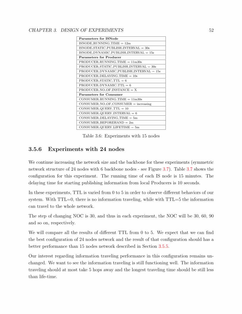
CHAPTER 3. DESIGN OF EXPERIMENTS 52
Parameters for ISNode
ISNODE RUNNING TIME = 12m
ISNODE STATIC PUBLISH INTERVAL = 30s
ISNODE DYNAMIC PUBLISH INTERVAL = 15s
Parameters for Producer
PRODUCER RUNNING TIME = 11m30s
PRODUCER STATIC PUBLISH INTERVAL = 30s
PRODUCER DYNAMIC PUBLISH INTERVAL = 15s
PRODUCER DELAYING TIME = 10s
PRODUCER STATIC TTL = 6
PRODUCER DYNAMIC TTL = 6
PRODUCER NO OF INSTANCE = X
Parameters for Consumer
CONSUMER RUNNING TIME = 11m30s
CONSUMER NO OF CONSUMER = increasing
CONSUMER QUERY TTL = 10
CONSUMER QUERY INTERVAL = 6
CONSUMER DELAYING TIME = 5m
CONSUMER BEFOREHAND = 2m
CONSUMER QUERY LIFETIME = 5m
Table 3.6: Experiments with 15 nodes
3.5.6 Experiments with 24 nodes
We continue increasing the network size and the backbone for these experiments (symmetric
network structure of 24 nodes with 6 backbone nodes - see Figure 3.7). Table 3.7 shows the
configuration for this experiment. The running time of each IS node is 15 minutes. The
delaying time for starting publishing information from local Producers is 10 seconds.
In these experiments, TTL is varied from 0 to 5 in order to observe different behaviors of our
system. With TTL=0, there is no information traveling, while with TTL=5 the information
can travel to the whole network.
The step of changing NOC is 30, and thus in each experiment, the NOC will be 30, 60, 90
and so on, respectively.
We will compare all the results of different TTL from 0 to 5. We expect that we can find
the best configuration of 24 nodes network and the result of that configuration should has a
better performance than 15 nodes network described in Section 3.5.5.
Our interest regarding information traveling performance in this configuration remains un-
changed. We want to see the information traveling is still functioning well. The information
traveling should at most take 5 hops away and the longest traveling time should be still less
than life-time.
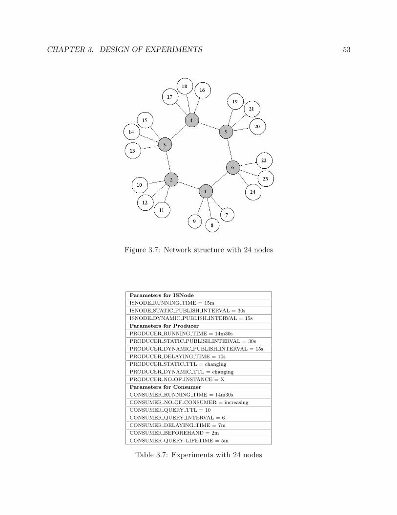
CHAPTER 3. DESIGN OF EXPERIMENTS 53
Figure 3.7: Network structure with 24 nodes
Parameters for ISNode
ISNODE RUNNING TIME = 15m
ISNODE STATIC PUBLISH INTERVAL = 30s
ISNODE DYNAMIC PUBLISH INTERVAL = 15s
Parameters for Producer
PRODUCER RUNNING TIME = 14m30s
PRODUCER STATIC PUBLISH INTERVAL = 30s
PRODUCER DYNAMIC PUBLISH INTERVAL = 15s
PRODUCER DELAYING TIME = 10s
PRODUCER STATIC TTL = changing
PRODUCER DYNAMIC TTL = changing
PRODUCER NO OF INSTANCE = X
Parameters for Consumer
CONSUMER RUNNING TIME = 14m30s
CONSUMER NO OF CONSUMER = increasing
CONSUMER QUERY TTL = 10
CONSUMER QUERY INTERVAL = 6
CONSUMER DELAYING TIME = 7m
CONSUMER BEFOREHAND = 2m
CONSUMER QUERY LIFETIME = 5m
Table 3.7: Experiments with 24 nodes

CHAPTER 3. DESIGN OF EXPERIMENTS 54
3.5.7 Experiments with 36 nodes
This is the largest network size in our experiments. Figure 3.8 shows a symmetric network
of 36 nodes with 6 backbone nodes. Table 3.8 shows the configuration for this experiment.
The running time of each IS node is 16 minutes.
In these experiments, the TTL is varied from 4 to 6 in order to verify different behaviors of
our system.
Figure 3.8: Network structure with 36 nodes
The MultiConsumer simulates an increasing NOC value is 30, 60, 90, ... for each experiment.
With this largest network size in our experiments, we expect the system will has the best
performance.
For information traveling performance, we still expect that the information traveling is still
working well.
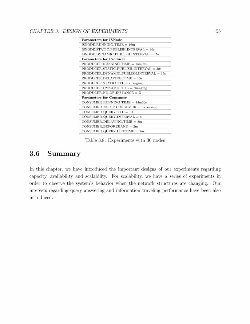
CHAPTER 3. DESIGN OF EXPERIMENTS 55
Parameters for ISNode
ISNODE RUNNING TIME = 16m
ISNODE STATIC PUBLISH INTERVAL = 30s
ISNODE DYNAMIC PUBLISH INTERVAL = 15s
Parameters for Producer
PRODUCER RUNNING TIME = 15m30s
PRODUCER STATIC PUBLISH INTERVAL = 30s
PRODUCER DYNAMIC PUBLISH INTERVAL = 15s
PRODUCER DELAYING TIME = 10s
PRODUCER STATIC TTL = changing
PRODUCER DYNAMIC TTL = changing
PRODUCER NO OF INSTANCE = X
Parameters for Consumer
CONSUMER RUNNING TIME = 14m30s
CONSUMER NO OF CONSUMER = increasing
CONSUMER QUERY TTL = 10
CONSUMER QUERY INTERVAL = 6
CONSUMER DELAYING TIME = 8m
CONSUMER BEFOREHAND = 2m
CONSUMER QUERY LIFETIME = 5m
Table 3.8: Experiments with 36 nodes
3.6 Summary
In this chapter, we have introduced the important designs of our experiments regarding
capacity, availability and scalability. For scalability, we have a series of experiments in
order to observe the system’s behavior when the network structures are changing. Our
interests regarding query answering and information traveling performance have been also
introduced.

Chapter 4
Results
In this chapter, we will describe all experimental results that we got.
In Section 4.1, we will describe the first series of experiments regrading the capacity of our
system. The results can help choosing a reasonable value for TNOP for each experiment
that will be carried out later.
The second series of experiments will describe the extreme case as can be seen in Section
4.2. The results can answer the question how many Consumers that our system of 1 node
can support.
The last series of experiments focus on scalability (see Section 4.3). Several network sizes
will be examined. The TNOC will also be varied while the TNOP is fixed.
4.1 Capacity
We have described the experiment in section 3.3. This section is dedicated to explanation
after the collection of data during experiment.
We started the experiment by increasing TNOP from 300, 400, etc distributed on 6 machines
running MultiProducers. We observed and examined the change in the number of sites
of single IS node within every second. When the TNOP was less than 2400, three our
components worked well. But with an increase in TNOP up to 2400, we got valuable results
as described below.
Figure 4.1 (a) shows the number of sites (inserting and updating static information) is
linearly increasing when the time elapses. Similarly, the results for dynamic information are
56

CHAPTER 4. RESULTS 57
shown in figure 4.1 (b). For dynamic information, it takes about 15 seconds (for inserting)
and 8 seconds (updating) total 2400 sites into the IS node, whereas for static information, it
correspondingly takes 15 and 6 seconds to insert and update total 2400 sites into the IS node.
We believe this is the limit TNOP because the intervals for publishing dynamic and static
information are defined as 15 and 30 seconds, and the duration of inserting and updating
information (both static and dynamic information) into the IS node should not be larger
than these corresponding intervals.
(a) Static Information (b) Dynamic Information
Figure 4.1: Publishing information - With query answering
This experiment shows that a single IS node can support relatively large number of sites as
expected and 2400 can be roughly seen as the limit.
4.1.1 Capacity for all experiments
From Section 4.1, we found that 2400 is the maximum number of Producers that a node can
support. However, a question is how to choose the reasonable total number of Producers
(TNOP) for our experiments?
We will run a series of experiments regarding the scalability to see the system behavior and
performance. The largest network size in our experiment will be the network with 36 nodes.
We will use this size to estimate the TNOP of our system. We assume that the information
can travel around the whole network.
Using the formula 3.5, with WORKLOAD=2400, NON=36 and NOL=5, we have:

CHAPTER 4. RESULTS 58
NOP =2400
36 * 5= 13.33 (4.1)
For simplicity, we manually choose NOP = 10. Thus, the total NOP (TNOP) that our system
can support is TNOP = 10 * 36 = 360. In order to compare the results of different network
size, we keep this TNOP=360 for all configurations in our experiments regarding scalability.
As a result, the NOP that each IS node can support will depend on the number of nodes in
the network.
Formula 4.2 shows how to estimate the NOP for all of our network structure.
NOP =360
NON(4.2)
4.2 Availability
The setup of this experiment was described in Section 3.4. After successfully running the
experiment, we obtained some valuable results as described below.
Figure 4.2 (a) shows the number of queries made and answered while the number of Con-
sumers (NOC) is increasing. While NOC is equal to or less than 700, all the queries made
are answered. When NOC is 712, only 5 percent of queries made are answered, and the
CPU usage on the machine running ISNode and the machine running MultiConsumer is
very close to 100 percent. In addition, timeout errors occur at MultiConsumer, which means
the MultiConsumer cannot get any response from the ISNode in time. Thus, we believe at
this experiment the maximum number of Consumers that one IS node can serve is about
700.
Figure 4.3 (a) shows the average response time of query answering while NOC is increasing.
While NOC is equal to or less than 700, the average response time is no longer than 1.16
second. When NOC is 712, the average response time suddenly reaches 10.12 seconds.
Figure 4.3 (b) shows the average, minimum and maximum response time of query answering
while NOC is equal to or less than 700. The longest response time is 5.62 seconds while
NOC is 700.
Figure 4.2 (b) shows the throughput of query answering while NOC is increasing. The
maximum throughput is 115 queries per second, when NOC is 700. The throughput suddenly
falls down to 6 queries per second when NOC is 712.

CHAPTER 4. RESULTS 59
(a) (b)
Figure 4.2: Queries and Throughput vs Consumers
(c) (d)
Figure 4.3: Response time vs Consumers
CHAPTER 4. RESULTS 60
The results described above show that one IS node can serve a large number of Consumers,
namely 700, as we expected. The longest response time of query answering is 5.62 seconds
and the maximum throughput is 115 queries per second, so the performance is definitely
acceptable. Due to the high CPU usage, the GIS system stops working effectively while
NOC is larger than 700, so 700 can be considered as the maximum of Consumers that one
IS node can serve.
4.3 Scalability
In this section, we will describe the result of our experiments. With the information traveling
mechanism, the information can travel around the whole network, which means all nodes in
the network will have information of all sites. As a result, when a Consumer makes queries
to its local node, the information is at the local storage of local node. Thus the response
time is very quick.
4.3.1 Experiment with 6 nodes
The configuration of this experiment was described in Section 3.5.3. Applying the formula
4.2 to estimate the NOP, we have:
NOP = 3606 = 60
thus, in this experiment, the parameter NOP is set to be 60.
4.3.1.1 Query answering performance
In Figure 4.4 (a), the number of queries (NOQ) that have been made is equal to the NOQ
that have been answered when the total number of Consumers (TNOC) increases from 180
to about 2520. After the point that TNOC is 2520, the NOQ that have been answered goes
down sharply. With 2520 Consumers, our system can still answer 63000 queries correctly
with the average response time only about 1.14 seconds. Figure 4.4 (a) shows that the total
throughput is also increasing gradually and it peaks up at around 235 queries/second when
the TNOC is 2520. However, when the TNOC is larger than 2520, around 15 percent of
queries can not be answered and the throughput is going down.
Figure 4.5 (a) and (b) show the changing of response time when the TNOC increases; Figure
4.5 (a) in fact is the average line in Figure 4.5 (b). In Figure 4.5 (a), before the TNOC is larger

CHAPTER 4. RESULTS 61
(a) (b)
Figure 4.4: Queries and Throughput vs Consumers with 6 nodes
(a) (b)
Figure 4.5: Average and Max, Min, Average response time vs Consumers with 6 nodes

CHAPTER 4. RESULTS 62
than 2520, the average response time is not changing so much, just increasing slightly from 0
to 1 second. However, after the TNOC increases larger than 2520, the average response time
is changing rapidly to 2 seconds. Figure 4.5 (b) shows the relationship among the minimum,
average and maximum response time when the TNOC increases. The graph shows that the
minimum, average and maximum response time are increasing when the TNOC increases.
While the maximum of response time is around 11 seconds, the minimum is only 0.01 second.
The total maximum response time line in Figure 4.5 (b) shows an fluctuated increase, but
even at the peak of 2520 Consumers, the maximum response time is still acceptable (about
less than 12 seconds).
All things considered, the system works as expected with the TNOC less than or equal to
2520. We roughly conclude that for this network structure, 2520 Consumers is the limitation,
235 queries/second is the maximum throughput and 1.14s is the average response time.
4.3.1.2 Information traveling performance
(a) Static information (b) Dynamic information
Figure 4.6: Average traveling time vs Number of hops
Figure 4.6 (a) and (b) show the trend of traveling time vs the number of hops for static and
dynamic information, respectively. Actually, we have done this experiment on 14 samples
regarding the increasing TNOC on the whole network. The TNOC is increased from 180 to
2520. The results from this case are shown below. Each curve represents the traveling time
of each sample with the corresponding TNOC.

CHAPTER 4. RESULTS 63
(a) Static information (b) Dynamic information
Figure 4.7: Max, Min, Average traveling time vs Number of hops at limit point
Figure 4.6 (a) and (b) indicate that the trend of traveling time is linearly increasing regarding
the number of hops. Moreover, the maximum average traveling time for dynamic and static
information are about 36 and 80 seconds, respectively. The information traveling time is
within life-time limit.
As mentioned Section 4.3.1, 2520 NOC is the limit of this network structure. At this point,
the results shown in figure 4.7 (a) and figure 4.7 (b) also indicate that the maximum, mini-
mum and average duration of the information traveling are reasonable. For dynamic infor-
mation, the maximum, minimum and average traveling time at the last hop (hop=3) are
approximately 38, 21, and 27 seconds respectively, whereas for static information, these val-
ues are about 81, 80 and 80 seconds, respectively. However, static information takes 4 hops
way.
In this experiment, we set the TTL=4 in order to make the information travel around the
whole network. We guessed the maximum hop which the information could take is 3 hops
traveling. Nevertheless, from Figures 4.7 (a) to (b), we can see that the information traveling
takes 4 hops.
Figure 4.8 shows how information from node 4 travels 4 hops and arrives at node 5. This
happens due to the fact that information traveling is based on periodical actions happening
at IS nodes. At each publishing interval, information is transferred. If a piece of information
is so ’lucky’ that it arrives at a node right before the interval, it will quickly be transferred.
If it is so ’unlucky’ that it arrives right after the interval, it will have to wait for the next

CHAPTER 4. RESULTS 64
Figure 4.8: Network structure with 6 nodes
interval. As a result, information traveling through 1-3-2-5 arrives earlier and the same
information traveling through 1-2-5 will be discarded.
4.3.2 Experiment with 8 nodes
The configuration of this experiment was described in Section 3.5.4. Applying the formula
4.2 for estimating the NOP, we have:
NOP = 3608 = 45
thus, in this experiment, the parameter NOP is set to be 45. With the result of experiment
with 6 nodes, we realized that the maximum number of hops that information can travel is
even 4. It means that the information can travel 1 hop longer than the maximum number of
hops that we observe from the network structure. Thus, we wonder whether the information
can travel 2 hops longer than what we can observe. As a result, in this experiment, we set
the TTL to be 6 (2 hops longer).
4.3.2.1 Query answering performance
Overall, Figures 4.9 (a) and (b) and Figures 4.10 (a) and (b) show the same trend with
those graphs of the experiment with 6 nodes. The results show that in 8 nodes network, the
performance is better.
First, the total NOC (TNOC) that this 8 nodes network can support (about 2880 Consumers)

CHAPTER 4. RESULTS 65
(a) (b)
Figure 4.9: Queries and Throughput vs Consumers with 8 nodes
is larger than in 6 nodes (about 2520 Consumers).
(a) (b)
Figure 4.10: Average and Max, Min, Average response time vs Consumers with 8 nodes
Second, Figure 4.10 (a) shows that the average response time of 8 nodes with TNOC equal
to 2880 is only around 1.00 second, while in 6 nodes network, with a smaller TNOC (2520
Consumers) the average response time is about 1.14 seconds (Figure 4.5 (a)). It means, in
8 nodes network with 4 backbone nodes, queries can be answered faster than in 6 nodes
network with 3 backbone nodes.
Last, Figure 4.9 (b) shows that the throughput of 8 nodes network is also larger (269
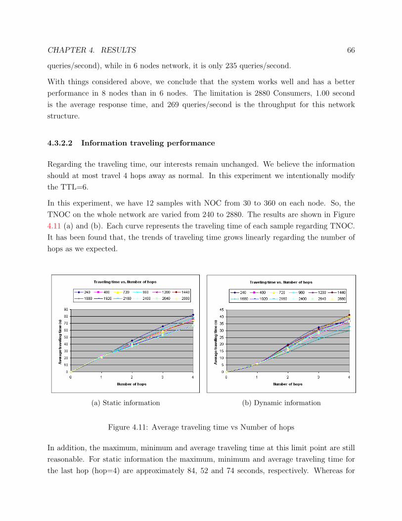
CHAPTER 4. RESULTS 66
queries/second), while in 6 nodes network, it is only 235 queries/second.
With things considered above, we conclude that the system works well and has a better
performance in 8 nodes than in 6 nodes. The limitation is 2880 Consumers, 1.00 second
is the average response time, and 269 queries/second is the throughput for this network
structure.
4.3.2.2 Information traveling performance
Regarding the traveling time, our interests remain unchanged. We believe the information
should at most travel 4 hops away as normal. In this experiment we intentionally modify
the TTL=6.
In this experiment, we have 12 samples with NOC from 30 to 360 on each node. So, the
TNOC on the whole network are varied from 240 to 2880. The results are shown in Figure
4.11 (a) and (b). Each curve represents the traveling time of each sample regarding TNOC.
It has been found that, the trends of traveling time grows linearly regarding the number of
hops as we expected.
(a) Static information (b) Dynamic information
Figure 4.11: Average traveling time vs Number of hops
In addition, the maximum, minimum and average traveling time at this limit point are still
reasonable. For static information the maximum, minimum and average traveling time for
the last hop (hop=4) are approximately 84, 52 and 74 seconds, respectively. Whereas for

CHAPTER 4. RESULTS 67
the dynamic information, these values are about 52, 22 and 36 seconds, respectively. The
information traveling has at most taken 4 hops even though the TTL is set to 6. This
indicates that the information traveling is functioning well as we expected.
The results are shown in Figure 4.12 (a) and (b). These values are also acceptable regarding
the life-time.
(a) Static information (b) Dynamic information
Figure 4.12: Max, Min, Average traveling time vs Number of hops at the limit point
4.3.3 Experiment with 15 nodes
The configuration of this experiment was described in Section 3.5.5. Applying the formula
4.2, we have:
NOP = 36015 = 24
thus, in this experiment, the parameter NOP is set to be 24. With the result of experiment
with 8 nodes, we realized that the maximum number of hops that information can travel is
only 4. Thus, for the following experiments, if we want the information can travel around
the whole network, the TTL will be 1 hop longer than what we can observe from the network
structure. As a result, in this experiment, we set the TTL to be 6 (1 more hop).

CHAPTER 4. RESULTS 68
(a) (b)
Figure 4.13: Queries and Throughput vs Consumers with 15 nodes
4.3.3.1 Query answering performance
Overall, Figures 4.13 (a), (b) and Figures 4.14 (a), (b) show the same trend with those
graphs of the experiments with 8 nodes. The results show that in 15 nodes network with 5
backbone nodes has a better performance.
First, from Figures 4.13 (a), the total NOC (TNOC) that this 15 nodes network (about 5700
Consumers) can support is approximately 2 times as in 8 nodes (about 2880 Consumers).
(a) (b)
Figure 4.14: Average and Max, Min, Average response time vs Consumers with 15 nodes
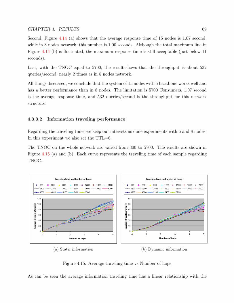
CHAPTER 4. RESULTS 69
Second, Figure 4.14 (a) shows that the average response time of 15 nodes is 1.07 second,
while in 8 nodes network, this number is 1.00 seconds. Although the total maximum line in
Figure 4.14 (b) is fluctuated, the maximum response time is still acceptable (just below 11
seconds).
Last, with the TNOC equal to 5700, the result shows that the throughput is about 532
queries/second, nearly 2 times as in 8 nodes network.
All things discussed, we conclude that the system of 15 nodes with 5 backbone works well and
has a better performance than in 8 nodes. The limitation is 5700 Consumers, 1.07 second
is the average response time, and 532 queries/second is the throughput for this network
structure.
4.3.3.2 Information traveling performance
Regarding the traveling time, we keep our interests as done experiments with 6 and 8 nodes.
In this experiment we also set the TTL=6.
The TNOC on the whole network are varied from 300 to 5700. The results are shown in
Figure 4.15 (a) and (b). Each curve represents the traveling time of each sample regarding
TNOC.
(a) Static information (b) Dynamic information
Figure 4.15: Average traveling time vs Number of hops
As can be seen the average information traveling time has a linear relationship with the

CHAPTER 4. RESULTS 70
number of hops as we expected. From those figures, the information traveling takes 5 hops.
The average traveling time for both dynamic and static information are still acceptable
regarding the life-time. More specifically, the maximum average traveling time for dynamic
and static information are about 50 and 110 seconds, respectively.
The limit TNOC of this network structure is 5700. For static information, at this point
the maximum duration of information traveling is about 85 seconds, whereas for dynamic
information, this value is 55 seconds. These results are shown in Figure 4.16 (a) and (b)
regarding static and dynamic information.
(a) Static information (b) Dynamic information
Figure 4.16: Max, Min, Average traveling time vs Number of hops at the limit point
4.3.4 Experiments with 24 nodes
The configuration of these experiments was described in Section 3.5.6. Applying the formula
4.2, we have:
NOP = 36024 = 15
thus, in this experiment, the parameter NOP is set to be 15.
Section 4.3.4.1 will compare the performance of 24 nodes network, 6 backbone nodes with
diferrent TTL values. Section 4.3.4.2 will describe the query answering performance of this
network structure with the best configuration and the last Section (Section 4.3.4.3) will show
the performance of of information traveling.

CHAPTER 4. RESULTS 71
4.3.4.1 Comparing performance with different TTL value
Figure 4.17 (a), (b) and (c) compare the performance of our system running with 24 nodes
and different TTL values (from 0 to 5). When the TTL is increasing, the maximum through-
put and the maximum TNOC that the system can support are also increased, but the average
response time is decreased. When the TTL is less than 4, the maximum throughput is slightly
changed with small values, from about 76 to 162 queries/second; the maximum TNOC is
also changing, from 720 to 1440 Consumers; and the average response time is between 3
and 4 seconds. However, when the TTL is 5, there is a sharply increase in both maximum
throughput and maximum TNOC, about 10 times in TNOC (8650 Consumers) more than
the first case when TTL is equal to 0 (720 Consumers), and 10 times in maximum through-
put (1032 queries/second) compared to the first case with only about 76 queries/seconds. In
Figure 4.17 (c), the result shows that the average response time reduces sharply from more
than 4 seconds to below 1 second.
(a) (b) (c)
Figure 4.17: Comparing performance with different TTL value of 24 nodes
From Figures 4.17 (a), (b) and (c), the results show that the performance is not good when
the TTL is small. It is worst when there is no information traveling at all (when TTL=0).
Thus, a question is why the performance is not good when the TTL is small? There are
several reasons for this issue, and we will describe as follow.
The first reason is because of the information traveling mechanism. If the TTL is small, re-
source information can not travel very far from the source node. As a result, when Consumer
makes queries that require information from very far nodes, queries have to be forwarded
several hops away in order to get answers. Consequently, the average response time should
be increased, and the maximum throughput and maximum TNOC, besides, are decreased.
If TTL is large enough, resource information can travel around the whole network, and as
a result, when Consumers make queries, IS nodes can answer immediately from the local

CHAPTER 4. RESULTS 72
storage. Thus, the performance will be much better.
The second reason is because of the query structure. As mentioned in Section 3.2.3, query
structure specifies the source and the destination IS node for all queries. In all of our
experiments, we varied the source and destination IS node, such that the distance between
2 node is various from 1 hop to 5 hops. As a result, if TTL is small, queries have to be
forwarded as most 5 hops in order to get the answer. Query forwarding very far will make
the performance worse.
In reality, if the network size is huge, resource information should not travel very far. Choos-
ing the best configuration for all network sizes is costly and nearly impossible, but for a
specific range of network size, at least we can find an reasonable configuration that has
acceptable performance.
4.3.4.2 Query answering performance
From the result shown in Section 4.3.4.1, we know that the network of 24 nodes has the best
answering performance when the TTL is 5. We will compare the result of this experiment
with the smaller network structure, namely 15 nodes network with 5 backbone nodes.
Overall, Figures 4.18 (a), (b) and Figures 4.19 (a) and (b) show the same trend with those
graphs of the experiments with 15 nodes. The results show that in 24 nodes network with
TTL equal to 5, the performance is better.
(a) (b)
Figure 4.18: Queries and Throughput vs Consumers with 24 nodes
First, the total NOC (TNOC) that this 24 nodes network can support is about 7920 Con-
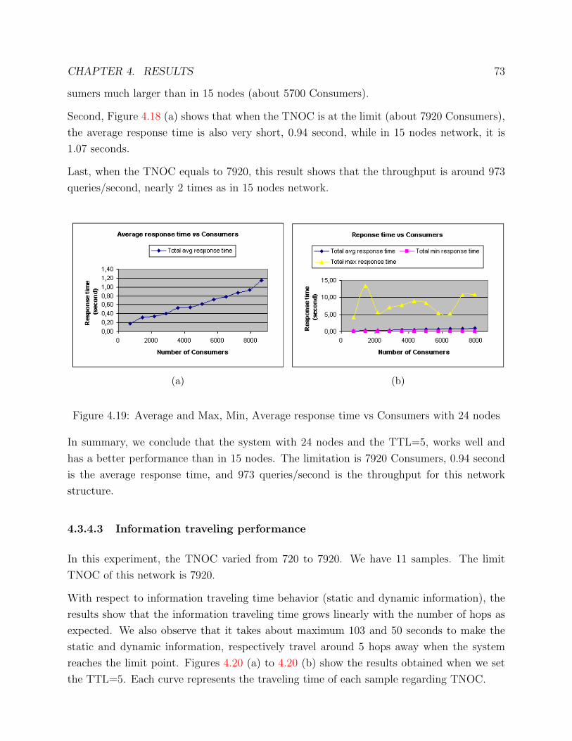
CHAPTER 4. RESULTS 73
sumers much larger than in 15 nodes (about 5700 Consumers).
Second, Figure 4.18 (a) shows that when the TNOC is at the limit (about 7920 Consumers),
the average response time is also very short, 0.94 second, while in 15 nodes network, it is
1.07 seconds.
Last, when the TNOC equals to 7920, this result shows that the throughput is around 973
queries/second, nearly 2 times as in 15 nodes network.
(a) (b)
Figure 4.19: Average and Max, Min, Average response time vs Consumers with 24 nodes
In summary, we conclude that the system with 24 nodes and the TTL=5, works well and
has a better performance than in 15 nodes. The limitation is 7920 Consumers, 0.94 second
is the average response time, and 973 queries/second is the throughput for this network
structure.
4.3.4.3 Information traveling performance
In this experiment, the TNOC varied from 720 to 7920. We have 11 samples. The limit
TNOC of this network is 7920.
With respect to information traveling time behavior (static and dynamic information), the
results show that the information traveling time grows linearly with the number of hops as
expected. We also observe that it takes about maximum 103 and 50 seconds to make the
static and dynamic information, respectively travel around 5 hops away when the system
reaches the limit point. Figures 4.20 (a) to 4.20 (b) show the results obtained when we set
the TTL=5. Each curve represents the traveling time of each sample regarding TNOC.

CHAPTER 4. RESULTS 74
(a) Static information (b) Dynamic information
Figure 4.20: Average traveling time vs Number of hops
In addition, for the limit point, the maximum traveling time for static information is about
116 seconds, whereas for dynamic information, this value is 59 seconds. These values are
still acceptable regarding the life-time. Figure 4.21 (a) and (b) show the results.
4.3.5 Experiments with 36 nodes
The configuration of these experiments was described in Section 3.5.7. Applying the formula
4.2, we have:
NOP = 36036 = 10
thus, in this experiment, the parameter NOP is set to be 10.
4.3.5.1 Comparing performance with different TTL value
Figure 4.22 (a) and (b) compare the performance of our system running with 36 nodes. The
TTL is varied from 4 to 6. When the TTL is increasing, the maximum throughput and the
maximum number of Consumers that the system can support are also increased. When the
TTL is 4 and 5, the graphs show that the maximum throughput does not change very much
(980 queries/second and 1003 queries/second for TTL=4 and TTL=5 respectively). The
maximum TNOC in both experiment is the same (8640 Consumers). However, when TTL

CHAPTER 4. RESULTS 75
(a) Static information (b) Dynamic information
Figure 4.21: Max, Min, Average traveling time vs Number of hops at the limit point
is set to 6, the performance is improved. The maximum throughput is about 200 more than
in the previous 2 experiments with smaller TTL. The maximum TNOC is also changed, up
to 10800. It means the system can support more Consumers (about 2000) than in previous
setup.
We have the same conclusion as in 24 nodes. It means when TTL is larger, the query
answering performance is better.
4.3.5.2 Query answering performance
We know that the network of 36 nodes has the best answering performance when the TTL
is 6. We will compare the result of this experiment with the smaller network structure.
Overall, the 4 graphs as in Figures 4.23 (a), (b) and Figures 4.24 (a) and (b) show the same
trend with those graphs of the experiments with 24 nodes. The results show that in 36 nodes
network, the performance is better.
First, the total NOC (TNOC) that this 36 nodes network is about 9720 Consumers much
larger than in 24 nodes (about 7920 Consumers).
Second, Figure 4.24 (a) shows that, the average response time of 36 nodes when the TNOC
peaks up at the limit (about 9720 Consumers) is 0.83 second, while in 24 nodes network,
this number is 0.94 seconds (Figure 4.24 (a)).

CHAPTER 4. RESULTS 76
(a) (b)
Figure 4.22: Maximum throughput and Consumers vs TTL of 36 nodes
(a) (b)
Figure 4.23: Queries and Throughput vs Consumers with 36 nodes

CHAPTER 4. RESULTS 77
(a) (b)
Figure 4.24: Average and Max, Min, Average response time vs Consumers with 24 nodes
The total throughput for 36 nodes network with 6 backbone has the throughput of 1128
queries/second, whereas in 24 nodes, this throughput is 973 queries/second.
All things considered, we conclude that the system of 36 nodes with TTL is 6 has a better
query answering performance than in 24 nodes network with the same backbone struc-
ture. The limitation is 9720 Consumers, 0.83 second is the average response time, and 1128
queries/second is the throughput for this network structure.
4.3.5.3 Information traveling performance
In this experiment, we have 9 samples with TTL=6 the TNOC varied from 1080 to 9720.
The limit TNOC of this network is 9720.
Figures 4.25 (a) to 4.25 (b) show the results obtained when we set the TTL is equal to 6.
Each curve represents the traveling time of each sample regarding TNOC.
With respect to information traveling time behavior (static and dynamic information), the
results show that the trend of information traveling time grows linearly as expected. We also
observe that it takes about maximum 112 and 52 seconds to make the static and dynamic
information, respectively travel around 6 hops away when the system reaches the limit point.
At the limit point, the maximum traveling time for static information is about 97 seconds,
whereas for dynamic information, this value is 46 seconds. The information traveling only
takes 5 hops, and these values are still acceptable regarding the life-time.

CHAPTER 4. RESULTS 78
(a) Static information (b) Dynamic information
Figure 4.25: Average traveling time vs Number of hops
(a) Static information (b) Dynamic information
Figure 4.26: Max, Min, Average traveling time vs Number of hops at the limit point

CHAPTER 4. RESULTS 79
All our concerns are examined regarding the information traveling performance during all
experiments. From the results, we realize that the average traveling time is reasonable and
acceptable with respect to the life-time even for the largest network structure that we have
done. As a consequence, we believe that the information traveling is functioning well.
4.4 Summary
We have described the results of our experiments. Regarding the scalability, although we
cannot conclude that our system is scalable, but at least, we are convinced that the system
appears to be scalable. The performance is quite good and the maximum TNOC and TNOP
that our system can support are also very large.

Chapter 5
Analysis
In this chapter, we analyze experimental results obtained before, and present some conclu-
sions regarding scalability and information traveling in Section 5.1 and 5.2 respectively. For
the purpose of observing the influence of network shape, we design some new experiments,
as described in Section 5.3.
5.1 Scalability
In all the experimental results regarding scalability described in Section 4.3, the data col-
lected at the specific moment when the total number of Consumers that can be served and
the total throughput arrive at the peak are most valuable. These data show that under a
fixed number of sites, when the GIS network size, namely the number of IS nodes, is increas-
ing, the maximum total number of Consumers that can be served and the maximum total
throughput are also increasing but the average query response time is decreasing. Figure 5.1
(a), (b) and (c) depict the increasing and decreasing are all linear. In addition, as shown
in Figure 5.2 (a) and (b), resource information is traveling effectively around the whole GIS
network: for the static information, the maximum traveling time is less than 97 seconds; for
the dynamic, the maximum is less than 52 seconds.
We conclude that our GIS appears to be scalable. Under a fixed number of sites, when
the number of IS nodes is increasing, the performance of our GIS is also increasing but will
finally arrive at the peak. However, due to the limitation of the experimental environment,
we could not find out the peak.
80

CHAPTER 5. ANALYSIS 81
(a) (b) (c)
Figure 5.1: Maximum throughput, NOC, and Average response time vs Number of nodes
(a) (b)
Figure 5.2: Average static and dynamic information traveling time vs Number of hops

CHAPTER 5. ANALYSIS 82
5.2 Information traveling
For the purpose of showing the behavior of information traveling, we defined the life-time
of static and dynamic information both equal to 10 minutes in all the experiments that we
have done. In reality, these two parameters should not be so long, which means a piece of
resource information stops traveling further when its life-time is over.
Because in our GIS implementation, information traveling is based on periodical actions
happening at IS nodes, traveling time is proportional to the number of hops. As shown in
Figure 5.2 (a) and (b), one hop takes nearly 20 seconds for static information and nearly
9 seconds for dynamic. In addition to TTL, the life-time determines how far a piece of
information can travel.
5.3 Design of more experiments
In all experiments we have done, we manually chose the network shapes. Then a question
is: are those network shapes the best for the performance? We decide to carry out more
experiments so that we can see how the network shape influences the performance.
5.3.1 Experiment of 24 nodes with net backbone
The configuration of this experiment is almost the same as before (see Section 3.5.6), except
that the network shape is changed as shown in Figure 5.3. While previously the 24-node
network had a 6-node ring backbone, the new backbone has three more cross links. TTL of
resource information is set to 5.
The purpose of this experiment is to see whether a net backbone is better than a ring.
We expect that compared with the experiment done before, it will take shorter time for
information from leaf nodes to travel around the whole network due to the fact that the
longest distance is one hop shorter. We guess the maximum throughput and maximum total
number of Consumers that can be served will not change a lot due to the fact that the
number of IS nodes is unchanged.

CHAPTER 5. ANALYSIS 83
Figure 5.3: Network structure of 24 nodes with net backbone
5.3.2 Experiment of 24 nodes with line backbone
In this experiment, again we only change the network shape, as shown in Figure 5.4. The
new backbone is a line. Correspondingly, TTL of resource information is set to 7.
The purpose of this experiment is to see whether a line backbone makes a lot of difference.
We guess the maximum throughput and maximum total number of Consumers that can be
served will not change a lot, either. However, much longer time is needed for information
from devious leaf nodes to travel around the whole network due to the fact that these nodes
are connected to the end of the line backbone.
Figure 5.4: Network structure of 24 nodes with line backbone

CHAPTER 5. ANALYSIS 84
5.3.3 Experiment of 36 nodes with 5-node backbone
In this experiment we keep almost the same configuration as defined in Section 3.5.7, but the
network shape is changed as shown in Figure 5.5. The new 36-node network has a 5-node
ring backbone. Thus, TTL of resource information is set to 5.
By doing this experiment, we want to see what will happen if backbone nodes are reduced
while leaf nodes are augmented. Because the backbone is one hop smaller, we expect that it
will take shorter time for information from leaf nodes to travel around the whole network.
We guess changing the backbone will not highly influence the performance.
Figure 5.5: Network structure of 36 nodes with 5-node backbone
5.4 Summary
By analyzing the experimental results, we concluded that our GIS appears to be scalable.
It was confirmed that both TTL and the life-time determine how far a piece of information
can travel. We designed a few new experiments in order to see how network shape influences
the performance. The results of these experiments will be described in Chapter 6.
Chapter 6
More experiments
In this series of experiments, we will compare the experimental results with different setups
by using some important values. The objects to be compared are:
• 24 nodes with 6 ring backbone nodes vs 24 nodes with 6 net backbone nodes;
• 24 nodes with 6 ring backbone nodes vs 24 nodes with 6 line backbone nodes;
• 36 nodes with 6 ring backbone nodes vs 36 nodes with 5 ring backbone nodes;
Firstly, we compare the number of queries has been made and answered in order to find out
the maximum TNOC that the system can support in each setup. This number shows the
availability of the system with different setups.
Secondly, we compare the maximum throughput that the system with each setup can sup-
port.
Thirdly, we consider the maximum of average response time for each setup. This result
shows how quick the system can be for each network structure.
Lastly, we consider the information traveling time for each setup.
6.1 Compare 24 nodes between ring and net backbone
The setup of this experiment was described in Section 5.3.1. Section 6.1.1 will compare the
performance of 24 nodes network with net backbone with the ring backbone as mentioned
in Section 4.3.4.2 and Section 6.1.2 will show the performance of information traveling.
85

CHAPTER 6. MORE EXPERIMENTS 86
6.1.1 Query answering performance
(a) (b) (c)
Figure 6.1: Compare 24 nodes, 6 ring vs 6 net backbone nodes
Overall, the query answering performance is nearly the same in both setups, which are 24
nodes with ring backbone and 24 nodes with net backbone.
Figure 6.1 (a) shows that the number of queries that can be answer is similar. The total
number of queries that can be answered is the same as queries made around 435600 queries.
The maximum TNOC that our system can support is also the same about 7920 Consumers.
In Figure 6.1 (b), the maximum throughput is about 973 queries/second in both setups.
Figure 6.1 (c) shows that the maximum of average response time has similar values around
1 second.
For all results shown above, we observe that the query answering performance is simi-
lar in both setups. The limitation is 7920 Consumers, the maximum throughput is 973
queries/second, and the average response time is about 1 second.
6.1.2 Information traveling performance
Figure 6.2 (a) and (b) show the average traveling time for static and dynamic information in
both setups (24 nodes with ring backbone and 24 nodes with net backbone). Due to the fact
that information traveling can take one hop less in the network with net backbone, regarding
information traveling ring backbone is not as good as net backbone but still acceptable.

CHAPTER 6. MORE EXPERIMENTS 87
(a) Static information (b) Dynamic information
Figure 6.2: 24 nodes-6 ring backbone vs 24 nodes-net backbone
6.2 Compare 24 nodes between ring and line backbone
The setup of this experiment was described in Section 5.3.2. Section 6.2.1 will compare the
performance of 24 nodes network, ring backbone with 24 nodes, line backbone, as described
in Section 4.3.4.2 and Section 6.2.2 will show the performance of information traveling.
6.2.1 Query answering performance
(a) (b) (c)
Figure 6.3: Compare 24 nodes - 6 ring vs 6 line backbone node
Overall, the performance of query answering for 24 nodes with line backbone is worse than
in 24 nodes with ring backbone network structure.
Figure 6.3 (a) shows that the number of queries that can be answered in ring backbone
is much larger than in line backbone. The total number of queries that can be answered

CHAPTER 6. MORE EXPERIMENTS 88
is 435600 queries, whereas in line backbone, this number is just 396000 queries. While in
line backbone the maximum TNOC is about 7200, the maximum TNOC is 7920 in ring
backbone, 720 Consumers larger than in line backbone network.
In Figure 6.3 (b), the maximum throughput of ring backbone is about 973 queries/second,
while in line backbone, it is only about 885 queries/second.
The last Figure 6.3 (c) shows that the maximum of average response time has similar values,
around 1 second.
All things considered, we realize that the query answering performance of ring backbone is
better than line backbone network.
6.2.2 Information traveling performance
As can be seen in Figure 6.4 (a) and (b), the traveling time in 24 nodes with line backbone
is longer than that for 24 nodes with 6 ring backbone because information traveling takes
2 hops more in line backbone configuration. For dynamic information, in line backbone
configuration, the average traveling time is more than 60 seconds when the information
travels on the whole network (hop=7). For static information, the traveling time is still
acceptable. It just takes around 120 seconds to make the information travel at most 7 hops
away. With respect to the life-time, the traveling time for dynamic is unacceptable because
the life-time could be defined as 1 minute in reality.
By comparing the information traveling, we realize that the 24 nodes with ring backbone is
better than 24 nodes with line backbone.
6.3 Compare 36 nodes between 6 and 5 nodes ring
backbone
The setup of this experiment was described in Section 5.3.3. Section 6.3.1 will compare the
performance of 36 nodes network with 5 backbone nodes with the performance of 36 nodes
network with 6 backbone nodes as mentioned in Section 4.3.5.2. Section 6.3.2 will show the
performance of information traveling.

CHAPTER 6. MORE EXPERIMENTS 89
Static information (a) Dynamic information (b)
Figure 6.4: 24 nodes-line backbone vs 24 nodes-6 ring backbone
(a) (b) (c)
Figure 6.5: Compare 36 nodes - 6 ring vs 5 ring backbone nodes

CHAPTER 6. MORE EXPERIMENTS 90
6.3.1 Query answering performance
Overall, the performance of query answering for 36 nodes with 6 backbone and 5 backbone
nodes are similar.
Figure 6.5 (a) shows that the total number of queries that can be answered in 5 backbone
nodes is 437400 queries, whereas in 6 backbone nodes, this number is 437130 queries. The
maximum TNOC is the same in both network, about 9720.
In Figure 6.5 (b), the maximum throughput is completely similar, about 1128 queries/second.
The last Figure 6.5 (c) shows that the maximum of average response time has similar values,
around 1 second.
All things considered, we realize that the network with 5 backbone and 6 backbone nodes
have the same performance. Thus, we conclude that the backbone size does not affect the
query answering performance.
6.3.2 Information traveling performance
Static information (a) Dynamic information (b)
Figure 6.6: 36 nodes 5-node ring backbone vs 36 nodes with 6-node ring backbone
The traveling time results of 36 nodes with 6 backbone nodes and 36 nodes with 5 backbone
nodes are presented in Figure 6.6 (a) and (b). Due to the fact that information traveling
can take one hop less in the network with 5 backbone nodes, 6-node backbone is worse than
5-node backbone regarding information traveling but still acceptable.

CHAPTER 6. MORE EXPERIMENTS 91
6.4 Analysis
In Section 6.2, the results show that the 24 nodes with line backbone is not suitable for our
system. The performance is slightly less than in the 24 nodes with ring backbone, but the
traveling time is unacceptable. The maximum number of hops is 7, and in order to make
information travel around the whole network, the traveling time of dynamic information is
more than 1 minute. Besides, the line structure is not robust as the ring and net backbone.
The net backbone (see Section 6.1), on the other hand, seems to be similar to the ring
backbone. The performance of query answering is not different, but the result of the net
backbone shows that the traveling time is slightly less. Regarding information traveling, net
backbone looks better. However, we are not sure what will happen if the backbone is fully
connected.
Regarding the experiments with 36 nodes, the results show that the query answering per-
formance of 5 nodes and 6 nodes ring backbone is almost the same. This means reducing
1 node in the ring backbone does not influence very much to query answering when the
network size is the same. Regarding information traveling, 5-node backbone looks better.
We conclude that if information traveling is working correctly and effectively, the perfor-
mance of query answering will depend on the network size, namely the number of IS nodes,
not the network shape. The reason is: due to the fact that the TNOP is unchanged, as long
as information is effectively traveling around the whole network, a larger network size can
serve more Consumers and has better performance. However, the performance of information
traveling depends on both the network size and shape.
6.5 Summary
In this chapter, we introduced the results of a few new experiments that have been done for
the purpose of indicating the influence of network shape, and presented some new findings
based on these results.
Chapter 7
Related work
In this chapter, we will make the comparison of our experimental results with MDS. Two
other projects will also be introduced with brief evaluation.
7.1 Compare with MDS
Since we obtained the valuable results from the experiments as done above, we are interested
in the quantitative study of the performance of the current GISs. This is useful and can help
us understand the performance limitations in our system compared with other GISs.
To date, there are not many studies that quantitatively evaluate the performance of the
current GISs. We found that there is a good study of the performance of GIS [18]. They
performed the experiments to test the scalability of the dominant GISs such as: Globus
Toolkit Monitoring and Discovery Service (MDS2), the European Data Grid Relational
Monitoring Architecture (R-GMA), and Hawkeye a part of Condor project. These results
are really meaningful to us, and we take the results of MDS into consideration due to the
fact that MDS presents better scalability than others.
Recall chapters 4, 5 and 6, it can be seen that our system seems to scale well regarding the
total number of Consumers (TNOC) as well as total number of Producers (TNOP). The
maximum TNOC throughout our experiments that the system can support is from 2520 (6
nodes) to 10800 (36 nodes), while TNOP is fixed and equal to 360. For MDS, the maximum
number of users is only up to 600, and the maximum number of information servers is only
less than 100. The counterparts of MDS regarding TNOC and TNOP are number of users
and information servers.
92

CHAPTER 7. RELATED WORK 93
With respect to the response time, our results presented are quite good. Even in the worst
case (6 nodes), the results show that the average response time is less than 1.5 seconds,
while the number of Consumers is 2520. This result is even better when the system with 36
nodes, the response time is less than 1 second. For MDS, the average response time is also
small (less than 2 seconds) even as the number of users increases (up to 600). However, the
TNOC in our experiments (equivalent to number of users) is much larger than MDS.
Due to the large TNOC, our results also show a higher throughput compared with MDS.
The maximum throughput in 6 nodes is 235 queries/second, whereas for MDS, the maximum
throughput is approximately 140 queries/second.
From the observations and numbers above, we are very much interested in a question why
we got such interesting results in comparison with MDS. Obviously, this is promising in
building a more scalable GIS. These results can be explained by major reasons:
1. Our GIS is distributed structure because it is based on peer-to-peer model, while MDS
is centralized one. Thus, our GIS can support a lot of Consumers and Producers by
distributing them on the whole network. The aggregate directory server in MDS can
be the bottleneck when a large growing number of users are making concurrent queries
to it and there is too much resource information contained.
2. An outstanding feature of our GIS is information traveling. Almost all queries can be
answered locally when this feature is functioning. In MDS usually the queries have to
go down from the top to bottom in aggregate directory, so the response time therefore
might be longer than ours.
Nevertheless, it is difficult to conclude that our system is more scalable or better than MDS
due to some different settings as follows:
1. Experimental setup: In their experiments, all machines’ configurations are worse than
ours. The best machine is only equipped with 1133 MHz Intel PIII CPU and 512 MB
RAM, while our machines are more powerful with 2.8GHz Pentium IV and each have
2GB RAM. In addition, they ran the experiments on both sites with the bandwidth
around 55 Mbits/sec, while ours is Gigabit Ethernet network and our experiments are
run on one site. This is a cause of higher query response time in MDS.
2. Resource information size: Our resource information of a site simulated is only 7800
Bytes, whereas for their experiments, the resource information is real data with the
variable size. Hence, this is also the reason for longer response time and less throughput
in MDS.

CHAPTER 7. RELATED WORK 94
In summary, our analysis above shows that our proposed idea of building a scalable GIS is
promising. In our future work, we plan to do more experiments to deeply study and keep
evaluating our system. Especially, a setup close to MDS will be performed in order to have
a more accurate comparison.
7.2 Other peer-to-peer approaches
In this section, we introduce two other approaches of building GIS with peer-to-peer tech-
nology and then present a brief evaluation on these approaches. These two research groups
proposed an peer-to-peer (P2P) model to setup the underlying network among Virtual Orga-
nizations (VOs). More precisely, the topology is the super-peer network architecture rather
than a pure P2P network.
7.2.1 A peer-to-peer information service for Grid
System overview Sample networks
Figure 7.1: An example of super-peer network: (a) without redundancy; (b) with redun-
dancy. Black nodes represent super-peer. White nodes represent the regular peers [13]
This project [13] proposed an approach to build GIS based on peer-to-peer model. Figure
7.1 shows that the system consists of two main components:
• Agent, which runs on the regular peer node, is responsible for publishing local infor-
mation to the super-peer;
• Aggregator, which runs on super-peer, is responsible for collecting data, replying to
queries, and forwarding queries to other super-peers. The Aggregator also has an index
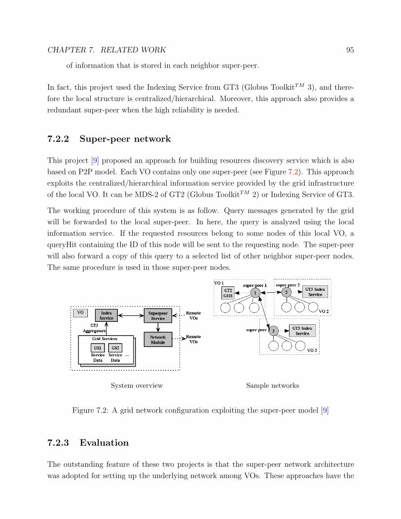
CHAPTER 7. RELATED WORK 95
of information that is stored in each neighbor super-peer.
In fact, this project used the Indexing Service from GT3 (Globus ToolkitTM 3), and there-
fore the local structure is centralized/hierarchical. Moreover, this approach also provides a
redundant super-peer when the high reliability is needed.
7.2.2 Super-peer network
This project [9] proposed an approach for building resources discovery service which is also
based on P2P model. Each VO contains only one super-peer (see Figure 7.2). This approach
exploits the centralized/hierarchical information service provided by the grid infrastructure
of the local VO. It can be MDS-2 of GT2 (Globus ToolkitTM 2) or Indexing Service of GT3.
The working procedure of this system is as follow. Query messages generated by the grid
will be forwarded to the local super-peer. In here, the query is analyzed using the local
information service. If the requested resources belong to some nodes of this local VO, a
queryHit containing the ID of this node will be sent to the requesting node. The super-peer
will also forward a copy of this query to a selected list of other neighbor super-peer nodes.
The same procedure is used in those super-peer nodes.
System overview Sample networks
Figure 7.2: A grid network configuration exploiting the super-peer model [9]
7.2.3 Evaluation
The outstanding feature of these two projects is that the super-peer network architecture
was adopted for setting up the underlying network among VOs. These approaches have the

CHAPTER 7. RELATED WORK 96
advantages that are inherited from the super-peer network [9]. However, they still have some
drawbacks.
7.2.3.1 General evaluation
The first drawback of these two approaches is that the centralized/hierarchical architecture
is applied in the local VO. Therefore, the super-peer node will suffer from the bottle-neck
and single point of failure problem. The first project [13] applied the hierarchical structure
by using MDS-2 or Indexing Service of GT3 and the drawbacks of MDS have been discussed
in in our previous report [14]. In the second project [9], the client-server model is applied.
Although a redundant super-peer is provided to avoid the single point of failure as well as
reduce the workload for the other super-peer node, the bottle-neck and single point of failure
problem still occur when one super-peer is unavailable and the number of regular peers is
huge.
7.2.3.2 Evaluate the first project
In this project [13], experiments were performed on a grid that involved five organizations
located in different areas.
The result of experiments within a physical organization border was quite impressive (the
average response time is around few hundred milliseconds). However, the response time was
longer than 1 second when performing experiment across institutions’ border.
The experimental results showed that this approach has shorter response time than MDS,
but the experimental environment was limited in a small region. In fact, as authors of this
project also mentioned, for a very large and world-wide configuration, the caching approach
of MDS has more advantages than their approach and the performance of their system could
be slowed down as the network size increases.
It is very difficult to compare with our experimental results, due to the fact that they did
not describe the configurations parameters for running the experiments. For example, they
did not mention anything regarding the number of users (corresponding to in our system is
TNOC) making queries to the system, the running time and also the number of sites (ours
is TNOP). Moreover, there is no information of throughput. As a result, we do not make
any comparison.

CHAPTER 7. RELATED WORK 97
7.2.3.3 Evaluate the second project
In order to evaluate the performance in the second project [9], a grid network of fixed size
(10000 nodes) was setup and the cluster size c was chosen between 1 (the fully decentralized
network with 10000 nodes) to 5000 (the network is made up of 2 clusters and each cluster
has 5000 nodes including 1 super-peer):
1. Regarding the number of discovered resources versus c, the result showed that the
performance values increase with TTL if c is lower than 1000. In other words, it
would be inefficient if the c is higher than 1000.
2. Regarding the response time versus c, the result showed that the response time in-
creases with TTL value and decreases with the cluster size. It was also confirmed by
the experiments that the high value of TTL is only effective in case of small cluster
size.
However, while we carried out experiments to observe the behaviors of our system, what
they have done is only simulation. As a result, it we do not make any comparison.
7.3 Summary
We have compared the results of our experiments with MDS. Although the comparison result
shows that our system seems to have a better performance, due to the different configurations
and physical setups we cannot conclude that our system is better than MDS. In Section 8.1,
we will describe future work that could have a more precise comparison with MDS.

Chapter 8
Conclusion and Future work
We did a broad survey on Grid Information Service (GIS), and realized that the existing
GISs are not perfectly competent for working effectively and efficiently in a huge grid with
respect to the requirements of scalability, fault-tolerance and flexibility. Thus we proposed a
novel peer-to-peer GIS architecture. Two outstanding features of this architecture are nodes
applying Optimized Link State Routing Protocol (OLSR) to self-organize network structure
and resource information traveling around in terms of its validity. We implemented this
architecture, and then evaluated the implementation by doing many experiments.
The experimental results show that our GIS architecture is promising. On one hand, it
is confirmed that using OLSR our GIS system is able to automatically build up and then
maintain the network as expected, and the network structure is fault-tolerant and flexible.
On the other hand, the experimental data that we have collected so far show that our GIS
system appears to be scalable. Due to the experimental environment and limited time, we
could not absolutely prove the scalability. We plan to do more experiments for this purpose
in the future.
We have done some comparisons between our GIS and MDS (Section 7.1) and introduced
two other P2P approaches (Section 7.2). In our future work, we want to modify the current
query answering mechanism and carry out more experiments.
8.1 Compare with MDS
In Section 7.1, we compared the experimental results of our system with MDS. However, the
configuration of our experiments was different from theirs. Although the comparison result
98

CHAPTER 8. CONCLUSION AND FUTURE WORK 99
showed that the performance of our system is better, we can not conclude that it is really
better. As a result, we want to carry out more experiments with the configuration similar
to MDS.
Setup of our experiments can be:
• Set the number of Consumers 600 (as same as in MDS’s experiments).
• Set the number of Producers 50 (as same as in MDS’s experiments).
• The running time will be set the same as the experiments for MDS, namely 10 minutes.
8.2 New query answering mechanism
As mentioned in Section 2.3.4, our current query mechanism is always to search the infor-
mation. If the resource information is not stored in the local IS node (information published
from local Producers or transferred from other IS nodes), the response time will be not good.
If the the TTL is very small (TTL=0 for example), the query answering performance is even
worse.
The reason is that queries have to be forwarded several hops away in order to get answers.
Even if some queries have been answered previously, the whole process of finding the answer
will happen from the beginning to the end.
We propose a new mechanism for query answering in order to improve the performance using
caching. Query answering caching mechanism is the way to store a reasonable number of
queries that have been answered. The stored information should include the query itself and
the destination IS node that has the answer for this query. As a result, if the same query
is made to local IS node, IS node will immediately know where the answer is located rather
than searching the whole network again, and thus the local IS node only needs to contact
the destination IS node to get the answer.
Moreover, by using this mechanism, we can also reduce the value of TTL. Thus, resource
information is not necessary to travel around the whole network. In other words, it means
the traffic will be reduced effectively. This, consequently, can also improve the performance
of our system.

CHAPTER 8. CONCLUSION AND FUTURE WORK 100
8.3 Finding out the limit
Recall Chapter 4, 5 and 6, the performance of our system is very good when information
travels around the whole network. However, when TTL is small, the performance is not.
With new query answering mechanism, we want to find out the performance when TTL is
not very large for both static and dynamic information. The dynamic information always
has short life-time. As a result, it can not travel very far from its local IS node. We also
want to find out the limit regarding the TNOP and TNOC of our system.
With this new experimental results, we expect that we can find out the most acceptable
configuration for our system to run effectively.

Acknowledgment
We would like to thank our supervisor associate professor Josva Kleist from the department
of computer science, Aalborg University. His comments have been of greatest help at all
times.
We would also like to thank Ph.D student Henrik Thostrup Jensen from the department of
computer science, Aalborg University. His help on Python programming is significant to us.
101

Bibliography
[1] GadflyB5: SQL Relational Database in Python
- http://gadfly.sourceforge.net/.
[2] MySQL 4.1 Community Edition
- http://dev.mysql.com/downloads/mysql/4.1.html.
[3] OLSR Routing Protocol (RFC3626)
- http://hipercom.inria.fr/olsr/rfc3626.txt.
[4] OpenPBS - Portable Batch System
- www.OpenPBS.org.
[5] Python Dictionary
- http://docs.python.org/tut/node7.html.
[6] TORQUE Resource Manager
- http://www.clusterresources.com/pages/products/torque-resource-manager.php.
[7] Twisted Documentation
- http://twistedmatrix.com/projects/core/documentation/howto/index.html.
[8] TwistedMatrix
- http://twistedmatrix.com.
[9] Yang B. and Garcia Molina. Designing a Super-Peer Network. 19th Intl Conf. on Data
Engineering, IEEE Computer Society Press, Los Alamitos, CA, USA, 2003.
[10] Balazs.Konya. The NorduGrid/ARC Information System.
[11] A.W. Cooke, A.J.G. Gray, W. Nutt, J. Magowan, M. Oevers, P. Taylor, R. Cordenonsi,
R. Byrom, L. Cornwall, A. Djaoui, L. Field, S.M. Fisher, S. Hicks, J. Leake, R. Mid-
dleton, A. Wilson, X. Zhu, N. Podhorszki, B. Coghlan, S. Kenny, D. OCallaghan, and
102

BIBLIOGRAPHY 103
J. Ryan. The Relational Grid Monitoring Architecture: Mediating Information about
the Grid. Journal of Grid Computing, pages 323–339, 2004.
[12] Karl Czajkowskiy, Steven Fitzgeraldz, Ian Fosterx, and Carl Kesselman. Grid Informa-
tion Services for Distributed Resource Sharing. Proc. 10th IEEE International Sympo-
sium on High-Performance Distributed Computing (HPDC-10), 2001.
[13] Puppin D., Moncelli S., Baraglia R., Tonellotto N., and Silvestri F. A peer-to-peer
information service for Grid. . ICST GridNets 2004 (San Jose, California, USA),
October 29, 2004.
[14] Baolong Feng, Huong Duong Uong, and Tuan Anh Nguyen. Grid Information Service
with Self-Organized Network and Information Traveling, 2005.
[15] Ian Foster and Carl Kesselman. Computational Grids - Chapter 2 - The Grid: Blueprint
for a New Computing Infrastructure, Morgan-Kaufman, 1999.
[16] Ian Foster, Carl Kesselman, and Steven Tuecke. The Anatomy of the Grid: En-
abling Scalable Virtual Organizations. International J. Supercomputer Applications,
page 15(3), 2001.
[17] P.Eerola, B.Konya, O.Smirnova, T.Ekelof, M.Ellert, J.R.Hansen, J.L.Nielsen,
A.Waananen, A.Konstantinov, and F.Ould-Saada. The NorduGrid architecture and
tools. Computing in High Energy and Nuclear Physics, La Jolla, California, March
24-28, 2003.
[18] Jennifer M. Schopf. Xuehai Zhang, Jeffrey L. Freschl. A Performance Study of Monitor-
ing and Information Services for Distributed Systems. hpdc, 12th IEEE International
Symposium on High Performance Distributed Computing (HPDC-12 ’03), page p. 270,
2003.