AAS 20-625

THREE SATELLITES FORMATION FLYING: DEPLOYMENT ANDFORMATION ACQUISITION USING RELATIVE ORBITAL

ELEMENTS.

Francesca Scala*, Gabriella Gaias†, Camilla Colombo‡, and ManuelMartin-Neira§

This paper presents the analysis for the deployment and the acquisition proce-dures for a three-satellites formation flying, on a sun-synchronous orbit, as part ofa study for a European Space Agency potential high resolution L-band radiometermission for land and ocean applications. The methodologies for formation-flightestablishment and reconfiguration maneuvers are presented, to enable the oper-ational phase which foresees a continuous low-thrust control profile to keep theformation rigid and safe. The design is performed using relative orbital elements,including maximum delta-v limitation, safety condition requirements, and pertur-bation effects. The results, verified through high-fidelity propagation, apply to awide range of Earth observation missions exploiting distributed systems.

INTRODUCTION

In the last decade, multi-satellite formation flying missions have increased their importance inthe field of Earth observation and remote sensing. Distributed missions, where different satelliteswork as distributed nodes of a network of sensors, can enhance the capabilities of a single space-craft, both for scientific performances and single-point failure risk.1, 2 Since 2009, the Soil Moistureand Ocean Salinity (SMOS) satellite has shown how high-resolution scientific observations couldimprove the performances of a wide range of land and ocean applications, such as meteorologicaland climate predictions.3, 4 Exploiting multi-satellite formation flying is seen as a potential oppor-tunity to increase the virtual aperture size of the scientific payloads, and, as a result, their spatialresolution.5, 6 This paper presents the analysis for the deployment and the formation acquisitionprocedures for a three-satellites formation flying, on a perturbed quasi-circular Sun-Synchronousorbit at 770 km of altitude. Specifically, this study is part of a new mission concept proposed bythe European Space Agency (ESA) devoted to the investigation of the feasibility of future multi-satellite formation-flying for L-band interferometry applications. Given the current capabilities ofdistributed systems, the possibility to deploy a formation of three identical satellites is envisioned,mounting an L-band interferometric radiometer for scientific purposes. A preliminary study on thescientific payload demonstrated the feasibility to achieve a spatial resolution of 1-10 km for landand oceans application, instead of the 40 km resolution of the SMOS single-satellite mission.3, 6, 7

*Ph.D. student, Department of Aerospace Science and Technology, Politecnico di Milano, 20156, Milano, Italy.†Research Engineer, Department of Aerospace Science and Technology, Politecnico di Milano, 20156, Milano, Italy.‡Associate Professor, Department of Aerospace Science and Technology, Politecnico di Milano, 20156, Milano, Italy.§Technical officer Engineer, European Space Agency, ESA-ESTEC, 2200 AG, Noordwijk, The Netherlands.

1

The design of the initial phase of the mission is important for formation flying missions. Ensuringcollision avoidance during the formation deployment is very challenging and requires the selectionof proper initial safe separation conditions.8 For the case in analysis, the formation will be placedwith a single launch on a Sun-Synchronous Orbit (SSO). The deployment mechanism will impart aseparation velocity to each of the three satellites. The analysis is performed in the framework of theRelative Orbital Elements (ROEs),9, 10 as well as considering the shape of the relative trajectories inthe co-moving radial-transversal-normal (RTN) orbital frame.11, 12 During the commissioning phaseof each satellite, the most relevant perturbations in the low Earth orbit environment are included.For design purposes, a clear insight can be gained using the analytical first-order state transitionmatrix and second-order state transition tensor of the relative dynamics, subject to the perturbationfrom the whole geopotential.10 The major contribution – produced by the Earth’s oblateness J2 -causes a secular drift in some ROEs, and this behavior must be carefully considered to ensure thatthe relative motion remains in the required boundary, with no collision risk probability.

This paper presents the maneuvers strategy for an optimal formation reconfiguration before thenominal scientific operations begin. In literature, the problems of formation reconfiguration havebeen widely studied. Several solutions have been proposed for either impulsive or continuous con-trol. The former is typically preferred with stringent payload constraint, which might require areduction of the disturbances due to a continuous thrust profile.13–15 Conversely, the latter thrustprofile can generate continuously a very precise output for the formation maintenance and correc-tion of relative navigation errors.16–18

For the mission presented, the L-band scientific payloads require a fixed relative attitude profilefor proper functioning. A continuous control profile is required during the nominal scientific phaseto keep a rigid formation and a safe flight condition. Accordingly, the propulsion system embarkedon the spacecraft has been sized to enable such specific baseline formation. Consequently, the au-thors investigate continuous thrust reconfiguration strategies for establishing the nominal formationgeometry. The relative motion of the satellites is described in both the ROEs framework and in theRTN orbital frame. The system dynamics include the effect of the J2 perturbation, which is the mostrelevant perturbing term to the unperturbed motion for the case under study. Moreover, the contin-uous thrust profile is included as an acceleration contribution to the natural motion. The aim of thereconfiguration maneuver is the design of the optimal trajectory for the formation, which minimizesthe propellant consumption and implements the collision-avoidance conditions. The optimizationprocedure can be addressed with different strategies. This paper presents an optimization techniquethat relies on convex optimization.19 Such procedure allows the computation of the optimal condi-tion with low computational cost, by solving a convex minimization problem. For this reason, thestrategy could also be considered to be implemented on-board for real-time computation of genericreconfiguration maneuvers for the formation, during the operational life of the mission.17

The proposed analysis provides a baseline procedure to safely initialize the formation and to de-fine the requirements for the deployment system of the launcher. The methodology applies to othermulti-satellite missions in similar orbital scenarios, also considering the recent trend of employinglow-thrust engines on-board scientific satellites. The results of this analysis are verified throughhigh-fidelity simulations to assess the realistic performances of the proposed guidance and controlstrategies.

2

MISSION OVERVIEW

The mission presented is a Formation Flying (FF) study currently in development by the EuropeanSpace Agency, Airbus, and Politecnico di Milano, intending to increase the imaging resolution byexploiting the virtual aperture given by the formation itself. Each satellite will be equipped withan L-band interferometer and will behave as a node of a network to gain high-resolution images(up to 1-10 km) for land and oceans application. The SSO reference orbit has an altitude of 770km, with a Local Time of the Ascending Node (LTAN) at 6 a.m.. The resulting nominal orbitalparameters of the mission are reported in Table 1. A tight formation flying is designed around thevirtual reference point on the orbit. The virtual plane of the formation is orthogonal to the orbitalplane so that the semi-major axis of the three satellites is very similar. The position of the array canbe described in the (x, y, z) state in the orbital co-moving frame. The x-axis is in the direction of thereference orbit radius, the y-axis represents the curvilinear distance along the osculating orbit, andthe z-axis is perpendicular to the reference orbit. The formation is planar, belonging to the (y, z)plane, and distributed at the vertexes of a triangle, with the barycenter at the origin. It is assumed avirtual equilateral triangle with a side nominally equal to 13 m. The formation geometry is depictedin Figure 1. It can be observed that the satellites are close to each other, and they are not on anatural relative trajectory. The mission will require continuous control of the relative position tocounteract any possible collision risk. Specifically, the propulsive system is selected to be a lowthrust engine, with a maximum thrust available of 25 mN. The nominal condition of the formationis reported in Table 1. Its orientation in the TN plane is selected to have the same magnitude ofnatural oscillation in the normal direction for all the satellites. This results also in a balancing of thepropellant consumption during the scientific mission operations.

SSO Orbit

a (km) e (-) i (deg) Ω (deg) ω (deg)

7146 0 98.50 271 0

FF nominal condition

xR (m) xT (m) xN (m)

Sat 1 0 0 -5.63Sat 2 0 6.5 5.63Sat 3 0 -6.5 5.63

Table 1: Keplerian elements of the reference SSO orbit and relative position of the formation flyingsatellites in the RTN frame.

This paper focuses on the formation acquisition procedures after the orbit injection by the launcher.A fast reconfiguration was simulated as a preliminary analysis, to understand the limitation due tothe propulsive system on-board. In the real scenario, a more relaxed constraint on the reconfigura-tion period will be simulated, to reduce even more the propellant consumption. The analysis wasperformed including both the mean J2 and the control effect in the equation of motions. Then,the reconfiguration maneuver is modeled as a linear convex optimization subject to the dynamicalconstraints, with fixed initial and final conditions. The problem is manipulated to obtain a con-

3

Figure 1: Geometry of the formation in the RTN reference frame.

vex description of the control problem. This approach is a quite common direct method to quicklysolve an optimal control problem, by discretizing the system to obtain a finite-dimensional param-eter optimization problem.17, 20 This approach is selected to include easily the fixed initial and finalconditions for the reconfiguration in a fixed time interval, resulting in a simpler representation withrespect to the classic linear programming approach.

EQUATIONS OF MOTION

In literature, the limitation of the Clohessy-Wiltshire (C-W) equations has been widely discussed.Particularly, they introduce significant errors in the long-term prediction of the motion, especiallyfor large inter-satellite separations. To account for these limitations, several models have beendeveloped, which also allow the introduction of the effect of the earth’s oblateness perturbation(J2).11, 21, 22 For this work, only the primary gravitational perturbation is considered, with no incor-poration of drag or other perturbing effects. For the orbital condition defined in Table 1, the effectsof drag and secondary perturbation can be reasonably neglected for the preliminary analysis. In thispaper, the relative motion of the three satellites in the formation is described with respect to the ref-erence point, nominally the geometric baricenter of the formation. This virtual point is described bythe Keplerian orbital elements (a, e, i, Ω, ω, M), with M the mean anomaly. The three satellitesin the formation, identified as the Deputies, are expressed in ROEs and in the Hill Orbital Frame,which are also functions of the integration constants of the C-W equations in the Hill orbital frame.9

The ROEs for each deputy are described as a set of dimensionless variables:

δα =

δaδλδexδeyδixδiy

=

(ad − a)/aud − u+ (Ωd − Ω) cos(i)edcos(ωd)− ecos(ω)edsin(ωd)− esin(ω)

id − i(Ωd − Ω)sin(i)

(1)

where a, e, i, Ω, ω are the classical Keplerian elements, and u = M + ω is the mean argumentof latitude, depending on the mean anomaly and on the argument of perigee. The ROEs are com-

4

Figure 2: Hill Orbital system (x, y, z) with respect to the Earth-Centred Inertial system (i, j, k).

posed by the relative semi-major axis, the relative mean longitude and the relative eccentricity andinclination vectors respectively. In this representation, the chief satellite defines the origin of theHill orbital frame, the local RTN frame. This is considered a curvilinear coordinate system definedby the unit vectors [ex, ey, ez]. In this system the state of the three satellites is described by a vec-tor X = (x, y, z, x, y, z)T , in the radial, transversal and normal direction respectively, as depictedin Figure 2. The relative motion under the effect of the mean J2 is propagated through the ROE-based state transition matrix (STM).10 Afterward, the relationship between the state X at the initialand current time is obtained using the linearized mean-to-osculating relationship and the first-ordermapping into the Curvilinear reference frame provided by the geometric method of Gim and Al-friend.21 Although these are known to introduce linearization errors,10, 23 for this preliminary studyit is accepted. Note that this approximation affects the error in the initial conditions of the con-sidered reconfiguration, that is when the satellites are far enough from each other. The geometrictransformation between the RTN representation, X to the ROEs formulation δα is defined as:

X(t) = A(t) + κB(t)δα(t), (2)

where the coefficient κ represents the contribution of the Earth Oblateness: κ = 3J2R2e , with

Re the radius of the Earth. Knowing the state transition matrix for the relative mean elements,δα(t) = φαδα(t0), it is possible to recover the relation for the relative dynamics in RTN frame:

X(t) = φJ2(t, t0)X(t0) (3)

where the state transition matrix φJ2(t, t0) for the relative motion is:

φJ2(t, t0) = A(t) + κB(t)φαA(t0) + κB(t0)−1 (4)

The transformation matrix A(t)+κB(t)was computed with the approach in Gim and Alfriend.21

The representation with the State Transition Matrix is computationally efficient with respect to a fullintegration of the dynamical system, since it requires the solution of the system at each time step,with no integration at all. This representation can be used only with linearized system dynamic, butcan accurately approximate the non-linear motion of the system.21 The Eq. (3), represents then thenatural motion under the influence of the J2 perturbation. The state transition matrix φJ2(t, t0) canbe in general described as a matrix A(t, t0). Specifically, this matrix could be derived from a morecomplex dynamic to include also the secondary order perturbing effect on the satellite motion.

5

LOW THRUST OPTIMAL MANEUVER

The satellites in the formation are equipped with a low thrust propulsive system, which providesthe control term during the whole mission via continuous acceleration. This control is introduced inthe dynamical system as a continuous effect on the natural dynamics. The control term is describedin the RTN relative frame as a control input: u(t) = (ux(t), uy(t), uz(t))

T . The continuous controlis typically introduced in the dynamical system as a integral term, affecting the velocity componentsof the state vector:

X(t) = A(t, t0)X(t0) +

∫tBu(t) dt (5)

with A(t, t0) the generic matrix describing the natural dynamics of the system under the effect ofthe J2 perturbation. The control input matrix B is introduced to correctly relate the control term tothe velocity components of X:

B =

0 0 00 0 00 0 01 0 00 1 00 0 1

(6)

In this paper, both the satellite state X(t) and the acceleration vector u(t) are known only at theinitial and final conditions. The initial condition is given by the formation flying condition after theorbit insertion and commissioning phase. At this point a reconfiguration maneuvre is required bythe propulsive system. In this paper, the motion is discretized in time to include the control termin the STM representation, as described in the following. The discretization of the system is thefirst step to write an optimal control problem in convex form. Specifically, the convexification ofthe problem aims to obtain a system with a unique optimal solution. The approach followed fordiscretizing the system is similar to the one introduced for the system dynamics in the relative RTNframe in literature.22 This representation allows a simple immediate discretization of the systemdynamic, including the effect of the control action. The discretization of the system in K timeinstants is reduced to

xk+1 −Akxk −∆tBuk = 0, k = 1, ...,K − 1. (7)

Reconfiguration as a constrained optimal problem

The reconfiguration maneuver can be described as a time-optimal or a fuel-optimal problem. Inthis case, the approach was to fix the time for the reconfiguration and optimize propellant consump-tion. The following control problem was considered:

minimze : J (u(t)) :=

∫ tf

0||uj(t)||dt,

subject to : xj(t) = A(t, t0)Xj(t) +

∫tBuj(t) dt; xj(t0) = xj0; (8)

xj(tf ) = xjf ; ||uj(t)|| ≤ Tmax;

where the cost function J (u(t)) was selected to minimize the control effort, t0 and tf are theinitial and final time respectively, and Tmax is the maximum thrust available from the propulsive

6

system. The constraints include the system dynamic for each satellite, with j = 1, ..., 3. The initialand final state of each satellite is imposed in the optimization, as well as the control effort, whichshould not exceed the maximum thrust available by the propulsive system. Moreover, due to theminimum allowable distance between the satellite, a collision-avoidance condition is implementedand verified after the optimization. Now, the problem is manipulated into a convex form. Thisrequires the discretization of the entire control problem, for both constraints and cost function. Thefollowing conditions were considered in the convexification procedure:

No. of satellites : j = 1, ..., N ; (N = 3) (9)

Time discretization : k = 1, ...,K. (10)

For each satellite j, the state is a (6K + 3(K − 1)) column vector xj containing the position, thevelocity, and the control vector at each time instant k:

xj =(x1j ... xkj ... xKj u1

j ... ukj ... uK−1j

)T(11)

For the whole formation (j = 1, ..., N ), the full state is a N(6K + 3(K − 1)) column vector Z:

Z =(x1 x2 x3

)T (12)

For conciseness, we define the length of the decisional vector for the generic satellite j as M =6K + 3(K − 1). Now the cost function is written as:

J = norm(HZ∆t) (13)

where ∆t is the time step of the discretization: ∆t = tk+1− tk, while the H is chosen as a (N ·M)square matrix to extract only the control terms from the decisional vector Z:

H =

... ... ...0M×M(j−1) H 0M×M(N−j)

... ... ...

∀j = 1, .., N (14)

And the matrix 0 is defined as (M) null square matrix, apart from the components to extract thecontrol term u:

H(6K + 1 : M, 6K − 1 : M) =[I3(K−1)

](15)

where the I3(K−1) is the identity matrix of dimensions 3(K − 1). With the same procedure, thesystem dynamics, the initial conditions and the final conditions are expressed as:

AsdZ = 0 (16)

A0Z = X0 (17)

AfZ = Xf (18)

For the system dynamics, Asd is a (6N(K − 1)×N ·M) matrix defined as:

Asd =

... ... ...0M×M(j−1) Asd 0M×M(N−j)

... ... ...

∀j = 1, .., N (19)

7

where Asd is a (6(K − 1)×M) matrix which includes the dynamical behaviour for the satellite jin the FF:

Asd =

... ... ...06×6(K−1) −A(tk) I6 06×6K+3(k−3) −∆B 06×3(K−k−1)

... ... ...

∀j = 1, .., N

(20)For the initial condition, A0 is a (6N(K − 1)×N M) matrix defined as:

A0 =

... ... ...0M×M(j−1) A0 0M×M(N−j)

... ... ...

∀j = 1, .., N (21)

where A0 is a (6(K − 1) × M) matrix which includes the dynamical behaviour for the satellite jin the FF. While X0 is defined as a (N · 6K) column vector:

X0 =[x01 ... x0j ... x0N

](22)

to impose both initial condition on the relative position and velocity. For the final condition, Af isa (6N(K − 1)×N M) matrix defined as:

Af =

... ... ...0M×M(j−1) Af 0M×M(N−j)

... ... ...

∀j = 1, .., N (23)

where Af is a (6(K − 1) ×M) matrix which includes the dynamical behaviour for the satellite jin the FF. while Xf is defined as a (N · 6K) column vector:

Xf =[x1(tK) ... xj(tK) ... xN (tK)

](24)

to impose both initial condition on the relative position and velocity. Finally, the maximum availablethrust is imposed with the convex form:

AtZ ≤ TmaxI6N(K−1)×1 (25)

In this case, the matrix At is defined for the case of multiple thruster, i.e. each satellite could providea thrust in a generic direction along the (x, y, z) relative orbital frame. This matrix is given by:

At =

... ... ...0M×M(j−1) At 0M×M(N−j)

... ... ...

∀j = 1, .., N (26)

where the matrix for the maximum thrust is defined as At = [At;−At], as

At(:, 6K + 1 : M) = I3(K−1) (27)

Finally, the collision avoidance is implemented starting from the minimum inter-satellite distanceallowed before the collision among two pair of satellites happens. The condition is recovered fromthe requirement that ||xkj −xkl ||2 ≥ R2

coll, with j, l the indexes of a pair of satellite of the FF and the

8

Rcoll the minimum inter-satellite distance margined by 20%. The convex form of this requirementis implemented as

AcaZ ≥ R2collI6NK×1 (28)

where the matrix Aca is defined depending on the formation geometry and current state. In ourcase, it is given by

Aca =

Aca 06K,3(K−1)) −Aca 06K,6(2K−1)) ...

Aca 06K,6(2K−1)) ... −Aca 06K,3(K−1))

06K,3(K−1)+6K) Aca 06K,3(K−1)) −Aca 06K,3(K−1))

(29)

The matrix Aca is chosen to extract from the state vector Z the component xkj . After that, theequations are turned into their convex form, and the new optimal control problem is reformulatedas follows:

minimze : J (u(t)) := norm((HZ)∆t),

subject to : AsdZ = 0; A0Z = X0; (30)

AfZ = Xf ; AtZ ≤ TmaxI6N(K−1)×1;

AcaZ ≥ R2collI6NK×1

This problem was implemented in MATLAB® and to solve convex optimization problem, we usedCVX, a package for specifying and solving convex programs.24, 25 The CVX supports diciplinedconvex programming, where constraints and objectives are automatically transformed in canonicalform and solved.

MISSION DESIGN: INITIAL PHASE PRELIMINARY RESULTS

This section presents the results of the analysis for the initial phase design, from the orbit injectionto the formation reconfiguration of the mission, described in Section Mission Overview.

Orbit injection

The three satellites are launched together with a single launch, and the separation procedure isplanned as follows. The final stage of the launcher brings the satellites on the nominal SSO orbit (seeTable 1), and then imparts a separation velocity of 1 m/s to each satellite in the transversal – along-track – direction. Note that for this study the direction of ejection of the satellites from the carrieris determined by the typical operation strategy adopted by launcher providers and therefore is not adegree of freedom of the problem. This is a substantial difference with respect to in-orbit formationestablishment26 or envisioned for swarm deployment.8 The time separation between each satelliteat the deployment is 10 s. After the injection, due to the velocity separation, the satellites are on anorbit very close to the SSO nominal orbit, with a separation mainly in the argument of latitude. TheRTN relative position and velocity imparted by the launcher to each spacecraft is [0, 0, 0, 0, 1, 0]T

(m/s). The situation just after the injection is reported in Figure 3. Both conditions in the RTN andROEs frame are depicted considering the satellite 1 as the reference satellites, nominally the first onereleased by the launcher. It shows that the time separation in the deployment is enough to guaranteea good separation in δλ and in δey. In the case under analysis, the launcher provides a delta-vin the tangential direction of 1 m/s every 10 s, to ensure the safe separation among the satellites.Increasing the time separation results also to an increase of the spatial separation, increasing thesafety of the deployment but posing more challenges to the successful establishment of the nominalFF geometry. The corresponding RTN and ROEs elements are shown in Figure 4.

9

(a) (b) (c)

Figure 3: Initial condition after orbit injection by the launcher with 10 s time separation (Satellite 1is taken as the reference). RT-plane relative condition (a) and ROEs (b, c).

(a) (b) (c)

Figure 4: Initial condition after orbit injection by the launcher with 20 s time separation (Satellite 1is taken as the reference). RT-plane relative condition (a) and ROEs (b, c).

Commissioning phase

Once the three satellites are placed on their initial orbit, the commission phase is necessary to per-form the preliminary tests on the satellite subsystem and components: the calibration/validation ofeach onboard instrument is performed. In this scenario, a preliminary analysis is considered withoutthe use of the low-thrust continuous control profile, assuming a natural evolution of the satellitesunder the effect of the orbital perturbations. Two main scenarios are investigated. A first scenarioconsiders a short commissioning phase, up to 1 month. A second scenario, instead, analyses thecommissioning for a much longer period, up to 6 months The satellites’ initial conditions were sim-ulated with a high fidelity propagator, to accurately simulate the real behavior of the system underthe orbital perturbations.

The final conditions to the satellite 1 are reported in Figure 5. Moreover, the final Keplerianelements for each satellite are reported in Table 2. It can be seen that the natural evolution bringsthe satellites to increase the separation to the reference orbit. Specifically, the J2 effect is evidenton the semi-major axis, the eccentricity of the orbits, causing in time an increase of the eccentricityand a decrease of the semi-major axis. Moreover, the drift in the right ascension of the ascendingnode is present under the effect of the J2 perturbation. The propagation was performed with a highfidelity propagator (i.e. GMAT software) including the most important perturbations. The variationunderlined in Table 2 results in a higher propulsive effort for a longer commissioning phase. This

10

is valid under the hypothesis of considering a fixed time interval available for the reconfiguration ofthe formation. In this way, we investigate the feasibility of a fast reconfiguration to understand thelimitation of the low thrust propulsive system for a quick maneuver time.

(a) (b) (c)

(d) (e) (f)

Figure 5: RTN and ROEs condition after commissioning phase, for 1 month propagation (case 1:a,b) and 6 month propagation (case 2: c,d). The relative elements for both RTN and ROEs frameare recover for satellite 2 and 3 with respect to satellite 1.

a (km) e (-) i (deg) Ω (deg) ω (deg) M (deg)

Case 1

Sat 1 7145.07 7.8387e− 4 98.50 300.89 295.52 50.96Sat 2 7145.07 7.8154e− 4 98.50 300.89 295.15 51.33Sat 3 7145.07 7.7934e− 4 98.50 300.89 294.77 51.71

Case 2

Sat 1 7128.02 0.001807 98.51 89.94 2.52 195.48Sat 2 7128.02 0.001802 98.51 89.93 2.52 195.54Sat 3 7128.02 0.001796 98.51 89.94 2.51 195.61

Table 2: Final Keplerian elements of the satellites after the commissioning phase. Case 1 identifiesthe commissioning of 1 month, while case 2 identifies the commissioning of 6 month.

11

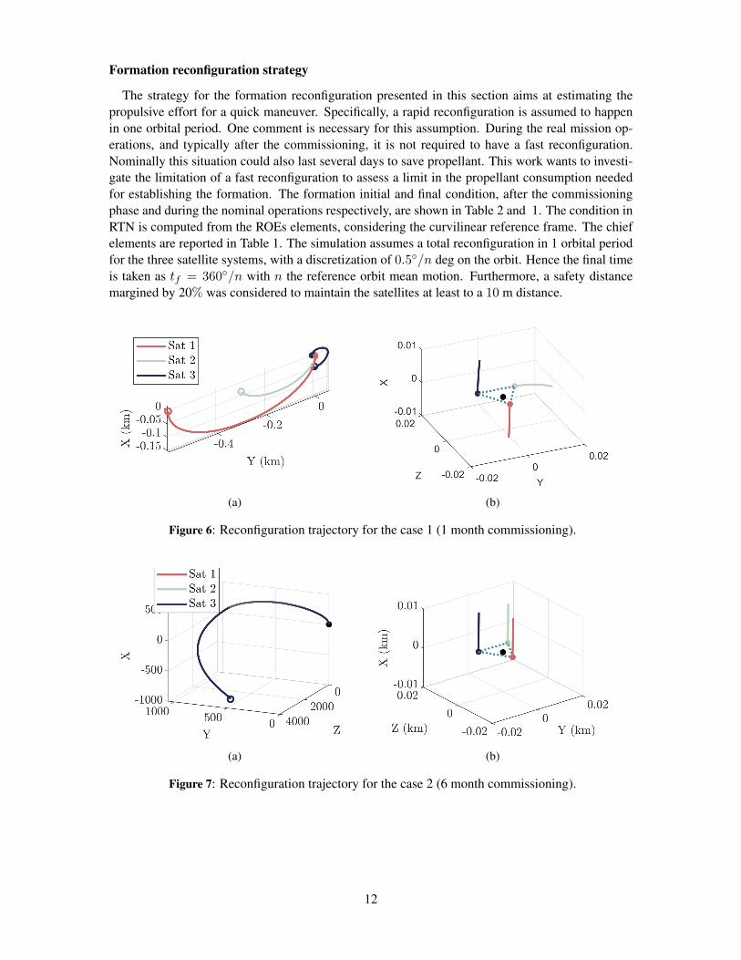
Formation reconfiguration strategy

The strategy for the formation reconfiguration presented in this section aims at estimating thepropulsive effort for a quick maneuver. Specifically, a rapid reconfiguration is assumed to happenin one orbital period. One comment is necessary for this assumption. During the real mission op-erations, and typically after the commissioning, it is not required to have a fast reconfiguration.Nominally this situation could also last several days to save propellant. This work wants to investi-gate the limitation of a fast reconfiguration to assess a limit in the propellant consumption neededfor establishing the formation. The formation initial and final condition, after the commissioningphase and during the nominal operations respectively, are shown in Table 2 and 1. The condition inRTN is computed from the ROEs elements, considering the curvilinear reference frame. The chiefelements are reported in Table 1. The simulation assumes a total reconfiguration in 1 orbital periodfor the three satellite systems, with a discretization of 0.5/n deg on the orbit. Hence the final timeis taken as tf = 360/n with n the reference orbit mean motion. Furthermore, a safety distancemargined by 20% was considered to maintain the satellites at least to a 10 m distance.

(a) (b)

Figure 6: Reconfiguration trajectory for the case 1 (1 month commissioning).

(a) (b)

Figure 7: Reconfiguration trajectory for the case 2 (6 month commissioning).

12

Figure 6 and 7 show the reconfiguration strategy for the two cases presented in the section Com-missioning phase. For the second case, with a longer commissioning phase, the satellites are fartherfrom the virtual reference point. For this reason, they will follow a very similar trajectory. Fig-ure 8 represents the relative trajectory of satellite 2 and 3 respect to satellite 1 to appreciate thedifferent trajectory followed. In these figures, the filled marker represents the target final position.The other marker instead, represents the initial condition before the reconfiguration maneuver. Theinitial separation with respect to the reference orbit is much more evident in the second case sincethe six-month commissioning produces a higher variation in the semi-major axis and eccentricity ofthe orbits. The satellites are reconfigured in a triangular formation, as shown in Figure 6-b and 7-b,around the reference virtual point on the nominal SSO orbit.

The collision avoidance is satisfied in both cases, as depicted in Figure 9 and Figure 10. Thosefigures represent the spacecraft inter-satellite distance. It is shown how for the entire formationreconfiguration, the satellites stay at more than 10 m from each other. Moreover, this stringentcondition is reached only at the final steps of the reconfiguration, when the formation tends to thenominal case, with a final inter-satellite distance of 13 m.

Figure 8: Reconfiguration trajectory for the case 2 (6 month commissioning). The relative trajectoryof satellites 2 and 3 are here represented with respect to the trajectory of satellite 1.

Figure 9: Inter-satellite distance evaluation during the reconfiguration manoeuvre (1 month com-missioning).

13

Figure 10: Inter-satellite distance evaluation during the reconfiguration manoeuvre (6 month com-missioning).

Finally, also the maneuvering plan is shown in Figure 11 and 12. In both cases, the maneu-vering plans provide an optimal strategy to correct at a certain time instant the trajectory, sav-ing propellant. In the first case, the satellites are positioned around the reference point such thatthe trajectory followed is quite different, and this results in a control strategy different for eachsatellite. In this case, the delta-v required by each satellites for the reconfiguration is respectively[0.9591 0.5925 1.790] mm/s. On the other hand, in the second case, it was shown that the tra-jectory followed is very similar. The maneuvering plan is almost equal among the satellites. Thissecond condition requires a delta-v of 5.7361 m/s for the reconfiguration.

Figure 11: Maneuvring plan evaluation for each satellite during the reconfiguration maneuvre (1month commissioning).

14

Figure 12: Maneuvring plan evaluation for each satellite during the reconfiguration maneuvre (6month commissioning).

CONCLUSION

In this paper, we show a fast approach to reconfigure a satellite formation after the orbital injec-tion. The maneuvering plan is defined via the optimization of the control problem in the convexform. This methodology allows a fast resolution of the system (∼ 3 s for both cases presented),by discretizing the problem in relatively few time instant. Moreover, the methodology applied, en-sures the application of a delta-v only at optimal time instants, saving propellant consumption. Inthe first framework, the results provide a fast and cheap reconfiguration, since, in a short commis-sioning phase, the difference in relative orbital parameters is small. On the other hand, the secondcase presented, implements a quite higher delta-v, this is mainly due to the constraint given on thelonger duration of the commissioning time. A fast reconfiguration is more expensive due to themore significant difference among the satellite elements and the reference orbit ones.

In both cases, the reconfiguration problem is approached as a minimization problem. The costfunction aims to minimize the total delta-v for the maneuvers. The explicit derivation of the con-straint from the system dynamics, initial conditions, and final conditions support the software im-plementation of the proposed strategy. A convex approach is computationally less expensive thanan optimization including the integration of the dynamics at each time step. This could also beenvisioned as a proper method to be put in the on-board software for formation maneuver imple-mentation. Moreover, the concept of a fast maneuver could be applied to formation maneuversduring the nominal mission phase, such as for the safety maneuver to switch to safe mode or toimplement a maneuver just after a possible failure in the system.

Further development of the methodology will include the uncertainties after the launcher injectionin the semi-major axis and the inclination. This will be managed with a Monte Carlo simulation togenerate the initial condition for the formation reconfiguration to the solver.

ACKNOWLEDGMENT

The project presented in this paper was carried out as part of the European Space Agency Contract(Contract No. 4000128576/19). The view expressed in this paper can in no way be taken to reflect

15

the official opinion of the European Space Agency.The work was co-founded by the European Space Agency (Contract No. 4000128576/19) andby the European Research Council (ERC) under the European Unions Horizon 2020 research andinnovation program (grant agreement No. 679086 COMPASS).The contribution of Dr. Gabriella Gaias is funded by the European Union’s Horizon 2020 researchand innovation program under the Marie-Sklodowska Curie grant ReMoVE (grant agreement No.793361).The authors acknowledge the contribution of Dr. Berthyl Duesmann and Dr. Itziar Bara, orbitalexperts at ESA European Space Research and Technology Centre (ESTEC).The authors also would like to acknowledge Dr. Miguel Piera’s support, from Airbus Space Espana,leading the contract.

REFERENCES

[1] G. Krieger, A. Moreira, H. Fiedler, I. Hajnsek, M. Werner, M. Younis, and M. Zink, “TanDEM-X:A satellite formation for high-resolution SAR interferometry,” IEEE Transactions on Geoscience andRemote Sensing, Vol. 45, No. 11, 2007, pp. 3317–3341, https://doi.org/10.1109/TGRS.2007.900693.

[2] S. Bandyopadhyay, R. Foust, G. P. Subramanian, S.-J. Chung, and F. Y. Hadaegh, “Review of formationflying and constellation missions using nanosatellites,” Journal of Spacecraft and Rockets, Vol. 53,No. 3, 2016, pp. 567–578, https://doi.org/10.2514/1.A33291.

[3] A. M. Zurita, I. Corbella, M. Martın-Neira, M. A. Plaza, F. Torres, and F. J. Benito, “To-wards a SMOS operational mission: SMOSOps-hexagonal,” IEEE Journal of Selected Top-ics in Applied Earth Observations and Remote Sensing, Vol. 6, No. 3, 2013, pp. 1769–1780,https://doi.org/10.1109/JSTARS.2013.2265600.

[4] Y. H. Kerr, A. Al-Yaari, N. Rodriguez-Fernandez, M. Parrens, B. Molero, D. Leroux, S. Bircher,A. Mahmoodi, A. Mialon, P. Richaume, et al., “Overview of SMOS performance in terms of globalsoil moisture monitoring after six years in operation,” Remote Sensing of Environment, Vol. 180, 2016,pp. 40–63, https://doi.org/10.1016/j.rse.2016.02.042.

[5] E. S. Agency, “Summary on ”ECMWF/ESA workshop on using low frequency passive microwavemeasurements in research and operational applications”,” 2017.

[6] M. Martin-Neira, “SMOS Follow-on - H,” L-band Continuation Workshop, CESBIO, Toulouse (France),28-30 November 2018.

[7] M. Martin-Neira, A. M. Zurita, M. A. Plaza, and F. J. Benito, “SMOS Follow-on Operational MissionConcept (SMOSops-H),” 2nd SMOS Science Conference, ESAC, Villanueva de la Canada, 25-29 May2015.

[8] A. W. Koenig and S. D’Amico, “Safe spacecraft swarm deployment and acquisition in perturbed near-circular orbits subject to operational constraints,” Acta Astronautica, Vol. 153, 2018, pp. 297–310,https://doi.org/10.1016/j.actaastro.2018.01.037.

[9] S. D’Amico, “Relative orbital elements as integration constants of Hill’s equations,” DLR, TN, 2005,pp. 05–08.

[10] G. Gaias, C. Colombo, and M. Lara, “Analytical Framework for Precise Relative Motion in LowEarth Orbits,” Journal of Guidance, Control, and Dynamics, Vol. 43, No. 5, 2020, pp. 915–927,https://doi.org/10.2514/1.G004716.

[11] M. Sabatini and G. B. Palmerini, “Linearized Formation-Flying Dynamics in a Per-turbed Orbital Environment,” 2008 IEEE Aerospace Conference, 2008, pp. 1–13,https://doi.org/10.1109/AERO.2008.4526271.

[12] C. Wei, S.-Y. Park, and C. Park, “Linearized dynamics model for relative motion under a J2-perturbedelliptical reference orbit,” International Journal of Non-Linear Mechanics, Vol. 55, 2013, pp. 55–69,https://doi.org/10.1016/j.ijnonlinmec.2013.04.016.

[13] S. Vaddi, K. T. Alfriend, S. Vadali, and P. Sengupta, “Formation establishment and reconfiguration usingimpulsive control,” Journal of Guidance, Control, and Dynamics, Vol. 28, No. 2, 2005, pp. 262–268,https://doi.org/10.2514/1.6687.

[14] M. Chernick and S. D’Amico, “New closed-form solutions for optimal impulsive control of spacecraftrelative motion,” Journal of Guidance, Control, and Dynamics, Vol. 41, No. 2, 2018, pp. 301–319,https://doi.org/10.2514/1.G002848.

16

[15] G. Gaias and S. D’Amico, “Impulsive maneuvers for formation reconfiguration using relative or-bital elements,” Journal of Guidance, Control, and Dynamics, Vol. 38, No. 6, 2015, pp. 1036–1049,https://doi.org/10.2514/1.G000189.

[16] S. Mitani and H. Yamakawa, “Continuous-thrust transfer with control magnitude and direction con-straints using smoothing techniques,” Journal of guidance, control, and dynamics, Vol. 36, No. 1, 2013,pp. 163–174, https://doi.org/10.2514/1.56882.

[17] S. Sarno, J. Guo, M. D’Errico, and E. Gill, “A guidance approach to satellite formation reconfig-uration based on convex optimization and genetic algorithms,” Advances in Space Research, 2020,https://doi.org/10.1016/j.asr.2020.01.033.

[18] L. M. Steindorf, S. D’Amico, J. Scharnagl, F. Kempf, and K. Schilling, “Constrained low-thrust satelliteformation-flying using relative orbit elements,” 27th AAS/AIAA Space Flight Mechanics Meeting, 2017.

[19] P. M. Pardalos, “Convex optimization theory,” Optimization Methods and Software, Vol. 25, No. 3,2010, pp. 487–487, https://doi.org/10.1080/10556781003625177.

[20] B. Acikmese, D. Scharf, F. Hadaegh, and E. Murray, “A convex guidance algorithm for formationreconfiguration,” AIAA Guidance, Navigation, and Control Conference and Exhibit, 2006, p. 6070.

[21] D.-W. Gim and K. T. Alfriend, “State transition matrix of relative motion for the perturbed noncircularreference orbit,” Journal of Guidance, Control, and Dynamics, Vol. 26, No. 6, 2003, pp. 956–971.

[22] D. Izzo, M. Sabatini, and C. Valente, “A new linear model describing formation flying dynamics underJ2 effects,” Proceedings of the 17th AIDAA National Congress, Vol. 1, 2003, pp. 15–19.

[23] G. Gaias, J.-S. Ardaens, and C. Colombo, “Precise Line-of-Sight Modelling for Angles-Only RelativeNavigation,” Advances in Space Research, Article in Advance (published online 10 Jun 2020), Vol. ISSN0273-1177, 2020, https://doi.org/10.1016/j.asr.2020.05.048 (open access).

[24] M. C. Grant and S. P. Boyd, “Graph implementations for nonsmooth convex programs,” Recent ad-vances in learning and control, pp. 95–110, Springer, 2008.

[25] M. Grant, S. Boyd, and Y. Ye, “CVX: Matlab software for disciplined convex programming, version2.0 beta,” 2013.

[26] M. Wermuth, G. Gaias, and S. D’Amico, “Safe Picosatellite Release from a Small Satellite Carrier,”Journal of Spacecraft and Rockets, Vol. 52, No. 5, 2015, pp. 1338–1347, 10.2514/1.A33036.

17