aass learning systems lab, Örebro...
TRANSCRIPT
AASS Learning Systems Lab, Örebro University
Matteo Reggente and Achim J. Lilienthal
Contents
1. Background
2. Experimental Setup
3. Gas Distribution Model
4. Experiments and Results
5. Ongoing and Future Work

Contents
Background
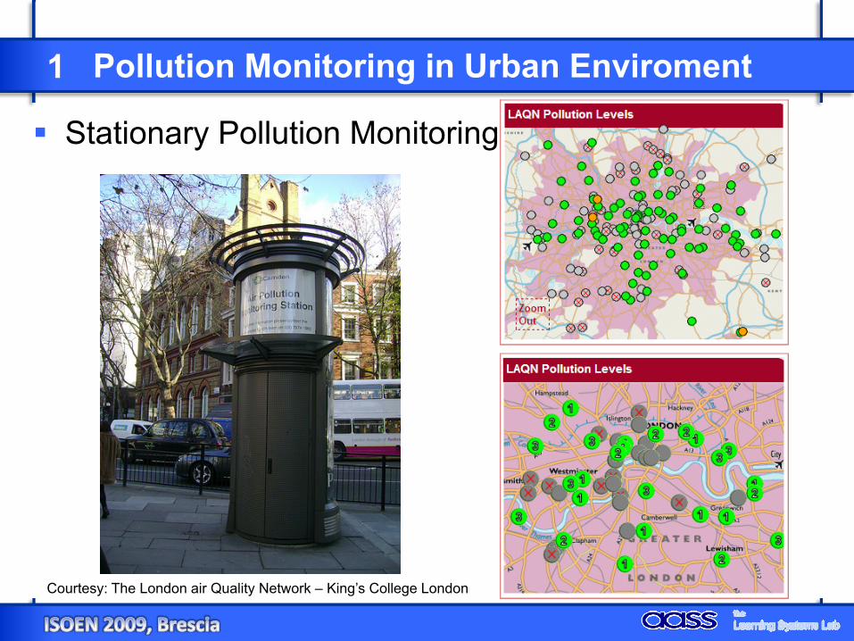
1 Pollution Monitoring in Urban Enviroment
Stationary Pollution Monitoring
Courtesy: The London air Quality Network – King’s College London
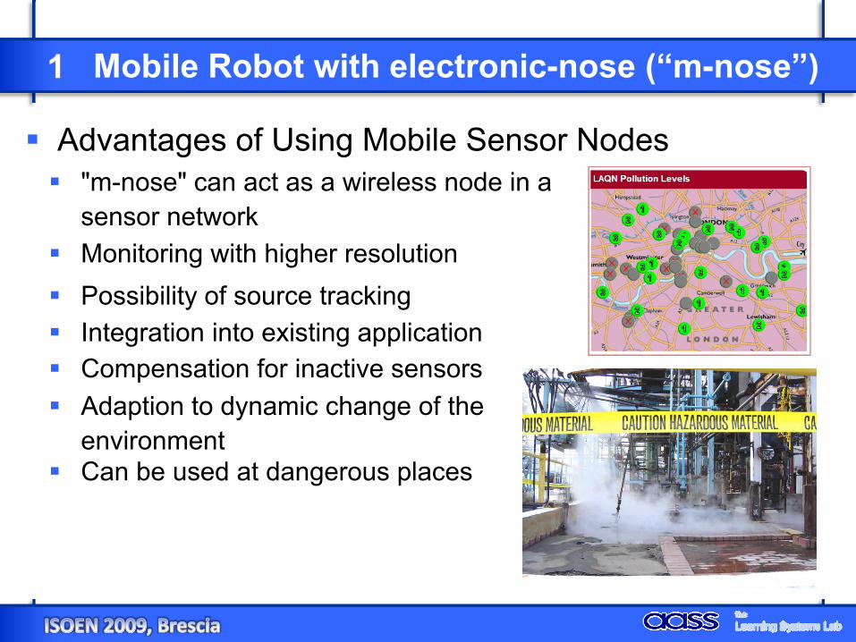
1 Mobile Robot with electronic-nose (“m-nose”)
Advantages of Using Mobile Sensor Nodes"m-nose" can act as a wireless node in a sensor network Monitoring with higher resolutionPossibility of source trackingIntegration into existing applicationCompensation for inactive sensorsAdaption to dynamic change of the environmentCan be used at dangerous places
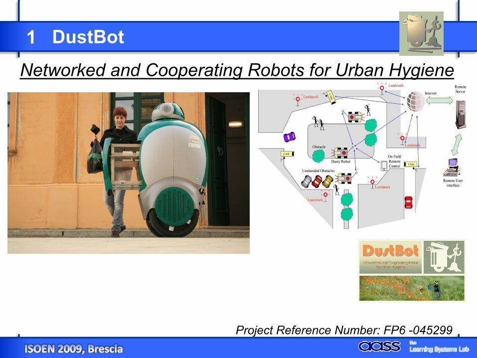
1 DustBot
Project Reference Number: FP6 -045299
Networked and Cooperating Robots for Urban Hygiene
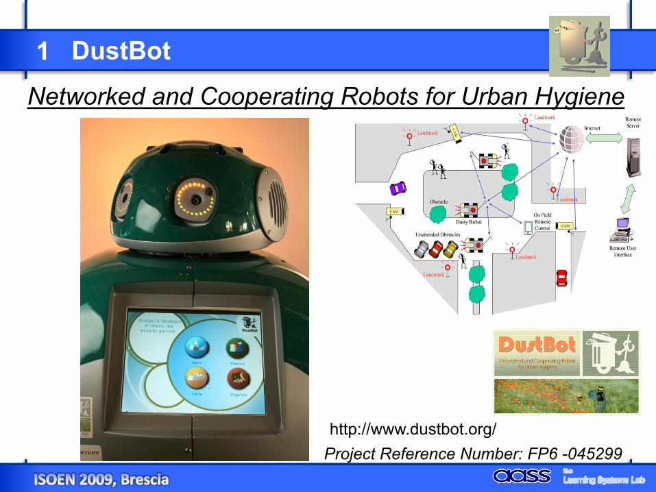
1 DustBot
Project Reference Number: FP6 -045299
Networked and Cooperating Robots for Urban Hygiene
http://www.dustbot.org/
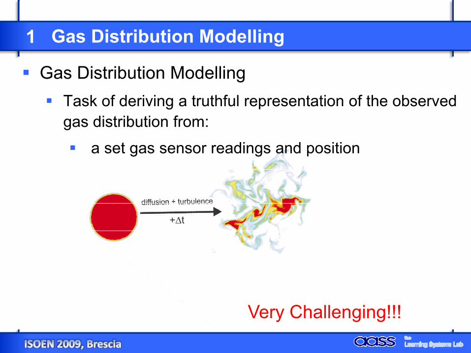
1 Gas Distribution Modelling
Gas Distribution ModellingTask of deriving a truthful representation of the observed gas distribution from:
a set gas sensor readings and position
Very Challenging!!!
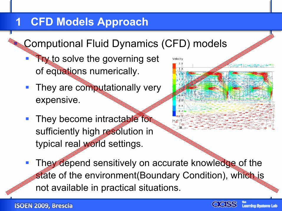
1 CFD Models Approach
Computional Fluid Dynamics (CFD) modelsTry to solve the governing set of equations numerically.
They are computationally very expensive.
They become intractable for sufficiently high resolution in typical real world settings.
They depend sensitively on accurate knowledge of the state of the environment(Boundary Condition), which is not available in practical situations.
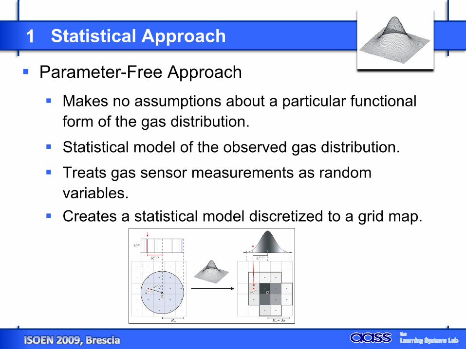
1 Statistical Approach
Parameter-Free ApproachMakes no assumptions about a particular functional form of the gas distribution.Statistical model of the observed gas distribution.Treats gas sensor measurements as random variables.Creates a statistical model discretized to a grid map.

1 Related Work
3D – Gas Tracking with Blimp
H. Ishida et al., “Three-Dimensional Gas/Odor Plume Tracking with Blimp,” in Proc. ICEE, 2004.
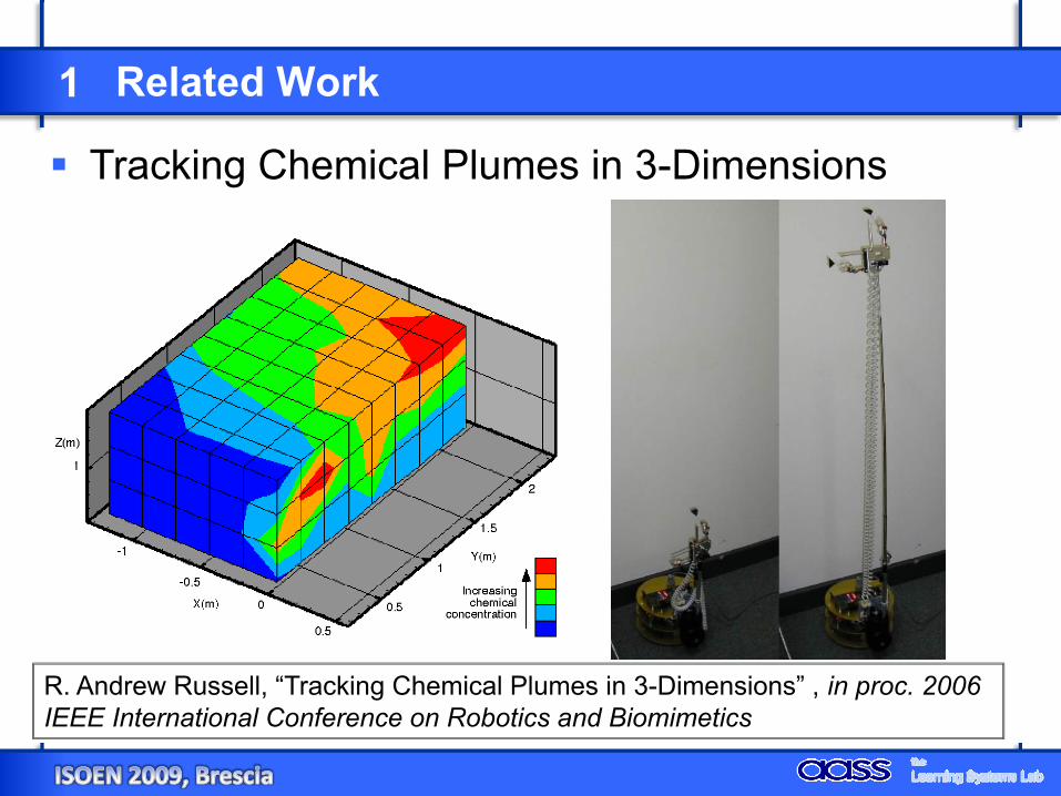
1 Related Work
Tracking Chemical Plumes in 3-Dimensions
R. Andrew Russell, “Tracking Chemical Plumes in 3-Dimensions” , in proc. 2006 IEEE International Conference on Robotics and Biomimetics
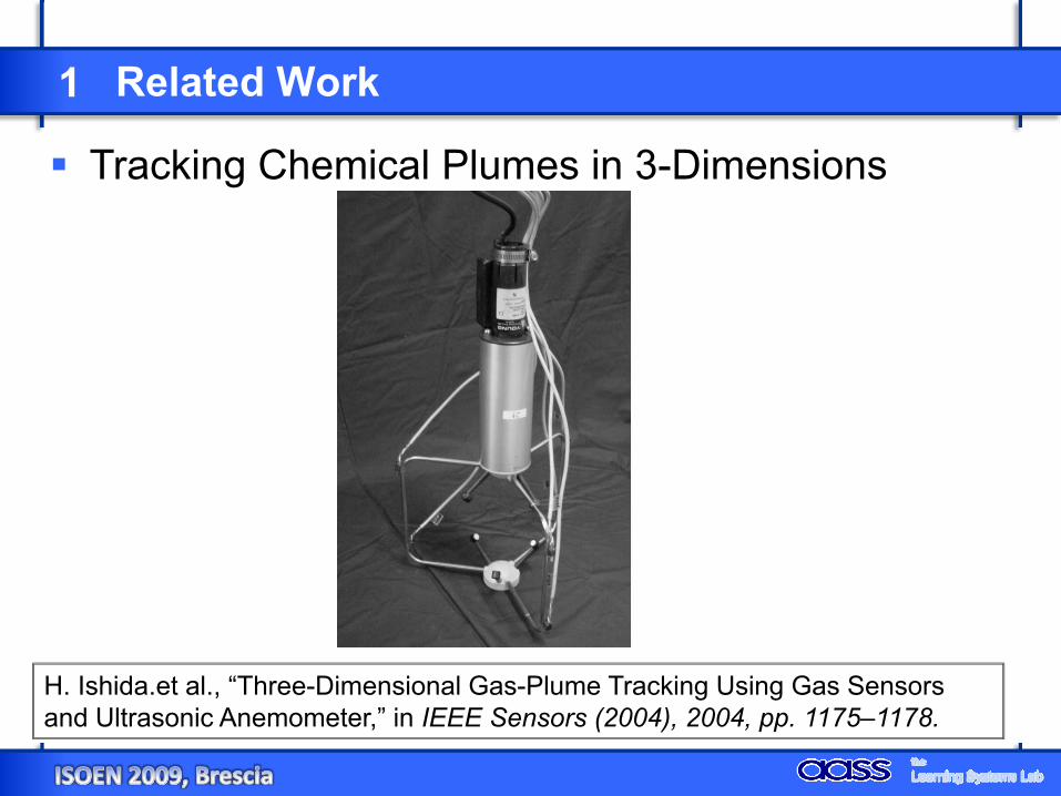
1 Related Work
Tracking Chemical Plumes in 3-Dimensions
H. Ishida.et al., “Three-Dimensional Gas-Plume Tracking Using Gas Sensors and Ultrasonic Anemometer,” in IEEE Sensors (2004), 2004, pp. 1175–1178.
Contents
Experimental Setup
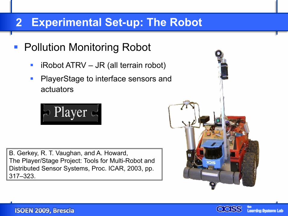
2 Experimental Set-up: The Robot
Pollution Monitoring RobotiRobot ATRV – JR (all terrain robot)
PlayerStage to interface sensors and actuators
B. Gerkey, R. T. Vaughan, and A. Howard, The Player/Stage Project: Tools for Multi-Robot and Distributed Sensor Systems, Proc. ICAR, 2003, pp. 317–323.
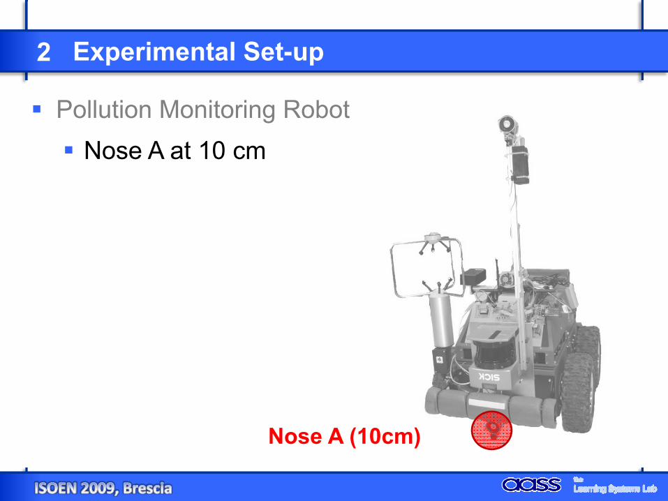
2 Experimental Set-up
Pollution Monitoring Robot
Nose A (10cm)
Nose A at 10 cm
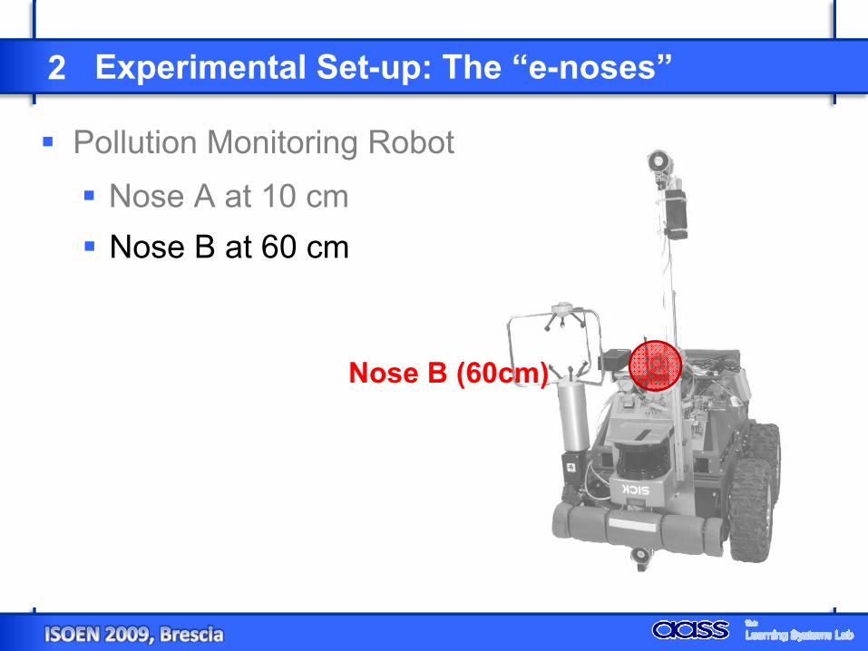
2 Experimental Set-up: The “e-noses”
Pollution Monitoring RobotNose A at 10 cm
Nose B (60cm)
Nose B at 60 cm
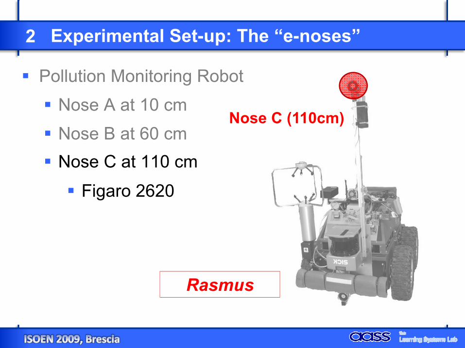
2 Experimental Set-up: The “e-noses”
Pollution Monitoring RobotNose A at 10 cmNose B at 60 cm
Nose C (110cm)
Nose C at 110 cm
Figaro 2620
Rasmus
Contents
Gas Distribution Model
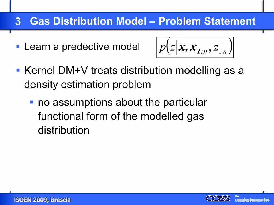
3 Gas Distribution Model – Problem Statement
Learn a predective model ( )nzzp :1,n:1xx,
Kernel DM+V treats distribution modelling as a density estimation problem
no assumptions about the particular functional form of the modelled gas distribution
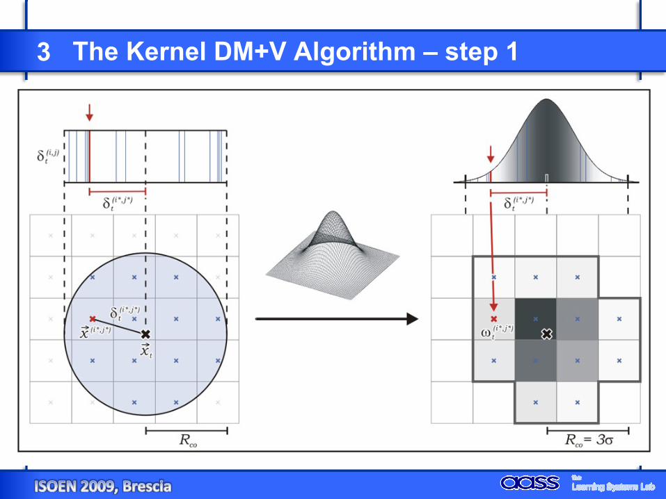
3 The Kernel DM+V Algorithm – step 1
ωi(k)(σ)
Weights represent the importance of
sensor measurement iat grid cell (k).
They are computed using
a multivariate Gaussian
kernel.
ωi(k)(σ) = N (|xi – x(k)|,σ)
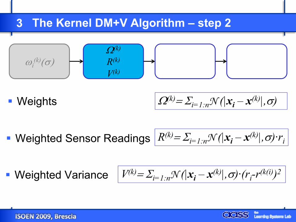
3 The Kernel DM+V Algorithm – step 2
ωi(k)(σ)
Ω(k)
R(k)
V(k)
Weights
Weighted Variance
Ω(k)= Σi=1:nN (|xi – x(k)|,σ)
R(k)= Σi=1:nN (|xi – x(k)|,σ)·riWeighted Sensor Readings
V(k)= Σi=1:nN (|xi – x(k)|,σ)·(ri-r(k(i))2
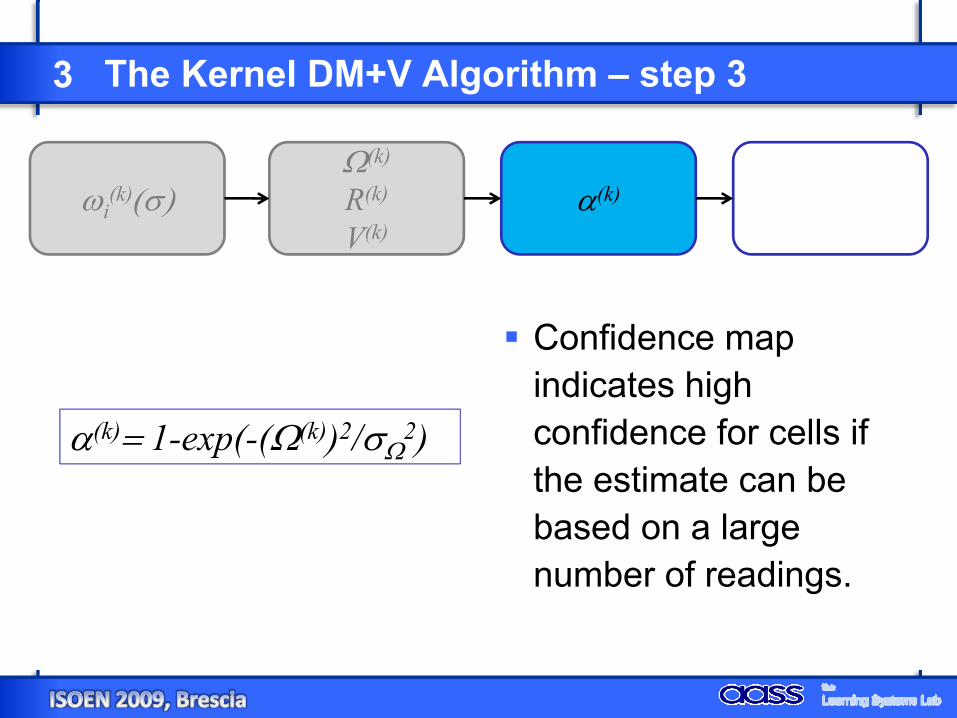
3 The Kernel DM+V Algorithm – step 3
ωi(k)(σ)
Ω(k)
R(k)
V(k)α(k)
Confidence map indicates high confidence for cells if the estimate can be based on a large number of readings.
α(k)= 1-exp(-(Ω(k))2/σΩ2)
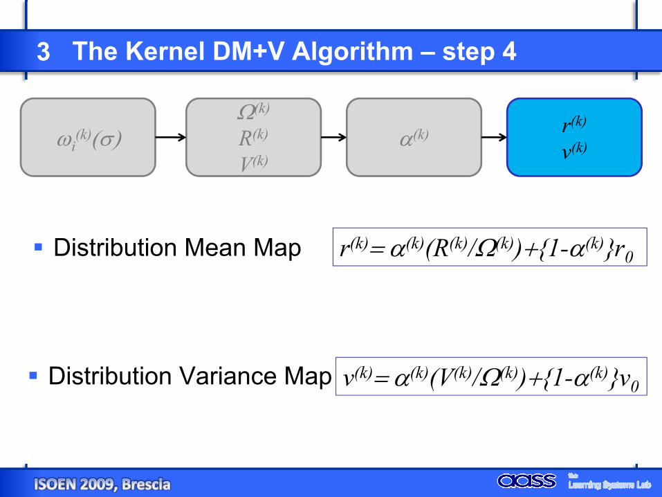
3 The Kernel DM+V Algorithm – step 4
ωi(k)(σ)
Ω(k)
R(k)
V(k)α(k) r(k)
v(k)
Distribution Mean Map
Distribution Variance Map
r(k)= α(k)(R(k)/Ω(k))+{1-α(k)}r0
v(k)= α(k)(V(k)/Ω(k))+{1-α(k)}v0
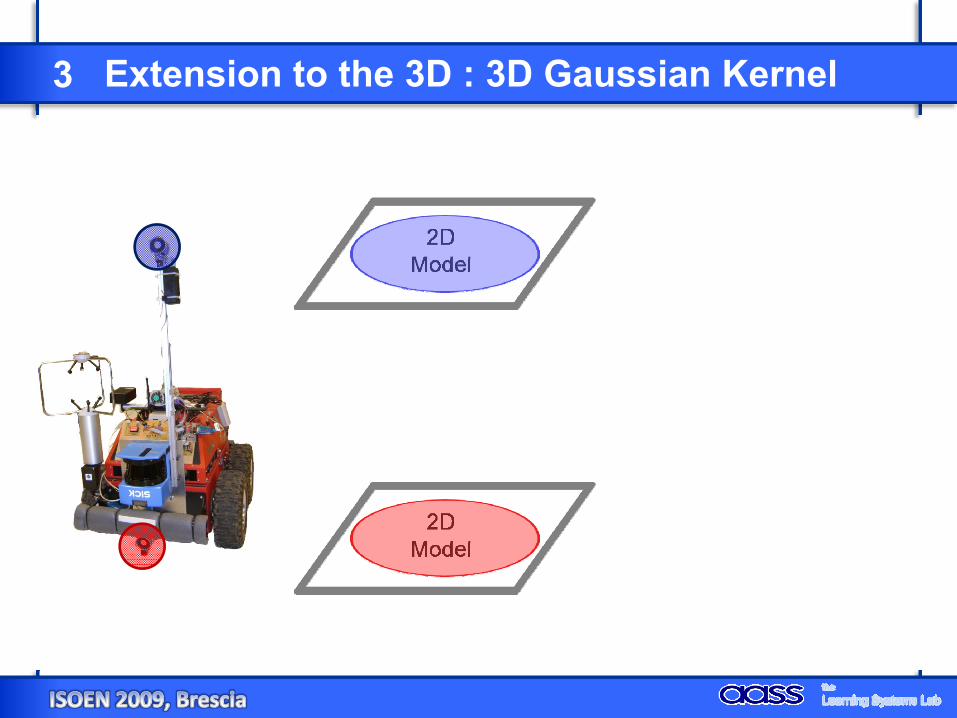
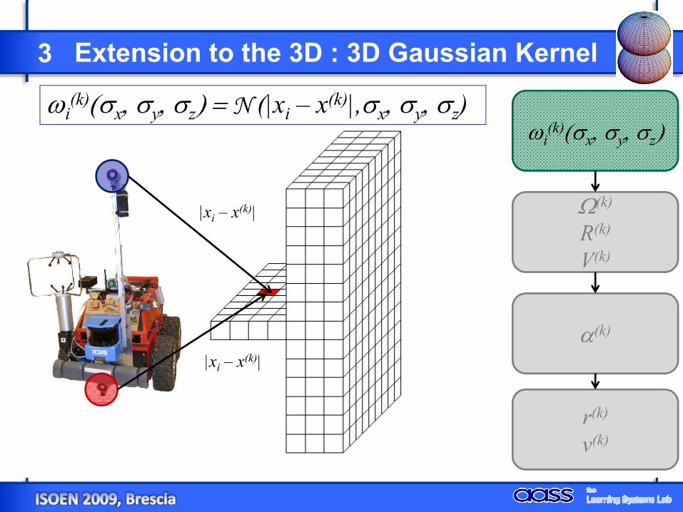
3 Extension to the 3D : 3D Gaussian Kernel
2D Model
2D Model
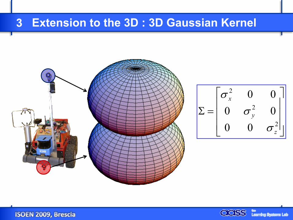
3 Extension to the 3D : 3D Gaussian Kernel
⎥⎥⎥
⎦
⎤
⎢⎢⎢
⎣
⎡
=Σ2
2
2
000000
z
y
x
σσ
σ
3 Extension to the 3D : 3D Gaussian Kernel
ωi(k)(σx, σy, σz) = N (|xi – x(k)|,σx, σy, σz)
ωi(k)(σx, σy, σz)
Ω(k)
R(k)
V(k)
α(k)
r(k)
v(k)
|xi – x(k)|
|xi – x(k)|

3 Extension to the 3D : 3D Gaussian Kernel
ωi(k)(σx, σy, σz)
Ω(k) )(σx, σy, σz)R(k) )(σx, σy, σz)V(k) )(σx, σy, σz)
α(k)
r(k)
v(k)
Weights
Weighted Variance
Ω(k) = Σi=1:nN (|xi – x(k)|, σx, σy, σz)
R(k) = Σi=1:nN (|xi – x(k)|, σx, σy, σz)·ri
Weighted Sensor Readings
V(k) = Σi=1:nN (|xi – x(k)|, σx, σy, σz)·(ri-r(k(i))2
3 Extension to the 3D : 3D Gaussian Kernel
ωi(k)(σx, σy, σz)
Ω(k) )(σx, σy, σz)R(k) )(σx, σy, σz)V(k) )(σx, σy, σz)
α(k) )(σx, σy, σz)
r(k)
v(k)
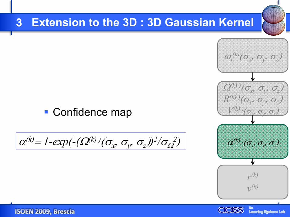
Confidence map
α(k)= 1-exp(-(Ω(k) )(σx, σy, σz))2/σΩ2)
3 Extension to the 3D : 3D Gaussian Kernel
ωi(k)(σx, σy, σz)
Ω(k) )(σx, σy, σz)R(k) )(σx, σy, σz)V(k) )(σx, σy, σz)
α(k) )(σx, σy, σz)
r(k)
v(k)
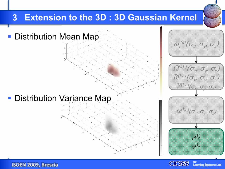
Distribution Mean Map
Distribution Variance Map
Contents
Experiments and Results
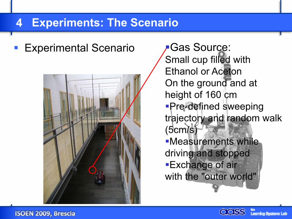
4 Experiments: The Scenario
Experimental Scenario Gas Source:Small cup filled with Ethanol or AcetonOn the ground and at height of 160 cmPre-defined sweeping
trajectory and random walk (5cm/s)Measurements while
driving and stoppedExchange of air
with the "outer world"
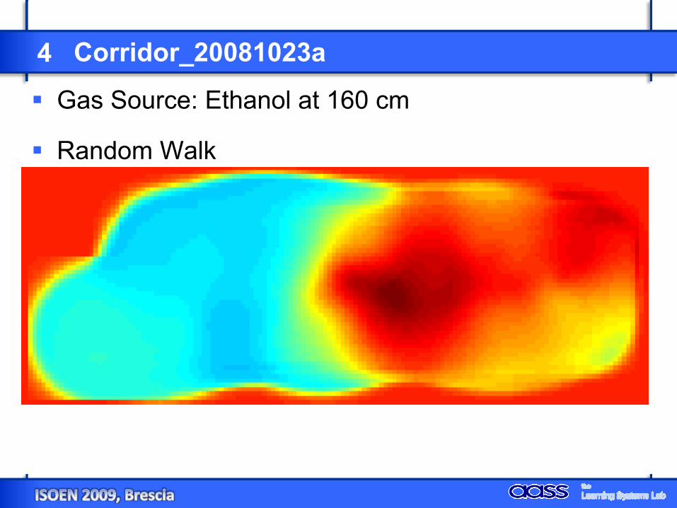
4 Corridor_20081023a
Gas Source: Ethanol at 160 cm
Random Walk
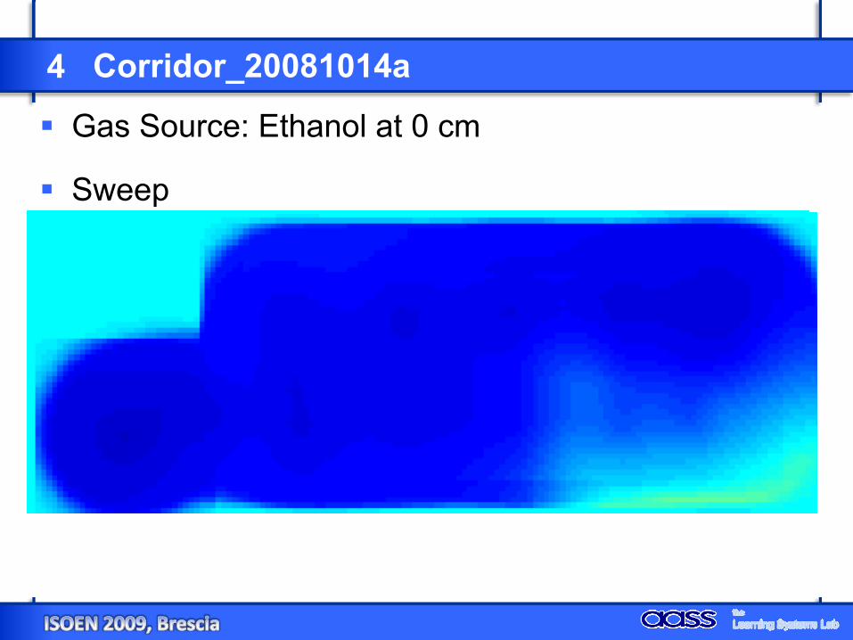
4 Corridor_20081014a
Gas Source: Ethanol at 0 cm
Sweep
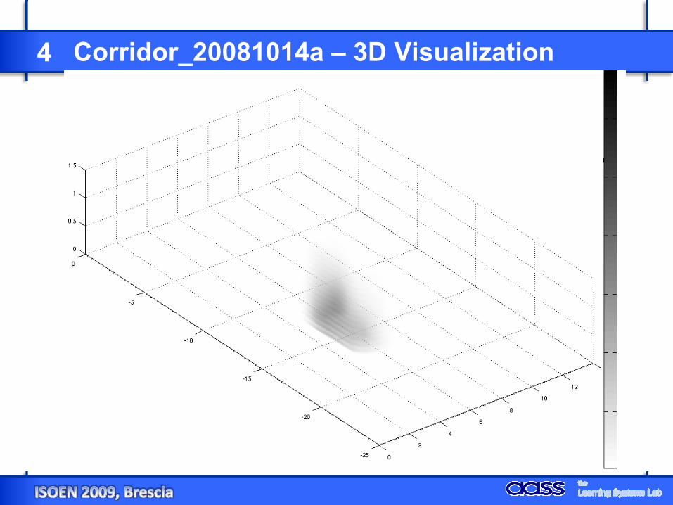
4 Corridor_20081014a – 3D Visualization
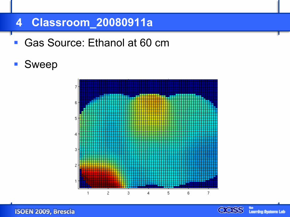
4 Classroom_20080911a
Gas Source: Ethanol at 60 cm
Sweep
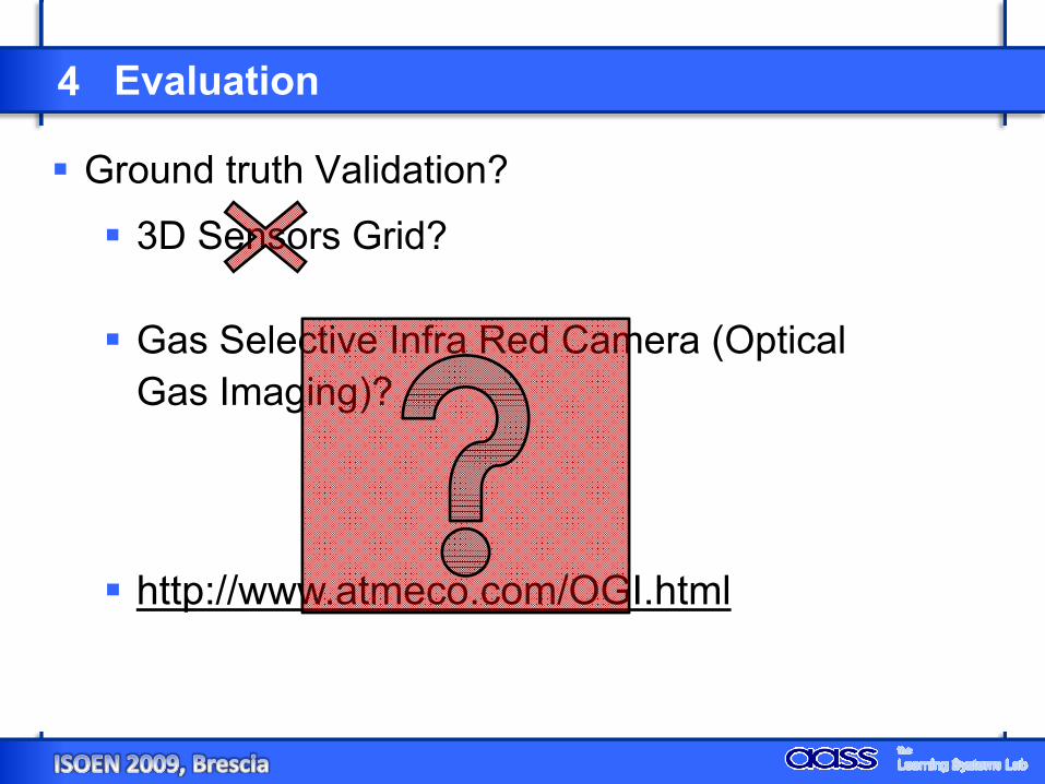
4 Evaluation
Ground truth Validation?
3D Sensors Grid?
Gas Selective Infra Red Camera (Optical Gas Imaging)?
http://www.atmeco.com/OGI.html

4 Statistical Evaluation
2D Model

4 Statistical Evaluation
Kullback-Leibler (KL) divergence
( ) ∫−= dxxpxqxpqpKL)()(ln)(
ModelledDistribution
Unknown Distribution
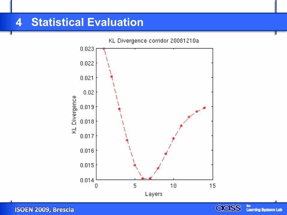
4 Statistical Evaluation

4 Statistical Evaluation
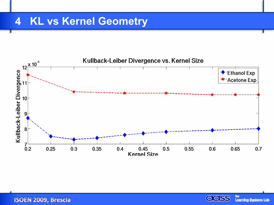
4 KL vs Kernel Geometry

Contents
Ongoing and Future Work
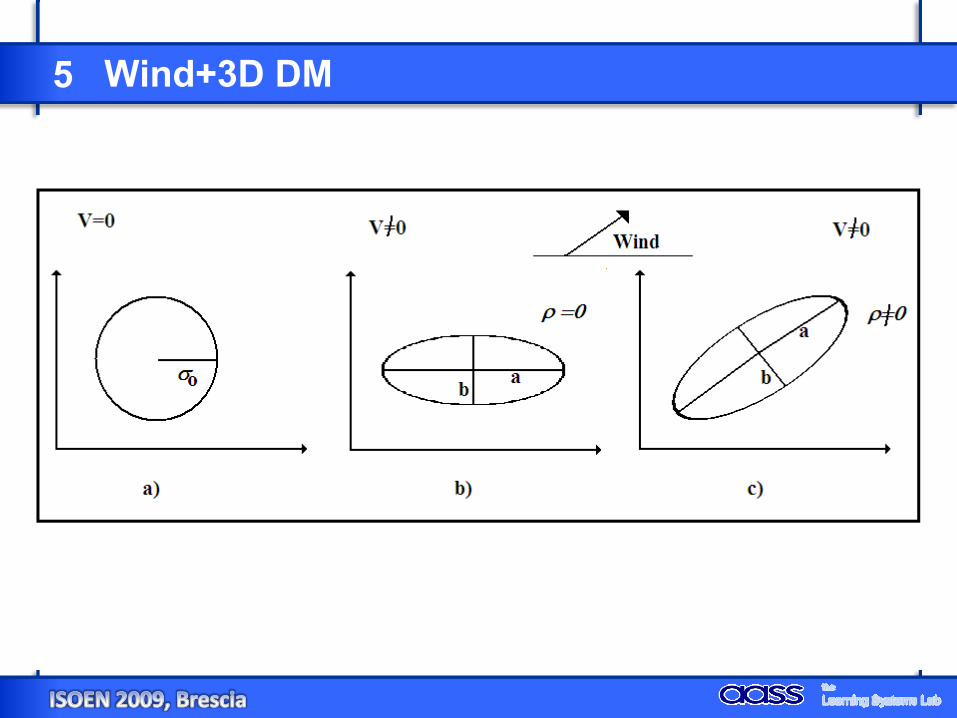
5 Wind+3D DM
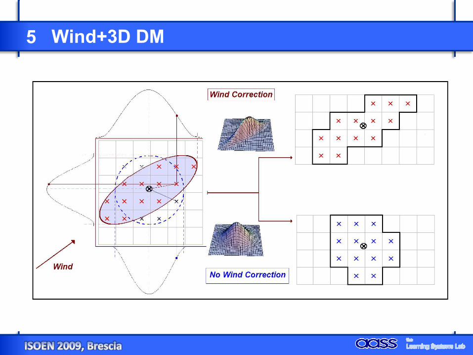
5 Wind+3D DM