ab - tcs.hut.fi · tkk reports in information and computer science ... 5 case study: falcon 24 ......

TKK Reports in Information and Computer Science

Espoo 2008 TKK-ICS-R3

MODEL CHECKING TIMED SAFETY INSTRUMENTED

SYSTEMS

Jussi Lahtinen

AB TEKNILLINEN KORKEAKOULU

TEKNISKA HÖGSKOLAN

HELSINKI UNIVERSITY OF TECHNOLOGY

TECHNISCHE UNIVERSITÄT HELSINKI

UNIVERSITE DE TECHNOLOGIE D’HELSINKI

TKK Reports in Information and Computer Science

Espoo 2008 TKK-ICS-R3

MODEL CHECKING TIMED SAFETY INSTRUMENTED

SYSTEMS

Jussi Lahtinen

Helsinki University of Technology

Faculty of Information and Natural Sciences

Department of Information and Computer Science

Teknillinen korkeakoulu

Informaatio- ja luonnontieteiden tiedekunta

Tietojenkasittelytieteen laitos

Distribution:

Helsinki University of Technology

Faculty of Information and Natural Sciences

Department of Information and Computer Science

P.O.Box 5400

FI-02015 TKK

FINLAND

URL: http://ics.tkk.fi

Tel. +358 9 451 1

Fax +358 9 451 3369

E-mail: [email protected]

©c Jussi Lahtinen

ISBN 978-951-22-9444-2 (Print)

ISBN 978-951-22-9445-9 (Online)

ISSN 1797-5034 (Print)

ISSN 1797-5042 (Online)

URL: http://www.otalib.fi/tkk/edoc/

TKK ICS

Espoo 2008

ABSTRACT: Defects in safety-critical software systems can cause large eco-nomical and other losses. Often these systems are far too complex to be testedextensively. In this work a formal verification technique called model check-ing is utilized. In the technique, a mathematical model is created that cap-tures the essential behaviour of the system. The specifications of the systemare stated in some formal language, usually temporal logic. The behaviourof the model can then be checked exhaustively against a given specification.

This report studies the Falcon arc protection system engineered by UTUOy, which is controlled by a single programmable logic controller (PLC).Two separate models of the arc protection system are created. Both mod-els consist of a network of timed automata. In the first model, the controlleroperates in discrete time steps at a specific rate. In the second model, the con-troller operates at varying frequency in continuous time. Five system spec-ifications were formulated in timed computation tree logic (TCTL). Usingthe model checking tool Uppaal both models were verified against all fivespecifications.

The processing times of the verification are measured and presented. Thediscrete-time model has to be abstracted a lot before it can be verified in areasonable time. The continuous-time model, however, covered more be-haviour than the system to be modelled, and could still be verified in a mod-erate time period. In that sense, the continuous-time model is better thanthe discrete-time model.

The main contributions of this report are the model checking of a safetyinstrumented system controlled by a PLC, and the techniques used to de-scribe various TCTL specifications in Uppaal. The conclusion of the work isthat model checking of timed systems can be used in the verification of safetyinstrumented systems.

KEYWORDS: safety instrumented systems, model checking, real-time, Up-paal

CONTENTS

List of Figures vii

1 Introduction 11.1 Model Checking . . . . . . . . . . . . . . . . . . . . . . . . 11.2 Work Description . . . . . . . . . . . . . . . . . . . . . . . . 21.3 Outline of the Work . . . . . . . . . . . . . . . . . . . . . . . 2

2 Model Checking of Timed Systems 22.1 Timed Automata . . . . . . . . . . . . . . . . . . . . . . . . 4

2.1.1 Formal Semantics . . . . . . . . . . . . . . . . . . . 52.1.2 Decision Problems in Timed Automata . . . . . . . . 72.1.3 Parallel Composition of Timed Automata . . . . . . . 82.1.4 Symbolic Semantics, Regions and Zones . . . . . . . 102.1.5 Difference Bound Matrices . . . . . . . . . . . . . . 12

2.2 Temporal Logic with Real Time . . . . . . . . . . . . . . . . 132.2.1 Computation Tree Logic . . . . . . . . . . . . . . . . 142.2.2 Timed Computation Tree Logic . . . . . . . . . . . . 15

2.3 Model Checking Tool Uppaal . . . . . . . . . . . . . . . . . 162.3.1 Modelling in Uppaal . . . . . . . . . . . . . . . . . . 172.3.2 Verification in Uppaal . . . . . . . . . . . . . . . . . 18

3 Timed Safety Instrumented Systems 193.1 Programmable Logic Controller . . . . . . . . . . . . . . . . 193.2 Safety Instrumented Systems . . . . . . . . . . . . . . . . . . 20

4 Modelling Systems with Timed Automata 214.1 Modelling Real-Time Communication Protocols . . . . . . . 214.2 Modelling Real-Time Controllers . . . . . . . . . . . . . . . 234.3 Other Real-Time Research . . . . . . . . . . . . . . . . . . . 24

5 Case Study: Falcon 245.1 The Falcon Arc Protection System . . . . . . . . . . . . . . . 245.2 System Environment Description . . . . . . . . . . . . . . . 255.3 Discrete-time Model . . . . . . . . . . . . . . . . . . . . . . 27

5.3.1 The Falcon Control Unit . . . . . . . . . . . . . . . . 285.3.2 Primary Breakers . . . . . . . . . . . . . . . . . . . . 295.3.3 Secondary Breakers . . . . . . . . . . . . . . . . . . . 30

5.4 Falcon: Continuous-time Model . . . . . . . . . . . . . . . . 305.4.1 The Falcon Control Unit . . . . . . . . . . . . . . . . 315.4.2 Primary Breakers . . . . . . . . . . . . . . . . . . . . 315.4.3 Secondary Breakers . . . . . . . . . . . . . . . . . . . 325.4.4 The Environment Model . . . . . . . . . . . . . . . 33

5.5 Checked Properties . . . . . . . . . . . . . . . . . . . . . . . 345.6 Conclusions of the Models . . . . . . . . . . . . . . . . . . . 36

6 Results 37

7 Conclusions 40

CONTENTS v

References 41

Appendices 46

A Falcon case: Discrete-time Model Related Code 46

B Falcon case: Continuous-time Model Related Code 50

C Falcon Case: The Discrete-time Simplified Model 52

D Falcon Case: The Continuous-time Simplified Model 55

vi CONTENTS

LIST OF FIGURES

1 A finite state automaton . . . . . . . . . . . . . . . . . . . . . 32 A timed automaton . . . . . . . . . . . . . . . . . . . . . . . 53 A timed automaton with invariant constraints . . . . . . . . . 54 Regions of a system . . . . . . . . . . . . . . . . . . . . . . . 115 The zone graph of the timed automaton in Figure 3 . . . . . 126 An observer automaton in Uppaal . . . . . . . . . . . . . . . 187 A TON timer with inputs IN and PT, and outputs Q and ET . 208 Functionality of a TON timer . . . . . . . . . . . . . . . . . 209 The Falcon architecture . . . . . . . . . . . . . . . . . . . . 2610 Falcon master unit logic of the example case . . . . . . . . . 2711 The Falcon system model with discrete time . . . . . . . . . . 2812 The discrete-time breaker model . . . . . . . . . . . . . . . . 3013 The discrete-time secondary breaker model . . . . . . . . . . 3014 The falcon system of the continuous-time model. . . . . . . . 3115 The continuous-time model of the breaker . . . . . . . . . . 3216 The secondary breaker model in continuous-time . . . . . . . 3217 The continuous-time environment model . . . . . . . . . . . 3318 The observer automaton used in property 3 in the continuous-

time case . . . . . . . . . . . . . . . . . . . . . . . . . . . . 3519 An observer automaton for discrete-time . . . . . . . . . . . . 3520 An observer automaton for continuous-time model . . . . . . 3621 The observer automaton used in Property 5 . . . . . . . . . . 3722 The Falcon control unit of the simplified discrete-time model 5223 The Falcon control unit of the simplified continuous-time

model . . . . . . . . . . . . . . . . . . . . . . . . . . . . . . 55

LIST OF FIGURES vii

LIST OF SYMBOLS AND ABBREVIATIONS

{d} The fractional part of d⌊d⌋ The integer part of dN The set of natural numbersR+ The set of non-negative real numbersR

C The set of clock valuationsA Temporal logic path quantifier: for all computation pathsE Temporal logic path quantifier: for some computation pathU Temporal logic operator: untilX Temporal logic operator: next timeBDD Binary decision diagramCCS Calculus of Communicating SystemsCTL Computation tree logicDBM Difference bound matrixFBD Function block diagramIEC International Electrotechnical CommissionIL Instruction listLD Ladder diagramPLC Programmable logic controllerSFC Structured function chartSIS Safety instrumented systemST Structured textTCTL Timed computation tree logicTON Timer on delayUTU Urho Tuominen Oy

viii LIST OF FIGURES

1 INTRODUCTION

Software plays an increasing role in safety-critical applications where an in-correct behaviour could lead to significant economical, environmental orpersonnel losses. Thus, it is imperative that these safety-critical systems con-form to their functional requirements. Testing is regularly used to ensurethat the requirements are met. Testing can not, however, show the absenceof software bugs, only their presence. If the system functionality has to beverified, some much more powerful method is needed.

1.1 Model Checking

Model checking [20] is an automatic technique for verifying hardware andsoftware designs. Other, more traditional system verification techniques in-clude simulation, testing, and deductive reasoning [20]. Deductive reasoningnormally means the use of axioms and proof rules to prove the correctnessof systems. Deductive reasoning techniques are often difficult and require alot of manual intervention. On the other hand, validation techniques basedon extensive testing or simulation can easily miss errors when the number ofpossible states of the system is very large. Model checking requires no usersupervision and always produces a counterexample when the design fails tosatisfy some checked property.

Model checking consists of modeling, specification, and verification. Firstly,the design under investigation has to be converted into a formalism under-stood by the used model checking tool. This means that the system behaviouris depicted in a modeling language. The model should comprise the essentialproperties of the system, and at the same time abstract away from unimpor-tant details that only complicate the verification process [20].

Secondly, the system has some properties it must satisfy. These properties,also called specifications, are usually given in some logical formalism. Forhardware and software designs, it is typical to use temporal logic [20], whichcan express the requirements for system behaviour over time.

After modeling and specification, only the fully automatic model checkerpart remains. If the design meets the desired properties, the verification toolwill state that the specification is true. In case of a design flaw or an incorrectmodeling or specification, a counterexample will be generated. A counterex-ample presents a legal execution sequence in the model that is not allowedby a specification. The analysis of the counterexample is usually impossibleto do automatically and thus involves human assistance. For example, it isimpossible for a computer program to decide whether the model or the spec-ification is incorrect. The counterexample can help the designer find theerrors in the specifications, in the design or in the model.

There are several model checking techniques. Many of them suffer fromthe state explosion problem [46]. State explosion results from the fact that

1 INTRODUCTION 1

the number of states in a system grows exponentially as the size of the modelincreases. Although the system is still finite, model checking might be toocomplex for even state-of-the-art computers. No fully satisfactory solution tothis problem has yet been found, although symbolic representation of thestate space using BDDs or reducing the needed state space using abstractionhave been found useful [17, 46]. Partial order reduction [24, 46, 20] is alsoa typical state space reduction method. Bounded model checking [9, 10] at-tempts to avoid the state explosion problem by bounding the counterexamplelength. Nevertheless, model checking is likely to prove an invaluable tool toverify system requirements or design.

1.2 Work Description

In this work, a real-time safety-critical system is modelled as a network oftimed automata [8]. Furthermore, the model is verified against five proper-ties using the model checking tool Uppaal. Timed automata are chosen asthe basis of the model, since the system is very dependent on correct timing.The theory of timed automata provides a framework to model and verify real-time systems.

The checked system is a safety instrumented system (SIS) that is controlledby a single programmable logic controller (PLC). The purpose of the systemis to cut electricity from a protected area, if an electric arc is observed. Be-cause of the complexity of the system, standard testing can not guarantee thecorrect functioning.

1.3 Outline of the Work

The rest of this work is organized as follows. In Section 2 timed automata areintroduced and the model checking methodology of this work is presented.In Section 3 the use of programmable logic controllers in timed safety instru-mented systems is discussed. A survey of related research is in Section 4. Thecase study of this work is presented in Section 5, where two different modelsof the system are shown. The results of the verification of the models are inSection 6. Finally, the conclusions of the work are in Section 7.

2 MODEL CHECKING OF TIMED SYSTEMS

Model checking methods often use automata as their primary modellingstructure. The automata can be finite state automata, timed automata, Büchiautomata or of some other automata class depending on the employed modelchecking method. Automata provide a way to describe the behaviour of themodelled system efficiently and precisely. Also, the modelling of specifica-tions by automata is possible. This provides a useful model checking ap-proach of a system. The specification automaton and the automaton of thesystem can be run in parallel. Usually model checking tools create a parallelcomposition of the system automaton and the negation of the specification

2 2 MODEL CHECKING OF TIMED SYSTEMS

automaton. If the created automaton is not empty, the specification is notmet by the system. A counterexample can be easily extracted from the paral-lel composition.

A finite automaton [20] is a mathematical model of a system that has aconstant amount of memory that does not depend on the size of the input.Automata can operate on finite or infinite words depending on definition.

Definition 2.1 (Finite Automata) A finite automaton over finite words A isa five tuple 〈Σ, Q, ∆, Q0, F 〉 such that

• Σ is the finite alphabet,

• Q is the finite set of states,

• ∆ ⊆ Q × Σ × Q is the transition relation,

• Q0 ⊆ Q is the set of initial states, and

• F ⊆ Q is the set of final states.

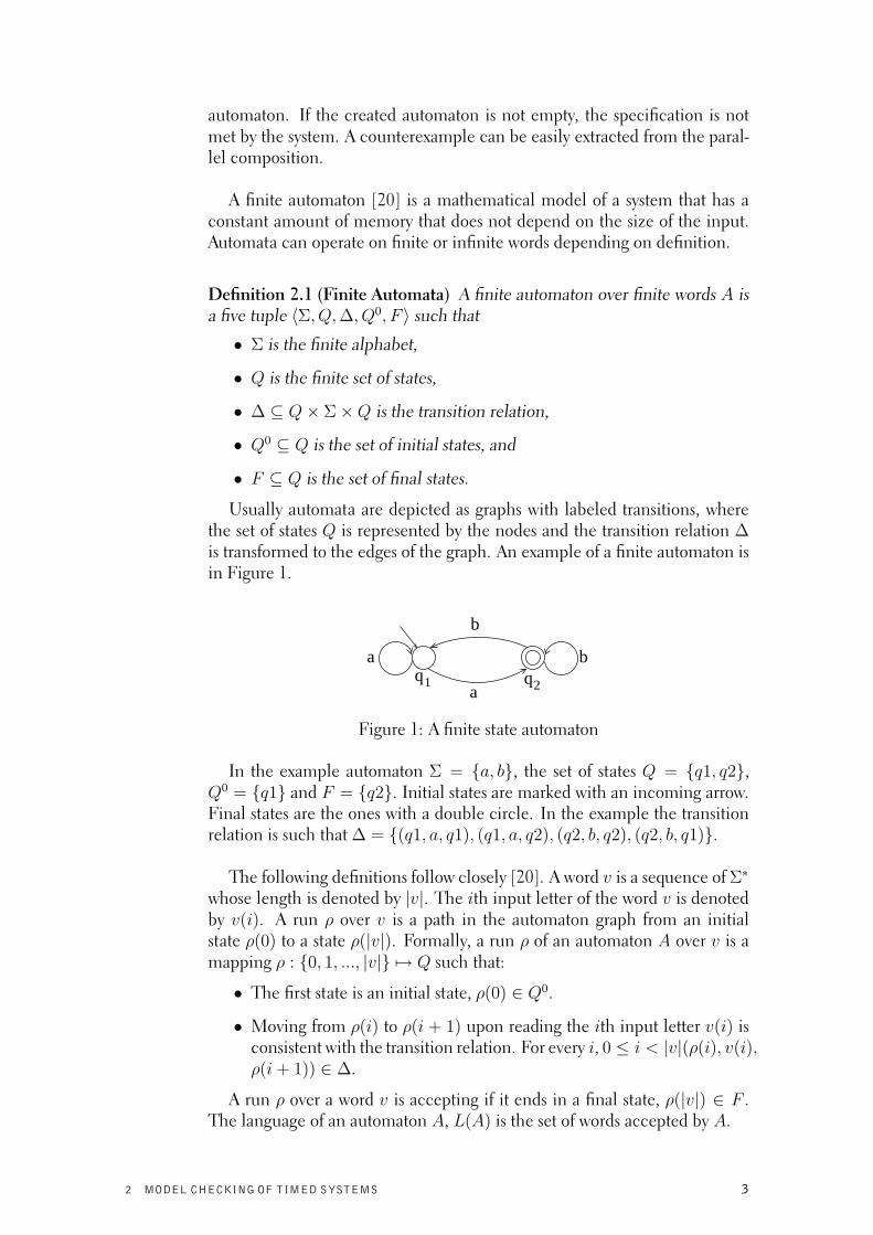
Usually automata are depicted as graphs with labeled transitions, wherethe set of states Q is represented by the nodes and the transition relation ∆is transformed to the edges of the graph. An example of a finite automaton isin Figure 1.

1q q2

b

a

a b

Figure 1: A finite state automaton

In the example automaton Σ = {a, b}, the set of states Q = {q1, q2},Q0 = {q1} and F = {q2}. Initial states are marked with an incoming arrow.Final states are the ones with a double circle. In the example the transitionrelation is such that ∆ = {(q1, a, q1), (q1, a, q2), (q2, b, q2), (q2, b, q1)}.

The following definitions follow closely [20]. A word v is a sequence of Σ∗

whose length is denoted by |v|. The ith input letter of the word v is denotedby v(i). A run ρ over v is a path in the automaton graph from an initialstate ρ(0) to a state ρ(|v|). Formally, a run ρ of an automaton A over v is amapping ρ : {0, 1, ..., |v|} 7→ Q such that:

• The first state is an initial state, ρ(0) ∈ Q0.

• Moving from ρ(i) to ρ(i + 1) upon reading the ith input letter v(i) isconsistent with the transition relation. For every i, 0 ≤ i < |v|(ρ(i), v(i),ρ(i + 1)) ∈ ∆.

A run ρ over a word v is accepting if it ends in a final state, ρ(|v|) ∈ F .The language of an automaton A, L(A) is the set of words accepted by A.

2 MODEL CHECKING OF TIMED SYSTEMS 3

2.1 Timed Automata

Timed automata [3, 8] are used in the model checking of real time systems.Alternative methods with the same goal are e.g., Petri Nets, timed process al-gebras, and real time logics [16, 40, 42, 50]. Timed automata are especiallyneeded when the correct functioning depends fundamentally upon real timeconsiderations. Such a situation is typical when the system must interact witha physical process.

Modal logic [21] considers only the ordering of sequential events, i.e., itabstracts away from time. However, in the linear time model an executionof a system can be modelled as a timed trace, in which the events and theiractual time points are denoted. The behaviour of a system is a set of thesetimed traces. A set of timed traces can be thought of as a set of sequencesthat form a language. If the language is regular, it is possible to use finiteautomata in the process of specification and verification of the system.

In the original theory [3] timed automata are essentially finite state au-tomata extended with real valued clock variables and infinite input. Thefunctionality of the automaton can be restricted by the conditions set to theclocks.

A timed automaton is an abstraction of a real time system. It is basically afinite state automaton with a set of clock variables. The variables model thelogical clocks of the system, and they are initialized with zero when the sys-tem is started. After this, all the clock variables are increased at the same rate.In addition to the clocks, a timed automaton also has guard constraints on itstransitions. A transition can be taken, when the guard constraint on the edgeof the automaton evaluates to true. These guards restrict the behaviour of theautomaton by constraining the values of the clocks allowed for the transitionto be enabled.

Finally, the clock variables can also be reset. This can only happen when atransition is taken. Multiple clocks can be reset at once. The clock variablesare reset after the guard constraint has been evaluated as true.

The problem with the original timed automaton is that the guards onlyenable the transitions. The automaton can not be forced to make transitions.This leads to a possible situation where the automaton stays forever in somestate [8].

A simplified version of a timed automaton, a timed safety automaton [29]is a timed automaton with local state invariants. A timed safety automatonmay stay in a node only as long as the clocks satisfy the invariant of the node.These invariant conditions can eliminate the problem because they can forcethe automaton to make a transition. Because of its simple structure, thetimed safety automaton has been adopted in many timed automata verifica-tion tools including Uppaal [34] and Kronos [51].


WorkStart

x== 5, a, x:= 0

x == 10, c

x >= 20, b, x := 0

Figure 2: A timed automaton

An example of a timed automaton is in Figure 2. The timed automatonin Figure 2 has two locations: Start and Work , and a clock variable x. Start

has a double circle surrounding it indicating the initial location insted of theincoming arrow in Figure 1. The automaton has three transitions. Eachtransition has a guard and an action. There is a transition from Start to itself.The guard of this transition states that the transition can only be taken, whenthe clock variable has value 5 (x == 5). The action related to this transitionis a. The clock is reset after the transition (x := 0). The transition fromStart to Work has a guard x == 10 and an action c. This transition doesnot reset the clock variable. The third transition from Work to Start has aguard x >= 20 and an action b. The guard states that the transition can notbe taken unless x is at least 20. The transition also resets the clock x. It isalso possible to remain in either one of the locations forever. The automatonhas no location invariants.

When location invariants are added to the example automaton, the resultis a timed safety automaton (Figure 3). It has an invariant in both locations.The invariants specify a local condition that Start must be left before x be-comes greater than 10, and Work must be left before x becomes greater than50.

WorkStart

x== 5, a, x:= 0

x == 10, c

x >= 20, b, x := 0x <= 50x <= 10

Figure 3: A timed automaton with invariant constraints

This work concentrates on timed safety automata, and will herefrom referto them as timed automata or automata.

2.1.1 Formal Semantics

Basic definitions of the syntax and semantics of timed automata are given.The definitions follow the semantics in [8]. The following notations are used:N is the set of natural numbers, C is the set of clocks, B(C) is a set of simpleconjunctions of the form x ⊲⊳ c or x − y ⊲⊳ c, where x, y ∈ C, c ∈ N and⊲⊳∈ {<,≤, =,≥, >}. A timed automaton is a finite graph, with transitionslabelled with conditions over and resets of non-negative real valued clockvariables.


Definition 2.2 (Timed Automata) A timed automaton A is defined as a tu-ple 〈L, l0, C, Σ, E, I〉, where

• L is a finite set of locations (or nodes),

• l0 ∈ L is the initial location,

• C is the finite set of clocks,

• Σ is the finite set of actions,

• E ⊆ L×Σ×B(C)×2C ×L is the finite set of edges between locationswith an action, a guard, and a set of clocks to be reset; and

• I : L −→ B(C) assigns invariants to locations.

Next the semantics of a timed automaton is defined. A clock valuation is afunction u : C → R+ from the set of clocks to the non-negative reals. Let R

C

be the set of clock valuations. Let u0(x) = 0 for all x ∈ C. In our notationguards and invariants can be considered as sets of clock valuations. u ∈ I(l)means that the clock valuation u satisfies all the constraints in I(l).

For d ∈ R+, let u + d denote the clock assignment that maps all x ∈ C tou(x)+ d, and for r ⊆ C, let [r 7→ 0]u denote the clock assignment that mapsall clocks in r to 0 and agree with u for the other clocks in C \ r.

The semantics of a timed automaton is defined as a labelled transitionsystem where a state consists of the current location, and the current valuesof the clock variables. Thus, there are two types of transitions between states.

In a delay transition the automaton delays for some time (denotedd→, where

d is a non-negative real). In an action transition an enabled edge is followed

(denoteda→, where a is an action). Consecutive delay-action transitions can

be denoted asd→

a→.

Definition 2.3 (Semantics of Timed Automata) Let (L, l0, C, Σ, E, I) be atimed automaton. The semantics is defined as a labelled transition system〈S, s0,→〉, where S ⊆ L × R

C is the set of states, s0 = (l0, u0) is the initialstate, and →⊆ S × {R+ ∪ Σ} × S is the transition relation such that:

• (l, u)d→ (l, u + d) if ∀d′ : 0 ≤ d′ ≤ d =⇒ u + d′ ∈ I(l), and

• (l, u)a→ (l′, u′) if there exists e = (l, a, g, r, l′) ∈ E such that u ∈

g, u′ = [r 7→ 0]u, and u′ ∈ I(l).

The transition relation is intuitively such that it allows two kind of tran-sitions. Either all the clock values of the automata are increased by somepositive value, or time does not advance at all while an edge of the automa-ton is taken. In the first case the transition must be allowed by the locationinvariants. In the second case the transition can only be taken if the guards


evaluate to true, and the invariant constraints are not violated after the tran-sition’s reset phase. As an example of the semantics, the timed automata inFigure 3 could have the following reachable states:

(Start, x = 0)5→ (Start, x = 5)

a→ (Start, x = 0)

10→ (Start, x =

10)c→ (Work, x = 10)

38→ (Work, x = 48)

b→ (Start, x = 0)...

2.1.2 Decision Problems in Timed Automata

In model checking, we need to be able to ask questions about the function-ing of the automaton used as a model. Operational semantics is the basisfor verification of timed automata [8]. An important question to ask abouta timed automaton is the reachability of a certain state in the automaton.These kind of questions are used to formalize safety properties of the system.It is also important to know how to compare the functioning of two indepen-dent automata. Two main indications of similarity are language inclusionand bisimilarity. Language inclusion means that the set of traces producedby an automaton A is a subset of the set of traces produced by a differentautomaton B. Bisimilarity is a stronger measure of similarity than languageinclusion. A formal definition of bisimulation is presented in what follows.Next, some definitions for language inclusion, bisimulation and reachabilityin timed automata are given. The definitions in [8] are closely followed.

A timed action (t, a) is a pair, where a ∈ Σ is an action performed bythe automaton A at time point t ∈ R+. The absolute time t is called thetime-stamp of the action a. A timed trace ξ = (t1, a1)(t2, a2)(t3, a3)... is asequence of timed actions where ti ≤ ti+1 for all i ≥ 1.

Definition 2.4 A Run of a Timed Automaton A = 〈L, l0, C, Σ, E, I〉 withinitial state 〈l0, u0〉 over a timed trace ξ = (t1, a1)(t2, a2)(t3, a3)... is a se-

quence of transitions: 〈l0, u0〉d1→

a1→ 〈l1, u1〉d2→

a2→ 〈l2, u2〉 · · · satisfying thecondition ti = ti−1 + di for all i ≥ 1.The timed language L(A) is the set of all timed traces ξ for which there existsa run of A over ξ.

Language inclusion problem is undecidable for timed automata [3]. Thisis because timed automata are not determinizable in general. If the timestamps of the traces are not taken into consideration, we can define the un-timed language Luntimed(A) as the set of all traces in the form: a1a2a3... forwhich there exists a timed trace ξ = (t1, a1)(t2, a2)(t3, a3)... ∈ A. The lan-guage inclusion problem for these untimed languages is decidable [3].

It has been shown that timed bisimulation is decidable [15]. Timed bisim-ulation is introduced for timed process algebras in [50], and can be extendedto timed automata [8].

Definition 2.5 (Bisimulation of Timed Automata) A bisimulation R overthe states of timed automata A1 = 〈L1, l10, C

1, Σ, E1, I1〉 and A2 = 〈L2, l20, C2,


Σ, E2, I2〉 is a symmetrical binary relation satisfying the following condition:

for all (s1, s2) ∈ R,

if s1σ→ s′1 ∈ E1 for some σ ∈ Σ and s1, s

′

1 ∈ L1, then s2σ→ s′2 ∈ E2 and

(s′1, s′

2) ∈ R for some s2, s′

2 ∈ L2.

if s2σ→ s′2 ∈ E2 for some σ ∈ Σ and s2, s

′

2 ∈ L2, then s1σ→ s′1 ∈ E1 and

(s′1, s′

2) ∈ R for some s1, s′

1 ∈ L1.

Two automata are timed bisimilar iff there is a bisimulation containingthe initial states of the automata.

In the case of bisimulation, an untimed version is also decidable [35]. We

just consider a timed transition s1d→ s2 as an empty transition s1

ε→ s2. The

alphabet of the automaton is the replaced with Σ ∪ {ε}.

Definition 2.6 (Reachability Analysis of Timed Automata)

Let 〈l, u〉 → 〈l′, u′〉 if 〈l, u〉σ→ 〈l′, u′〉 for some σ ∈ Σ ∪ R+. Let →∗ de-

note n consecutive transitions, where n ∈ N. For an automaton with initialstate 〈l0, u0〉, 〈l, u〉 is reachable iff 〈l0, u0〉 →

∗ 〈l, u〉. More generally, given aconstraint φ ∈ B(C) we say that the configuration 〈l, φ〉 is reachable if 〈l, u〉is reachable for some u satisfying φ.

Reachability analysis offers a lot of model checking properties. Negationsof reachability properties can be used to express invariant properties. Forexample, a system is always in a safe state if the failure states of the system arenot reachable. In addition, reachability analysis of timed automata offers away to examine bounded liveness properties. These properties state that somestate will be reached within a given time. The property can be transformedinto an invariant property using an additional automaton.

2.1.3 Parallel Composition of Timed AutomataA parallel composition of timed automata [3] is an operation used to describecomplex systems using simpler subsystems. A parallel composition describesthe joint functioning of several automata concurrently.

In an untimed version of the parallel composition, it can be defined usingthe traces of the automata. An untimed automaton is totally determined bythe set of its traces. A parallel composition of these trace sets is the set oftraces such that for each automaton the relevant projection is possible in theautomaton. If the event sets of the automata are distinct, the parallel com-position is just the union of the trace sets. If the event sets of the automataare identical, the parallel composition is the set theoretic intersection of thetrace sets.

Next, the parallel composition of timed automata is defined. The def-initions in [3] are closely followed. The projection of an untimed traceξ = a1a2a3... onto an automaton Ai, written ξ⌈Ai is formed by taking only


the events of the trace ξ that are in the event set of the automaton Ai. Theprojection is only considered when the intersection ξ ∩Ai is nonempty. Theparallel composition ‖iAi for a set of untimed automata Ai is thus an un-timed automaton with the event set of ∪iAi. The trace set of the parallelcomposition is the set of traces that exist in at least one of the componentautomata, and can be projected to all of the component automata.

The parallel composition operator can be extended to timed automata aswell. The projection operator is changed so that in the parallel compositionof two processes the common events should always happen at the same time.A composition of two traces with common events will always result in eitheran empty set or a single trace.If, for example, automaton A1 with an event set {a, b} has only a single trace

ξ1 = (a, 1)(b, 2)(a, 4)(b, 5)(a, 7)(b, 8)...

and an automaton A2 with an event set {a, c} has three possible traces:

ξ2 = (a, 1)(a, 4)(a, 7)...ξ3 = (a, 1)(a, 2)(a, 3)...ξ4 = (c, 3)(c, 6)(c, 9)...

The resulting parallel composition A1‖A2 would have an event set of{a, b, c} and a set of traces:

ξC1 = (a, 1)(b, 2)(a, 4)(b, 5)(a, 7)(b, 8)...ξC2 = (a, 1)(b, 2)(c, 3)(a, 4)(b, 5)(c, 6)(a, 7)(b, 8)...

These are the compositions of trace pairs (ξ1, ξ2) and (ξ1, ξ4). The tracepair (ξ1, ξ3) results in an empty trace because the common event a takesplace at different time stamps in the traces.

Following the definitions in [20], the actual timed automaton that repre-sents the parallel composition of two automata A1 = 〈L1, l

10, C1, Σ1, E1, I1〉

and A2 = 〈L2, l20, C2, Σ2, E2, I2〉 is the timed automaton:

A1‖A2 = 〈L1 × L2, l10 × l20, C1 ∪ C2, Σ1 ∪ Σ2, E, I〉

where I(s1, s2) = I1(s1) ∧ I2(s2) and the transition relation E is given bythe following rules:

• For a ∈ Σ1 ∪ Σ2, if 〈s1, a, φ1, λ1, s′

1〉 ∈ E1 and 〈s2, a, φ2, λ2, s′

2〉 ∈ E2,then E will contain the transition 〈(s1, s2), a, φ1∧φ2, λ1∪λ2, (s

′

1, s′

2)〉.

• For a ∈ Σ1 −Σ2 if 〈s, a, φ, λ, s′〉 ∈ E1 and t ∈ L2, then E will containthe transition 〈(s, t), a, φ, λ, (s′, t)〉.

• For a ∈ Σ2 −Σ1 if 〈s, a, φ, λ, s′〉 ∈ E2 and t ∈ L1, then E will containthe transition 〈(t, s), a, φ, λ, (t, s′)〉.


The locations of the parallel composition automaton are pairs of locationsfrom the component automata. Invariants are conjunctions of the invariantsin the component automata. For each pair of transitions from the componentautomata with the same action, there will be a transition in the composite au-tomaton. The transition source state is a pair in the composition that consistsof the source states of the individual automata. The transition target loca-tion is such a pair that is formed from the target locations of the individualtransitions. If an action only exists in one of the automata, the compositiontransition will be such that the other automaton remains unchanged. Such atransition is created for each location of the other automaton.

2.1.4 Symbolic Semantics, Regions and Zones

A timed automaton with real-valued clocks leads to an infinite transition sys-tem. In order to perform efficient verification of timed automata, a finitetransition system must be acquired. The basis of decidability results in timedautomata comes from the concept of region equivalence over clock assign-ments [3]. The next section follows closely the definitions in [8].

Definition 2.7 (Region Equivalence) Let k be a function, called a clockceiling, mapping each clock x ∈ C to a natural number k(x) (i.e. the ceilingof x). For a real number d, let {d} denote the fractional part of d, and let ⌊d⌋denote its integer part. Two clock assignments u, v are region-equivalent, de-noted u

.∼k v, iff

• for all x, either ⌊u(x)⌋ = ⌊v(x)⌋ or both u(x) > k(x) and v(x) > k(x),

• for all x, if u(x) ≤ k(x) then {u(x)} = 0 iff {v(x)} = 0 ; and

• for all x, y if u(x) ≤ k(x) and u(y) ≤ k(y) then {u(x)} ≤ {u(y)} iff{v(x)} ≤ {v(y)}.

A region is an equivalence class denoted [u] that is the set of region-equivalent clock assignments with u. Using the region construction, a finitepartitioning of the state space is possible. This is because each clock has amaximal constant value k(x) which makes the number of regions finite. Theconstant value k(x) is the highest value, against which the clock is compared.

Also, u.∼ v implies that the states of the timed automaton (l, u) and (l, v)

are bisimilar with regard to the untimed bisimulation for any location l ∈ L.The equivalence classes can be used to create a finite-state region automaton.Using a region automaton, many of the decision problems of timed automatabecome decidable. The transition relation between symbolic states of a re-gion automaton is the following:

• 〈l, [u]〉 ⇒ 〈l, [v]〉 if 〈l, u〉d→ 〈l, v〉 for a positive real number d, and

• 〈l, [u]〉 ⇒ 〈l′, [v]〉 if 〈l, u〉a→ 〈l′, v〉 for an action a.


x

y

1 2 3

1

2

Figure 4: Regions of a system

An example of the regions of an automaton with two clocks x and y isin Figure 4. The maximal comparison constants of x and y are 3 and 2,respectively. The example has 60 different time regions. All open areas,lines and intersections count as a region. Possible regions of the exampleare (x = 1, y = 1) (a corner point), (x = 2, y < 1) (a line segment),{(1 < x < 2) ∧ (y < x)} (an open area).

The intuitive idea of using regions is the following: if two states, whichcorrespond to the same location of a timed automaton, have clock valueswith the same integral parts and the ordering of the fractional parts, the twostates will behave similarly.

The problem of the region automata is the exponential growth in the num-ber of regions as the number of clocks or the maximal constants increase.Clock zones [1] can represent the state space of a timed automaton moreefficiently. [19, 29]

The idea of clock zones is that most of the time regions are not needed,and some of them can be united. A clock zone is a set of clock assignmentsi.e. a conjunction of inequalities or a convex union of clock regions, thatcompare a clock value or the difference between two clock values against aninteger. The following types of inequalities are allowed:

x < c, x ≤ c, c < x, c ≤ x, x − y < c, x − y ≤ c

where c is an integer, x, y are clocks. For a clock zone φ, the set of clockvalues satisfying φ will also be denoted φ. If an automaton A has k clocks,then a clock zone φ expressed in terms of these clocks is a convex subset ink-dimensional Euclidean space [20].

For example, one possible zone graph of the timed automaton in Figure 3is in Figure 5.


Start, 0 <= x <= 10

Start, x = 5 Start, x = 10

Work, 10 <= x <= 50

Work, 20 <= x <= 50

Figure 5: The zone graph of the timed automaton in Figure 3

2.1.5 Difference Bound Matrices

Difference bound matrix (DBM) [19] is a way to represent a clock zone ina compact form. We define a difference bound matrix following the defini-tion in [20]. Its definition requires the use of a special clock c0 that alwayshas value 0. The difference bounded matrix is indexed by the set of clocksC0 = C ∪ {c0}. The special clock c0 has the index 0. The entries of the ma-trix Di,j have the form (di,j,≺i,j) that expresses a comparison of two clockvalues ci and cj with an integer di,j. The comparison operator ≺i,j is either <or ≤. The matrix entries represent inequalities ci − cj ≺ di,j, where di,j is ei-ther integer or ∞. The special clock c0 can be used to represent inequalitiesthat only concern one clock variable. As an example, consider the followingclock zone:

c2 − c1 < −2 ∧ c2 ≤ 1 ∧ c1 ≤ 3

The difference bounded matrix is:

D =

(0,≤) (0,≤) (0,≤)(3,≤) (0,≤) (∞, <)(1,≤) (−2, <) (0,≤)

A zone can be represented by | C0 |2 atomic constraints of the formc1 − c2 ≺ n. Each pair is used only once. In the case of two constraintson the same pair of variables, the intersection of these constraints is mean-


ingful. These zones can be stored in | C0 | × | C0 | sized matrices calleddifference bound matrices.

The zone representation is not unique. The same zone can be representedby several different matrices. In our example c1 − c0 ≤ 3 and c0 − c2 ≤ 0implies c1 − c2 ≤ 3. We can change D1,2 to (3,≤) and obtain an alternativeDBM. Generally, the sum of the upper bounds ci − cj and cj − ck is an up-per bound on the clock difference ci − ck. Reducing the clock differences totighten the difference bound matrix is done as follows:

If ci − cj ≺i,j di,j and cj − ck ≺j,k dj,k, then ci − ck ≺′

i,k d′

i,k whered′

i,k = di,j + dj,k and

≺′

i,k=

{

≤ if ≺i,j=≤ and ≺j,k=≤< otherwise

If (d′

i,k,≺′

i,k) is a tighter bound than (di,k,≺i,k), the original bound canbe replaced by the new one. The operation is called tightening. The DBMis in a canonical form when no further tightening is possible. The canonicalform of the DBM in our example is:

D =

(0,≤) (−2, <) (1, <)(3,≤) (0,≤) (3,≤)(1, <) (−2, <) (0,≤)

2.2 Temporal Logic with Real Time

Temporal logic is an extension of classical logic that can be used to create for-mal system specifications. These formal specifications can then be checkedusing some model checking method. With temporal logic unambiguous de-scriptions such as "The system never reaches an erroneous state." or "Thisaction always leads to the resetting of the system." can be written.

Temporal logics can be classified according to the assumed structure oftime. Some temporal logics assume linear time structure, some assume abranching time structure. Computation tree logic (CTL) [20] is a branchingtime logic. It is used when the models that are verified are finite state systemsthat abstract away from time. It is assumed that an execution can be mod-elled as a linear sequence of system events.

Timed computation tree logic (TCTL) [2] is an extension of CTL to realtime systems. For real time systems ordinary CTL is not sufficient, since a sys-tem’s correctness depends on the values of the timing delays. Sometimes it isnot enough if a function is known to eventually happen. In real time systemswe need to know whether the action takes place within a certain time period.

In order to create real time models and specifications, using event se-quences is not sufficient and therefore timed traces are needed. Timed traces


associate with each state the time of the occurrence of the event. The conceptof time can be modelled in different ways. In the case of timed computationtree logic a dense-time model is preferred. In a dense-time model the timesof events are real numbers, that increase monotonically without a bound [3].TCTL was created to describe CTL specifications in real time.

In TCTL, quantitative temporal operators are introduced to describe timedproperties. First, the syntax and semantics of the branching-time logic CTLare reviewed. Next, the TCTL extensions to the CTL syntax are defined.TCTL semantics is also represented.

2.2.1 Computation Tree LogicIn CTL time is seen as a tree-like structure in which the future in not de-termined. Different possible futures exist, and any of these is possible. Thefollowing section follows the notations in [20].

CTL formulas consist of logical operators, path quantifiers and temporaloperators. Path quantifiers (A(”for all computation paths”) and E(”for somecomputation path”)) are used in a state to specify that all of the paths (A)or some of the paths (E) starting from that state have some property. Thetemporal operators describe properties of a path of the tree. Several temporaloperators exist. Here, only some are defined, since others can be definedusing them.

• X ("next") requires that the property holds at the next state of the path.

• U ("until") is a binary operator. Formula P U Q holds when P is trueuntil Q becomes true. Also, the second argument must become true atsome point.

Given a finite set of atomic propositions {AP}, the CTL formulas can beinductively defined as follows:

φ ::= p | false | φ1 → φ2 |

| EXφ1 | E [φ1U φ2] | A [φ1U φ2]

where p ∈ AP is an atomic proposition and φ1, φ2 are CTL formulas. EXφ1

means that there is an immediate successor state that is reachable in onestep, in which φ1 is true. E [φ1U φ2] requires that there is a path in which φ2

becomes true at some time point t. Also, φ1 must be true on that path untilt. A [φ1U φ2] means that for every computation path, the previous conditionholds.

Other often used temporal operators are for example: EFφ for E [trueU φ],AFφ for A [trueU φ], EGφ for ¬AF¬φ and AGφ for ¬EF¬φ.

The semantics of CTL is defined with respect to a Kripke structure M =〈S, R, L〉, where S is the set of states, R ⊆ S × S is the total transition rela-tion, and L : S → 2AP is the labelling function. A path in M is an infinite


sequence of states, π = s0, s1, s2, ... such that for every i ≥ 0, (si, si+1) ∈ R.We denote with πi the suffix of π starting at si. Notation M, s |= f means thatf holds at a state s in a structure M . Let Tr(s) = {π = s0, s1, ... | s0 = s}be the set of possible paths starting from the state s. The satisfaction relation|= is defined inductively:

M, s |= p iff p ∈ L(s)

M, s |= ¬φ iff M, s 2 φ

M, s |= φ1 → φ2 iff M, s 2 φ1 or M, s |= φ2

M, s |= EXφ iff ∃s1 ∈ S, s.t. ,(s, s1) ∈ R and M, s1 |= φ

M, s |= A[φ1Uφ2] iff ∀π = s0, s1, s2... ∈ Tr(s) :

∃i((M, si |= φ2) ∧ (∀(j < i)M, sj |= φ1))

M, s |= E[φ1Uφ2] iff ∃π = s0, s1, s2... ∈ Tr(s) :

∃i((M, si |= φ2) ∧ (∀(j < i)M, sj |= φ1))

2.2.2 Timed Computation Tree Logic

It is possible to write properties like EFp in CTL. However, CTL does notprovide a way to bound the time at which p happens. TCTL extends the tem-poral operators so that it is possible to limit their scope in time. It is possibleto write for example EF<5p meaning that at some computation path p willbecome true within 5 time units. TCTL syntax is shortly:

φ ::= p | false | φ1 → φ2 |

| E [φ1U∼c φ2] | A [φ1U∼c φ2]

where p ∈ AP is an atomic proposition, c ∈ N , φ1 and φ2 are TCTL formu-las and ∼∈ {<,≤, =,≥, >}.

E [φ1U<c φ2] means that for some computation path there exists a prefixof time length less than c time steps, such that at the last state of the pre-fix φ2 holds, and φ1 is true in all the states in the path until the last state.A [φ1U<c φ2] means that the above condition holds on every computationpath. It is also possible to create TCTL formulas for time intervals. For ex-ample a formula EF(a,b)φ meaning "φ holds at least once between time stepsa and b" can be written EF=aEF<(b−a)φ.

Since TCTL operates in a dense time domain and not in a discrete timedomain like CTL, the next-time operator can not be used. By definition,there is no unique next time point. The computation paths in TCTL withdense time domain are maps from the real valued time domain R to statesof the system. There is a unique state at every real valued time instant. For aset of states S and a state s ∈ S an s-path through S is a map p from R to Ssatisfying p(0) = s. The computation tree in dense time is a map from every


state to a set of paths starting at that state. The prefix of an s-path up to timet is denoted pt. The concatenation of two s-paths p1 and p2 is denoted p1 �p2.

The structure that TCTL can be defined against can not be exactly thesame as in the of CTL. The TCTL structure is a triple M = 〈S, f, L〉 whereS is the set of states, L : S → 2AP is the labelling function, and f is a mapgiving for each s ∈ S a set of s-paths through S. f satisfies the tree constraint:

∀s ∈ S.∀p ∈ f(s).∀t ∈ R.pt � f [p(t)] ⊆ f(s).

The satisfaction relation |= for TCTL is defined inductively:

M, s |= p iff p ∈ L(s)

M, s |= ¬φ iff M, s 2 φ

M, s |= φ1 → φ2 iff M, s 2 φ1 or M, s |= φ2

M, s |= A[φ1U∼cφ2] iff ∀p ∈ f(s) : ∃t ∼ c, p(t) |= φ2 ∧

(∀(0 < t′ < t)p(t′) |= φ1)

M, s |= E[φ1U∼cφ2] iff ∃p ∈ f(s) : ∃t ∼ c, p(t) |= φ2 ∧

(∀(0 < t′ < t)p(t′) |= φ1)

2.3 Model Checking Tool Uppaal

Uppaal is a tool for model checking of timed systems. Other tools for mod-elling and verification based on timed automata are e.g., Kronos [51] andRED [48].

The Uppaal modelling language [34] is based on networks of timed au-tomata. A network of timed automata is a parallel composition A1 | · · · | An

of timed automata A1, ...An, referred to as processes. The definition of aparallel composition varies depending on the used process calculi. In Up-paal the parallel composition operator of Calculus of Communicating Sys-tems (CCS) [39] is used. Hand-shake synchronization with input and outputactions is used for synchronous communication. Asynchronous communi-cation happens through shared variables. For hand-shake synchronizationpurposes the action alphabet Σ in Uppaal consist of symbols a? for input ac-tions and a! for output actions. Internal actions are represented by a distinctsymbol τ . Next we define a network of timed automata formally.

A network of timed automata has a common set of clocks and actions. Thenetwork consists of n timed automata Ai = (Li, l

0i , C, Σ, Ei, Ii), 1 ≤ i ≤ n.

A location vector is l = (l1, ..., ln). We write I(l) =∧

i Ii(li) as a compositionof the invariant functions. Let l[l′i/li] mark the vector l with the ith elementli replaced by l′i.

Definition 2.8 (Semantics of a network Timed Automata) Let Ai =(Li, l

0i , C, Σ, Ei, Ii), 1 ≤ i ≤ n. be a network of timed automata. Let l0 =


(l01, ..., l0n) be the initial location vector. The semantics is defined as a labelled

transition system 〈S, s0,→〉, where S = (L1 × · · · × Ln) × RC is the set of

states, s0 = (l0, u0) is the initial state, and →⊆ S × {R+ ∪ Σ} × S is thetransition relation defined by:

• (l, u) → (l, u + d) if ∀d′ : 0 ≤ d′ ≤ d =⇒ u + d′ ∈ I(l)

• (l, u) → (l[l′i/li], u′) if there exists li

agr−→ l′i such that u ∈ g, u′ = [r 7→

0]u, and u′ ∈ I(l) ; and

• (l, u) → (l[l′j/lj, l′

i/li], u′) if there exists li

c?giri−→ l′i and lj

c!gjrj

−→ l′j such

that u ∈ (gi ∧ gj), u′ = [ri ∪ rj 7→ 0]u and u′ ∈ I(l).

2.3.1 Modelling in UppaalModelling in Uppaal is done via a graphical user interface. Timed automa-ton templates can be created with the Uppaal modelling tool. Every templatehas its own local declaration section, where local variables and functions canbe introduced. There is also a global declarations’ section for global variablesand functions. Finally, a section for process declaration is needed. In thispart the automaton instances are created from the templates, and the paral-lel composition of these is declared for property checking and simulation.

In addition to creating networks of timed automata, the Uppaal modellinglanguage is extended with several modelling features:

• Templates of automata can be defined with a set of parameters. Theparameters are substituted in the process declaration part.

• Integer constants can be defined.

• Bounded integer variables (int[min, max]) can be defined.

• Binary synchronization channels can be declared.

• Broadcast channels can be declared. In broadcast synchronization onetransition labelled with an output action can synchronize with severaltransitions labelled with an input action.

• Synchronization channels can be declared urgent by prefixing the chan-nel declaration with the keyword urgent. When a transition labelledwith an urgent synchronization is enabled (i.e., it can be taken), timeis not allowed to pass. However, the synchronization transition neednot be taken if other transitions are possible.

• Locations can be declared urgent. When a system is in an urgent loca-tion, no time is allowed to pass.

• Locations can be declared committed. A state is committed if oneor more locations in the state are committed. When a system state iscommitted, no time is allowed to pass. Also, the next transition must besuch that an outgoing edge of at least one of the committed locationsis involved.


• Arrays of clocks, channels, constants or integers can be declared.

• Integer variables and arrays can be initialized.

2.3.2 Verification in Uppaal

As specifications, Uppaal accepts a subset of TCTL formulas. In general,Uppaal does not allow nesting of temporal operators, or bounded specifica-tions. In Uppaal syntax [] is equivalent to the TCTL G, or "globally". 〈〉 isequivalent to the TCTL F, or "finally". The notation p − − > q (p leads toq) is an abbreviation of A[](p imply A <> q).

In Uppaal specifications, the dot character (.) is used to reference the vari-ables and states of a particular timed automaton. For example A.l referencesto the location or variable l of automaton A.

In the verification process, Uppaal uses symbolic states of the timed au-tomata 〈l, D〉 where l is a location of the automaton, and D is a zone storedin memory as a DBM [5]. The Uppaal tool calculates the parallel composi-tion of the timed automata in the model, and performs reachability analysison the structure in order to verify it against a property. In other words, thetool goes through the state space, and tries to find a state, in which the prop-erty is false.

Not all specifications can be stated in TCTL as supported by Uppaal. Inthese cases some modelling tricks can be used. Often it is possible to cre-ate an additional observer automaton that observes the behaviour of someother automata. For instance, bounded liveness properties of TCTL can bechecked using an observer automaton.

An example of an observer automaton is in Figure 6. Using the observerautomaton, a bounded liveness property:

AG alarm imply AF <50 observation

that can not be checked as such with Uppaal, can be stated differently as:A[℄ not Observer.FailureObserver automata can be used in many ways and with various properties.

FailureDetecttime <= 50

Idle

observation

time == 50 and not observation

alarm?time :=0

Figure 6: An observer automaton in Uppaal


3 TIMED SAFETY INSTRUMENTED SYSTEMS

3.1 Programmable Logic Controller

A programmable logic controller (PLC) defined in IEC 1131-3 is a digitalcomputer that can be used in automation control and safety instrumentationcontrol.

PLCs have evolved from simple logic controllers used to control physicalprocesses that have a number of inputs, outputs, relays and timers. PLCswere designed as a replacement to logic controllers with relays [23]. PLCs,however, can be modified to work like different logic controllers. The IECstandard describes five different programming language standards for PLCs:

• Ladder diagram (LD),

• Function block diagram (FBD),

• Structured text (ST),

• Instruction list (IL), and

• Sequential function chart (SFC).

Structured text and instruction list are textual PLC programming lan-guages. The other three are graphical diagram based languages. PLCs sup-port complex features such as multi-tasking and interrupts, but these are notnecessary, and will only make the verification difficult. Therefore, a simpleversion of a PLC is used throughout this work. The characterization follows.

A PLC program uses two memory areas reserved for input and output sig-nal values. Before each execution cycle the sensors of the PLC are polledand the values are copied to the memory area reserved for the input signals.This part of memory contains the snapshot of the input values at the time ofthe polling. After the PLC program has been executed, the output values areupdated. A well written PLC program terminates within a bounded amountof time which is less than the cycle time of the PLC. The PLC program willinitiate the next cycle after some fixed amount of time.

Timers are pieces of programs used with systems that need real-time fea-tures. The timers used in our simple version of a PLC are of type TON(Timer On Delay). A TON timer has some signal as an input IN , a pre-set integer value PT , an internal accumulator variable, timers base intervalvalue, and two output signals Q and ET . The timer records the number ofbase intervals the input signal has been true, and increases the accumulatorvalue accordingly. When the accumulator value is greater than or equal tothe preset value PT , the output signal Q is turned on. ET is an integer out-put that has an initial value of 0. In every cycle the value of ET is increasedby 1, if the IN is true, and the current value of ET is less than PT . If IN istrue, and ET is not less than PT , the value of ET is not increased. Whenthe input IN is false, both outputs are reset to zero. The preset value PT can

3 TIMED SAFETY INSTRUMENTED SYSTEMS 19

also be seen as an integer input. A TON timer is represented in Figure 7.

TON

Preset value pre

Accumulator acc

Base interval 1.0IN

PT

Q

ET

Figure 7: A TON timer with inputs IN and PT, and outputs Q and ET

The functionality of a TON timer is in Figure 8.

IN

Q

ET

time

PT PT PT

Figure 8: Functionality of a TON timer

3.2 Safety Instrumented Systems

Industrial processes involve great risks because of dangerous temperatures,pressures and materials. Therefore, separate systems to protect environment,personnel and equipment are needed. In the ANSI/ISA-84.00.01-2004 (IEC61511) standard a safety instrumented system (SIS) [23] is defined as an "in-strumented system used to implement one or more safety instrumented func-tions. A SIS is composed of any combination of sensor(s), logic solver(s), andfinal element(s)". The purpose of a SIS is to either automatically take an in-dustrial process to a safe state, when predetermined conditions are violated;allow a process to move forward when the predetermined conditions are true;or mitigate the consequences of an industrial hazard. A SIS is designed to al-ways work in a risk reducing manner. [23]

The sensors of a SIS collect information of the state of the process. Sen-sors can measure temperature, pressure, flow or other process parameters.The logic solver makes decisions of the actions taken based on the sensors’signals. A typical action is a signal sent to the final elements. Final elementsare usually valves or electrical switches that have some risk reducing effect

20 3 TIMED SAFETY INSTRUMENTED SYSTEMS

on the process.

An example of a SIS is an emergency cooling system of a reactor. TheSIS has heat sensors, and a logic, which determines when the safety instru-mented function is initiated. In this case the safety instrumented function isthe opening of a coolant valve. Similarly, a SIS observing the pressure of atank, initiates an open action of a pressure releasing valve.

As mentioned earlier, PLCs can be used as the logic solvers of safety in-strumented systems. Since, PLCs are increasingly used in safety critical sys-tems, testing and verification of PLC applications has become very important[23].

4 MODELLING SYSTEMS WITH TIMED AUTOMATA

In this section, some research in the area of model checking with timed au-tomata is surveyed. The research can be roughly divided into model check-ing of real-time communication protocols, and model checking of real-timecontrollers. Most of the surveyed case studies use the model checking toolUppaal. A comprehensive tutorial on Uppaal is in [6]. In this paper the toolitself and its use is described. In addition, two extensive examples and somemodelling conventions are given.

4.1 Modelling Real-Time Communication Protocols

Protocol verification has been of interest to many research groups. Networkand other communication protocols have been modelled and verified usingUppaal, and other modelling tools. Several protocols that have been com-monly in use have been found erroneous, and corrected using Uppaal.

In [44] and [43] a fault tolerant clock synchronization mechanism for aController Area Network (CAN) was modelled and verified. The modellingwas done using the Uppaal tool. The goal of the work was to formally verifythe precision that could be achieved, and the effects of faults to the preci-sion. In their system, master nodes regularly transfer clock synchronizationmessages to the slave nodes. As an essential part of this research, clock drift-ing was modelled using clock automata where the clocks operated in variablelength cycles. In their model the clock rate could change dynamically. Theclock synchronization system corrected both the offset and the drift error ofthe clocks. A certain precision was verified using an observer automaton thatcompared the clocks of the nodes.

In [7] the correctness of the Philips Audio Control Protocol was verifiedusing the Uppaal tool. The analysis was performed on a system with twosenders. Consequently, the bus collision problem was present. In addi-tion, for an incorrect implementation of the protocol, a counterexample wasfound. An important observation of the paper was the usefulness of the com-

4 MODELLING SYSTEMS WITH TIMED AUTOMATA 21

mitted locations in Uppaal. The Uppaal tool was extended to include thesefeatures. In this research, clocks with drifting timespeeds were used. Thesystem was verified for an error tolerance of 5 % on the timing.

In [33] a Collision Avoidance Protocol was studied. The protocol wasmodelled and verified using two tools SPIN [31] and Uppaal. The timed as-pects were easy to model with Uppaal. It was also noticed that the notion ofcommitted locations in Uppaal supported the modelling of broadcast com-munication, and yielded significant reductions in time- and space-usages.

An Audio/Video protocol by Bang & Olufsen (B&O) was studied in [27].The protocol controls the transmission of messages over a single bus, and de-tects collisions. The protocol was known to be faulty, although the cause ofthe fault could not have been pinpointed before. Using the Uppaal tool, anerror trace was extracted. This led to the detection of the error in the imple-mentation. The corrected implementation was successfully verified.

As a continuation to [27] a different Power Down protocol by Bang &Olufsen was studied in [26]. The modelling of the system resulted in thediscovery of three design errors that were identified and corrected. In thispaper, modelling techniques for time slicing problems with interruptions areintroduced. In addition, three observer automaton techniques for propertyverification are introduced.

A bounded retransmission protocol is studied in [18]. In the paper a filetransfer service is first specified by stating several logical properties. Thebounded retransmission protocol’s conformance to these properties is thenchecked using Uppaal and SPIN. The timed properties are checked usingUppaal.

The Pragmatic General Multicast (PGM) protocol is analyzed in [12].The protocol intends to guarantee a reliability property: "a receiver eitherreceives all data packets from transmissions and repairs or is able to detectunrecoverable data packet loss" A simplified model of the protocol is builtand two reliability properties are checked with Uppaal. The properties wereverified only with some parameter values, which the paper presents.

In [36] a method for modelling and verifying of the LEGO RCX programsis introduced. A tool is developed, which can automatically translate RCXprograms into Uppaal models. Also, a system of two RCX units communicat-ing through an infrared channel is built. In their research their IR protocoland Fischer’s mutual exclusion protocol are verified. Their experiments withan actual system of two communicating RCX units showed that an Uppaalmodel could be created using their tool, but the model could not be verifiedbecause of its complexity.

22 4 MODELLING SYSTEMS WITH TIMED AUTOMATA

4.2 Modelling Real-Time Controllers

Controllers have also been of interest to many researchers. Programmablelogic controllers (PLCs) that are also analyzed in this work are analyzed in[32], [49], [4] and [38].

In [32] software analysis techniques for PLCs are developed. Various ver-ification techniques are considered for two PLC programming languages:instruction list (IL) and sequential function charts (SFCs). In this work a for-mal semantics is created for both languages. A model checking method forthe untimed version of a SFC program is presented. The analysis techniquesare also implemented in industrial size case studies.

In [49] a method is developed to analyze simple PLCs written in the in-struction list (IL) language. The PLCs are converted into timed automatathat can be verified using Uppaal. The simple PLCs discussed in this paperuse the TON timers discussed in Section 3.1.

In [4], PLCs designed graphically using Sequential Function Charts (SFCs)are converted into models that can be analyzed using model checking tech-niques. Two approaches are introduced. Both Cadence SMV and Uppaalare applied.

In [38], two examples of analyzing PLC applications with Uppaal are pre-sented. The PLC timing is modelled in detail. Especially the reaction timeof the PLC to a signal is observed. In the first example the PLC just readsinput and writes output. The second example utilizes a TON timer: thetimer is set when the PLC receives input. PLC output is set when the timer’stimeout is recognized.

A distributed lift system was re-examined in [41]. The lift system was pre-viously found faulty in [25], but the errors were fixed in an ad hoc mannerby the system developers. In this paper the developers’ solutions are analyzedusing Uppaal. The solutions are shown to be incorrect. A different solutionis proposed and proven to be correct.

In [28] it is shown how model checking can be used in the designing pro-cess of a deadlock free wafer scanner controller with an optimized through-put. Deadlock situations are possible, since the wafers are handled by robotsthat work independently. In their work a deadlock avoidance policy is firstanalyzed based on a finite state model using the SMV model checker. Athroughput analysis can then be performed on a more detailed timed au-tomaton model using the Uppaal tool. The two models (the SMV modeland the Uppaal model) are formally related through the notion of a stutteringbisimulation introduced by Browne et al. [14]. In the throughput optimiza-tion part an observer automaton is used to measure the progress of the system.It observes the unload events of wafers that had already been scanned. Theobserver is used to find an infinite schedule that takes at most H time unitsuntil the first unload event, and that has at most S time units between two

4 MODELLING SYSTEMS WITH TIMED AUTOMATA 23

unload events.

In [13] a wafer scanner system is analyzed using model-based techniques.As a part of their analysis the system is modelled with the process algebraiclanguage χ (Chi) [47]. The model is then translated into Uppaal timed au-tomata. Some properties are then verified using the Uppaal model.

In [11] a turntable system is analyzed using various model checking tools.A χ (Chi) [47] simulation model is translated into model written in the in-put languages of CADP [22], SPIN and Uppaal. They concluded that Up-paal is the easiest to translate to. Verification of properties with fairness con-straints [20] can be done in CADP and SPIN but is impossible in Uppaal.

In [37] a prototype gear controller is designed and analyzed. Uppaal isused to verify the design. The paper also introduces a method to verifybounded response time properties in Uppaal without an observer automa-ton. Extra variables (boolean variables and clock variables) are used instead.

4.3 Other Real-Time Research

In [30], techniques for generating timed test cases are introduced. In the pa-per the examined environment and the system under test are both modelledas timed automata. Using the presented techniques, both single purpose,and coverage based test cases are then obtained as counterexamples given byUppaal.

5 CASE STUDY: FALCON

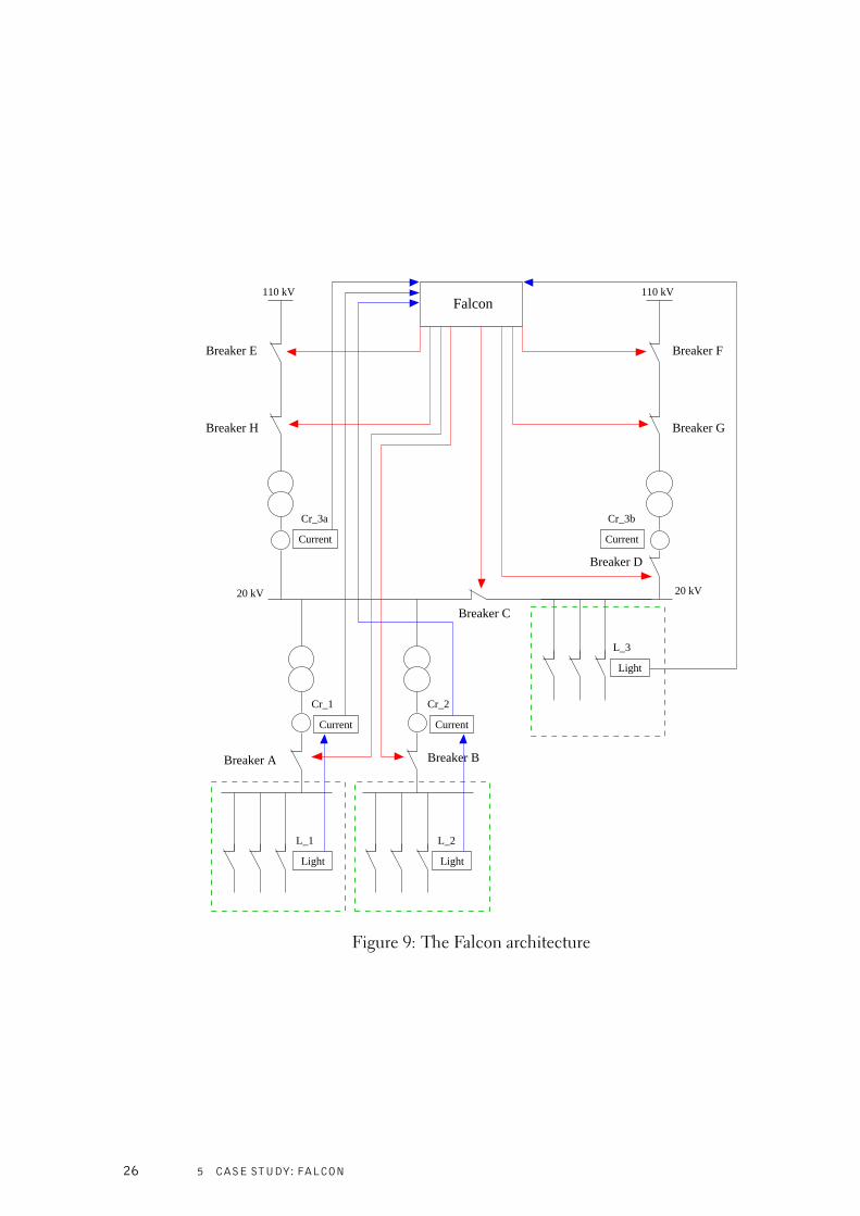
5.1 The Falcon Arc Protection System

The Falcon arc protection system is designed by the engineering companyUrho Tuominen Oy (UTU). The system is designed to increase personnelsafety and minimize material damages in case of an electric arc, e.g., inswitchgear. This is accomplished by cutting off the electricity, when an elec-tric arc is observed. The Falcon system consists of the UTU-Falcon masterunit, several light sensors and several current sensors. The master unit is im-plemented as a programmable logic controller (PLC). It is possible to designnew logical protection architectures that can be uploaded to the master unit.An example of such a logic is in Figure 10.

The devices used to cut electricity are circuit breakers. Circuit breakersare automatically-operated switches that operate in a matter of milliseconds.Their operation is somewhat similar to fuses, but circuit breakers can be reseteither automatically or manually.

The master unit operates in cycles. On each cycle, the master unit readsthe inputs from its sensors and sends output signals according to its pro-

24 5 CASE STUDY: FALCON

grammed logic. Typically the master unit reacts to simultaneous light andcurrent alarms by giving a tripping command to the circuit breakers.

The arc protection system can also be designed to work selectively. Thismeans that electricity is not cut off in every part of the protected area. In-stead, only the affected areas are cut off. If the electrical arc does not disap-pear, an even larger area must be shut down. This kind of selective behaviouris created by placement of the breakers, and the delay components inside theFalcon master unit. The delay components are TON timers introduced inSection 3.1. Intuitively, as soon as an alarm is detected, it is responded to.If the alarm does not disappear, the TON timers in the master unit logic re-ceive continuous input. After some preprogrammed number of cycles, theTON timers give out a signal to some secondary breakers. The secondarybreakers will cut off the electricity more extensively.

5.2 System Environment Description

The environment and architecture used in this case study is identical tothe one used in [45]. The architecture of this case study is made by MattiKoskimies. It is used here with his permission. The architecture is repre-sented in Figure 9.

Electricity is distributed by two distinct power sources. The protected areais divided into three different zones. Each zone has a primary breaker (break-ers A, B, D), that will cut the zone off the power network, if an arc is de-tected. The breaker C is used to separate the power sources. The breakerC is always tripped, when an arc is observed. The secondary breaker G istripped if the alarm has not disappeared after tripping the primary breakerD. The secondary breaker H is tripped if the alarm still has not disappearedafter tripping C, D and G. Similarly, the secondary breaker E is tripped if thealarm has not disappeared after tripping the primary breaker A or B (or both).The secondary breaker F is tripped if the alarm still has not disappeared aftertripping A (or B), C and E. The secondary breakers are not tripped immedi-ately after the primary breakers. Some time must first pass so that the primarybreakers have time to operate.

The Falcon master unit logic that actualizes this behaviour is in Figure 10.The logic consists of seven input signals, AND gates, OR gates, four delaygates, and eight output signals. Four of the input signals (Cr_1, Cr_2, Cr_3a,Cr_3b) are current alarms signals. The remaining three input signals (L_1,L_2, L_3) are the light alarm signals.

The output signals can be divided into two groups. The fast triac outputs(Triac 1, Triac 2, Triac 3, Triac 4) trigger the primary circuit breakers (A, B,C, D). The slower relay outputs (Relay 1, Relay 2, Relay 3, Relay 4) triggerthe secondary circuit breakers (E, F, G, H).

The delay gates are the TON timers introduced in Section 3.1. A signalpasses through a delay gate when the gate receives a preset amount of succes-

5 CASE STUDY: FALCON 25

Current Current

Current Current

Light

Light

Falcon

Light

L_2

Breaker E

Breaker H

Breaker F

Breaker G

Breaker C

Breaker A

Cr_3a Cr_3b

L_1

L_3

Cr_2Cr_1

20 kV20 kV

110 kV 110 kV

Breaker D

Breaker B

Figure 9: The Falcon architecture


sive input signal alarms. The idea is to let the primary breakers try to solvethe problem first. After the preset time limit, the secondary breakers takeaction.

It is important that an arc protection system does not cut the electricity invain. A single current alarm, or a single light alarm typically does not indicatean electric arc. Only in case of both of these alarms concurrently from thesame area should lead to the cutting of the electricity. On the other hand,the arc protection system should always eventually cut the electricity, if theconcurrent current-light alarm does not disappear.

AND

AND

ANDOR

OR

OR

Cr_2L_2

L_1

Cr_1

L_3

Cr_3a

Cr_3b

120

190

60

120

Triac 1

Triac 2

Triac 3

Triac 4

Relay 1

Relay 2

Relay 3

Relay 4

Breaker A

Breaker B

Breaker C

Breaker D

Breaker E

Breaker F

Breaker G

Breaker H

Figure 10: Falcon master unit logic of the example case

5.3 Discrete-time Model

A discrete-time model of the Falcon system can be constructed from threedifferent kinds of automata: the Falcon control unit automaton, primarybreaker automata, and secondary breaker automata. The primary and sec-ondary breakers need distinct automata since their behaviour in the model issomewhat different. Primary breakers can get broken. However, it is assumedthat the secondary breakers are always able to operate. This assumption ismade because we are not really interested in situations where all the breakersinvolved are broken. In these cases it does not really matter how the controlunit reacts to the signals.

Next, the model is explained in more detail. The automata are repre-sented as figures. All the code related to the discrete-time model of theFalcon case is in Appendix A. This includes global declarations, templateinstantiations and the system composition.


5.3.1 The Falcon Control Unit

Idletime<= 1

Cr_1_S: int[0,1], Cr_2_S: int[0,1], Cr_3a_S: int[0,1],Cr_3b_S: int[0,1], L_1_S: int[0,1], L_2_S: int[0,1], L_3_S: int[0,1] time==1

check!getvalues(Cr_1_S, Cr_2_S, Cr_3a_S, Cr_3b_S, L_1_S, L_2_S, L_3_S), time=0

Figure 11: The Falcon system model with discrete time

The timed automaton of the Falcon control unit is in Figure 11. The lo-cal declarations of the automaton are in Appendix A. The automaton hasonly one state, Idle. There is only one transition from that state to itself.In addition, the automaton has seven boolean input variables, seven integervariables for internal calculations, and one clock variable. The automaton isconstructed so that the only transition is taken repeatedly on constant timeintervals, since the real Falcon system operates similarly. This behaviouris forced by an invariant constraint on the clock variable time : time <= 1

and a guard constraint time == 1 in the transition. The combination ofthese constraints forces the automaton to take the transition exactly whentime == 1 . The transition is taken repeatedly because the clock variable isalso reset to zero during the transition.

So far we have accomplished a transition that is taken on constant inter-vals. In addition to the guard constraint, the transition has three other parts:selection, updating and synchronization. All the parts are executed at thesame time point.

The selection part of the transition (Cr_1_S : int[0, 1], Cr_2_S : int [0 , 1 ],Cr_3a_S : int[0, 1], Cr_3b_S : int[0, 1], L_1_S : int[0, 1], L_2_S : int[0, 1],L_3_S : int [0 , 1 ]) introduces seven boolean variables that are given a booleanvalue nondeterministically. These values are later used to determine thevalues of the overcurrent signal inputs Cr_1 ,Cr_2 ,Cr_3a,Cr_3b and thelight signal inputs L_1 ,L_2 ,L_3 . The input values are not given values di-rectly because it might be the case that electricity has already been cut off ina way that some overcurrent signals are impossible. Therefore only interme-diate values for the inputs are chosen. The real input values are then filteredfrom these intermediate values.

The update part of the transition (getvalues(Cr_1_S ,Cr_2_S ,Cr_3a_S ,Cr_3b_S ,L_1_S ,L_2_S ,L_3_S ), time = 0 ) resets the clock and calls thefunctiongetvalues with the selected suggestions for inputs as parameters. The func-tion getvalues is in Appendix A. The objective of this function is to deter-mine the input values, and calculate the outputs using these inputs. First,it is calculated whether electricity is available in the three different zones ofthe system. This information can be concluded because we know whether


each breaker has cut or not. Secondly, the sensors can detect an overcurrentonly if the sensor is connected to the zone it is observing. There is a breakerC between zone 3 and the sensor detecting the value Cr_3a. The breaker Dis between zone 3 and the sensor detecting the value Cr_3b. Using logicalAND, the actual input values are calculated.

Using the inputs and the logic chosen for the system, the fast triac outputsare easy to calculate. The delayed outputs are slightly more complicated.Each of these outputs are associated with a TON timer introduced in Sec-tion 3.1. Three variables are used for every timer-output pair: relayN , rNand relNbuffer , where N ∈ {1, 2, 3, 4} is the number of the output variable.rN is an integer given as a parameter to the Falcon control unit automaton.It determines how many Falcon cycles the boolean variable relayN has to betrue until the information is sent to the breakers. relNbuffer calculates thenumber of consecutive cycles relayN has been true. When the number ofcycles is insufficient the variable relayN is reset to zero. This is done becausethe variable is declared globally. Each secondary breaker observes the valueof one of these variables. If relayN == true is detected by them, it indi-cates that also relNbuffer == rN . The behaviour of the function getvalues

is atomic. Breakers can not detect the temporary relayN == true values ifthe variable is reset later in the function.

Finally, the inputs are reset. This is done to avoid state space explosion. Ifa property that refers to the inputs is checked, it will be necessary to removethe last lines from this function.

The last part of the control unit automaton’s transition is the synchroniza-tion. It is a way of communication in the system. The message (check !) issent to every breaker. Because of the message, every breaker can react tothe new output values instantaneously. Intuitively, the synchronization heremeans: "Falcon has new outputs, react immediately".

5.3.2 Primary Breakers

The timed automaton representing the discrete-time primary breaker is inFigure 12. The automaton has the clock btime declared locally. The automa-ton has four parameters: the boolean variable that initiates the action (triac),the minimum time needed for cutting the current (mintime), the maximumtime needed for cutting the current (maxtime) and the global variable (cuts)that the breaker will set as true, when it has cut the current.

The breaker automaton is intended to take the transition from the stateChecking to the state Cutting when the observed signal becomes true. If thestate Cutting is reached, the transition from the state Cutting to the state Cut

is inevitably taken between time points mintime and maxtime, the thresholdvalues included. The automaton, however, as the observed signal becomestrue, can instead choose to take the transition from Checking to Broken. Thestate Broken is a sink state that models the behaviour of a broken breaker. Af-ter the state Broken is reached, the automaton can not reach any other statein the automaton.


Checking

triac==0 || btime<=0

Broken

CutCutting

btime <= maxtime

check?btime=0

triac

triacbtime=0

check?

check?

btime >= mintimecuts=true

check?

Figure 12: The discrete-time breaker model

The primary breaker automaton initiates the current cutting action im-mediately after the triac signal is turned on. This is because of the invariantin the Checking state (triac == 0 ||btime <= 0 ) states that whenever thevalue of triac is true, the clock variable btime must be zero. The transi-tion from Checking to itself includes a synchronization and the reset of theclock. This transition is taken together with the Falcon control unit automa-ton’s transition. If the value of the variable triac changes during the Falcon’scalculations, the breaker automaton must choose either the transition fromChecking to Cutting or the transition from Checking to Broken. It can notremain in the state Checking and advance in time because the invariant pre-vents that.

5.3.3 Secondary BreakersThe timed automaton representing the discrete-time secondary breaker is inFigure 13. The model has the clock btime declared locally. Secondary break-ers are almost identical to the primary breakers. The only difference is the ab-sence of the Broken state and the transition leading to that state. This meansthat after observing a triac signal, a secondary breaker automaton will alwaysend up in the state Cut . This will happen between time points mintime andmaxtime, the threshold values included.

Checking

relay==0 || btime<=0

CutCutting

btime <=maxtime

check?btime=0

check?

relaybtime:=0 check?

btime>= mintimecuts = true

Figure 13: The discrete-time secondary breaker model

5.4 Falcon: Continuous-time Model

The fundamental idea of the continuous-time model is the absence of theFalcon’s constant interval clock cycle. In fact, there is no clock variablesin the Falcon control unit automaton. The Falcon automaton’s operation iscontrolled by a different environment automaton. The environment automa-


ton decides when the Falcon will operate.

Since the Falcon clock cycle is missing, the continuous-time model canexperience zenoness, i.e., an infinite number of Falcon operations can occurin finite time. Therefore, some of the liveness properties checked against thediscrete-time model can not be verified as such. For these properties, a sep-arate observer automaton has to be created. The properties are transformedinto bounded liveness properties that imply the unbounded versions of thesame properties.

5.4.1 The Falcon Control Unit

The timed automaton representing the continuous-time Falcon system is inFigure 14. The local declarations of the Falcon control unit automaton arein Appendix B.

GotEventIdle

Cr_1_S: int[0,1], Cr_2_S: int[0,1], Cr_3a_S: int[0,1], Cr_3b_S: int[0,1], L_1_S: int[0,1], L_2_S: int[0,1], L_3_S: int[0,1]

logic!getvalues(Cr_1_S, Cr_2_S, Cr_3a_S, Cr_3b_S, L_1_S, L_2_S, L_3_S)

event?

Figure 14: The falcon system of the continuous-time model.

In essence the automaton is very similar to the discrete-time Falcon con-trol unit automaton. The clock variable time is not needed, and a secondstate has been added. The transition from the state Idle to the committedstate GotEvent is taken when an event synchronization is received. Becausethe second state is committed, the transition back to the state Idle must followwithout any time elapsing. When the transition from the committed state tothe state Idle is taken, the Falcon system will operate as in the discrete-timecase. New inputs are sampled, and the outputs are derived from the inputs.

5.4.2 Primary Breakers

The timed automaton of the continuous-time primary breaker is in Figure 15.The automaton is again very similar to the discrete time primary breaker au-tomaton. The only difference is that a new committed state Decide has beenadded. The automaton used in the discrete-time case would not work prop-erly in the continuous-time model. In the discrete-time model the invariantin the state Checking stated that the clock btime had to be zero or the signalhad to be false. In the case of an alarm, some transition had to be taken outof the state Checking before time could advance.

In the continuous-time model, however, it would not be necessary for themodel to take the transition out of the state Checking . It would be possible tosample a new event and not advance in time at all. This way an alarm signalcould get unnoticed. The committed state in the continuous-time model isadded to force the breaker to react to a possible alarm. If some automatonis in a committed state, only transitions leaving from a committed state are


DecideStart

Broken

Cut

Cuttingbtime <= maxtime

triac

triac

!triac

logic?btime=0

logic?

logic?

btime >= mintime

break!cuts=true

logic?

Figure 15: The continuous-time model of the breaker

allowed in all automata.

5.4.3 Secondary BreakersThe timed automaton of the continuous-time secondary breaker is in Fig-ure 16. As with the primary breaker automaton, committed states are used toforce the breaker to react to an alarm signal.

CheckSignal2

Cut

CheckSignal1

Cuttingdtime <=maxtime

SignalOndtime <= delay

SignalOff!signal

signal

logic?

logic?dtime>= mintime

break!cuts = true

logic?

signaldtime=0

!signal

logic?

dtime == delaydtime=0

Figure 16: The secondary breaker model in continuous-time

The secondary breaker automaton has new features in the continuous-time model. This is because the Falcon automaton can not use integercounters for the slow secondary breaker signals. It is not demanded thatthe continuous-time Falcon automaton operates regularly, and the integercounters in the discrete-time case were only incremented during the Falconcycle. In Appendix B the TON timer behaviour has been removed from theFalcon automaton’s code. Substitutive behaviour is added to the respectingsecondary breaker automata. A new parameter delay has been added for theTON timer implementation.

The purpose of the automaton is to observe its signal, and trip when nec-essary. The signal value can only change when Falcon operates. Falcon oper-ation is synchronized with transitions to the committed states CheckSignal1

and CheckSignal2 that force response to the signal value. When an alarmsignal is observed the first time, the local clock dtime is reset and the transi-tion to the state SignalOn is taken. When the alarm signal is continuouslydetected, the local clock dtime can become as large as the delay parame-ter. When this happens, the transition from the state SignalOn to the stateCutting must be taken. The SignalOn invariant constraint and the guard onthe transition from SignalOn to Cutting together state that the state Cutting

will be reached exactly when the alarm signal has been continuously detected


for delay time points. This is the TON timer behaviour included in the au-tomaton. The transition from SignalOn to Cutting models the time instantwhen the tripping decision is made in the Falcon control unit logic.

When the Cutting state is reached, the remaining functionality of the au-tomaton is related to the breaker behaviour. The same clock variable dtime

is used to model the breaker’s tripping time. This variable is reset when thestate Cutting is reached. Finally, the state Cut is reached between timepoints mintime and maxtime.

5.4.4 The Environment ModelThe timed automaton of the continuous-time environment model is in Fig-ure 17.

WaitEvent

etime <= 1

CollectBreaksEvent

event!

etime =0

break?

break?event!

Figure 17: The continuous-time environment model

The environment decides when the Falcon automaton operates (i.e., col-lects inputs and produces output). The transition from the state Event toitself can be taken anytime. The transition is synchronized with the Falconcontrol unit automaton’s transition from the state Idle to the state GotEvent .The Falcon operation transition immediately succeeds.

Additionally, the environment automaton also has a synchronization withthe breakers via the break channel. For physical reasons, after a breaker hascut, the current sensors should not be able to sense any current. This is whythe sensor values have to be updated accordingly. In the discrete case, thisis not a concern since the values are always updated on the next clock cycle.When a breaker cut and a Falcon operation happen exactly at the same time,the order of these events is chosen non-deterministically. If the breaker cutevent is executed before the Falcon operation, the disappearance of an alarmis detected properly. If the Falcon operation is executed before the breakercut event, the effects of the cut can not be noticed until the next Falcon op-eration.

In continuous time, however, the Falcon control unit does not operateon a specific rate. After a breaker has cut the electricity, a Falcon operationmight not be summoned at all and sensor values could remain in an alarmingstate even though a current alarm from a specific zone was not even possi-ble. Thus, the environment model must be modified so that all the relevantbehaviour of the discrete-time model is modelled. The solution here is tomodify the environment so that after a breaker cuts, an event always follows.As in the discrete-time case, the cutting of a breaker can be detected imme-diately or on the next Falcon operation. After a breaker cut, the transition to


the WaitEvent state is taken immediately. From this state the transition toIdle can be taken immediately. This transition synchronizes with the Falconautomaton. It is also possible to wait in this state for at most one clock cy-cle, and then synchronize with the Falcon automaton. The Falcon operationtransition immediately succeeds.

In the model it is possible for multiple breakers to cut at the same time.In the committed CollectBreaks state, it is possible to receive other break

synchronizations as well. The model also allows the handling of the break

synchronizations separately, so that a Falcon operation is between every break

synchronization. In reality, this kind of behaviour does not happen. In somecases two different inputs generated at the same time point could result inunwanted behaviour. Two distinct breakers could be tripped simultaneouslyeven though an output that trips both breakers at the same time were impos-sible. This is an over-approximation: the model has more behaviour than theactual system. For example, the model can be run at a specific rate, includ-ing the actual rate of the modelled system. However, the model can also berun at a much more faster rate. Even infinite operating frequency is possiblein the model. If safety properties can be verified with an over-approximatedmodel, they are also valid in the actual system.

5.5 Checked Properties

The two models were both verified against five properties. The checked prop-erties were:

• Property 1: If the secondary breaker E cuts, breaker A or breaker B isbroken. Using Uppaal’s TCTL this is:A[℄ (BreakerE.Cut imply (BreakerA.Broken orBreakerB.Broken))

• Property 2: If Breaker A cuts, a current-light alarm has been observedin the past. Using Uppaal’s TCTL this is:A[℄ (breakerA uts imply was_Cr_1)For this property, the variable was_Cr_1 has to be added to the model.Also, a line has to be added to the Falcon system -model:if (Cr_1 && L_1) was_Cr_1 = true;

• Property 3: A simultaneous current and light alarm leads to the dis-appearance of the alarm, or to the cutting of breaker A or breaker E.Using Uppaal’s TCTL this is in the discrete-time case:(Fal on.Cr_1 & Fal on.L_1) --> (not Fal on.Cr_1 ornot Fal on.L_1 or breakerA uts or breakerE uts)


In the continuous-time case the property is:A[℄ not(Observer2.AfterTimeBound and not breakerA utsand not breakerE uts and Cr_1 and L_1)The observer automaton in Figure 18 is used. The observer is such thatthe state AfterTimeBound can only be reached when the current sig-nal Cr_1 and the light signal L_1 have been true for 170 time points.The constant is chosen so that the breakers are given enough time tooperate.

AfterTimeBoundAlarmStart

Cr_1&&L_1!L_1

!Cr_1 logic?

otime >170Cr_1 && L_1

otime=0

Figure 18: The observer automaton used in property 3 in the continuous-time case

• Property 4: Continuous alarm longer than the secondary breakers Eand H require leads to the cutting of breaker E or breaker H. UsingUppaal’s TCTL this is in the discrete-time case:Obs7.Current_7_ y les --> (breakerE uts orbreakerH uts)The observer automaton in Figure 19 is used. The variable Now_CrL

of the automaton must be globally declared and properly updated de-pending on the current and light signals. Now_CrL is updated duringeach Falcon cycle. If both the current and the light signal are true, thenNow_CrL is set to true . Otherwise Now_CrL is set to false. In the ob-server automaton the counter variable cycles is updated accordingly:cycles = (cycles + 1 ) ∗ Now_CrL. That is, the counter is increasedby 1 if Now_CrL is true. Otherwise the counter is set to 0.

Current_7_cyclescycles<7 || time <=0

check?

cycles=(cycles +1)* Now_CrL, time=0

cycles==7

Figure 19: An observer automaton for discrete-time

In the continuous-time case the property is:A[℄ Observer.AfterLongAlarm imply (breakerE uts orbreakerH uts)5 CASE STUDY: FALCON 35

The observer automaton in Figure 20 is used. The automaton is suchthat one of the committed states Detect1 or Detect2 is reached when-ever Falcon operates. When the alarm signal is detected the first time,the state Alarm will be reached. If the alarm signal does not disappearin 120 time units, the transition from Detect2 to the state LongAlarm

is taken. The constant is chosen so that the breakers are given enoughtime to operate. From this state the transition to AfterLongAlarm iseventually taken.

AfterLongAlarm LongAlarm

Detect1 Alarm Detect2NoAlarm

!L_1!Cr_1

!L_1

otime >= 171

!Cr_1

Cr_1 && L_1 && otime >=121

Cr_1 && L_1otime = 0

logic?

Cr_1 && L_1 && otime < 121

logic?

Figure 20: An observer automaton for continuous-time model

• Property 5: Continuous alarm longer than the secondary breaker Grequires leads to electricity cut from all zones. Using Uppaal’s TCTLthis is in the discrete-time case:Obs10.Current_10_ y les --> ((breakerE uts orbreakerH uts) and (breakerC uts orbreakerF uts or breakerG uts or breakerD uts))In the continuous-time case the property is:A[℄ Observer.AfterLongAlarm imply ((breakerE uts orbreakerH uts) and(breakerC uts or breakerF utsor breakerG uts or breakerD uts))The observer automaton in Figure 20 is used with timing modifica-tions. The modified version is in Figure 21.

5.6 Conclusions of the Models

In the continuous-time model the Falcon operation can happen at any timepoint. The continuous-time model also ensures that at least one Falcon oper-ation occurs after a breaker has cut the electricity. Thus, the execution tracesit produces is a superset of the execution traces of any version of the discrete-time model. The continuous-time model simulates the discrete-time model.The continuous-time model even has more behaviour than the system in reallife. It is an over-approximation of the real system. If safety properties can beverified on the continuous-time model, they must also be valid on the real


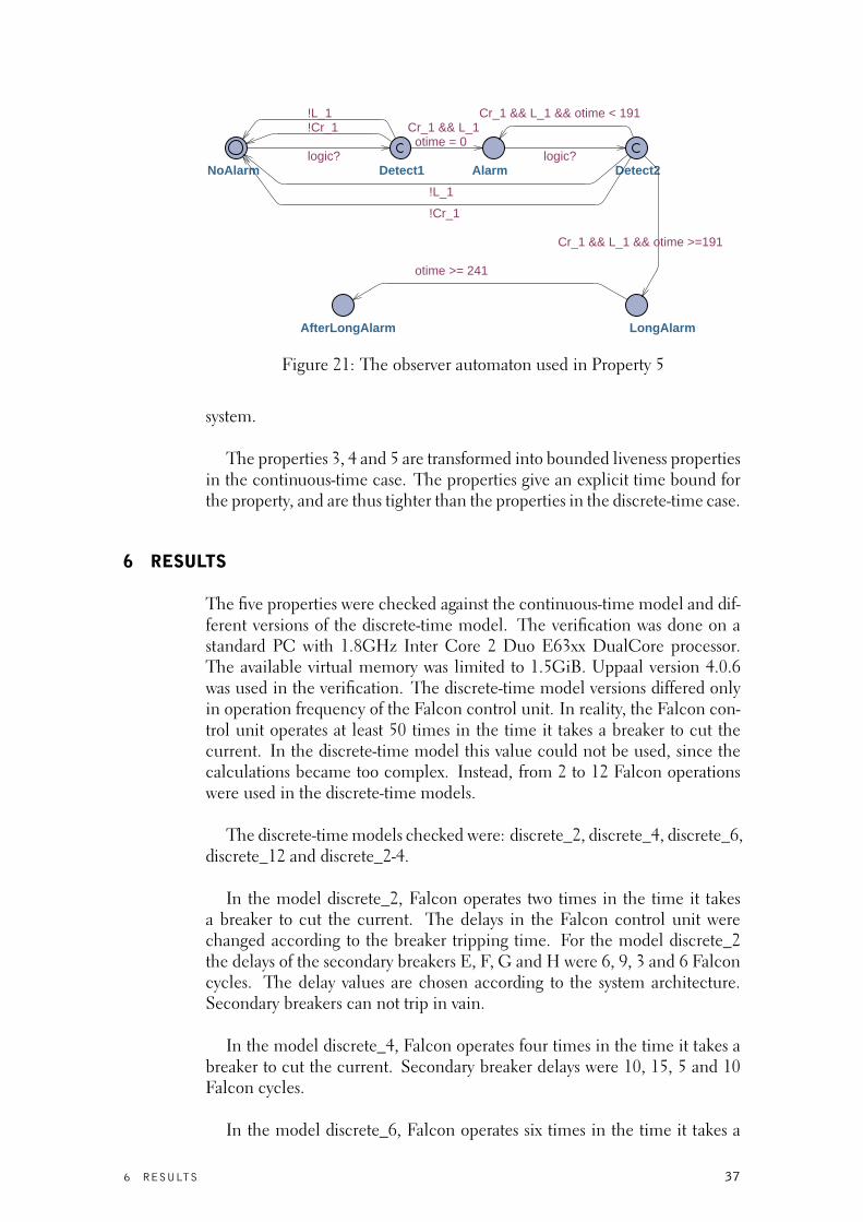
AfterLongAlarm LongAlarm

Detect1 Alarm Detect2NoAlarm

!L_1!Cr_1

!L_1

otime >= 241

!Cr_1

Cr_1 && L_1 && otime >=191

Cr_1 && L_1otime = 0

logic?

Cr_1 && L_1 && otime < 191

logic?

Figure 21: The observer automaton used in Property 5

system.

The properties 3, 4 and 5 are transformed into bounded liveness propertiesin the continuous-time case. The properties give an explicit time bound forthe property, and are thus tighter than the properties in the discrete-time case.

6 RESULTS

The five properties were checked against the continuous-time model and dif-ferent versions of the discrete-time model. The verification was done on astandard PC with 1.8GHz Inter Core 2 Duo E63xx DualCore processor.The available virtual memory was limited to 1.5GiB. Uppaal version 4.0.6was used in the verification. The discrete-time model versions differed onlyin operation frequency of the Falcon control unit. In reality, the Falcon con-trol unit operates at least 50 times in the time it takes a breaker to cut thecurrent. In the discrete-time model this value could not be used, since thecalculations became too complex. Instead, from 2 to 12 Falcon operationswere used in the discrete-time models.

The discrete-time models checked were: discrete_2, discrete_4, discrete_6,discrete_12 and discrete_2-4.

In the model discrete_2, Falcon operates two times in the time it takesa breaker to cut the current. The delays in the Falcon control unit werechanged according to the breaker tripping time. For the model discrete_2the delays of the secondary breakers E, F, G and H were 6, 9, 3 and 6 Falconcycles. The delay values are chosen according to the system architecture.Secondary breakers can not trip in vain.

In the model discrete_4, Falcon operates four times in the time it takes abreaker to cut the current. Secondary breaker delays were 10, 15, 5 and 10Falcon cycles.

In the model discrete_6, Falcon operates six times in the time it takes a

6 RESULTS 37

breaker to cut the current. Secondary breaker delays were 14, 21, 7 and 14Falcon cycles.

In the model discrete_12, Falcon operates twelve times in the time it takesa breaker to cut the current. Secondary breaker delays were 26, 39, 13 and26 Falcon cycles.

The model discrete_2-4 was such that breakers needed a minimum of 2cycles and a maximum of 4 cycles to trip. Secondary breaker delays were 10,15, 5 and 10 Falcon cycles.

The continuous-time model was such that breakers needed 50 time unitsto trip. Secondary breaker delays were 120, 190, 60 and 120 time units.

The running times were as follows:

discrete_2 discrete_4 discrete_6 discrete_12Property 1 1 min 11 s 8 min 29 s 32 min 22 s 16 h 27 minProperty 2 1 min 11 s 8 min 31 s 38 min 37 s 16 h 28 minProperty 3 1 min 19 s 9 min 30 s 43 min 19 s 19 h 10 minProperty 4 2 min 19 s 19 min 1 h 38 min > 20 hProperty 5 2 min 7 s 17 min 1 h 27 min Out of Memory

discrete_2-4Property 1 7 min 28 sProperty 2 7 min 25 sProperty 3 9 min 25 sProperty 4 19 min 13 sProperty 5 17 min 18 s

As a comparison, if a simplification to the Falcon logic is made in thediscrete-time model, so that no light signals exist, but the same functionalbehaviour is present, the following results were obtained. The simplifieddiscrete-time model is represented in Appedix C.

abs_discrete_2 abs_discrete_4 abs_discrete_6 abs_discrete_12Property 1 5 s 34 s 2 min 44 s 1 h 54 minProperty 2 5 s 34 s 2 min 43 s 1 h 53 minProperty 3 5 s 39 s 3 min 6 s 2 h 14 minProperty 4 10 s 1 min 22 s 7 min 19 s Out of MemoryProperty 5 10 s 1 min 23 s 7 min 47 s Out of Memory

abs_discrete_2-4Property 1 30 sProperty 2 30 sProperty 3 41 sProperty 4 1 min 22 sProperty 5 1 min 24 s

38 6 RESULTS

Results for the continuous-time case were the following:

continuous-modelProperty 1 30 min 18 sProperty 2 29 min 56 sProperty 3 1 h 6 minProperty 4 2 h 40 minProperty 5 2 h 39 min

As in the discrete-time case, the same logic simplification can also bemade in the continuous-time case. The simplified continuous-time modelis represented in Appedix D. The following results were obtained:

abs_continuous -modelProperty 1 1 min 33 sProperty 2 1 min 32 sProperty 3 4 min 30 sProperty 4 16 min 12 sProperty 5 16 min 15 s

We can make many observations from the results. Firstly, the checkedproperty itself has influence on the length of the verification in all models.Properties 1 and 2 seem to be the easiest, and properties 4 and 5 seem to bethe hardest. The properties that require an observer automaton take invari-ably more time to verify than the other properties. This is understandablebecause an additional automaton adds some complexity to the model.

Secondly, the frequency of the Falcon control unit operation in the discrete-time model had a great influence on the verification times. In the modeldiscrete_12 the properties 4 and 5 could not be verified within the used timeand memory limit, while in the model discrete_2 all properties could be ver-ified within a few minutes.

If the logic is simplified so that the same functional behaviour is preserved,while the number of inputs is decreased, the verification times decrease sub-stantially in both models. The properties 4 and 5 could still not be verifiedfor the discrete-time model discrete_12.

Also, the use of variable length cutting times in the model discrete_2-4did not result in longer verification times for any property compared to themodel discrete_4.

Finally, while the continuous-time model could not be verified in a partic-ularly short time, it covers all the behaviour of a discrete-time model operat-ing at a real-life frequency. Such a discrete-time model could not be verifiedbecause of its complexity.

6 RESULTS 39

7 CONCLUSIONS

In this work an electric arc protection system controlled by a programmablelogic controller (PLC) was modelled and verified. The used model check-ing tool was Uppaal. The UTU electric arc protection system was modelledin two different ways. The discrete-time model was based on counters anda controller operating at a specific rate. In the continuous-time model thecounters were replaced with clocks, and the controller was allowed to oper-ate at a varying frequency.

The properties requiring an observer automaton could not be checkedagainst the version of the discrete-time model with the most complexity, dis-crete_12. Either the memory limit of 1.5 GiB was reached or more than 20hours was needed for the verification. In addition, the checked discrete-timemodel versions were simpler than the real modelled system. To be exact, thereal controller operates more frequently than in the discrete-time model. Itis also hard to prove that the discrete-time model captures all the essentialbehaviour of the system.

The discrete-time model was not really the optimal model to be analyzedwith the real-time model checker Uppaal because of the discrete time. Up-paal is designed to work with real-time models, and this is why the continuous-time model proved to be more expressive.

The continuous-time model actually has more behaviour than the realcontroller. Therefore, if no unwanted behaviour could be observed in thecontinuous-time model, the real system must be working correctly as well.This is only true because the checked properties could be stated as invariantproperties i.e., properties that are true in all states of the model.

It can also be noticed that the continuous-time model simulates the discrete-time model operating at a realistic frequency. The set of execution traces ofthe continuous-time model covers the execution traces of the discrete-timemodel. In other words, the set of execution traces of the continuous-timemodel is a superset of the execution traces of the discrete-time model. Thecontinuous-time model can always choose to imitate the operation of thediscrete-time model.

As a general observation, the most difficult part of the modelling workwas to find the right abstraction level that captures the system behaviour ad-equately, and does not result in too complex verification. In Uppaal, therunning times of the verification increase rapidly as the number of inputvariables is increased. In the results, the logic simplification was done byremoving 3 of the 7 input variables of the Falcon control unit. This simplifi-cation led to significant decrease in running times. The external behaviourof the system did not change because of the simplification.

All TCTL specifications can not be stated in the subset of TCTL Uppaalsupports. Many specifications require the use of an additional observer au-

40 7 CONCLUSIONS

tomaton. The use and generation of these observer automata is not straight-forward, and the correctness of the observer automaton implementation isdifficult to assure.

In conclusion, Uppaal is suitable for the model checking of time-criticalsystems, but does not perform well if a lot of unconstrained input variablesare needed. Model checking is a valuable tool in the verification of safetyinstrumented systems.

Acknowledgements

This work was part of the research project Model-based safety evaluation ofautomation systems (MODSAFE). The project is part of the Finnish Re-search Programme on Nuclear Power Plant Safety 2007-2010 (SAFIR2010),funded by the State Nuclear Waste Management Fund (VYR).

I want to thank my supervisor Prof. Ilkka Niemelä and my instructor Do-cent Keijo Heljanko for their encouragement and guidance throughout thisstudy. I also want to thank for the opportunity to work here at the Departmentof Information and Computer Science.

REFERENCES

[1] R. Alur. Timed automata. In Computer Aided Verification, pages 8–22,1999.

[2] R. Alur, C. Courcoubetis, and D. L. Dill. Model-checking for real-timesystems. In Proceedings, Fifth Annual IEEE Symposium on Logic inComputer Science, pages 414–425, Philadelphia, Pennsylvania, June4–7 1990. IEEE Computer Society Press.

[3] R. Alur and D. L. Dill. A theory of timed automata. Theoretical Com-puter Science, 126(2):183–235, 1994.

[4] N. Bauer, S. Engell, R. Huuck, S. Lohmann, B. Lukoschus,M. Remelhe, and O. Stursberg. Verification of PLC programs givenas sequential function charts. In SoftSpez Final Report, pages 517–540,2004.

[5] G. Behrmann, J. Bengtsson, A. David, K. G. Larsen, P. Pettersson, andW. Yi. Uppaal implementation secrets. In FTRTFT ’02: Proceedings ofthe 7th International Symposium on Formal Techniques in Real-Timeand Fault-Tolerant Systems, pages 3–22, London, UK, 2002. Springer-Verlag.

[6] G. Behrmann, A. David, and K. G. Larsen. A tutorial on UPPAAL. InM. Bernardo and F. Corradini, editors, Formal Methods for the De-sign of Real-Time Systems: 4th International School on Formal Meth-

REFERENCES 41

ods for the Design of Computer, Communication, and Software Sys-tems, SFM-RT 2004, number 3185 in LNCS, pages 200–236. Springer-Verlag, September 2004.

[7] J. Bengtsson, W. O. D. Griffioen, K. J. Kristoffersen, K. G. Larsen,F. Larsson, P. Pettersson, and W. Yi. Verification of an audio protocolwith bus collision using UPPAAL. In R. Alur and T. A. Henzinger, edi-tors, Proceedings of the Eighth International Conference on ComputerAided Verification CAV, pages 244–256, New Brunswick, NJ, USA, /1996. Springer-Verlag.

[8] J. Bengtsson and W. Yi. Timed automata: Semantics, algorithms andtools. In J. Desel, W. Reisig, and G. Rozenberg, editors, Lectures onConcurrency and Petri Nets, volume 3098 of Lecture Notes in Com-puter Science, pages 87–124. Springer-Verlag, 2003.

[9] A. Biere, A. Cimatti, E. M. Clarke, and Y. Zhu. Symbolic model check-ing without BDDs. In R. Cleaveland, editor, Tools and Algorithms forConstruction and Analysis of Systems, 5th International Conference,TACAS ’99, Held as Part of the European Joint Conferences on theTheory and Practice of Software, ETAPS’99, Amsterdam, The Nether-lands, March 22-28, 1999, Proceedings, volume 1579 of Lecture Notesin Computer Science, pages 193–207. Springer-Verlag, 1999.

[10] A. Biere, K. Heljanko, T. Junttila, T. Latvala, and V. Schuppan. Lin-ear encodings of bounded LTL model checking. Logical Methods inComputer Science, 2(5:5), 2006. (doi: 10.2168/LMCS-2(5:5)2006).

[11] E. M. Bortnik, N. Trcka, A. Wijs, B. Luttik, J. M. van de Mortel-Fronczak, J. C. M. Baeten, W. Fokkink, and J. E. Rooda. Analyzinga χ model of a turntable system using Spin, CADP and Uppaal. J. Log.Algebr. Program., 65(2):51–104, 2005.

[12] B. Brard, P. Bouyer, and A. Petit. Analysing the PGM Protocol with UP-PAAL. In Proc. 2nd Workshop on Real-Time Tools (RT-TOOLS’02).Technical Report 2002-025, Uppsala University, Sweden, 2002.

[13] N. C. W. M. Braspenning, E. M. Bortnik, J. M. van de Mortel-Fronczak,and J. E. Rooda. Model-based system analysis using Chi and Uppaal:An industrial case study. Comput. Ind., 59(1):41–54, 2008.

[14] M. C. Browne, E. M. Clarke, and O. Grumberg. Characterizing Kripkestructures in temporal logic. In The International Joint Conference ontheory and practice of software development on TAPSOFT ’87, pages256–270, London, UK, 1987. Springer-Verlag.

[15] K. Cerans. Decidability of bisimulation equivalences for parallel timerprocesses. In G. von Bochmann and D. K. Probst, editors, ComputerAided Verification, Fourth International Workshop, CAV ’92, Montreal,Canada, June 29 - July 1, 1992, Proceedings, volume 663 of LectureNotes in Computer Science, pages 302–315. Springer-Verlag, 1992.

42 REFERENCES

[16] Z. Chaochen. Duration calculus, a logical approach to real-time sys-tems. In A. M. Haeberer, editor, Algebraic Methodology and SoftwareTechnology, 7th International Conference, AMAST ’98, Amazonia,Brasil, January 4-8, 1999, Proceedings, volume 1548 of Lecture Notesin Computer Science, pages 1–7. Springer-Verlag, 1998.

[17] E. Clarke, O. Grumberg, S. Jha, Y. Lu, and H. Veith. Progress on thestate explosion problem in model checking. Lecture Notes in Com-puter Science, 2000:176–194, 2001.

[18] P. R. D’Argenio, J.-P. Katoen, T. C. Ruys, and G. J. Tretmans. Thebounded retransmission protocol must be on time! In E. Brinksma, ed-itor, Tools and Algorithms for the Construction and Analysis of Systems,pages 416–432, Enschede, The Netherlands, 1997. Springer-Verlag,Lecture Notes in Computer Science 1217.

[19] D. L. Dill. Timing assumptions and verification of finite-state concur-rent systems. In J. Sifakis, editor, Automatic Verification Methods forFinite State Systems, volume 407 of Lecture Notes in Computer Sci-ence, pages 197–212. Springer-Verlag, 1989.

[20] E. M. Clarke, Jr., O. Grumberg, and D. A. Peled. Model Checking.The MIT Press, 1999.

[21] E. A. Emerson. Temporal and modal logic. pages 995–1072, The MITPress, 1990.

[22] J.-C. Fernandez, H. Garavel, A. Kerbrat, L. Mounier, R. Mateescu, andM. Sighireanu. CADP: A protocol validation and verification toolbox.In R. Alur and T. A. Henzinger, editors, Proceedings of the EighthInternational Conference on Computer Aided Verification CAV, vol-ume 1102, pages 437–440, New Brunswick, NJ, USA, / 1996. Springer-Verlag.

[23] W. M. Goble and H. Cheddie. Safety Instrumented Systems Verifi-cation: Practical Probabilistic Calculations. ISA-Instrumentation, Sys-tems, and Automation Society, NC, USA, 2005.

[24] P. Godefroid. Partial-Order Methods for the Verification of ConcurrentSystems - An Approach to the State-Explosion Problem, volume 1032of Lecture Notes in Computer Science. Springer-Verlag, 1996.

[25] J. F. Groote, J. Pang, and A. G. Wouters. Analysis of a distributed systemfor lifting trucks. Technical Report UMI Order Number: SEN-R0111,CWI (Centre for Mathematics and Computer Science), Amsterdam,The Netherlands, 2001.

[26] K. Havelund, K. G. Larsen, and A. Skou. Formal verification of a powercontroller using the real-time model checker UPPAAL. Lecture Notesin Computer Science, 1601:277–298, 1999.

REFERENCES 43

[27] K. Havelund, A. Skou, K. G. Larsen, and K. Lund. Formal model-ing and analysis of an audio/video protocol: an industrial case studyusing uppaal. In RTSS ’97: Proceedings of the 18th IEEE Real-TimeSystems Symposium (RTSS ’97), pages 2–13, Washington, DC, USA,1997. IEEE Computer Society.

[28] M. Hendriks, B. van den Nieuwelaar, and F. Vaandrager. Modelchecker aided design of a controller for a wafer scanner. Int. J. Softw.Tools Technol. Transf., 8(6):633–647, 2006.

[29] T. A. Henzinger, X. Nicollin, J. Sifakis, and S. Yovine. Symbolic modelchecking for real-time systems. Inf. Comput., 111(2):193–244, 1994.

[30] A. Hessel, K. G. Larsen, B. Nielsen, P. Pettersson, and A. Skou. Time-optimal real-time test case generation using Uppaal. In A. Petrenkoand A. Ulrich, editors, Formal Approaches to Software Testing, ThirdInternational Workshop on Formal Approaches to Testing of Software,FATES 2003, Montreal, Quebec, Canada, October 6th, 2003, volume2931 of Lecture Notes in Computer Science, pages 114–130. Springer,2003.

[31] G. J. Holzmann. The model checker SPIN. IEEE Transactions onSoftware Engineering, 23(5):279–295, 1997.

[32] R. Huuck. Software Verification for Programmable Logic Controllers.PhD thesis, Christian-Albrechts-Universität zu Kiel, Germany, 2003.

[33] H. E. Jensen, K. G. Larsen, and A. Skou. Modelling and analysis of acollision avoidance protocol using SPIN and UPPAAL. In The SecondWorkshop on the SPIN Verification System, volume 32 of DIMACS,Series in Discrete Mathematics and Theoretical Computer Science.American Mathematical Society, 1996.

[34] K. G. Larsen, P. Pettersson, and W. Yi. Uppaal in a nutshell. STTT,1(1-2):134–152, 1997.

[35] K. G. Larsen and Y. Wang. Time-abstracted bisimulation: Implicit spec-ifications and decidability. Information and Computation, 134(2):75–101, 1997.

[36] M. Laursen, R. G. Madsen, and S. K. Mortensen. Verifying distributedLEGO RCX programs using UPPAAL. Technical report, Institute ofComputer Science, Aalborg University, 1999.

[37] M. Lindahl, P. Pettersson, and W. Yi. Formal design and analysis of agear controller. In TACAS ’98: Proceedings of the 4th InternationalConference on Tools and Algorithms for Construction and Analysis ofSystems, pages 281–297, London, UK, 1998. Springer-Verlag.

[38] A. Mader. Precise timing analysis of PLC applications two small exam-ples. Unpublished manuscript. Available from iteseer.ist.psu.edu/mader00pre ise.html.

44 REFERENCES

[39] R. Milner. Communication and concurrency. Prentice-Hall, Inc., Up-per Saddle River, NJ, USA, 1989.

[40] X. Nicollin and J. Sifakis. The algebra of timed processes, ATP: theoryand application. Inf. Comput., 114(1):131–178, 1994.

[41] J. Pang, B. Karstens, and W. Fokkink. Analyzing the redesign of a dis-tributed lift system in UPPAAL. In J. S. Dong and J. Woodcock, editors,ICFEM, volume 2885 of Lecture Notes in Computer Science, pages504–522. Springer-Verlag, 2003.

[42] G. M. Reed and A. W. Roscoe. A timed model for communicatingsequential processes. Theor. Comput. Sci., 58(1-3):249–261, 1988.

[43] G. Rodriguez-Navas, J. Proenza, and H. Hansson. Using UPPAAL tomodel and verify a clock synchronization protocol for the controllerarea network. ETFA 2005. 10th IEEE Conference on Emerging Tech-nologies and Factory Automation, 2, 2005.

[44] G. Rodriguez-Navas, J. Proenza, and H. Hansson. An UPPAAL modelfor formal verification of master/slave clock synchronization over thecontroller area network. Factory Communication Systems, 2006 IEEEInternational Workshop on, pages 3–12, June 27, 2006.

[45] J. Valkonen, V. Pettersson, K. Björkman, J.-E. Holmberg, M. Koskimies,K. Heljanko, and I. Niemelä. Model-based analysis of an arc protectionand an emergency cooling system. VTT Working Papers 93, VTT Tech-nical Research Centre of Finland, Espoo, 2008.

[46] A. Valmari. The state explosion problem. In W. Reisig and G. Rozen-berg, editors, Petri Nets, volume 1491 of Lecture Notes in ComputerScience, pages 429–528. Springer-Verlag, 1996.

[47] D. A. van Beek, K. L. Man, M. A. Reniers, J. E. Rooda, and R. R. H.Schiffelers. Syntax and consistent equation semantics of hybrid Chi. J.Log. Algebr. Program., 68(1-2):129–210, 2006.

[48] F. Wang. Red: Model-checker for timed automata with clock-restrictiondiagram. In P. Pettersson and S. Yovine, editors, Workshop on Real-Time Tools, Aalborg University Denmark. number 2001-014 in Tech-nical Report. Uppsala University, 2001.

[49] H. X. Willems. Compact timed automata for PLC programs. Tech-nical Report CSI-R9925, University of Nijmegen, Computing ScienceInstitute, 1999.

[50] W. Yi. CCS + Time = An interleaving model for real time systems.In Proceedings of the 18th international colloquium on Automata, lan-guages and programming, pages 217–228, New York, NY, USA, 1991.Springer-Verlag New York, Inc.

[51] S. Yovine. Kronos: A verification tool for real-time systems. STTT,1(1-2):123–133, 1997.

REFERENCES 45

A FALCON CASE: DISCRETE-TIME MODEL RELATED CODE

The global declarations used in the model checking of the falcon case indiscrete time are listed below.bool tr1, tr2, tr3, tr4;bool relay1, relay2, relay3, relay4;broad ast han he k;bool breakerA uts = false;bool breakerB uts = false;bool breakerC uts = false;bool breakerD uts = false;bool breakerE uts = false;bool breakerF uts = false;bool breakerG uts = false;bool breakerH uts = false;

The system declarations (parallel composition descriptions) of the caseare the following://Parameters: Se ondary breaker delaysFal on = Fal onsystem(6, 9, 3, 6);//Parameters:// 1. the tria /relay signal// 2. minimum utting time// 3. maximum utting time// 4. boolean variable Breaker-has- utBreakerA = Breaker(tr1, 2, 2, breakerA uts);BreakerB = Breaker(tr2, 2, 2, breakerB uts);BreakerC = Breaker(tr3, 2, 2, breakerC uts);BreakerD = Breaker(tr4, 2, 2, breakerD uts);BreakerE = BreakerSe (relay1, 2, 2, breakerE uts);BreakerF = BreakerSe (relay2, 2, 2, breakerF uts);BreakerG = BreakerSe (relay3, 2, 2, breakerG uts);BreakerH = BreakerSe (relay4, 2, 2, breakerH uts);// List one or more pro esses to be omposed into a system.system Fal on, BreakerA, BreakerB, BreakerC, BreakerD,BreakerE, BreakerF, BreakerG, BreakerH;

The Falcon control unit automaton related code is the following://input signalsbool Cr_1, Cr_2, Cr_3a, Cr_3b, L_1, L_2, L_3;46 A FALCON CASE: DISCRETE-TIME MODEL RELATED CODE

int rel1buffer = 0;int rel2buffer = 0;int rel3buffer = 0;int rel4buffer = 0;int zone1get urrent, zone2get urrent, zone3get urrent; lo k time;//Get Fal on system inputs from suggested inputs and// al ulate outputsvoid getvalues(bool Cr_1_S, bool Cr_2_S, bool Cr_3a_S,bool Cr_3b_S, bool L_1_S, bool L_2_S, bool L_3_S ) {zone1get urrent = !(breakerA uts || ((breakerE uts ||breakerH uts) & (breakerC uts|| breakerD uts ||breakerG uts || breakerF uts)));zone2get urrent = !(breakerB uts || ((breakerE uts ||breakerH uts) & (breakerC uts|| breakerD uts ||breakerG uts || breakerF uts)));zone3get urrent = !((breakerC uts || breakerE uts ||breakerH uts) & (breakerD uts || breakerF uts ||breakerG uts));Cr_1 = Cr_1_S & zone1get urrent;Cr_2 = Cr_2_S & zone2get urrent;Cr_3a = Cr_3a_S & !breakerC uts & zone3get urrent;Cr_3b = Cr_3b_S & !breakerD uts & zone3get urrent;L_1 = L_1_S;L_2 = L_2_S;L_3 = L_3_S;// get the outputstr1 = Cr_1 & L_1;tr2 = Cr_2 & L_2;tr3 = (Cr_1 & L_1) || (Cr_2 & L_2) ||((Cr_3a || Cr_3b) & L_3);tr4 = ((Cr_3a || Cr_3b) & L_3);relay1 = (Cr_1 & L_1) || (Cr_2 & L_2) ;relay2 = (Cr_1 & L_1) || (Cr_2 & L_2) ;relay3 = ((Cr_3a || Cr_3b) & L_3);relay4 = ((Cr_3a || Cr_3b) & L_3);A FALCON CASE: DISCRETE-TIME MODEL RELATED CODE 47

// al ulate ontinuous alarm lengths (relXbuffer) and// update slow relay-output values (relayX)if (relay1 == 0) {rel1buffer =0;}if (rel1buffer < r1 & relay1 == 1) {rel1buffer++;relay1=0;}if (rel1buffer == r1 && relay1 == 1){relay1 = 1;}if (relay2 == 0) {rel2buffer =0;}if (rel2buffer < r2 & relay2 == 1) {rel2buffer++;relay2=0;}if (rel2buffer == r2 && relay2 == 1){relay2 = 1;}if (relay3 == 0) {rel3buffer =0;}if (rel3buffer < r3 & relay3 == 1) {rel3buffer++;relay3=0;}if (rel3buffer == r3 && relay3 == 1){relay3 = 1;}if (relay4 == 0) {rel4buffer =0;}if (rel4buffer < r4 & relay4 == 1) {rel4buffer++;relay4=0;}if (rel4buffer == r4 && relay4 == 1){relay4 = 1;}48 A FALCON CASE: DISCRETE-TIME MODEL RELATED CODE

//reset the inputsCr_1=0;Cr_2=0;Cr_3a=0;Cr_3b=0;L_1=0;L_2=0;L_3=0;}

A FALCON CASE: DISCRETE-TIME MODEL RELATED CODE 49

B FALCON CASE: CONTINUOUS-TIME MODEL RELATED CODE

The global declarations used in the model checking of the falcon case incontinuous time are listed below.// Pla e global de larations here.bool tr1, tr2, tr3, tr4;bool relay1, relay2, relay3,relay4;broad ast han logi ;broad ast han break; han event;bool breakerA uts = false;bool breakerB uts = false;bool breakerC uts = false;bool breakerD uts = false;bool breakerE uts = false;bool breakerF uts = false;bool breakerG uts = false;bool breakerH uts = false;bool Cr_1, Cr_2, Cr_3a, Cr_3b, L_1, L_2, L_3;

The system declarations (parallel composition descriptions) of the caseare the following:Fal on = Fal onsystem();BreakerA = Breaker(tr1, 50, 50, breakerA uts);BreakerB = Breaker(tr2, 50, 50, breakerB uts);BreakerC = Breaker(tr3, 50, 50, breakerC uts);BreakerD = Breaker(tr4, 50, 50, breakerD uts);// parameters:// delay-time// signal that needs to stay on for the time of delay// mintime of breaker ut// maxtime of breaker ut// the variable that is set when breakBreakerE = DelayAndBreaker(102, relay1, 40, 50, breakerE uts);BreakerF = DelayAndBreaker(153, relay2, 40, 50, breakerF uts);BreakerG = DelayAndBreaker(51, relay3, 40, 50, breakerG uts);BreakerH = DelayAndBreaker(102, relay4, 40, 50, breakerH uts);// List one or more pro esses to be omposed into a system.system Fal on, BreakerA, BreakerB, BreakerC, BreakerD, BreakerE,

50 B FALCON CASE: CONTINUOUS-TIME MODEL RELATED CODE

BreakerF, BreakerG, BreakerH, Environment, Observer;The Falcon control unit automaton related code is the following:int zone1get urrent, zone2get urrent, zone3get urrent;//Get Fal on system inputs from suggested inputs and// al ulate outputsvoid getvalues(bool Cr_1_S, bool Cr_2_S, bool Cr_3a_S,bool Cr_3b_S, bool L_1_S, bool L_2_S, bool L_3_S) {// al ulate possible input valueszone1get urrent = !(breakerA uts || ((breakerE uts ||breakerH uts) & (breakerC uts|| breakerD uts ||breakerG uts || breakerF uts)));zone2get urrent = !(breakerB uts || ((breakerE uts ||breakerH uts) & (breakerC uts|| breakerD uts ||breakerG uts || breakerF uts)));zone3get urrent = !((breakerC uts || breakerE uts ||breakerH uts) & (breakerD uts ||breakerF uts || breakerG uts));Cr_1 = Cr_1_S & zone1get urrent;Cr_2 = Cr_2_S & zone2get urrent;Cr_3a = Cr_3a_S & zone3get urrent & !breakerC uts;Cr_3b = Cr_3b_S & zone3get urrent & !breakerD uts;L_1= L_1_S;L_2=L_2_S;L_3=L_3_S;// get the outputstr1 = Cr_1 & L_1;tr2 = Cr_2 & L_2;tr3 = (Cr_1 & L_1) || (Cr_2 & L_2) ||((Cr_3a || Cr_3b) & L_3);tr4 = ((Cr_3a || Cr_3b) & L_3);relay1 = (Cr_1 & L_1) || (Cr_2 & L_2) ;relay2 = (Cr_1 & L_1) || (Cr_2 & L_2) ;relay3 = ((Cr_3a || Cr_3b) & L_3);relay4 = ((Cr_3a || Cr_3b) & L_3);}

B FALCON CASE: CONTINUOUS-TIME MODEL RELATED CODE 51

C FALCON CASE: THE DISCRETE-TIME SIMPLIFIED MODEL

Here the discrete-time model with a logic simplification is represented. Onlythe modified parts of the model are shown. Otherwise the model remains un-changed. The Falcon control unit automaton of the simplified discrete-timemodel is in Figure 22.

Idletime<= 1

Cr_1_S: int[0,1], Cr_2_S: int[0,1], Cr_3_S: int[0,1]time==1

check!getvalues(Cr_1_S, Cr_2_S, Cr_3_S), time=0

Figure 22: The Falcon control unit of the simplified discrete-time model

The global declarations used in the model checking are listed below.bool tr1, tr2, tr3, tr4;bool relay1, relay2, relay3, relay4;broad ast han he k;bool breakerA uts = false;bool breakerB uts = false;bool breakerC uts = false;bool breakerD uts = false;bool breakerE uts = false;bool breakerF uts = false;bool breakerG uts = false;bool breakerH uts = false;bool was_Cr_1, Now_CrL;The Falcon control unit automaton related code is the following:// observer variablesbool Cr1_L1_was;bool wasalarm;//Real input valuesbool Cr_1, Cr_2, Cr_3;int rel1buffer = 0;int rel2buffer = 0;

52 C FALCON CASE: THE DISCRETE-TIME SIMPLIFIED MODEL

int rel3buffer = 0;int rel4buffer = 0;int zone1get urrent, zone2get urrent, zone3get urrent; lo k time;//Get Fal on system inputs from suggested inputs and// al ulate outputsvoid getvalues(bool Cr_1_S, bool Cr_2_S, bool Cr_3_S) {zone1get urrent = !(breakerA uts || ((breakerE uts|| breakerH uts) & (breakerC uts|| breakerD uts|| breakerG uts || breakerF uts)));zone2get urrent = !(breakerB uts || ((breakerE uts|| breakerH uts) & (breakerC uts|| breakerD uts|| breakerG uts || breakerF uts)));zone3get urrent = !((breakerC uts || breakerE uts ||breakerH uts) & (breakerD uts || breakerF uts ||breakerG uts));Cr_1 = Cr_1_S & zone1get urrent;Cr_2 = Cr_2_S & zone2get urrent;Cr_3 = Cr_3_S & zone3get urrent &(!breakerC uts || !breakerD uts);if (Cr_1) was_Cr_1 = true;if (Cr_1) Now_CrL = true;if (!Cr_1) Now_CrL = false;// get the outputstr1 = Cr_1;tr2 = Cr_2;tr3 = Cr_1 || Cr_2 || Cr_3;tr4 = Cr_3;relay1 = tr1 || tr2 ;relay2 = relay1;relay3= tr4;relay4 = tr4;if (relay1 == 0) {rel1buffer =0;}if (rel1buffer < r1 & relay1 == 1) {rel1buffer++;relay1 =0;}if (rel1buffer == r1 && relay1 == 1){C FALCON CASE: THE DISCRETE-TIME SIMPLIFIED MODEL 53

relay1 = 1;}if (relay2 == 0) {rel2buffer =0;}if (rel2buffer < r2 & relay2 == 1) {rel2buffer++;relay2 =0;}if (rel2buffer == r2 && relay2 == 1){relay2 = 1;}if (relay3 == 0) {rel3buffer =0;}if (rel3buffer < r3 & relay3 == 1) {rel3buffer++;relay3 =0;}if (rel3buffer == r3 && relay3 == 1){relay3 = 1;}if (relay4 == 0) {rel4buffer =0;}if (rel4buffer < r4 & relay4 == 1) {rel4buffer++;relay4 =0;}if (rel4buffer == r4 && relay4 == 1){relay4 = 1;}// reset the inputs:Cr_1=0;Cr_2=0;Cr_3=0;}

54 C FALCON CASE: THE DISCRETE-TIME SIMPLIFIED MODEL

D FALCON CASE: THE CONTINUOUS-TIME SIMPLIFIED MODEL

Here the continuous-time model with a logic simplification is represented.Only the modified parts of the model are shown. Otherwise the model re-mains unchanged. The Falcon control unit automaton of the simplifiedcontinuous-time model is in Figure 23.

GotEventIdle

Cr_1_S: int[0,1], Cr_2_S: int[0,1], Cr_3_S: int[0,1]

logic!getvalues(Cr_1_S, Cr_2_S, Cr_3_S)

event?

Figure 23: The Falcon control unit of the simplified continuous-time model

The global declarations used in the model checking are listed below.bool tr1, tr2, tr3, tr4;bool relay1, relay2, relay3,relay4;broad ast han logi ;broad ast han break; han event;bool breakerA uts = false;bool breakerB uts = false;bool breakerC uts = false;bool breakerD uts = false;bool breakerE uts = false;bool breakerF uts = false;bool breakerG uts = false;bool breakerH uts = false;bool Cr_1, Cr_2, Cr_3;bool was_Cr_1;The Falcon control unit automaton related code is the following:int zone1get urrent, zone2get urrent, zone3get urrent;//Get Fal on system inputs from suggested inputs and// al ulate outputsvoid getvalues(bool Cr_1_S, bool Cr_2_S, bool Cr_3_S) {// al ulate possible input valueszone1get urrent = !(breakerA uts || ((breakerE uts|| breakerH uts) & (breakerC uts|| breakerD uts|| breakerG uts || breakerF uts)));zone2get urrent = !(breakerB uts || ((breakerE uts

D FALCON CASE: THE CONTINUOUS-TIME SIMPLIFIED MODEL 55

|| breakerH uts) & (breakerC uts|| breakerD uts|| breakerG uts || breakerF uts)));zone3get urrent = !((breakerC uts || breakerE uts|| breakerH uts) & (breakerD uts || breakerF uts|| breakerG uts));Cr_1 = Cr_1_S & zone1get urrent;Cr_2 = Cr_2_S & zone2get urrent;Cr_3 = Cr_3_S & zone3get urrent &(!breakerC uts || !breakerD uts);if (Cr_1) was_Cr_1 = true;// get the outputstr1 = Cr_1;tr2 = Cr_2;tr3 = Cr_1 || Cr_2 || Cr_3;tr4 = Cr_3;relay1 = tr1 || tr2 ;relay2 = relay1;relay3 = tr4;relay4 = tr4;}

56 D FALCON CASE: THE CONTINUOUS-TIME SIMPLIFIED MODEL

TKK REPORTS IN INFORMATION AND COMPUTER SCIENCE

TKK-ICS-R1 Nikolaj Tatti, Hannes Heikinheimo

Decomposable Families of Itemsets. May 2008.

TKK-ICS-R2 Ville Viitaniemi, Jorma Laaksonen

Evaluation of Techniques for Image Classification, Object Detection and Object

Segmentation. June 2008.

ISBN 978-951-22-9444-2 (Print)

ISBN 978-951-22-9445-9 (Online)

ISSN 1797-5034 (Print)

ISSN 1797-5042 (Online)

ab - tcs.hut.fi · tkk reports in information and computer science ... 5 case study: falcon 24 ......

Documents