MANE 4240/ CIVL 4240: Introduction to Finite Elements

Abaqus Handout

Professor Suvranu De Department of Mechanical, Aerospace

and Nuclear Engineering

© Rensselaer Polytechnic Institute

2

Table of Contents 1. Introduction .................................................................................................................................. 4 2. Abaqus SE Installation Instructions ............................................................................................. 5 3. Introduction to Abaqus/CAE ........................................................................................................ 6 

3.1 Starting Abaqus/CAE ............................................................................................................. 7 3.2 Components of the main window ........................................................................................... 7 3.3 Starting Abaqus command .................................................................................................... 10 

4. TRUSS EXAMPLE: Analysis of an overhead hoist .................................................................. 12 4.1 Creating part ......................................................................................................................... 13 4.2 Creating material .................................................................................................................. 17 4.4 Defining the assembly .......................................................................................................... 19 4.5 Configuring analysis ............................................................................................................. 20 4.6 Applying boundary conditions and loads to the model ........................................................ 23 4.7 Meshing the model ............................................................................................................... 25 4.8 Creating an analysis job ........................................................................................................ 27 4.9 Checking the model .............................................................................................................. 28 4.10 Running the analysis ........................................................................................................... 29 4.11 Postprocessing with Abaqus/CAE ...................................................................................... 29 

5. 2D EXAMPLE: A rectangular plate with a hole in 2D plane stress .......................................... 35 5.1 Creating a part ...................................................................................................................... 36 5.2 Creating a material................................................................................................................ 36 5.3 Defining and assigning section properties ............................................................................ 37 5.4 Defining the assembly .......................................................................................................... 38 5.5 Configuring your analysis .................................................................................................... 38 5.6 Applying boundary conditions and loads to the model ........................................................ 38 5.7 Meshing ................................................................................................................................ 40 5.8 Remeshing and changing element types ............................................................................... 41 5.9 Creating an analysis job ........................................................................................................ 43 5.10 Checking the model ............................................................................................................ 43 5.11 Running the analysis ........................................................................................................... 44 5.12 Postprocessing with Abaqus/CAE ...................................................................................... 44 

5.12.1 Generating solution contours ....................................................................................... 45 5.12.2. Generating report of Field Outputs ............................................................................. 46 

6. 3D EXAMPLE: Analysis of 3D elastic solid ............................................................................. 48 6.1 Creating the cube .................................................................................................................. 49 6.2 Adding the flange to the base feature ................................................................................... 50 6.3 Creating a material................................................................................................................ 51 6.4 Defining a section ................................................................................................................. 51 6.5 Assigning the section ............................................................................................................ 52 6.6 Assembling the model by creating an instance of the hinge ................................................ 52 6.7 Defining analysis steps ......................................................................................................... 52 6.8 Selecting a degree of freedom to monitor ............................................................................ 54 6.9 Constraining the hinge .......................................................................................................... 54 6.10 Applying the pressure and the concentrated load to the hinge ........................................... 55 6.11 Meshing the assembly ........................................................................................................ 55 

6.11.1 Partitioning the model ................................................................................................. 56 6.11.2 Assigning the Abaqus element type ............................................................................ 57 

3

6.11.3 Seeding the part instances............................................................................................ 58 6.11.4 Meshing the assembly ................................................................................................. 58 

6.12 Creating and submitting a job ............................................................................................. 58 6.13 Viewing the results of your analysis ................................................................................... 60 

4

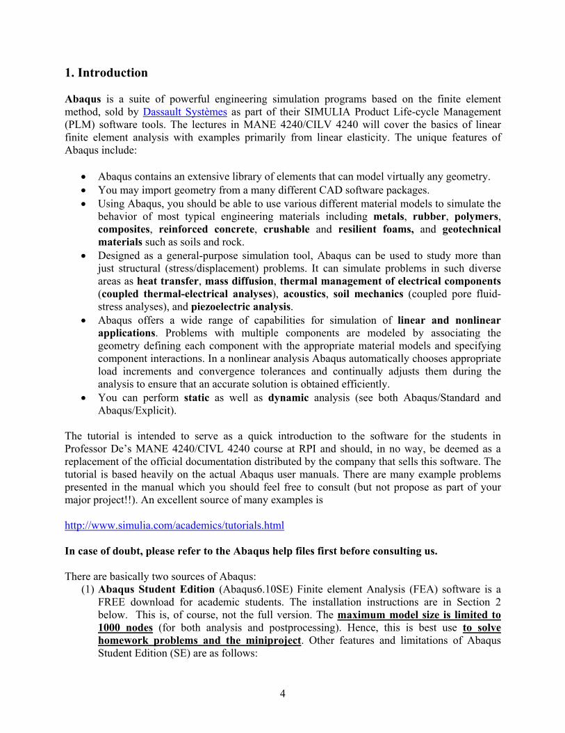
1. Introduction Abaqus is a suite of powerful engineering simulation programs based on the finite element method, sold by Dassault Systèmes as part of their SIMULIA Product Life-cycle Management (PLM) software tools. The lectures in MANE 4240/CILV 4240 will cover the basics of linear finite element analysis with examples primarily from linear elasticity. The unique features of Abaqus include:

Abaqus contains an extensive library of elements that can model virtually any geometry. You may import geometry from a many different CAD software packages. Using Abaqus, you should be able to use various different material models to simulate the

behavior of most typical engineering materials including metals, rubber, polymers, composites, reinforced concrete, crushable and resilient foams, and geotechnical materials such as soils and rock.

Designed as a general-purpose simulation tool, Abaqus can be used to study more than just structural (stress/displacement) problems. It can simulate problems in such diverse areas as heat transfer, mass diffusion, thermal management of electrical components (coupled thermal-electrical analyses), acoustics, soil mechanics (coupled pore fluid-stress analyses), and piezoelectric analysis.

Abaqus offers a wide range of capabilities for simulation of linear and nonlinear applications. Problems with multiple components are modeled by associating the geometry defining each component with the appropriate material models and specifying component interactions. In a nonlinear analysis Abaqus automatically chooses appropriate load increments and convergence tolerances and continually adjusts them during the analysis to ensure that an accurate solution is obtained efficiently.

You can perform static as well as dynamic analysis (see both Abaqus/Standard and Abaqus/Explicit).

The tutorial is intended to serve as a quick introduction to the software for the students in Professor De’s MANE 4240/CIVL 4240 course at RPI and should, in no way, be deemed as a replacement of the official documentation distributed by the company that sells this software. The tutorial is based heavily on the actual Abaqus user manuals. There are many example problems presented in the manual which you should feel free to consult (but not propose as part of your major project!!). An excellent source of many examples is http://www.simulia.com/academics/tutorials.html In case of doubt, please refer to the Abaqus help files first before consulting us. There are basically two sources of Abaqus:

(1) Abaqus Student Edition (Abaqus6.10SE) Finite element Analysis (FEA) software is a FREE download for academic students. The installation instructions are in Section 2 below. This is, of course, not the full version. The maximum model size is limited to 1000 nodes (for both analysis and postprocessing). Hence, this is best use to solve homework problems and the miniproject. Other features and limitations of Abaqus Student Edition (SE) are as follows:

5

The Abaqus Student Edition consists of Abaqus/Standard, Abaqus/Explicit, and

Abaqus/CAE only. Full HTML documentation is included. Perpetual License (no term, no license manager) Abaqus SE model databases are compatible with other academically licensed versions

of Abaqus (the Research and Teaching Editions) but not with commercially licensed versions of Abaqus.

More information: http://www.simulia.com/academics/student.html

(2) The full version (Abaqus 6.10), with no limitations on model size or modules is available for download from the RPI software repository. To access this, please go to http://www.rpi.edu/dept/arc/web/software/sw_available.html#abaqus and apply for a license. Shortly thereafter you will receive an email with the link to the instructions on how to install Abaqus on your machine. Since there is no limitation on the number of nodes, use this, if necessary, only for the major project. However, you are encouraged to choose a project that can be accomplished within the free student version rather than this full version of Abaqus. This is because the number of licenses for this full version is very limited. Also, this version is used not only for education but extensively for research. Currently we have 50 tokens; however, the CAE has 4 licenses. Hence, if many of you try to access this at the same time, the licenses will run out and you will be denied access. Be considerate and plan ahead so as not to inconvenience others. Keep in mind that This Abaqus Software cannot be used for commercial purposes. You cannot distribute this Abaqus Software to anyone. This Abaqus Software must be removed from your computer when you leave the

Rensselaer community. Please DO NOT request us to set Abaqus up for you. 2. Abaqus SE Installation Instructions Dassault Systèmes offers a FREE download. For detail download instructions visit: http://academy.3ds.com/simulia/freese The request for the Abaqus SE download will be reviewed within 2-5 business days, at which time you will be given additional instructions via email.

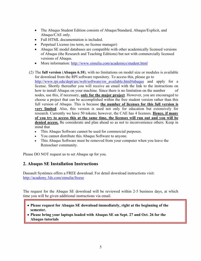
Please request for Abaqus SE download immediately, right at the beginning of the semester.

Please bring your laptops loaded with Abaqus SE on Sept. 27 and Oct. 26 for the Abaqus tutorials

6

System requirements

Operating system: Windows XP, Windows Vista, and Windows 7 Processor: Pentium 4 or higher Web browser: Internet Explorer 6, 7, or 8; Firefox 2.0, 3.0, or 3.5 Minimum disk space for installation: ~3 Gb

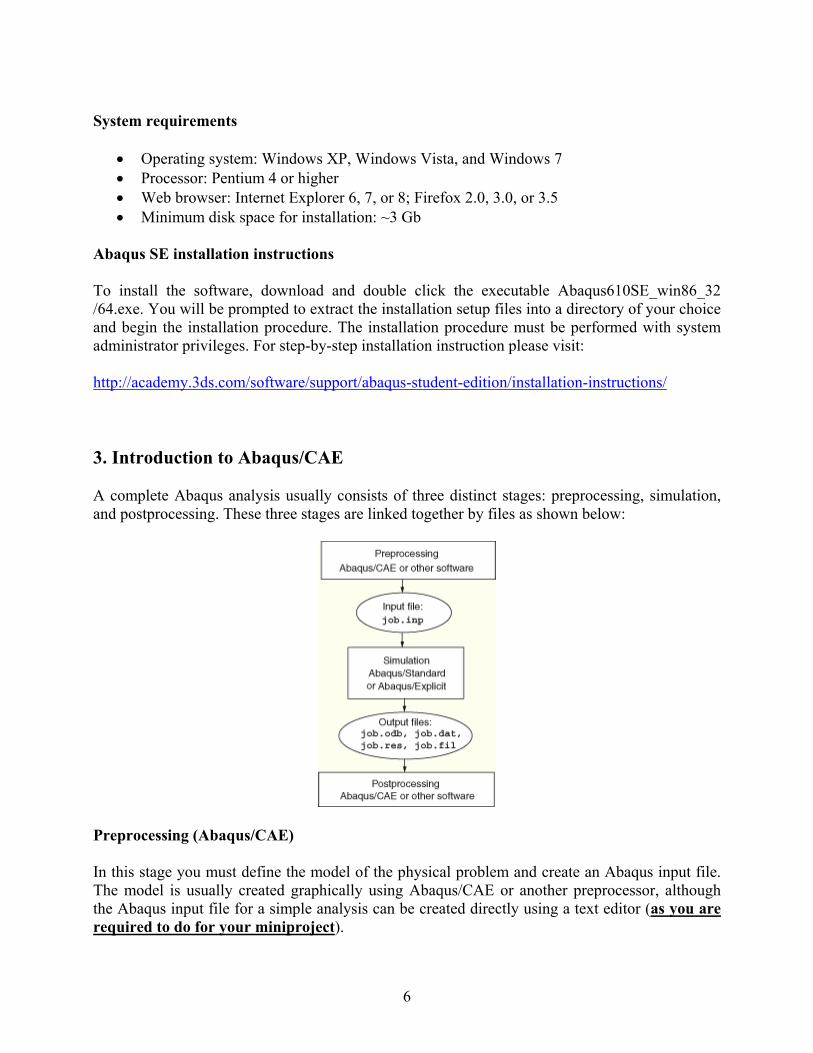
Abaqus SE installation instructions To install the software, download and double click the executable Abaqus610SE_win86_32 /64.exe. You will be prompted to extract the installation setup files into a directory of your choice and begin the installation procedure. The installation procedure must be performed with system administrator privileges. For step-by-step installation instruction please visit: http://academy.3ds.com/software/support/abaqus-student-edition/installation-instructions/ 3. Introduction to Abaqus/CAE A complete Abaqus analysis usually consists of three distinct stages: preprocessing, simulation, and postprocessing. These three stages are linked together by files as shown below:

Preprocessing (Abaqus/CAE) In this stage you must define the model of the physical problem and create an Abaqus input file. The model is usually created graphically using Abaqus/CAE or another preprocessor, although the Abaqus input file for a simple analysis can be created directly using a text editor (as you are required to do for your miniproject).

7

Simulation (Abaqus /Standard or Abaqus /Explicit) The simulation, which normally is run as a background process, is the stage in which Abaqus/Standard or Abaqus/Explicit solves the numerical problem defined in the model. Examples of output from a stress analysis include displacements and stresses that are stored in binary files ready for postprocessing. Depending on the complexity of the problem being analyzed and the power of the computer being used, it may take anywhere from seconds to days to complete an analysis run. Postprocessing (Abaqus /CAE) You can evaluate the results once the simulation has been completed and the displacements, stresses, or other fundamental variables have been calculated. The evaluation is generally done interactively using the Visualization module of Abaqus/CAE or another postprocessor. The Visualization module, which reads the neutral binary output database file, has a variety of options for displaying the results, including color contour plots, animations, deformed shape plots, and X–Y plots. The Abaqus/CAE is the Complete Abaqus Environment that provides a simple, consistent interface for creating Abaqus models, interactively submitting and monitoring Abaqus jobs, and evaluating results from Abaqus simulations. Abaqus/CAE is divided into modules, where each module defines a logical aspect of the modeling process; for example, defining the geometry, defining material properties, and generating a mesh. As you move from module to module, you build up the model. When the model is complete, Abaqus/CAE generates an input file that you submit to the Abaqus analysis product. The input file may also be created manually. An example demonstrating how this is done is presented in section 4. For the course major project, you may choose to create the input file using Abaqus/CAE. To learn about Abaqus the best resource is “Getting started with Abaqus: Interactive edition” of the Abaqus SE documentation. 3.1 Starting Abaqus/CAE To start Abaqus/CAE, you click on the Start menu at your computer then chose from programs Abaqus SE then Abaqus CAE. When Abaqus/CAE begins, the Start Session dialog box appears. The following session startup options are available:

Create Model Database allows you to begin a new analysis. Open Database allows you to open a previously saved model or output database file. Run Script allows you to run a file containing Abaqus/CAE commands. Start Tutorial allows you to begin an introductory tutorial from the online

documentation. 3.2 Components of the main window

8

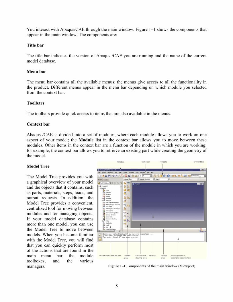
You interact with Abaqus/CAE through the main window. Figure 1–1 shows the components that appear in the main window. The components are: Title bar The title bar indicates the version of Abaqus /CAE you are running and the name of the current model database. Menu bar The menu bar contains all the available menus; the menus give access to all the functionality in the product. Different menus appear in the menu bar depending on which module you selected from the context bar. Toolbars The toolbars provide quick access to items that are also available in the menus. Context bar Abaqus /CAE is divided into a set of modules, where each module allows you to work on one aspect of your model; the Module list in the context bar allows you to move between these modules. Other items in the context bar are a function of the module in which you are working; for example, the context bar allows you to retrieve an existing part while creating the geometry of the model. Model Tree The Model Tree provides you with a graphical overview of your model and the objects that it contains, such as parts, materials, steps, loads, and output requests. In addition, the Model Tree provides a convenient, centralized tool for moving between modules and for managing objects. If your model database contains more than one model, you can use the Model Tree to move between models. When you become familiar with the Model Tree, you will find that you can quickly perform most of the actions that are found in the main menu bar, the module toolboxes, and the various managers.

Figure 1–1 Components of the main window (Viewport)

9

Results Tree The Results Tree provides you with a graphical overview of your output databases and other session-specific data such as X–Y plots. If you have more than one output database open in your session, you can use the Results Tree to move between output databases. When you become familiar with the Results Tree, you will find that you can quickly perform most of the actions in the Visualization module that are found in the main menu bar and the toolbox.. Toolbox area When you enter a module, the toolbox area displays tools in the toolbox that are appropriate for that module. The toolbox allows quick access to many of the module functions that are also available from the menu bar. Canvas and drawing area The canvas can be thought of as an infinite screen or bulletin board on which you post viewports. The drawing area is the visible portion of the canvas. Viewport Viewports are windows on the canvas in which Abaqus /CAE displays your model. Prompt area The prompt area displays instructions for you to follow during a procedure; for example, it asks you to select the geometry as you create a set. Message area Abaqus/CAE prints status information and warnings in the message area. To resize the message area, drag the top edge; to see information that has scrolled out of the message area, use the scroll bar on the right side. The message area is displayed by default, but it uses the same space occupied by the command line interface. If you have recently used the command line interface,

you must click the tab in the bottom left corner of the main window to activate the message area. Note: If new messages are added while the command line interface is active, Abaqus /CAE changes the background color surrounding the message area icon to red. When you display the message area, the background reverts to its normal color. Command line interface You can use the command line interface to type Python commands and evaluate mathematical expressions using the Python interpreter that is built into Abaqus /CAE. The interface includes primary (>>>) and secondary (...) prompts to indicate when you must indent commands to comply with Python syntax.

10

The command line interface is hidden by default, but it uses the same space occupied by the

message area. Click the tab in the bottom left corner of the main window to switch from the

message area to the command line interface. Click the tab to return to the message area. A completed model contains everything that Abaqus needs to start the analysis. Abaqus /CAE uses a model database to store your models. When you start Abaqus /CAE, the Start Session dialog box allows you to create a new, empty model database in memory. After you start Abaqus /CAE, you can save your model database to a disk by selecting File→Save from the main menu bar; to retrieve a model database from a disk, select File→Open. 3.3 Starting Abaqus command To start Abaqus command go to Start menu then Programs→Abaqus 6.10 Student Edition→Abaqus Command, a command prompt will appear. You have to go to the folder where you have the input files. The default working directory in Abaqus is C:\Temp or C:\TemABQ, unless chosen other working directory.

11

Instructions for Miniproject : Trusses

12

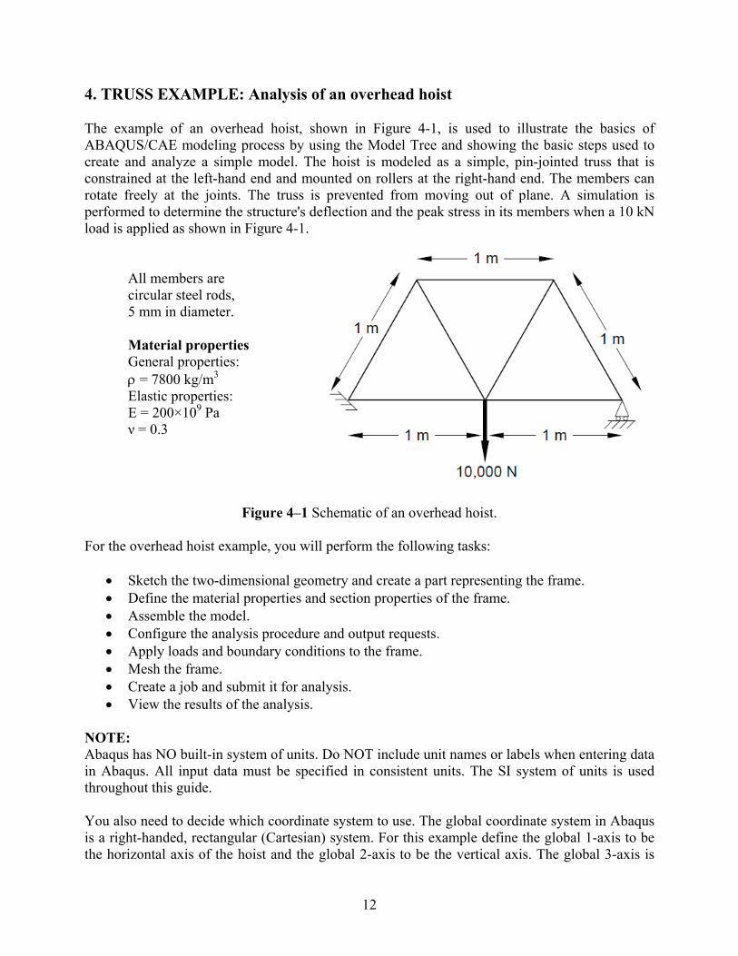
4. TRUSS EXAMPLE: Analysis of an overhead hoist The example of an overhead hoist, shown in Figure 4-1, is used to illustrate the basics of ABAQUS/CAE modeling process by using the Model Tree and showing the basic steps used to create and analyze a simple model. The hoist is modeled as a simple, pin-jointed truss that is constrained at the left-hand end and mounted on rollers at the right-hand end. The members can rotate freely at the joints. The truss is prevented from moving out of plane. A simulation is performed to determine the structure's deflection and the peak stress in its members when a 10 kN load is applied as shown in Figure 4-1.

All members are circular steel rods, 5 mm in diameter. Material properties General properties: = 7800 kg/m3 Elastic properties: E = 200×109 Pa ν = 0.3

Figure 4–1 Schematic of an overhead hoist.

For the overhead hoist example, you will perform the following tasks:

Sketch the two-dimensional geometry and create a part representing the frame. Define the material properties and section properties of the frame. Assemble the model. Configure the analysis procedure and output requests. Apply loads and boundary conditions to the frame. Mesh the frame. Create a job and submit it for analysis. View the results of the analysis.

NOTE: Abaqus has NO built-in system of units. Do NOT include unit names or labels when entering data in Abaqus. All input data must be specified in consistent units. The SI system of units is used throughout this guide. You also need to decide which coordinate system to use. The global coordinate system in Abaqus is a right-handed, rectangular (Cartesian) system. For this example define the global 1-axis to be the horizontal axis of the hoist and the global 2-axis to be the vertical axis. The global 3-axis is

13

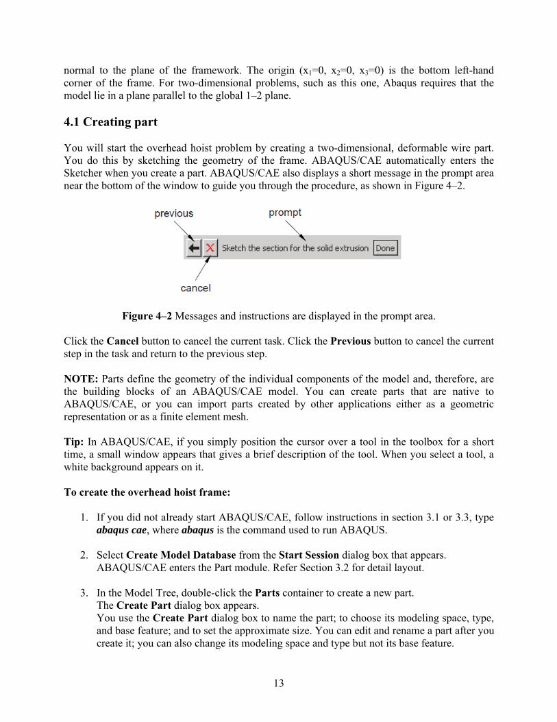
normal to the plane of the framework. The origin (x1=0, x2=0, x3=0) is the bottom left-hand corner of the frame. For two-dimensional problems, such as this one, Abaqus requires that the model lie in a plane parallel to the global 1–2 plane. 4.1 Creating part You will start the overhead hoist problem by creating a two-dimensional, deformable wire part. You do this by sketching the geometry of the frame. ABAQUS/CAE automatically enters the Sketcher when you create a part. ABAQUS/CAE also displays a short message in the prompt area near the bottom of the window to guide you through the procedure, as shown in Figure 4–2.

Figure 4–2 Messages and instructions are displayed in the prompt area. Click the Cancel button to cancel the current task. Click the Previous button to cancel the current step in the task and return to the previous step. NOTE: Parts define the geometry of the individual components of the model and, therefore, are the building blocks of an ABAQUS/CAE model. You can create parts that are native to ABAQUS/CAE, or you can import parts created by other applications either as a geometric representation or as a finite element mesh. Tip: In ABAQUS/CAE, if you simply position the cursor over a tool in the toolbox for a short time, a small window appears that gives a brief description of the tool. When you select a tool, a white background appears on it. To create the overhead hoist frame:

1. If you did not already start ABAQUS/CAE, follow instructions in section 3.1 or 3.3, type abaqus cae, where abaqus is the command used to run ABAQUS.

2. Select Create Model Database from the Start Session dialog box that appears. ABAQUS/CAE enters the Part module. Refer Section 3.2 for detail layout.

3. In the Model Tree, double-click the Parts container to create a new part. The Create Part dialog box appears. You use the Create Part dialog box to name the part; to choose its modeling space, type, and base feature; and to set the approximate size. You can edit and rename a part after you create it; you can also change its modeling space and type but not its base feature.

14

4. Name the part Frame. Choose a two-dimensional planar deformable body and a wire base

feature.

5. In the Approximate size text field, type 4.0. The value entered in the Approximate size text field at the bottom of the dialog box sets the approximate size of the new part.

6. Click Continue to exit the Create Part dialog box. ABAQUS/CAE automatically enters the Sketcher. The Sketcher toolbox appears in the left side of the main window, and the Sketcher grid appears in the viewport. The Sketcher contains a set of basic tools that allow you to sketch the two-dimensional profile of your part. ABAQUS/CAE enters the Sketcher whenever you create or edit a part. To finish using any tool, click mouse button 2 in the viewport or select a new tool. The following aspects of the Sketcher help you sketch the desired geometry:

The Sketcher grid helps you position the cursor and align objects in the viewport. Dashed lines indicate the X- and Y-axes of the sketch and intersect at the origin of

the sketch. A triad in the lower-left corner of the viewport indicates the relationship between

the sketch plane and the orientation of the part. When you select a sketching tool, ABAQUS/CAE displays the X- and Y-

coordinates of the cursor in the upper-left corner of the viewport.

7. Use the Create Isolated Point tool located in the upper left corner of the Sketcher toolbox to begin sketching the geometry of the frame by defining isolated points. Create three points with the following coordinates: (-1.0, 0.0), (0.0, 0.0), and (1.0, 0.0). The positions of these points represent the locations of the joints on the bottom of the frame.

Reset the view using the Auto-Fit View tool in the toolbar to see the three points. Click mouse button 2 anywhere in the viewport to exit the isolated point tool.

8. The positions of the points on the top of the frame are not obvious but can be easily determined by making use of the fact that the frame members form 60° angles with each other. In this case construction geometry can be used to determine the positions of these points. You create construction geometry in the Sketcher to help you position and align the geometry in your sketch. The Sketcher allows you to add construction lines and circles to your sketch; in addition, isolated points can be considered construction geometry. For more information on construction geometry, see “Creating construction geometry”, Section 19.10 of the ABAQUS/CAE User’s Manual.

8.1 Use the Create Construction: Line at an Angle tool to create angular construction lines through each of the points created in Step 8. To select the angular construction line tool, do the following:

15

8.1.1 Note the small black triangles at the base of some of the toolbox icons. These triangles indicate the presence of hidden icons that can be revealed.

Click the Create Construction: Horizontal Line Thru Point tool located on the middle-left of the Sketcher toolbox, but do not release mouse button 1. Additional icons appear.

8.1.2 Without releasing mouse button 1, drag the cursor along the set of icons that appear until you reach the angular construction line tool. Then release the mouse button to select that tool.

The angular construction line drawing tool appears in the Sketcher toolbox with a white background indicating that you selected it.

8.2 Enter 60.0 in the prompt area as the angle the construction line will make with the horizontal.

8.3 Place the cursor at the point whose coordinates are (−1.0, 0.0), and click mouse button 1 to create the construction line.

9. Similarly, create construction lines through the other two points created in Step 8.

9.1 Create another angular construction line oriented 60° with respect to the horizontal

through the point whose coordinates are (0.0, 0.0).

9.2 Create two angular construction lines oriented 120° with respect to the horizontal through the points (0.0, 0.0) and (1.0, 0.0). (You will have to exit the drawing tool by clicking mouse button 2 in the viewport and then reselect the tool to enter another angle value.)

The sketch with the isolated points and construction lines is shown in Figure 4–3. In

this figure the Sketcher Options tool has been used to suppress the visibility of every other grid line.

10. If you make a mistake while using the Sketcher, you can delete lines in your sketch, as explained in the following procedure:

10.1 From the Sketcher toolbox, click the Delete Entities tool . 10.2 In the sketch, click on a line to select it. ABAQUS/CAE highlights the selected

line in red.

10.3 Click mouse button 2 in the viewport to delete the selected line.

10.4 Repeat Steps 10.2 and 10.3 as often as necessary.

16

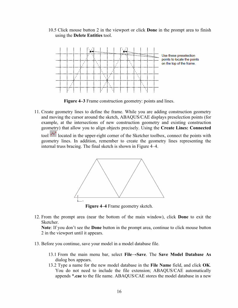
10.5 Click mouse button 2 in the viewport or click Done in the prompt area to finish using the Delete Entities tool.

Figure 4–3 Frame construction geometry: points and lines.

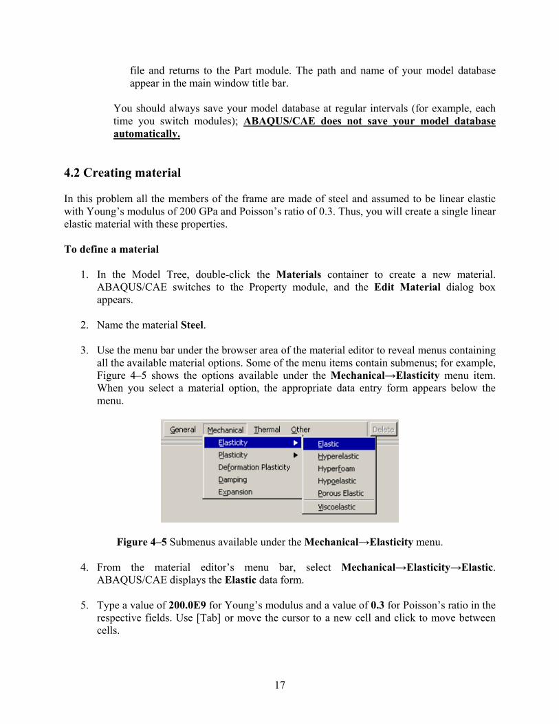
11. Create geometry lines to define the frame. While you are adding construction geometry and moving the cursor around the sketch, ABAQUS/CAE displays preselection points (for example, at the intersections of new construction geometry and existing construction geometry) that allow you to align objects precisely. Using the Create Lines: Connected

tool located in the upper-right corner of the Sketcher toolbox, connect the points with geometry lines. In addition, remember to create the geometry lines representing the internal truss bracing. The final sketch is shown in Figure 4–4.

Figure 4–4 Frame geometry sketch.

12. From the prompt area (near the bottom of the main window), click Done to exit the

Sketcher. Note: If you don’t see the Done button in the prompt area, continue to click mouse button 2 in the viewport until it appears.

13. Before you continue, save your model in a model database file.

13.1 From the main menu bar, select File→Save. The Save Model Database As dialog box appears.

13.2 Type a name for the new model database in the File Name field, and click OK. You do not need to include the file extension; ABAQUS/CAE automatically appends *.cae to the file name. ABAQUS/CAE stores the model database in a new

17

file and returns to the Part module. The path and name of your model database appear in the main window title bar.

You should always save your model database at regular intervals (for example, each time you switch modules); ABAQUS/CAE does not save your model database automatically.

4.2 Creating material In this problem all the members of the frame are made of steel and assumed to be linear elastic with Young’s modulus of 200 GPa and Poisson’s ratio of 0.3. Thus, you will create a single linear elastic material with these properties. To define a material

1. In the Model Tree, double-click the Materials container to create a new material. ABAQUS/CAE switches to the Property module, and the Edit Material dialog box appears.

2. Name the material Steel.

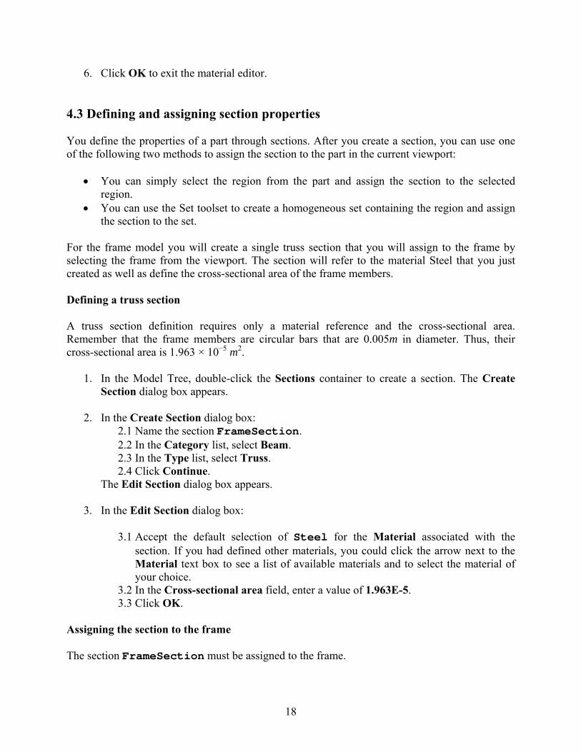
3. Use the menu bar under the browser area of the material editor to reveal menus containing all the available material options. Some of the menu items contain submenus; for example, Figure 4–5 shows the options available under the Mechanical→Elasticity menu item. When you select a material option, the appropriate data entry form appears below the menu.

Figure 4–5 Submenus available under the Mechanical→Elasticity menu.

4. From the material editor’s menu bar, select Mechanical→Elasticity→Elastic. ABAQUS/CAE displays the Elastic data form.

5. Type a value of 200.0E9 for Young’s modulus and a value of 0.3 for Poisson’s ratio in the respective fields. Use [Tab] or move the cursor to a new cell and click to move between cells.

18

6. Click OK to exit the material editor. 4.3 Defining and assigning section properties You define the properties of a part through sections. After you create a section, you can use one of the following two methods to assign the section to the part in the current viewport:

You can simply select the region from the part and assign the section to the selected

region. You can use the Set toolset to create a homogeneous set containing the region and assign

the section to the set.

For the frame model you will create a single truss section that you will assign to the frame by selecting the frame from the viewport. The section will refer to the material Steel that you just created as well as define the cross-sectional area of the frame members. Defining a truss section A truss section definition requires only a material reference and the cross-sectional area. Remember that the frame members are circular bars that are 0.005m in diameter. Thus, their cross-sectional area is 1.963 × 10−5 m2.

1. In the Model Tree, double-click the Sections container to create a section. The Create Section dialog box appears.

2. In the Create Section dialog box: 2.1 Name the section FrameSection. 2.2 In the Category list, select Beam. 2.3 In the Type list, select Truss. 2.4 Click Continue.

The Edit Section dialog box appears.

3. In the Edit Section dialog box:

3.1 Accept the default selection of Steel for the Material associated with the section. If you had defined other materials, you could click the arrow next to the Material text box to see a list of available materials and to select the material of your choice.

3.2 In the Cross-sectional area field, enter a value of 1.963E-5. 3.3 Click OK.

Assigning the section to the frame The section FrameSection must be assigned to the frame.

19

1. In the Model Tree, expand the branch for the part named Frame by clicking the “+” symbol to expand the Parts container and then clicking the “+” symbol to expand the Frame item.

2. Double-click Section Assignments in the list of part attributes that appears. ABAQUS/CAE displays prompts in the prompt area to guide you through the procedure.

3. Select the entire part as the region to which the section will be applied.

3.1 Click and hold mouse button 1 at the upper left-hand corner of the viewport. 3.2 Drag the mouse to create a box around the truss. 3.3 Release mouse button 1.

ABAQUS/CAE highlights the entire frame.

4. Click mouse button 2 in the viewport or click Done in the prompt area to accept the selected geometry. The Edit Section Assignment dialog box appears containing a list of existing sections.

5. Accept the default selection of FrameSection, and click OK. ABAQUS/CAE assigns the truss section to the frame, colors the entire frame aqua to indicate that the region has a section assignment, and closes the Edit Section Assignment dialog box.

4.4 Defining the assembly Each part that you create is oriented in its own coordinate system and is independent of the other parts in the model. Although a model may contain many parts, it contains only one assembly. You define the geometry of the assembly by creating instances of a part and then positioning the instances relative to each other in a global coordinate system. An instance may be independent or dependent. Independent part instances are meshed individually, while the mesh of a dependent part instance is associated with the mesh of the original part. For further details, see “Working with part instances,” Section 13.3 of the ABAQUS/CAE User’s Manual. By default, part instances are dependent. For this problem you will create a single instance of your overhead hoist. ABAQUS/CAE positions the instance so that the origin of the sketch that defined the frame overlays the origin of the assembly’s default coordinate system. To define the assembly

1. In the Model Tree, expand the Assembly container and double-click Instances in the list that appears. ABAQUS/CAE switches to the Assembly module, and the Create Instance dialog box appears.

2. In the dialog box, select Frame and click OK.

20

ABAQUS/CAE creates an instance of the overhead hoist. In this example the single instance of the frame defines the assembly. The frame is displayed in the 1–2 plane of the global coordinate system (a right-handed, rectangular Cartesian system). A triad in the lower-left corner of the viewport indicates the orientation of the model with respect to the view. A second triad in the viewport indicates the origin and orientation of the global coordinate system (X-, Y-, and Z-axes). The global 1-axis is the horizontal axis of the hoist, the global 2-axis is the vertical axis, and the global 3-axis is normal to the plane of the framework. For two-dimensional problems such as this one ABAQUS requires that the model lie in a plane parallel to the global 1–2 plane. 4.5 Configuring analysis Now that you have created your assembly, you can configure your analysis. In this simulation we are interested in the static response of the overhead hoist to a 10 kN load applied at the center, with the left-hand end fully constrained and a roller constraint on the right-hand end (see Figure 4–1). This is a single event, so only a single analysis step is needed for the simulation. Thus, the analysis will consist of two steps overall:

An initial step, in which you will apply boundary conditions that constrain the ends of the

frame. An analysis step, in which you will apply a concentrated load at the center of the frame.

ABAQUS/CAE generates the initial step automatically, but you must create the analysis step yourself. You may also request output for any steps in the analysis. There are two kinds of analysis steps in ABAQUS: general analysis steps, which can be used to analyze linear or nonlinear response, and linear perturbation steps, which can be used only to analyze linear problems. Only general analysis steps are available in ABAQUS/Explicit. For this simulation you will define a static linear perturbation step. Perturbation procedures are discussed further in Chapter 11, “Multiple Step Analysis.” Creating a static linear perturbation analysis step Create a static, linear perturbation step that follows the initial step of the analysis.

1. In the Model Tree, double-click the Steps container to create a step.

ABAQUS/CAE switches to the Step module, and the Create Step dialog box appears. A list of all the general procedures and a default step name of Step-1 is provided.

2. Change the step name to Apply load. 3. Select Linear perturbation as the Procedure type. 4. From the list of available linear perturbation procedures in the Create Step dialog box,

select Static, Linear perturbation and click Continue. The Edit Step dialog box appears with the default settings for a static linear perturbation step.

21

5. The Basic tab is selected by default. In the Description field, type 10 kN central load.

6. Click the Other tab to see its contents; you can accept the default values provided for the step.

7. Click OK to create the step and to exit the Edit Step dialog box. Requesting data output Finite element analyses can create very large amounts of output. ABAQUS allows you to control and manage this output so that only data required to interpret the results of your simulation are produced. Four types of output are available from an ABAQUS analysis:

Results stored in a neutral binary file used by ABAQUS/CAE for postprocessing. This file is called the ABAQUS output database file and has the extension *.odb.

Printed tables of results, written to the ABAQUS data (*.dat) file. Output to the data file is available only in ABAQUS/Standard.

Restart data used to continue the analysis, written to the ABAQUS restart (*.res) file. Results stored in binary files for subsequent postprocessing with third-party software,

written to the ABAQUS results (*.fil) file. You will use only the first of these in the overhead hoist simulation. A detailed discussion of printed output to the data (*.dat) file is found in “Output to the data and results files,” Section 4.1.2 of the ABAQUS Analysis User’s Manual. By default, ABAQUS/CAE writes the results of the analysis to the output database (*.odb) file. When you create a step, ABAQUS/CAE generates a default output request for the step. A list of the preselected variables written by default to the output database is given in the ABAQUS Analysis User’s Manual. You do not need to do anything to accept these defaults. You use the Field Output Requests Manager to request output of variables that should be written at relatively low frequencies to the output database from the entire model or from a large portion of the model. You use the History Output Requests Manager to request output of variables that should be written to the output database at a high frequency from a small portion of the model; for example, the displacement of a single node. For this example you will examine the output requests to the *.odb file and accept the default configuration. To examine your output requests to the *.odb file

1. In the Model Tree, click mouse button 3 on the Field Output Requests container and select Manager from the menu that appears. ABAQUS/CAE displays the Field Output Requests Manager. This manager displays an alphabetical list of existing output requests along the left side of the dialog box. The names of all the steps in the analysis appear along the top of the dialog box in the order of

22

execution. The table formed by these two lists displays the status of each output request in each step. You can use the Field Output Requests Manager to do the following:

Select the variables that ABAQUS will write to the output database. Select the section points for which ABAQUS will generate output data. Select the region of the model for which ABAQUS will generate output data. Change the frequency at which ABAQUS will write data to the output database.

2. Review the default output request that ABAQUS/CAE generates for the Static, Linear

perturbation step you created and named Apply load. Click the cell in the table labeled Created; that cell becomes highlighted. The following information related to the cell is shown in the legend at the bottom of the manager:

The type of analysis procedure carried out in the step in that column. The list of output request variables. The output request status.

3. On the right side of the Field Output Requests Manager, click Edit to view more

detailed information about the output request. The field output editor appears. In the Output Variables region of this dialog box, there is a text box that lists all variables that will be output. If you change an output request, you can always return to the default settings by clicking Preselected defaults above the text box.

4. Click the arrows next to each output variable category to see exactly which variables will be output. The boxes next to each category title allow you to see at a glance whether all variables in that category will be output. A black check mark indicates that all variables are output, while a gray check mark indicates that only some variables will be output. Based on the selections shown at the bottom of the dialog box, data will be generated at every default section point in the model and will be written to the output database after every increment during the analysis.

5. Click Cancel to close the field output editor, since you do not wish to make any changes to the default output requests.

6. Click Dismiss to close the Field Output Requests Manager.

7. Review the history output requests in a similar manner by right-clicking the History Output Requests container in the Model Tree and opening the history output editor.

23

4.6 Applying boundary conditions and loads to the model Prescribed conditions, such as loads and boundary conditions, are step dependent, which means that you must specify the step or steps in which they become active. Now that you have defined the steps in the analysis, you can define prescribed conditions. Applying boundary conditions to the frame In structural analyses, boundary conditions are applied to those regions of the model where the displacements and/or rotations are known. Such regions may be constrained to remain fixed (have zero displacement and/or rotation) during the simulation or may have specified, nonzero displacements and/or rotations. In this model the bottom-left portion of the frame is constrained completely and, thus, cannot move in any direction. The bottom-right portion of the frame, however, is fixed in the vertical direction but is free to move in the horizontal direction. The directions in which motion is possible are called degrees of freedom (dof). To apply boundary conditions to the frame

1. In the Model Tree, double-click the BCs container. ABAQUS/CAE switches to the Load module, and the Create Boundary Condition dialog box appears.

2. In the Create Boundary Condition dialog box: 2.1 Name the boundary condition Fixed. 2.2 From the list of steps, select Initial as the step in which the boundary condition

will be activated. All the mechanical boundary conditions specified in the Initial step must have zero magnitudes. This condition is enforced automatically by ABAQUS/CAE.

2.3 In the Category list, accept Mechanical as the default category selection. 2.4 In the Types for Selected Step list, select Displacement/Rotation, and click

Continue. ABAQUS/CAE displays prompts in the prompt area to guide you through the procedure. For example, you are asked to select the region to which the boundary condition will be applied. To apply a prescribed condition to a region, you can either select the region directly in the viewport or apply the condition to an existing set (a set is a named region of a model). Sets are a convenient tool that can be used to manage large complicated models. In this simple model you will not make use of sets.

3. In the viewport, select the vertex at the bottom-left corner of the frame as the region to

which the boundary condition will be applied.

4. Click mouse button 2 in the viewport or click Done in the prompt area to indicate that you have finished selecting regions. The Edit Boundary Condition dialog box appears. When you are defining a boundary condition in the initial step, all available degrees of freedom are unconstrained by default.

24

5. In the dialog box:

5.1 Toggle on U1 and U2 since all translational degrees of freedom need to be constrained.

5.2 Click OK to create the boundary condition and to close the dialog box. ABAQUS/CAE displays two arrowheads at the vertex to indicate the constrained degrees of freedom.

6. Repeat the above procedure to constrain degree of freedom U2 at the vertex at the bottom-

right corner of the frame. Name this boundary condition Roller.

7. In the Model Tree, click mouse button 3 on the BCs container and select Manager from the menu that appears. ABAQUS/CAE displays the Boundary Condition Manager. The manager indicates that the boundary conditions are Created (activated) in the initial step and are Propagated from base state (continue to be active) in the analysis step Apply load.

8. Click Dismiss to close the Boundary Condition Manager. In this example all the constraints are in the global 1- or 2-directions. In many cases constraints are required in directions that are not aligned with the global directions. In such cases you can define a local coordinate system for boundary condition application. The skew plate example in Chapter 5, “Using Shell Elements,” demonstrates how to do this.

Applying a load to the frame Now that you have constrained the frame, you can apply a load to the bottom of the frame. In ABAQUS the term load (as in the Load module in ABAQUS/CAE) generally refers to anything that induces a change in the response of a structure from its initial state, including:

concentrated forces, pressures, nonzero boundary conditions, body loads, and temperature (with thermal expansion of the material defined).

Sometimes the term load is used to refer specifically to force-type quantities (as in the Load Manager of the Load module); for example, concentrated forces, pressures, and body loads but not boundary conditions or temperature. The intended meaning of the term should be clear from the context of the discussion. In this simulation a concentrated force of 10 kN is applied in the negative 2-direction to the bottom center of the frame; the load is applied during the linear perturbation step you created earlier. In reality there is no such thing as a concentrated, or point, load; the load will always be

25

applied over some finite area. However, if the area being loaded is small, it is an appropriate idealization to treat the load as a concentrated load. To apply a concentrated force to the frame

1. In the Model Tree, click mouse button 3 on the Loads container and select Manager from the menu that appears. The Load Manager appears.

2. At the bottom of the Load Manager, click Create. The Create Load dialog box appears.

3. In the Create Load dialog box: 3.1 Name the load Force. 3.2 From the list of steps, select Apply load as the step in which the load will be

applied. 3.3 In the Category list, accept Mechanical as the default category selection. 3.4 In the Types for Selected Step list, accept the default selection of Concentrated

force. 3.5 Click Continue.

ABAQUS/CAE displays prompts in the prompt area to guide you through the procedure. You are asked to select a region to which the load will be applied. As with boundary conditions, the region to which the load will be applied can be selected either directly in the viewport or from a list of existing sets. As before, you will select the region directly in the viewport.

4. In the viewport, select the vertex at the bottom center of the frame as the region where the

load will be applied.

5. Click mouse button 2 in the viewport or click Done in the prompt area to indicate that you have finished selecting regions. The Edit Load dialog box appears.

6. In the dialog box: 6.1 Enter a magnitude of -10000.0 for CF2. 6.2 Click OK to create the load and to close the dialog box.

ABAQUS/CAE displays a downward-pointing arrow at the vertex to indicate that the load is applied in the negative 2-direction.

7. Examine the Load Manager and note that the new load is Created (activated) in the

analysis step Apply load. 8. Click Dismiss to close the Load Manager.

4.7 Meshing the model You will now generate the finite element mesh. You can choose the meshing technique that ABAQUS/CAE will use to create the mesh, the element shape, and the element type. The

26

meshing technique for one-dimensional regions (such as the ones in this example) cannot be changed, however. ABAQUS/CAE uses a number of different meshing techniques. The default meshing technique assigned to the model is indicated by the color of the model that is displayed when you enter the Mesh module; if ABAQUS/CAE displays the model in orange, it cannot be meshed without assistance from you. Assigning an ABAQUS element type In this section you will assign a particular ABAQUS element type to the model. Although you will assign the element type now, you could also wait until after the mesh has been created. Two-dimensional truss elements will be used to model the frame. These elements are chosen because truss elements, which carry only tensile and compressive axial loads, are ideal for modeling pin-jointed frameworks such as this overhead hoist. To assign an ABAQUS element type

1. In the Model Tree, expand the Frame item underneath the Parts container. Then double-click Mesh in the list that appears. ABAQUS/CAE switches to the Mesh module. The Mesh module functionality is available only through menu bar items or toolbox icons.

2. From the main menu bar, select Mesh→Element Type. 3. In the viewport, select the entire frame as the region to be assigned an element type. In the

prompt area, click Done when you are finished. The Element Type dialog box appears.

4. In the dialog box, select the following: Standard as the Element Library selection (the default). Linear as the Geometric Order (the default). Truss as the Family of elements.

5. In the lower portion of the dialog box, examine the element shape options. A brief description of the default element selection is available at the bottom of each tabbed page. Since the model is a two-dimensional truss, only two-dimensional truss element types are shown on the Line tabbed page. A description of the element type T2D2 appears at the bottom of the dialog box. ABAQUS/CAE will now associate T2D2 elements with the elements in the mesh.

6. Click OK to assign the element type and to close the dialog box. 7. In the prompt area, click Done to end the procedure. Creating the mesh Basic meshing is a two-stage operation: first you seed the edges of the part instance, and then you mesh the part instance. You select the number of seeds based on the desired element size or on the number of elements that you want along an edge, and ABAQUS/CAE places the

27

nodes of the mesh at the seeds whenever possible. For this problem you will create one element on each bar of the hoist. To seed and mesh the model

1. From the main menu bar, select Seed→Part to seed the part instance. Note: You can gain more control of the resulting mesh by seeding each edge of the part instance individually, but it is not necessary for this example. The Global Seeds dialog box appears. The dialog box displays the default element size that ABAQUS/CAE will use to seed the part instance. This default element size is based on the size of the part instance. A relatively large seed value will be used so that only one element will be created per region.

2. In the Global Seeds dialog box, specify an approximate global element size of 1.0, and click OK to create the seeds and to close the dialog box.

3. From the main menu bar, select Mesh→Part to mesh the part instance. 4. From the buttons in the prompt area, click Yes to confirm that you want to mesh the

part instance. Tip: You can display the node and element numbers within the Mesh module by selecting View→Part Display Options from the main menu bar. Toggle on Show node labels and Show element labels in the Mesh tabbed page of the Part Display Options dialog box that appears.

4.8 Creating an analysis job Now that you have configured your analysis, you will create a job that is associated with your model. To create an analysis job

1. In the Model Tree, double-click the Jobs container to create a job. ABAQUS/CAE switches to the Job module, and the Create Job dialog box appears with a list of the models in the model database. When you are finished defining your job, the Jobs container will display a list of your jobs.

2. Name the job Frame, and click Continue. The Edit Job dialog box appears.

3. In the Description field, type Two-dimensional overhead hoist frame. 4. In the Submission tabbed page, select Data check as the Job Type. Click OK to accept

all other default job settings in the job editor and to close the dialog box.

28

4.9 Checking the model Having generated the model for this simulation, you are ready to run the analysis. Unfortunately, it is possible to have errors in the model because of incorrect or missing data. You should perform a data check analysis first before running the simulation. To run a data check analysis

1. Make sure that the Job Type is set to Data check. In the Model Tree, click mouse button 3 on the job named Frame and select Submit from the menu that appears to submit your job for analysis.

2. After you submit your job, information appears next to the job name indicating the job’s status. The status of the overhead hoist problem indicates one of the following conditions:

Submitted while the job is being submitted for analysis. Running while ABAQUS analyzes the model. Completed when the analysis is complete, and the output has been written to the

output database. Aborted if ABAQUS/CAE finds a problem with the input file or the analysis and

aborts the analysis. In addition, ABAQUS/CAE reports the problem in the message area.

During the analysis, ABAQUS/Standard sends information to ABAQUS/CAE to allow you to monitor the progress of the job. Information from the status, data, log, and message files appear in the job monitor dialog box. To monitor the status of a job In the Model Tree, click mouse button 3 on the job named Frame and select Monitor from the menu that appears to open the job monitor dialog box. The top half of the dialog box displays the information available in the status (*.sta) file that ABAQUS creates for the analysis. This file contains a brief summary of the progress of an analysis and is described in “Output,” Section 4.1.1 of the ABAQUS Analysis User’s Manual. The bottom half of the dialog box displays the following information:

Click the Log tab to display the start and end times for the analysis that appear in the log (*.log) file.

Click the Errors and Warnings tabs to display the first ten errors or the first ten warnings that appear in the data (*.dat) and message (*.msg) files. If a particular region of the model is causing the error or warning, a node or element set will be created automatically that contains that region. The name of the node or element set appears with the error or warning message, and you can view the set using display groups in the Visualization module. It will not be possible to perform the analysis until the causes of any error messages are corrected. In addition, you should always investigate the reason for any warning messages

29

to determine whether corrective action is needed or whether such messages can be ignored safely. If more than ten errors or warnings are encountered, information regarding the additional errors and warnings can be obtained from the printed output files themselves.

Click the Output tab to display a record of each output data entry as it is written to the output database.

4.10 Running the analysis Make any necessary corrections to your model. When the data check analysis completes with no error messages, run the analysis itself. To do this, edit the job definition and set the Job Type to Continue analysis; then, resubmit your job for analysis. You should always perform a data check analysis before running a simulation to ensure that the model has been defined correctly and to check that there is enough disk space and memory available to complete the analysis. However, it is possible to combine the data check and analysis phases of the simulation by setting the Job Type to Full analysis. If a simulation is expected to take a substantial amount of time, it may be convenient to run it in a batch queue by selecting Queue as the Run Mode. (The availability of such a queue depends on your computer. If you have any questions, ask your systems administrator how to run ABAQUS on your system.) 4.11 Postprocessing with Abaqus/CAE Graphical postprocessing is important because of the great volume of data created during a simulation. For any realistic model it is impractical for you to try to interpret results in the tabular form of the data file. Abaqus/Viewer allows you to view the results graphically using a variety of methods, including deformed shape plots, contour plots, vector plots, animations, and X–Y plots. Start Abaqus/Viewer by going to Start menu then All Programs→Abaqus 6.10 Student Edition →Abaqus viewer. The Abaqus/Viewer window appears. To begin, open the output database file that Abaqus/Standard generated during the analysis of the problem:

1. From the main menu bar, select File→Open; or use the tool in the toolbar. The Open Database dialog box appears.

2. From the list of available output database files, select Frame.odb. 3. Click OK.

Abaqus/Viewer displays a fast plot of the model. A fast plot is a basic representation of the undeformed model shape and is an indication that you have opened the desired file. Important: The fast plot does not display results and cannot be customized, for example, to display element and node numbers. You must display the undeformed model shape to customize the appearance of the model.

30

The title block at the bottom of the viewport indicates the following:

The description of the model (from the first line of the *HEADING option in the input file).

The name of the output database (from the name of the analysis job). The product name (Abaqus/Standard or Abaqus/Explicit) and version used to generate the

output database. The date the output database was last modified.

The state block at the bottom of the viewport indicates the following:

Which step is being displayed. The increment within the step. The step time.

The view orientation triad indicates the orientation of the model in the global coordinate system. You will now display the undeformed model shape and use the plot options to enable the display of node and element numbering in the plot. From the main menu bar, select Plot→Undeformed

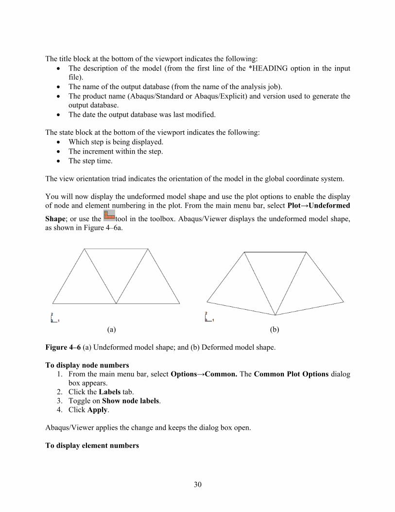
Shape; or use the tool in the toolbox. Abaqus/Viewer displays the undeformed model shape, as shown in Figure 4–6a.

(a) (b) Figure 4–6 (a) Undeformed model shape; and (b) Deformed model shape. To display node numbers

1. From the main menu bar, select Options→Common. The Common Plot Options dialog box appears.

2. Click the Labels tab. 3. Toggle on Show node labels. 4. Click Apply.

Abaqus/Viewer applies the change and keeps the dialog box open. To display element numbers

31

1. In the Labels tabbed page of the Undeformed Shape Plot Options dialog box, toggle on Show element labels.

2. Click OK. Abaqus/Viewer applies the change and closes the dialog box. To disable the display of node and element numbers in the undeformed shape plot, repeat the above procedure and, under Labels, toggle off Show node labels and Show element labels. You will now display the deformed model shape and use the plot options to change the deformation scale factor and overlay the undeformed model shape on the deformed model shape.

From the main menu bar, select Plot→Deformed Shape; or use the tool in the toolbox. Abaqus/Viewer displays the deformed model shape, as shown in Figure 4–6b. For small-displacement analyses the displacements are scaled automatically to ensure that they are clearly visible. The scale factor is displayed in the state block. In this case the displacements have been scaled by a factor of 42.83. To change the deformation scale factor

1. From the main menu bar, select Options→Common. 2. From the Common Plot Options dialog box, click the Basic tab if it is not already

selected. 3. From the Deformation Scale Factor area, toggle on Uniform and enter 10.0 in the Value

field. 4. Click Apply to redisplay the deformed shape.

The state block displays the new scale factor. To return to automatic scaling of the displacements, repeat the above procedure and, in the Deformation Scale Factor field, toggle on Auto-compute. To overlay the undeformed model shape on the deformed model shape:

1. Click the tool in the toolbox to allow multiple plot states in the viewport; then click the

tool or select Plot→Undeformed Shape to add the undeformed shape plot to the existing deformed plot in the viewport. By default, Abaqus/CAE plots the deformed model shape in green and the (superimposed) undeformed model shape in a translucent white.

2. The plot options for the superimposed image are controlled separately from those of the

primary image. From the main menu bar, select Options→Superimpose; or use the tool in the toolbox to change the edge style of the superimposed (i.e., undeformed) image.

3. From the Superimpose Plot Options dialog box, click the Color & Style tab. 4. In the Color & Style tabbed page, select the dashed edge style. 5. Click OK to close the Superimpose Plot Options dialog box and to apply the change.

The boundary conditions applied to the overhead hoist model can also be displayed and checked using Abaqus/Viewer:

32

1. From the main menu bar, select Plot→Undeformed Shape; or use the tool in the toolbox.

2. From the main menu bar, select View→ODB Display Options. 3. In the ODB Display Options dialog box, click the Entity Display tab. 4. Toggle on Show boundary conditions. 5. Click OK.

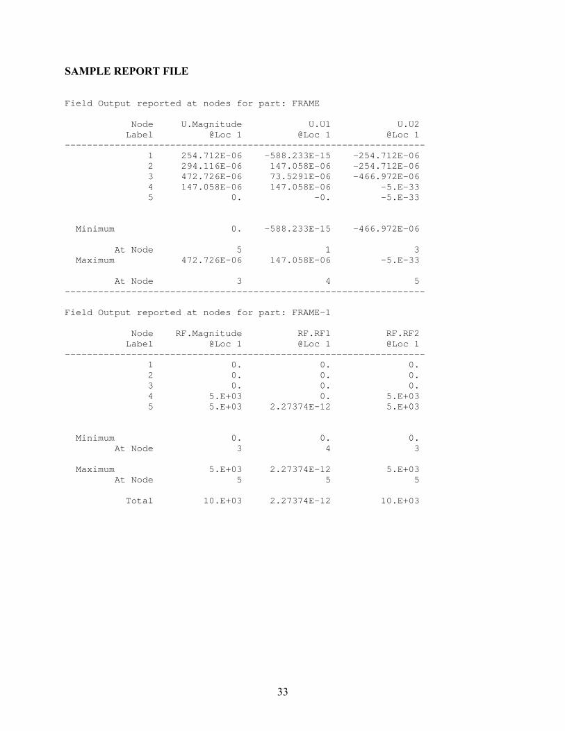
Abaqus/Viewer displays symbols to indicate the applied boundary conditions. Tabular data reports In addition to the graphical capabilities described above, Abaqus/CAE allows you to write data to a text file in a tabular format. As you have already noticed, if you included what you needed to report in the .inp file, then you would get a corresponding report in the truss.dat file. However, you may want the report after you have performed simulation. In this case, the reporting facility is a convenient alternative to writing tabular output to the data (*.dat) file. Output generated this way has many uses; for example, it can be used in written reports. In this problem you will generate a report containing the element stresses, nodal displacements, and reaction forces. To generate field data reports

1. From the main menu bar, select Report→Field Output. 2. In the Variable tabbed page of the Report Field Output dialog box, accept the default

position labeled Integration Point. Click the triangle next to S: Stress components to expand the list of available variables. From this list, toggle on S11.

3. In the Setup tabbed page, name the report Frame.rpt. In the Data region at the bottom of the page, toggle off Column totals.

4. Click Apply. The element stresses are written to the report file.

5. In the Variable tabbed page of the Report Field Output dialog box, change the position to Unique Nodal. Toggle off S: Stress components, and select U1 and U2 from the list of available U: Spatial displacement variables.

6. Click Apply. The nodal displacements are appended to the report file.

7. In the Variable tabbed page of the Report Field Output dialog box, toggle off U: Spatial displacement, and select RF1 and RF2 from the list of available RF: Reaction force variables.

8. In the Data region at the bottom of the Setup tabbed page, toggle on Column totals. 9. Click OK.

The reaction forces are appended to the report file, and the Report Field Output dialog box closes

Exiting Abaqus/Viewer From the main menu bar, select File→Exit to exit Abaqus/Viewer.

33

SAMPLE REPORT FILE Field Output reported at nodes for part: FRAME Node U.Magnitude U.U1 U.U2 Label @Loc 1 @Loc 1 @Loc 1 ----------------------------------------------------------------- 1 254.712E-06 -588.233E-15 -254.712E-06 2 294.116E-06 147.058E-06 -254.712E-06 3 472.726E-06 73.5291E-06 -466.972E-06 4 147.058E-06 147.058E-06 -5.E-33 5 0. -0. -5.E-33 Minimum 0. -588.233E-15 -466.972E-06 At Node 5 1 3 Maximum 472.726E-06 147.058E-06 -5.E-33 At Node 3 4 5 ----------------------------------------------------------------- Field Output reported at nodes for part: FRAME-1 Node RF.Magnitude RF.RF1 RF.RF2 Label @Loc 1 @Loc 1 @Loc 1 ----------------------------------------------------------------- 1 0. 0. 0. 2 0. 0. 0. 3 0. 0. 0. 4 5.E+03 0. 5.E+03 5 5.E+03 2.27374E-12 5.E+03 Minimum 0. 0. 0. At Node 3 4 3 Maximum 5.E+03 2.27374E-12 5.E+03 At Node 5 5 5 Total 10.E+03 2.27374E-12 10.E+03

34

2D/3D problems

35

Pressure= 10kN/m2

y

x

1cm

10 cm

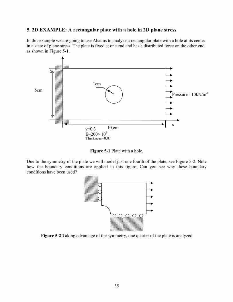
5. 2D EXAMPLE: A rectangular plate with a hole in 2D plane stress In this example we are going to use Abaqus to analyze a rectangular plate with a hole at its center in a state of plane stress. The plate is fixed at one end and has a distributed force on the other end as shown in Figure 5-1.

Figure 5-1 Plate with a hole. Due to the symmetry of the plate we will model just one fourth of the plate, see Figure 5-2. Note how the boundary conditions are applied in this figure. Can you see why these boundary conditions have been used?

Figure 5-2 Taking advantage of the symmetry, one quarter of the plate is analyzed

5cm

ν=0.3 E=200109

Thickness=0.01

36

5.1 Creating a part Start Abaqus/CAE form programs in the Start menu. 1. Select Create Model Database from the Start Session dialog box that appears. When the

Part module has finished loading, it displays the Part module toolbox in the left side of the Abaqus/CAE main window. Each module displays its own set of tools in the module toolbox.

2. From the main menu bar, select Part→Create to create a new part. The Create Part dialog box appears. You use the Create Part dialog box to name the part; to choose its modeling space, type, and base feature; and to set the approximate size. You can edit and rename a part after you create it, but you cannot change its modeling space, type, or base feature.

3. Name the part Plate. Choose a two-dimensional planar deformable body and a shell base feature.

4. In the Approximate size text field, type 20. 5. Click Continue to exit the Create Part dialog box.

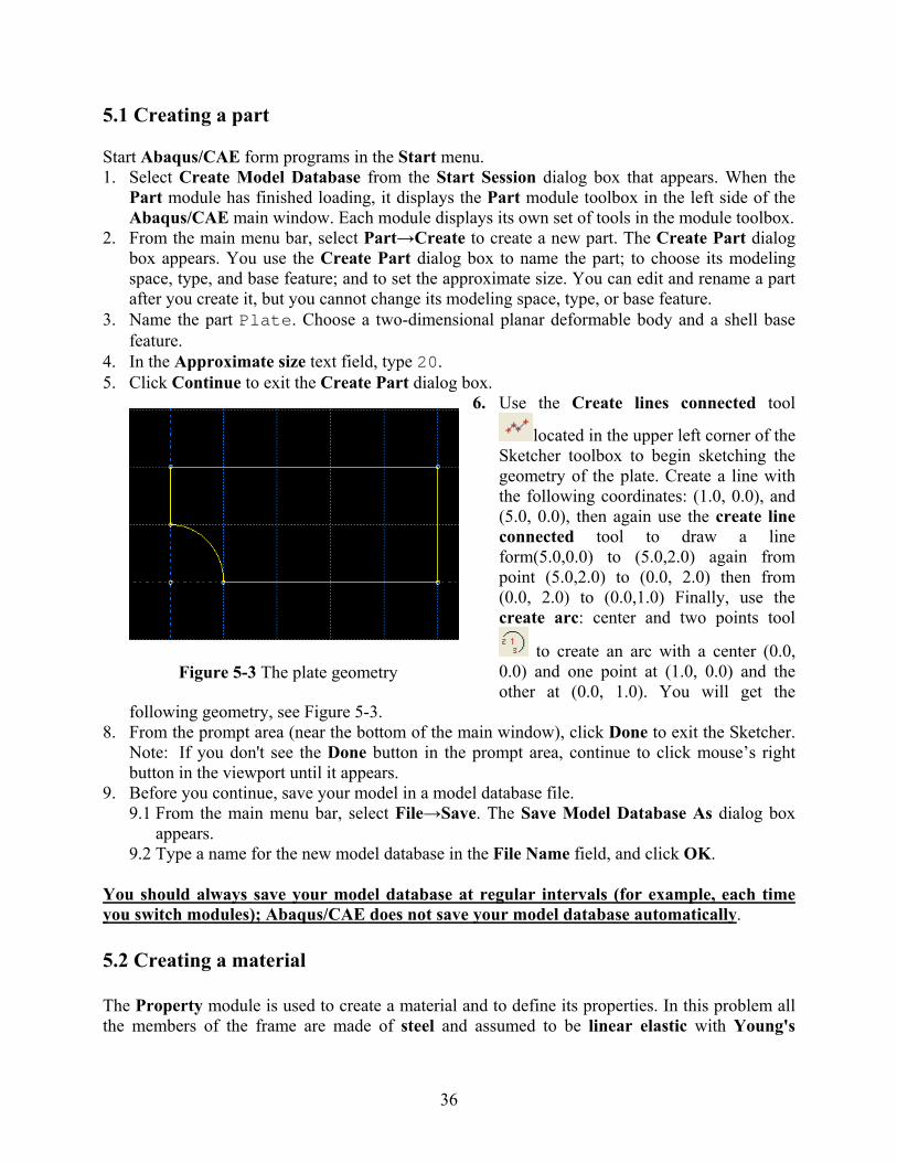
6. Use the Create lines connected tool

located in the upper left corner of the Sketcher toolbox to begin sketching the geometry of the plate. Create a line with the following coordinates: (1.0, 0.0), and (5.0, 0.0), then again use the create line connected tool to draw a line form(5.0,0.0) to (5.0,2.0) again from point (5.0,2.0) to (0.0, 2.0) then from (0.0, 2.0) to (0.0,1.0) Finally, use the create arc: center and two points tool

to create an arc with a center (0.0, 0.0) and one point at (1.0, 0.0) and the other at (0.0, 1.0). You will get the

following geometry, see Figure 5-3. 8. From the prompt area (near the bottom of the main window), click Done to exit the Sketcher.

Note: If you don't see the Done button in the prompt area, continue to click mouse’s right button in the viewport until it appears.

9. Before you continue, save your model in a model database file. 9.1 From the main menu bar, select File→Save. The Save Model Database As dialog box

appears. 9.2 Type a name for the new model database in the File Name field, and click OK.

You should always save your model database at regular intervals (for example, each time you switch modules); Abaqus/CAE does not save your model database automatically. 5.2 Creating a material The Property module is used to create a material and to define its properties. In this problem all the members of the frame are made of steel and assumed to be linear elastic with Young's

Figure 5-3 The plate geometry

37

modulus of 200 GPa and Poisson's ratio of 0.3. Thus, you will create a single linear elastic material with these properties. To define a material: 1. In the Module list located under the toolbar, select Property to enter the Property module.

The cursor changes to an hourglass while the Property module loads. 2. From the main menu bar, select Material→Create to create a new material. The Edit

Material dialog box appears. 3. Name the material Steel. 4. From the material editor's menu bar, select Mechanical→Elasticity→Elastic. Abaqus/CAE

displays the Elastic data form. 5. Type a value of 200.0E9 for Young's modulus and a value of 0.3 for Poisson's ratio in the

respective fields. Use [Tab] or move the cursor to a new cell and click to move between cells. 6. Click OK to exit the material editor. 7. Now Save. 5.3 Defining and assigning section properties The section properties of a model is defined by creating sections in the Property module. After the section is created, one of the following two methods to assign the section to the part in the current viewport can be used:

You can simply select the region from the part and assign the section to the selected region, or

You can use the Set toolset to create a homogeneous set containing the region and assign the section to the set.

To define a plate section: 1. From the main menu bar, select Section→Create. The Create Section dialog box appears. 2. In the Create Section dialog box:

2.1 Name the section PlateSection. 2.2 In the Category list, select Solid. 2.3 In the Type list, select Homogeneous. 2.4 Click Continue. The Edit Section dialog box appears.

3. In the Edit Section dialog box: 3.1 Accept the default selection of Steel for the Material associated with the section. If you

had defined other materials, you could click the arrow next to the Material text box to see a list of available materials and to select the material of your choice.

3.2 In the Plane stress/strain thickness field, enter a value of 0.01. 3.3 Click OK.

You use the Assign menu in the Property module to assign the section PlateSection to the plate. To assign the section to the plate: 1. From the main menu bar, select Assign→Section. Abaqus/CAE displays prompts in the

prompt area to guide you through the procedure. 2. Select the entire part as the region to which the section will be applied.

2.1 Click and hold left button of the mouse at the upper left-hand corner of the viewport. 2.2 Drag the mouse to create a box around the plate. 2.3 Release left mouse button. Abaqus/CAE highlights the entire plate.

38

3. Click right mouse button in the viewport or click Done in the prompt area to accept the selected geometry. The Assign Section dialog box appears containing a list of existing sections.

4. Accept the default selection of PlateSection, and click OK. 5.4 Defining the assembly In the Module list located under the toolbar, click Assembly to enter the Assembly module. The cursor changes to an hourglass while the Assembly module loads. 1. From the main menu bar, select Instance→Create. The Create Instance dialog box appears. 2. In the dialog box, Instance Type chose Independent (mesh on instance). 3. In the dialog box, select Plate and click OK. 5.5 Configuring your analysis Now that the assembly has been created, you can move to the Step module to configure your analysis. In this simulation we are interested in the static response of the plate to a 10 kN/m2 pressure applied at the end of the plate, with the left-hand end fully constrained. This is a single event, so only a single analysis step is needed for the simulation. Thus, the analysis will consist of two steps:

An initial step, in which you will apply boundary conditions that constrain the end of the plate.

An analysis step, in which you will apply a distributed load at the other end of the plate. Abaqus/CAE generates the initial step automatically, but you must use the Step module to create the analysis step yourself. The Step module also allows you to request output for any steps in the analysis. 1. In the Module list located under the toolbar, click Step to enter the Step module. 2. From the main menu bar, select Step→Create to create a step. The Create Step dialog box

appears with a list of all the general procedures and a default step name of Step-1. 3. Change the step name to Apply pressure. 4. Select general as the Procedure type. 5. From the list of available, select Static, General and click Continue. 6. The Basic tab is selected by default. In the Description field, type 10 kN/m2

distributed load. 7. Click the Other tab to see its contents; you can accept the default values provided for the step. 8. Click OK to create the step and to exit the Edit Step dialog box.

5.6 Applying boundary conditions and loads to the model Prescribed conditions, such as loads and boundary conditions, are step dependent, which means that you must specify the step or steps in which they become active. Now that you have defined the steps in the analysis, you can use the Load module to define prescribed conditions. In this model the left end of the plate is constrained completely and, thus, cannot move in any direction, but due to the symmetry about the x and y axis’s we will model one fourth of the plate, with the boundary conditions shown as in Figure 5-2. To apply boundary conditions to the plate:

39

1. In the Module list located under the toolbar, click Load to enter the Load module. 2. From the main menu bar, select BC→Create. The Create Boundary Condition dialog box

appears. 3. In the Create Boundary Condition dialog box:

3.1 Name the boundary condition FixedY. 3.2 From the list of steps, select Initial as the step in which the boundary condition will be

activated. All the mechanical boundary conditions specified in the Initial step must have zero magnitudes. This condition is enforced automatically by Abaqus/CAE.

3.3 In the Category list, accept Mechanical as the default category selection. 3.4 In the Types for Selected Step list, select Displacement/Rotation, and click Continue. Abaqus/CAE displays prompts in the prompt area to guide you through the procedure. For example, you are asked to select the region to which the boundary condition will be applied. To apply a prescribed condition to a region, you can either select the region directly in the viewport or apply the condition to an existing set (a set is a named region of a model). Sets are a convenient tool that can be used to manage large complicated models. In this simple model you will not make use of sets.

4. In the viewport, select the edge at the bottom of the plate as the region to which the boundary condition will be applied.

5. Click mouse’s right button in the viewport or click Done in the prompt area to indicate that you have finished selecting regions. The Edit Boundary Condition dialog box appears. When you are defining a boundary condition in the initial step, all available degrees of freedom are unconstrained by default.

6. In the dialog box: 6.1 Toggle on U2 since all translational degrees of freedom need to be constrained. 6.2 Click OK to create the boundary condition and to close the dialog box.

Abaqus/CAE displays arrowheads at the vertex to indicate the constrained degrees of freedom.

7. Repeat steps 2-6 but this time chose the left edge of the plate and in the dialog box toggle on the U1 degree of freedom.

Now that you have constrained the plate, you can apply a load to the other end of the plate. In this simulation a distributed force of 10 kN/m2 is applied in the negative 2-direction to the right end of the plate; the load is applied during the static, general step you created in the Step module. To apply a distributed force to the plate: 1. From the main menu bar, select Load→Manager. The Load Manager appears. 2. At the bottom of the Load Manager, click Create. The Create Load dialog box appears. 3. In the Create Load dialog box:

3.1 Name the load Pressure. 3.2 From the list of steps, select Apply pressure as the step in which the load will be applied. 3.3 In the Category list, accept Mechanical as the default category selection. 3.4 In the Types for Selected Step list, select Pressure. 3.5 Click Continue. Abaqus/CAE displays prompts in the prompt area to guide you through the procedure. You are asked to select a region to which the load will be applied. As with boundary conditions, the region to which the load will be applied can be selected either directly in the viewport or from a list of existing sets. As before, you will select the region directly in the viewport.

4. In the viewport, select the right edge of the plate as the region where the load will be applied.

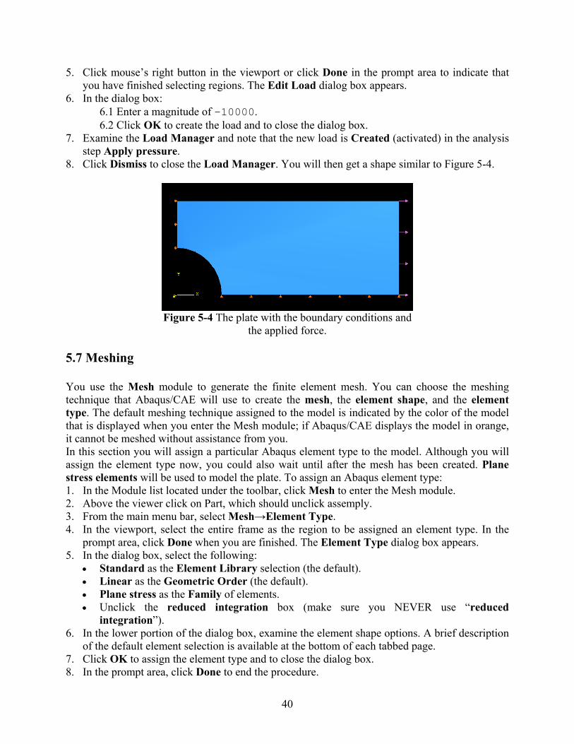
40

5. Click mouse’s right button in the viewport or click Done in the prompt area to indicate that you have finished selecting regions. The Edit Load dialog box appears.

6. In the dialog box: 6.1 Enter a magnitude of -10000. 6.2 Click OK to create the load and to close the dialog box.

7. Examine the Load Manager and note that the new load is Created (activated) in the analysis step Apply pressure.

8. Click Dismiss to close the Load Manager. You will then get a shape similar to Figure 5-4.

Figure 5-4 The plate with the boundary conditions and

the applied force.

5.7 Meshing You use the Mesh module to generate the finite element mesh. You can choose the meshing technique that Abaqus/CAE will use to create the mesh, the element shape, and the element type. The default meshing technique assigned to the model is indicated by the color of the model that is displayed when you enter the Mesh module; if Abaqus/CAE displays the model in orange, it cannot be meshed without assistance from you. In this section you will assign a particular Abaqus element type to the model. Although you will assign the element type now, you could also wait until after the mesh has been created. Plane stress elements will be used to model the plate. To assign an Abaqus element type: 1. In the Module list located under the toolbar, click Mesh to enter the Mesh module. 2. Above the viewer click on Part, which should unclick assemply. 3. From the main menu bar, select Mesh→Element Type. 4. In the viewport, select the entire frame as the region to be assigned an element type. In the

prompt area, click Done when you are finished. The Element Type dialog box appears. 5. In the dialog box, select the following:

Standard as the Element Library selection (the default). Linear as the Geometric Order (the default). Plane stress as the Family of elements. Unclick the reduced integration box (make sure you NEVER use “reduced

integration”). 6. In the lower portion of the dialog box, examine the element shape options. A brief description

of the default element selection is available at the bottom of each tabbed page. 7. Click OK to assign the element type and to close the dialog box. 8. In the prompt area, click Done to end the procedure.

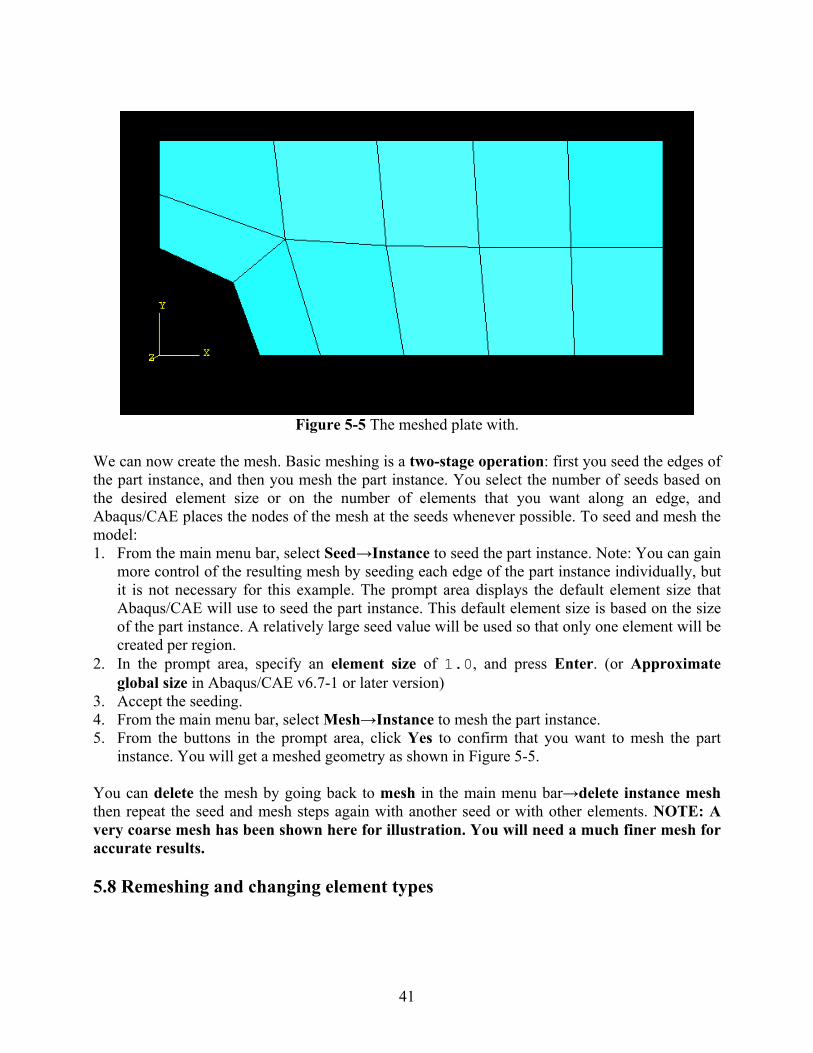
41

Figure 5-5 The meshed plate with.

We can now create the mesh. Basic meshing is a two-stage operation: first you seed the edges of the part instance, and then you mesh the part instance. You select the number of seeds based on the desired element size or on the number of elements that you want along an edge, and Abaqus/CAE places the nodes of the mesh at the seeds whenever possible. To seed and mesh the model: 1. From the main menu bar, select Seed→Instance to seed the part instance. Note: You can gain

more control of the resulting mesh by seeding each edge of the part instance individually, but it is not necessary for this example. The prompt area displays the default element size that Abaqus/CAE will use to seed the part instance. This default element size is based on the size of the part instance. A relatively large seed value will be used so that only one element will be created per region.

2. In the prompt area, specify an element size of 1.0, and press Enter. (or Approximate global size in Abaqus/CAE v6.7-1 or later version)

3. Accept the seeding. 4. From the main menu bar, select Mesh→Instance to mesh the part instance. 5. From the buttons in the prompt area, click Yes to confirm that you want to mesh the part

instance. You will get a meshed geometry as shown in Figure 5-5.

You can delete the mesh by going back to mesh in the main menu bar→delete instance mesh then repeat the seed and mesh steps again with another seed or with other elements. NOTE: A very coarse mesh has been shown here for illustration. You will need a much finer mesh for accurate results. 5.8 Remeshing and changing element types

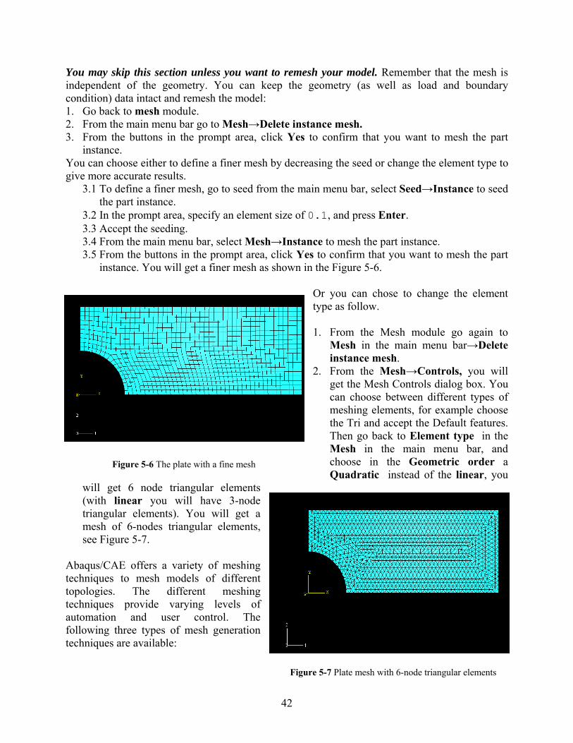
42

You may skip this section unless you want to remesh your model. Remember that the mesh is independent of the geometry. You can keep the geometry (as well as load and boundary condition) data intact and remesh the model: 1. Go back to mesh module. 2. From the main menu bar go to Mesh→Delete instance mesh. 3. From the buttons in the prompt area, click Yes to confirm that you want to mesh the part

instance. You can choose either to define a finer mesh by decreasing the seed or change the element type to give more accurate results.

3.1 To define a finer mesh, go to seed from the main menu bar, select Seed→Instance to seed the part instance.

3.2 In the prompt area, specify an element size of 0.1, and press Enter. 3.3 Accept the seeding. 3.4 From the main menu bar, select Mesh→Instance to mesh the part instance. 3.5 From the buttons in the prompt area, click Yes to confirm that you want to mesh the part

instance. You will get a finer mesh as shown in the Figure 5-6.

Or you can chose to change the element type as follow. 1. From the Mesh module go again to

Mesh in the main menu bar→Delete instance mesh.

2. From the Mesh→Controls, you will get the Mesh Controls dialog box. You can choose between different types of meshing elements, for example choose the Tri and accept the Default features. Then go back to Element type in the Mesh in the main menu bar, and choose in the Geometric order a Quadratic instead of the linear, you

will get 6 node triangular elements (with linear you will have 3-node triangular elements). You will get a mesh of 6-nodes triangular elements, see Figure 5-7.

Abaqus/CAE offers a variety of meshing techniques to mesh models of different topologies. The different meshing techniques provide varying levels of automation and user control. The following three types of mesh generation techniques are available:

Figure 5-6 The plate with a fine mesh

Figure 5-7 Plate mesh with 6-node triangular elements

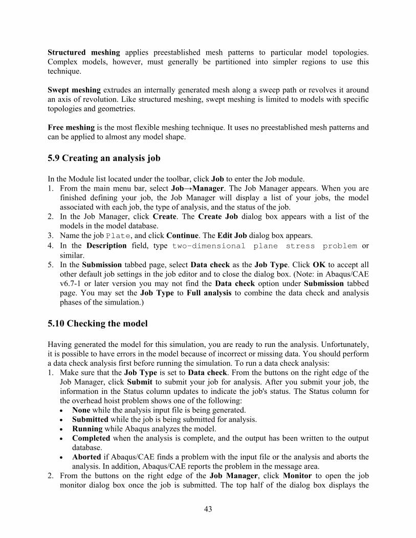
43

Structured meshing applies preestablished mesh patterns to particular model topologies. Complex models, however, must generally be partitioned into simpler regions to use this technique. Swept meshing extrudes an internally generated mesh along a sweep path or revolves it around an axis of revolution. Like structured meshing, swept meshing is limited to models with specific topologies and geometries. Free meshing is the most flexible meshing technique. It uses no preestablished mesh patterns and can be applied to almost any model shape. 5.9 Creating an analysis job In the Module list located under the toolbar, click Job to enter the Job module. 1. From the main menu bar, select Job→Manager. The Job Manager appears. When you are

finished defining your job, the Job Manager will display a list of your jobs, the model associated with each job, the type of analysis, and the status of the job.

2. In the Job Manager, click Create. The Create Job dialog box appears with a list of the models in the model database.

3. Name the job Plate, and click Continue. The Edit Job dialog box appears. 4. In the Description field, type two-dimensional plane stress problem or

similar. 5. In the Submission tabbed page, select Data check as the Job Type. Click OK to accept all

other default job settings in the job editor and to close the dialog box. (Note: in Abaqus/CAE v6.7-1 or later version you may not find the Data check option under Submission tabbed page. You may set the Job Type to Full analysis to combine the data check and analysis phases of the simulation.)

5.10 Checking the model Having generated the model for this simulation, you are ready to run the analysis. Unfortunately, it is possible to have errors in the model because of incorrect or missing data. You should perform a data check analysis first before running the simulation. To run a data check analysis: 1. Make sure that the Job Type is set to Data check. From the buttons on the right edge of the

Job Manager, click Submit to submit your job for analysis. After you submit your job, the information in the Status column updates to indicate the job's status. The Status column for the overhead hoist problem shows one of the following: None while the analysis input file is being generated. Submitted while the job is being submitted for analysis. Running while Abaqus analyzes the model. Completed when the analysis is complete, and the output has been written to the output

database. Aborted if Abaqus/CAE finds a problem with the input file or the analysis and aborts the

analysis. In addition, Abaqus/CAE reports the problem in the message area. 2. From the buttons on the right edge of the Job Manager, click Monitor to open the job

monitor dialog box once the job is submitted. The top half of the dialog box displays the

44

information available in the status (*.sta) file that Abaqus creates for the analysis. This file contains a brief summary of the progress of an analysis and is described in “Output,” Section 4.1.1 of the Abaqus Analysis User's Manual. The bottom half of the dialog box displays the following information: Log tab to display the start and end times for the analysis that appear in the log (*.log)

file. Errors and Warnings tabs to display the first ten errors or the first ten warnings that

appear in the data (*.dat) and message (*.msg) files. If a particular region of the model is causing the error or warning, a node or element set will be created automatically that contains that region. The name of the node or element set appears with the error or warning message, and you can view the set using display groups in the Visualization module. It will not be possible to perform the analysis until the causes of any error messages are corrected. In addition, you should always investigate the reason for any warning messages to determine whether corrective action is needed or whether such messages can be ignored safely. If more than ten errors or warnings are encountered, information regarding the additional errors and warnings can be obtained from the printed output files themselves.

Output tab to display a record of each output data entry as it is written to the output database.

5.11 Running the analysis Make any necessary corrections to your model. When the data check analysis completes with no error messages, run the analysis itself. To do this, edit the job definition and set the Job Type to Continue analysis; then, click Submit in the Job Manager to submit your job for analysis. You should always perform a data check analysis before running a simulation to ensure that the model has been defined correctly and to check that there is enough disk space and memory available to complete the analysis. However, it is possible to combine the data check and analysis phases of the simulation by setting the Job Type to Full analysis. If a simulation is expected to take a substantial amount of time, it may be convenient to run it in a batch queue by selecting Queue as the Run Mode. 5.12 Postprocessing with Abaqus/CAE When the job completes successfully, you are ready to view the results of the analysis with the Visualization module. From the buttons on the right edge of the Job Manager, click Results. Abaqus/CAE loads the Visualization module, opens the output database created by the job, and displays a fast plot of the model. A fast plot is a basic representation of the undeformed model shape and is an indication that you have opened the desired file. Alternatively, you can click Visualization in the Module list located under the toolbar, select File→Open, select Plate.odb from the list of available output database files, and click OK.

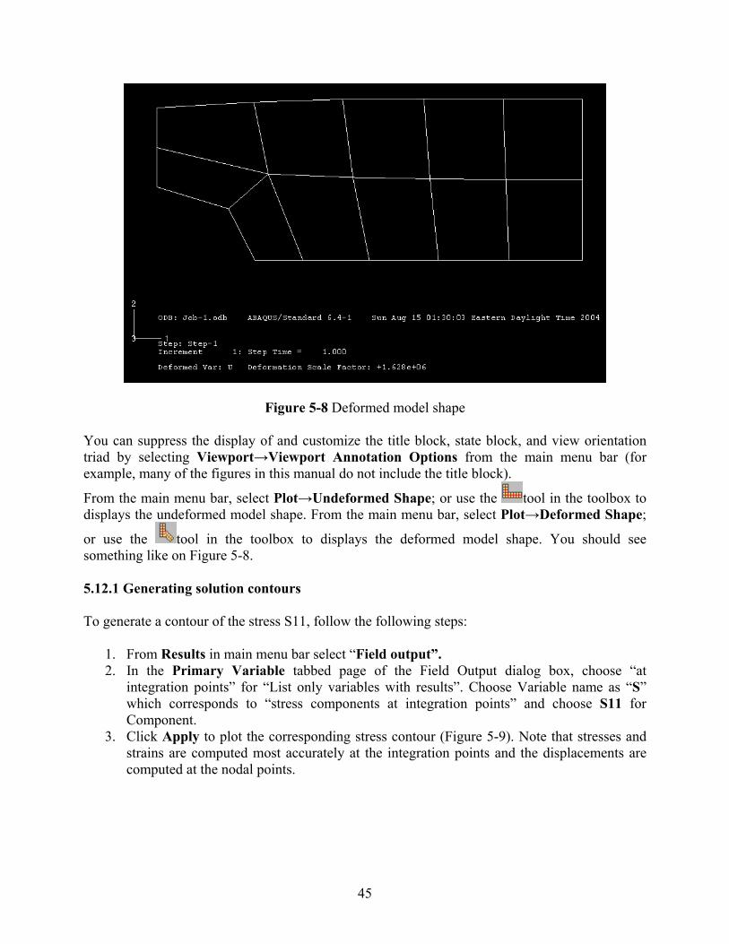
45

Figure 5-8 Deformed model shape

You can suppress the display of and customize the title block, state block, and view orientation triad by selecting Viewport→Viewport Annotation Options from the main menu bar (for example, many of the figures in this manual do not include the title block).

From the main menu bar, select Plot→Undeformed Shape; or use the tool in the toolbox to displays the undeformed model shape. From the main menu bar, select Plot→Deformed Shape;

or use the tool in the toolbox to displays the deformed model shape. You should see something like on Figure 5-8. 5.12.1 Generating solution contours To generate a contour of the stress S11, follow the following steps:

1. From Results in main menu bar select “Field output”. 2. In the Primary Variable tabbed page of the Field Output dialog box, choose “at

integration points” for “List only variables with results”. Choose Variable name as “S” which corresponds to “stress components at integration points” and choose S11 for Component.

3. Click Apply to plot the corresponding stress contour (Figure 5-9). Note that stresses and strains are computed most accurately at the integration points and the displacements are computed at the nodal points.

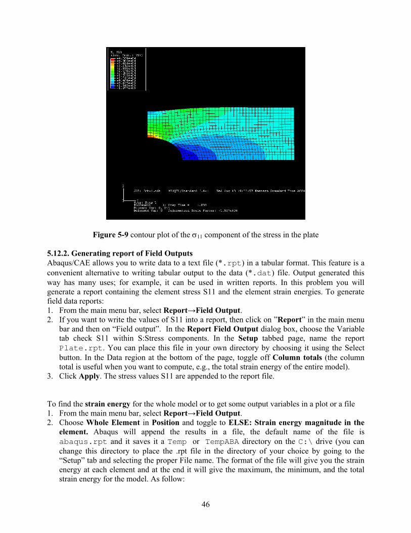
46

Figure 5-9 contour plot of the 11 component of the stress in the plate 5.12.2. Generating report of Field Outputs Abaqus/CAE allows you to write data to a text file (*.rpt) in a tabular format. This feature is a convenient alternative to writing tabular output to the data (*.dat) file. Output generated this way has many uses; for example, it can be used in written reports. In this problem you will generate a report containing the element stress S11 and the element strain energies. To generate field data reports: 1. From the main menu bar, select Report→Field Output. 2. If you want to write the values of S11 into a report, then click on ”Report” in the main menu

bar and then on “Field output”. In the Report Field Output dialog box, choose the Variable tab check S11 within S:Stress components. In the Setup tabbed page, name the report Plate.rpt. You can place this file in your own directory by choosing it using the Select button. In the Data region at the bottom of the page, toggle off Column totals (the column total is useful when you want to compute, e.g., the total strain energy of the entire model).

3. Click Apply. The stress values S11 are appended to the report file. To find the strain energy for the whole model or to get some output variables in a plot or a file 1. From the main menu bar, select Report→Field Output. 2. Choose Whole Element in Position and toggle to ELSE: Strain energy magnitude in the

element. Abaqus will append the results in a file, the default name of the file is abaqus.rpt and it saves it a Temp or TempABA directory on the C:\ drive (you can change this directory to place the .rpt file in the directory of your choice by going to the “Setup” tab and selecting the proper File name. The format of the file will give you the strain energy at each element and at the end it will give the maximum, the minimum, and the total strain energy for the model. As follow:

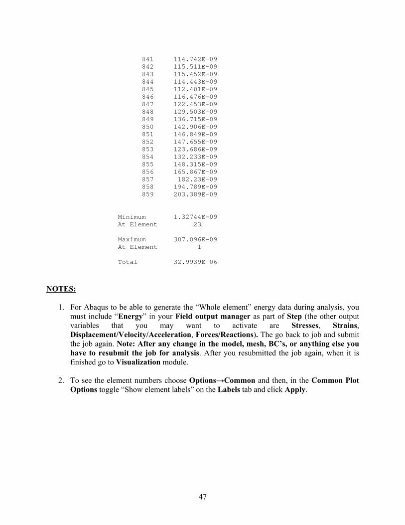
47

841 114.742E-09 842 115.511E-09 843 115.452E-09 844 114.443E-09 845 112.401E-09 846 116.476E-09 847 122.453E-09 848 129.503E-09 849 136.715E-09 850 142.906E-09 851 146.849E-09 852 147.655E-09 853 123.686E-09 854 132.233E-09 855 148.315E-09 856 165.867E-09 857 182.23E-09 858 194.789E-09 859 203.389E-09

Minimum 1.32744E-09 At Element 23 Maximum 307.096E-09 At Element 1 Total 32.9939E-06

NOTES:

1. For Abaqus to be able to generate the “Whole element” energy data during analysis, you must include “Energy” in your Field output manager as part of Step (the other output variables that you may want to activate are Stresses, Strains, Displacement/Velocity/Acceleration, Forces/Reactions). The go back to job and submit the job again. Note: After any change in the model, mesh, BC’s, or anything else you have to resubmit the job for analysis. After you resubmitted the job again, when it is finished go to Visualization module.

2. To see the element numbers choose Options→Common and then, in the Common Plot Options toggle “Show element labels” on the Labels tab and click Apply.

48

6. 3D EXAMPLE: Analysis of 3D elastic solid For complex 3D models, you may create your geometry directly using Abaqus or your favorite CAD software package and save it as one of the following formats that Abaqus reads and writes (make sure you read Abaqus/CAE User’s Manual regarding limitations): 3D XML (*.3dxml), ACIS (*.sat), AutoCAD (*.dxf) CATIA V4 (*.model, *.catdata, or *.exp), CATIA V5 Elysium Neutral File (*.enf_abq), I-DEAS Elysium Neutral File (*.enf_abq), IGES (*.igs), Output database (*.odb), Parasolid (*.x_t, *.x_b, *.xmt_txt, or *.xmt_bin), Pro/ENGINEER Elysium Neutral File (*.enf_abq), STEP (*.stp), VDA-FS (*.vda) and VRML (*.wrl). A file from a third-party CAD system, such as CATIA or Pro/ENGINEER, can contain a single part or an assembly of parts. Abaqus/CAE allows you to select File→Import from the main menu bar and choose either Part or Assembly. Both options allow you to import all of the parts in an assembly; however, the end result is slightly different. Importing parts If you choose to import parts from a file that contains an assembly of parts, you can import either all of the parts from the file or only a specified part. If you import all of the parts, Abaqus/CAE creates a group of parts that corresponds to each part instance in the original assembly. To recreate the original assembly, you must use the Assembly module to instance each imported part. However, the relationship between the parts and the part instances in the original assembly is lost during the import process. For example, if the original assembly contained a bolt that was instanced nine times, Abaqus/CAE creates nine identical parts. When you recreate the assembly in the Assembly module, Abaqus/CAE creates a part instance for each of the nine bolts. Although the relationship between the parts and part instances is lost, Abaqus/CAE does retain the position of the parts. As a result, when you instance each part, it appears in the correct position in the assembly. Importing an assembly If you choose to import an assembly, you can import the entire assembly or you can import only selected part instances. Abaqus/CAE appends your selection to the existing assembly and retains the original positioning of the instances. In addition, Abaqus/CAE creates parts that correspond to the imported part instances and maintains the relationship between the parts and their instances. For example, if a bolt is instanced nine times in the assembly, Abaqus/CAE imports nine instances of the bolt but creates only a single part. Importing an assembly also offers the following advantages:

In most cases Abaqus/CAE retains the names of the parts and the part instances from the

original file. If the parts and part instances in the original file were colored by the third-party CAD

system, Abaqus/CAE retains those colors during the import procedure.

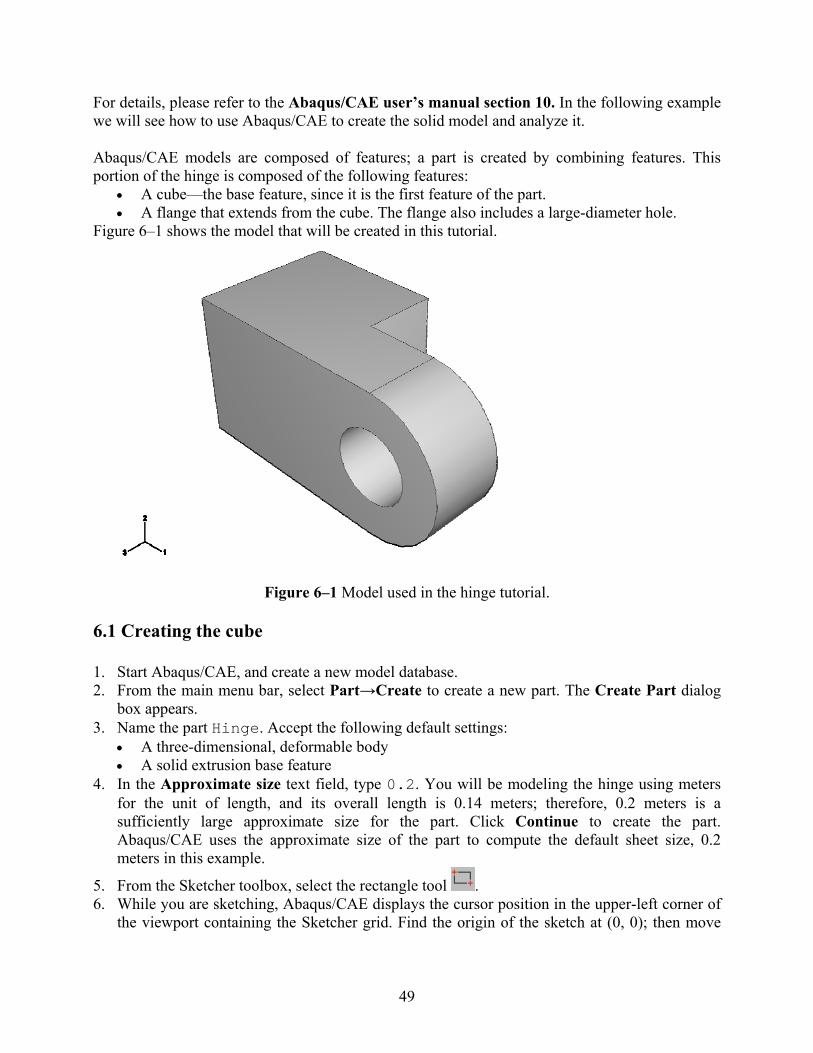
49

For details, please refer to the Abaqus/CAE user’s manual section 10. In the following example we will see how to use Abaqus/CAE to create the solid model and analyze it. Abaqus/CAE models are composed of features; a part is created by combining features. This portion of the hinge is composed of the following features:

A cube—the base feature, since it is the first feature of the part. A flange that extends from the cube. The flange also includes a large-diameter hole.

Figure 6–1 shows the model that will be created in this tutorial.

Figure 6–1 Model used in the hinge tutorial.

6.1 Creating the cube 1. Start Abaqus/CAE, and create a new model database. 2. From the main menu bar, select Part→Create to create a new part. The Create Part dialog

box appears. 3. Name the part Hinge. Accept the following default settings:

A three-dimensional, deformable body A solid extrusion base feature

4. In the Approximate size text field, type 0.2. You will be modeling the hinge using meters for the unit of length, and its overall length is 0.14 meters; therefore, 0.2 meters is a sufficiently large approximate size for the part. Click Continue to create the part. Abaqus/CAE uses the approximate size of the part to compute the default sheet size, 0.2 meters in this example.

5. From the Sketcher toolbox, select the rectangle tool . 6. While you are sketching, Abaqus/CAE displays the cursor position in the upper-left corner of

the viewport containing the Sketcher grid. Find the origin of the sketch at (0, 0); then move

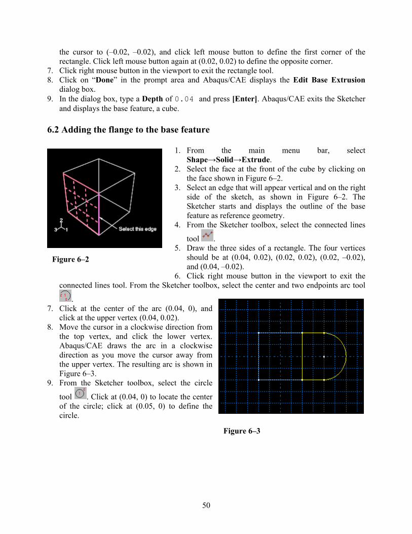
50

the cursor to (–0.02, –0.02), and click left mouse button to define the first corner of the rectangle. Click left mouse button again at (0.02, 0.02) to define the opposite corner.

7. Click right mouse button in the viewport to exit the rectangle tool. 8. Click on “Done” in the prompt area and Abaqus/CAE displays the Edit Base Extrusion

dialog box. 9. In the dialog box, type a Depth of 0.04 and press [Enter]. Abaqus/CAE exits the Sketcher

and displays the base feature, a cube. 6.2 Adding the flange to the base feature

1. From the main menu bar, select Shape→Solid→Extrude.

2. Select the face at the front of the cube by clicking on the face shown in Figure 6–2.

3. Select an edge that will appear vertical and on the right side of the sketch, as shown in Figure 6–2. The Sketcher starts and displays the outline of the base feature as reference geometry.

4. From the Sketcher toolbox, select the connected lines

tool . 5. Draw the three sides of a rectangle. The four vertices

should be at (0.04, 0.02), (0.02, 0.02), (0.02, –0.02), and (0.04, –0.02).

6. Click right mouse button in the viewport to exit the connected lines tool. From the Sketcher toolbox, select the center and two endpoints arc tool

. 7. Click at the center of the arc (0.04, 0), and

click at the upper vertex (0.04, 0.02). 8. Move the cursor in a clockwise direction from

the top vertex, and click the lower vertex. Abaqus/CAE draws the arc in a clockwise direction as you move the cursor away from the upper vertex. The resulting arc is shown in Figure 6–3.

9. From the Sketcher toolbox, select the circle

tool . Click at (0.04, 0) to locate the center of the circle; click at (0.05, 0) to define the circle.

Figure 6–2

Figure 6–3

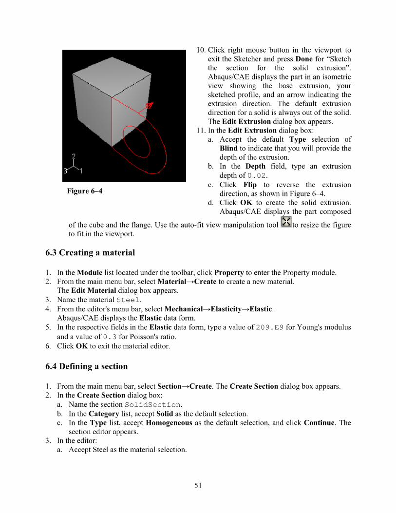
51

10. Click right mouse button in the viewport to exit the Sketcher and press Done for “Sketch the section for the solid extrusion”. Abaqus/CAE displays the part in an isometric view showing the base extrusion, your sketched profile, and an arrow indicating the extrusion direction. The default extrusion direction for a solid is always out of the solid. The Edit Extrusion dialog box appears.

11. In the Edit Extrusion dialog box: a. Accept the default Type selection of

Blind to indicate that you will provide the depth of the extrusion.

b. In the Depth field, type an extrusion depth of 0.02.

c. Click Flip to reverse the extrusion direction, as shown in Figure 6–4.

d. Click OK to create the solid extrusion. Abaqus/CAE displays the part composed

of the cube and the flange. Use the auto-fit view manipulation tool to resize the figure to fit in the viewport.

6.3 Creating a material 1. In the Module list located under the toolbar, click Property to enter the Property module. 2. From the main menu bar, select Material→Create to create a new material.

The Edit Material dialog box appears. 3. Name the material Steel. 4. From the editor's menu bar, select Mechanical→Elasticity→Elastic.

Abaqus/CAE displays the Elastic data form. 5. In the respective fields in the Elastic data form, type a value of 209.E9 for Young's modulus

and a value of 0.3 for Poisson's ratio. 6. Click OK to exit the material editor. 6.4 Defining a section 1. From the main menu bar, select Section→Create. The Create Section dialog box appears. 2. In the Create Section dialog box:

a. Name the section SolidSection. b. In the Category list, accept Solid as the default selection. c. In the Type list, accept Homogeneous as the default selection, and click Continue. The

section editor appears. 3. In the editor:

a. Accept Steel as the material selection.

Figure 6–4

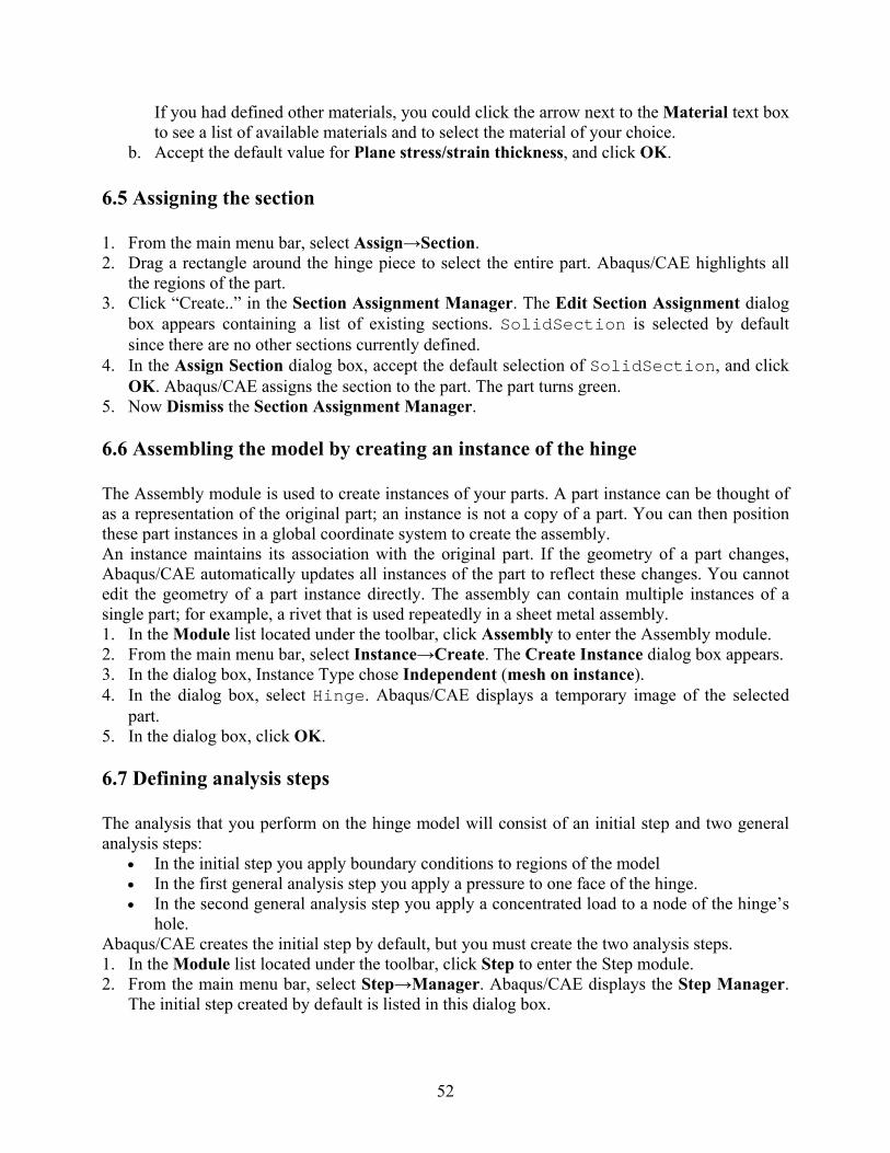
52

If you had defined other materials, you could click the arrow next to the Material text box to see a list of available materials and to select the material of your choice.

b. Accept the default value for Plane stress/strain thickness, and click OK. 6.5 Assigning the section 1. From the main menu bar, select Assign→Section. 2. Drag a rectangle around the hinge piece to select the entire part. Abaqus/CAE highlights all

the regions of the part. 3. Click “Create..” in the Section Assignment Manager. The Edit Section Assignment dialog

box appears containing a list of existing sections. SolidSection is selected by default since there are no other sections currently defined.

4. In the Assign Section dialog box, accept the default selection of SolidSection, and click OK. Abaqus/CAE assigns the section to the part. The part turns green.

5. Now Dismiss the Section Assignment Manager. 6.6 Assembling the model by creating an instance of the hinge The Assembly module is used to create instances of your parts. A part instance can be thought of as a representation of the original part; an instance is not a copy of a part. You can then position these part instances in a global coordinate system to create the assembly. An instance maintains its association with the original part. If the geometry of a part changes, Abaqus/CAE automatically updates all instances of the part to reflect these changes. You cannot edit the geometry of a part instance directly. The assembly can contain multiple instances of a single part; for example, a rivet that is used repeatedly in a sheet metal assembly. 1. In the Module list located under the toolbar, click Assembly to enter the Assembly module. 2. From the main menu bar, select Instance→Create. The Create Instance dialog box appears. 3. In the dialog box, Instance Type chose Independent (mesh on instance). 4. In the dialog box, select Hinge. Abaqus/CAE displays a temporary image of the selected

part. 5. In the dialog box, click OK.

6.7 Defining analysis steps The analysis that you perform on the hinge model will consist of an initial step and two general analysis steps:

In the initial step you apply boundary conditions to regions of the model In the first general analysis step you apply a pressure to one face of the hinge. In the second general analysis step you apply a concentrated load to a node of the hinge’s

hole. Abaqus/CAE creates the initial step by default, but you must create the two analysis steps. 1. In the Module list located under the toolbar, click Step to enter the Step module. 2. From the main menu bar, select Step→Manager. Abaqus/CAE displays the Step Manager.

The initial step created by default is listed in this dialog box.

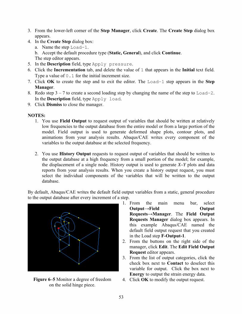
53

3. From the lower-left corner of the Step Manager, click Create. The Create Step dialog box appears.

4. In the Create Step dialog box: a. Name the step Load-1. b. Accept the default procedure type (Static, General), and click Continue. The step editor appears.

5. In the Description field, type Apply pressure. 6. Click the Incrementation tab, and delete the value of 1 that appears in the Initial text field.

Type a value of 0.1 for the initial increment size. 7. Click OK to create the step and to exit the editor. The Load-1 step appears in the Step

Manager. 8. Redo step 3 – 7 to create a second loading step by changing the name of the step to Load-2.

In the Description field, type Apply load. 9. Click Dismiss to close the manager. NOTES:

1. You use Field Output to request output of variables that should be written at relatively low frequencies to the output database from the entire model or from a large portion of the model. Field output is used to generate deformed shape plots, contour plots, and animations from your analysis results. Abaqus/CAE writes every component of the variables to the output database at the selected frequency.

2. You use History Output requests to request output of variables that should be written to the output database at a high frequency from a small portion of the model; for example, the displacement of a single node. History output is used to generate X–Y plots and data reports from your analysis results. When you create a history output request, you must select the individual components of the variables that will be written to the output database.

By default, Abaqus/CAE writes the default field output variables from a static, general procedure to the output database after every increment of a step.

1. From the main menu bar, select Output→Field Output Requests→Manager. The Field Output Requests Manager dialog box appears. In this example Abaqus/CAE named the default field output request that you created in the Load step F-Output-1.

2. From the buttons on the right side of the manager, click Edit. The Edit Field Output Request editor appears.

3. From the list of output categories, click the check box next to Contact to deselect this variable for output. Click the box next to Energy to output the strain energy data.

4. Click OK to modify the output request. Figure 6–5 Monitor a degree of freedom on the solid hinge piece.

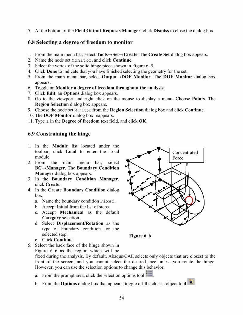
54

5. At the bottom of the Field Output Requests Manager, click Dismiss to close the dialog box. 6.8 Selecting a degree of freedom to monitor 1. From the main menu bar, select Tools→Set→Create. The Create Set dialog box appears. 2. Name the node set Monitor, and click Continue. 3. Select the vertex of the solid hinge piece shown in Figure 6–5. 4. Click Done to indicate that you have finished selecting the geometry for the set. 5. From the main menu bar, select Output→DOF Monitor. The DOF Monitor dialog box

appears. 6. Toggle on Monitor a degree of freedom throughout the analysis. 7. Click Edit, an Options dialog box appears. 8. Go to the viewport and right click on the mouse to display a menu. Choose Points. The

Region Selection dialog box appears. 9. Choose the node set Monitor from the Region Selection dialog box and click Continue. 10. The DOF Monitor dialog box reappears. 11. Type 1 in the Degree of freedom text field, and click OK. 6.9 Constraining the hinge 1. In the Module list located under the

toolbar, click Load to enter the Load module.

2. From the main menu bar, select BC→Manager. The Boundary Condition Manager dialog box appears.

3. In the Boundary Condition Manager, click Create.

4. In the Create Boundary Condition dialog box: a. Name the boundary condition Fixed. b. Accept Initial from the list of steps. c. Accept Mechanical as the default

Category selection. d. Select Displacement/Rotation as the

type of boundary condition for the selected step.

e. Click Continue. 5. Select the back face of the hinge shown in

Figure 6–6 as the region which will be fixed during the analysis. By default, Abaqus/CAE selects only objects that are closest to the front of the screen, and you cannot select the desired face unless you rotate the hinge. However, you can use the selection options to change this behavior.

a. From the prompt area, click the selection options tool .

b. From the Options dialog box that appears, toggle off the closest object tool .

Figure 6–6

Concentrated Force

55

c. Click over the desired face. Abaqus/CAE displays Next, Previous, and OK buttons in the prompt area.

d. Click Next and Previous until the desired face is highlighted. e. Click OK to confirm your choice.

6. Click right mouse button to indicate that you have finished selecting regions. The Edit Boundary Condition dialog box appears. The selection options return to the default setting of selecting only objects that are closest to the front of the screen.

7. In the dialog box: a. Toggle on the buttons labeled U1, U2, and U3 to constrain the end of the hinge in the 1-,

2-, and 3-directions. You do not need to constrain the rotational degrees of freedom of the hinge because solid elements (which have only translational degrees of freedom) will be used to mesh the hinge.

b. Click OK to close the dialog box. 8. Click Dismiss to close the dialog box. 6.10 Applying the pressure and the concentrated load to the hinge 1. From the main menu bar, select Load→Create. The Create Load dialog box appears. 2. In the Create Load dialog box:

a. Name the load Pressure. b. Accept Load-1 as the default selection in the Step text field. c. From the Category list, accept Mechanical as the default selection. d. From the Types for Selected Step list, select Pressure. e. Click Continue.

3. In the viewport, select the face at the end of the solid hinge piece as the surface to which the load will be applied (see face in Figure 6–6).

4. Click right mouse button to indicate that you have finished selecting regions. The Edit Load dialog box appears.

5. In the dialog box, enter a magnitude of –1.0E6 for the load, and click OK. Arrows appear on the face indicating the applied load. The arrows are pointing out of the face because you applied a negative pressure.

6. Redo steps 1-5 with naming the load Load, selecting Load-2 as the selection in Step text field. From the Types for Selected Step list, select Concentrated force. For the magnitude enter 1.0E4 for CF1.

6.11 Meshing the assembly Meshing the assembly is divided into the following operations:

Making sure the assembly can be meshed and creating additional partitions where necessary.

Assigning mesh attributes to the part instances. Seeding the part instances. Meshing the assembly.

When you enter the Mesh module, Abaqus/CAE color codes regions of the model according to the methods it will use to generate a mesh:

Green indicates that a region can be meshed using structured methods. Yellow indicates that a region can be meshed using sweep methods.

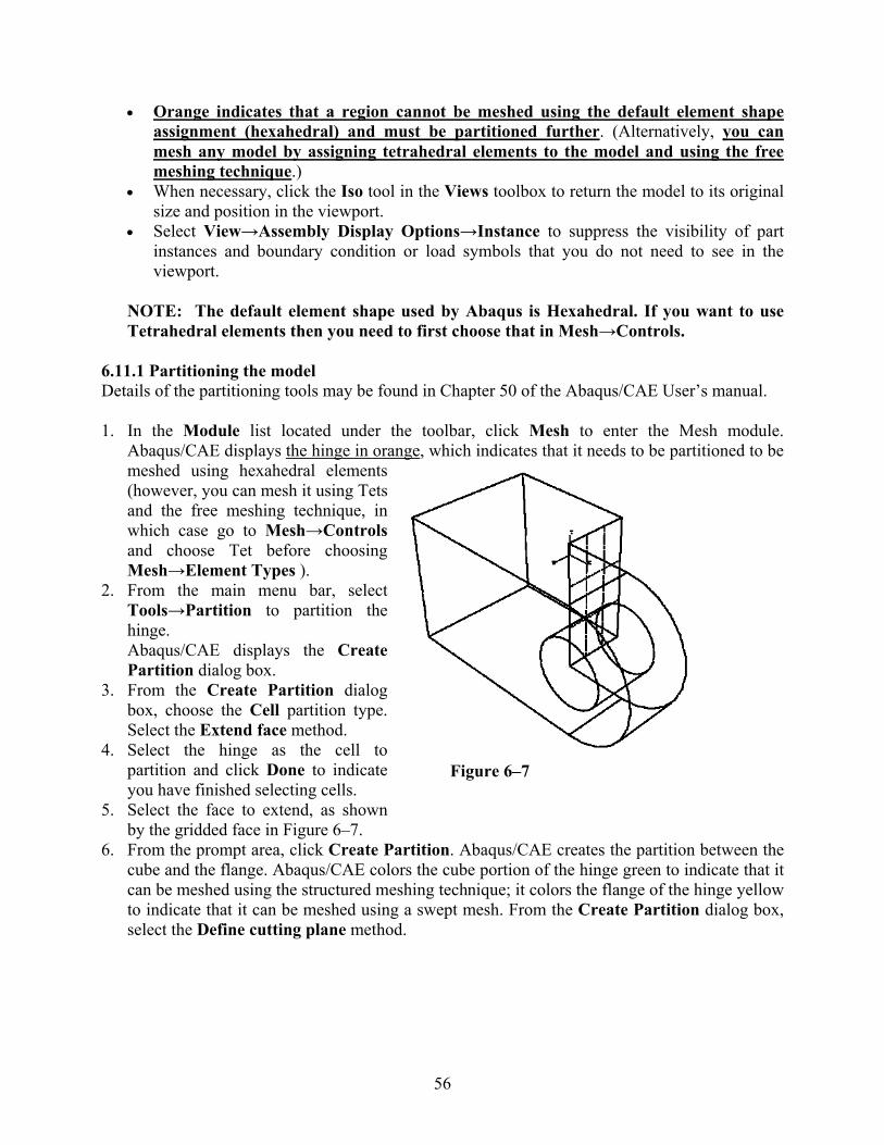
56

Orange indicates that a region cannot be meshed using the default element shape assignment (hexahedral) and must be partitioned further. (Alternatively, you can mesh any model by assigning tetrahedral elements to the model and using the free meshing technique.)

When necessary, click the Iso tool in the Views toolbox to return the model to its original size and position in the viewport.

Select View→Assembly Display Options→Instance to suppress the visibility of part instances and boundary condition or load symbols that you do not need to see in the viewport.

NOTE: The default element shape used by Abaqus is Hexahedral. If you want to use Tetrahedral elements then you need to first choose that in Mesh→Controls.

6.11.1 Partitioning the model Details of the partitioning tools may be found in Chapter 50 of the Abaqus/CAE User’s manual. 1. In the Module list located under the toolbar, click Mesh to enter the Mesh module.

Abaqus/CAE displays the hinge in orange, which indicates that it needs to be partitioned to be meshed using hexahedral elements (however, you can mesh it using Tets and the free meshing technique, in which case go to Mesh→Controls and choose Tet before choosing Mesh→Element Types ).

2. From the main menu bar, select Tools→Partition to partition the hinge. Abaqus/CAE displays the Create Partition dialog box.

3. From the Create Partition dialog box, choose the Cell partition type. Select the Extend face method.

4. Select the hinge as the cell to partition and click Done to indicate you have finished selecting cells.

5. Select the face to extend, as shown by the gridded face in Figure 6–7.

6. From the prompt area, click Create Partition. Abaqus/CAE creates the partition between the cube and the flange. Abaqus/CAE colors the cube portion of the hinge green to indicate that it can be meshed using the structured meshing technique; it colors the flange of the hinge yellow to indicate that it can be meshed using a swept mesh. From the Create Partition dialog box, select the Define cutting plane method.

Figure 6–7

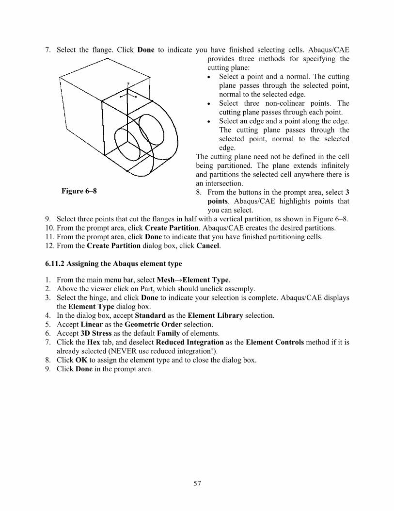
57

7. Select the flange. Click Done to indicate you have finished selecting cells. Abaqus/CAE provides three methods for specifying the cutting plane: Select a point and a normal. The cutting

plane passes through the selected point, normal to the selected edge.

Select three non-colinear points. The cutting plane passes through each point.

Select an edge and a point along the edge. The cutting plane passes through the selected point, normal to the selected edge.

The cutting plane need not be defined in the cell being partitioned. The plane extends infinitely and partitions the selected cell anywhere there is an intersection. 8. From the buttons in the prompt area, select 3

points. Abaqus/CAE highlights points that you can select.

9. Select three points that cut the flanges in half with a vertical partition, as shown in Figure 6–8. 10. From the prompt area, click Create Partition. Abaqus/CAE creates the desired partitions. 11. From the prompt area, click Done to indicate that you have finished partitioning cells. 12. From the Create Partition dialog box, click Cancel. 6.11.2 Assigning the Abaqus element type 1. From the main menu bar, select Mesh→Element Type. 2. Above the viewer click on Part, which should unclick assemply. 3. Select the hinge, and click Done to indicate your selection is complete. Abaqus/CAE displays

the Element Type dialog box. 4. In the dialog box, accept Standard as the Element Library selection. 5. Accept Linear as the Geometric Order selection. 6. Accept 3D Stress as the default Family of elements. 7. Click the Hex tab, and deselect Reduced Integration as the Element Controls method if it is

already selected (NEVER use reduced integration!). 8. Click OK to assign the element type and to close the dialog box. 9. Click Done in the prompt area.

Figure 6–8

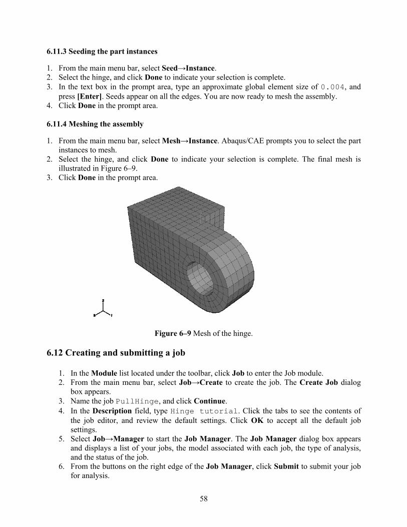
58

6.11.3 Seeding the part instances 1. From the main menu bar, select Seed→Instance. 2. Select the hinge, and click Done to indicate your selection is complete. 3. In the text box in the prompt area, type an approximate global element size of 0.004, and

press [Enter]. Seeds appear on all the edges. You are now ready to mesh the assembly. 4. Click Done in the prompt area. 6.11.4 Meshing the assembly 1. From the main menu bar, select Mesh→Instance. Abaqus/CAE prompts you to select the part

instances to mesh. 2. Select the hinge, and click Done to indicate your selection is complete. The final mesh is

illustrated in Figure 6–9. 3. Click Done in the prompt area.

Figure 6–9 Mesh of the hinge.

6.12 Creating and submitting a job

1. In the Module list located under the toolbar, click Job to enter the Job module. 2. From the main menu bar, select Job→Create to create the job. The Create Job dialog

box appears. 3. Name the job PullHinge, and click Continue. 4. In the Description field, type Hinge tutorial. Click the tabs to see the contents of

the job editor, and review the default settings. Click OK to accept all the default job settings.

5. Select Job→Manager to start the Job Manager. The Job Manager dialog box appears and displays a list of your jobs, the model associated with each job, the type of analysis, and the status of the job.

6. From the buttons on the right edge of the Job Manager, click Submit to submit your job for analysis.

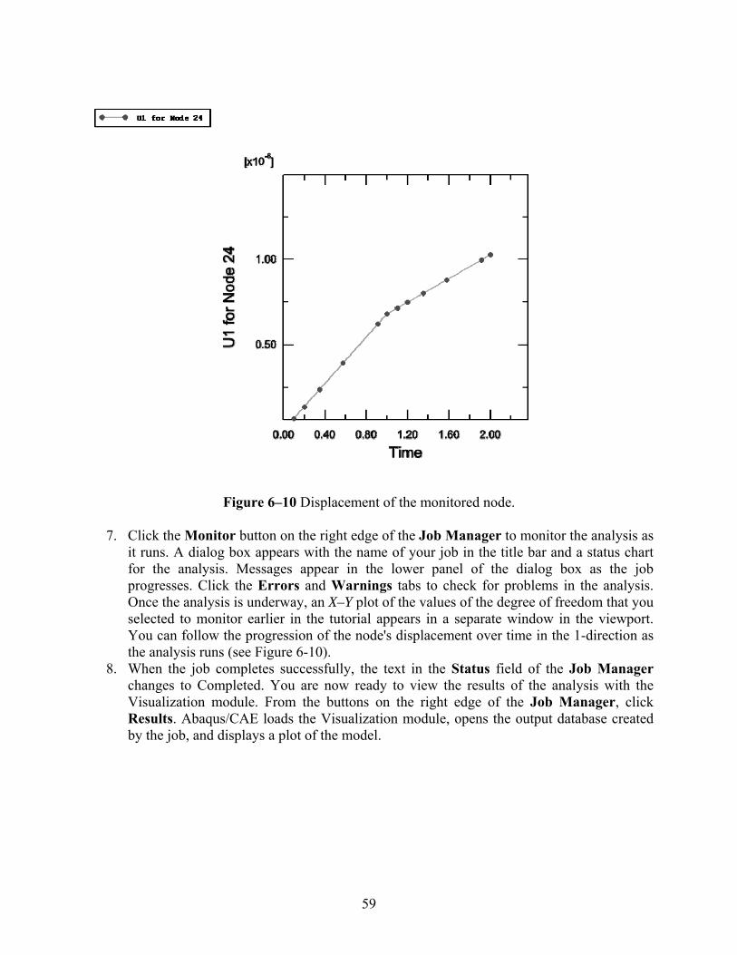
59

Figure 6–10 Displacement of the monitored node.

7. Click the Monitor button on the right edge of the Job Manager to monitor the analysis as

it runs. A dialog box appears with the name of your job in the title bar and a status chart for the analysis. Messages appear in the lower panel of the dialog box as the job progresses. Click the Errors and Warnings tabs to check for problems in the analysis. Once the analysis is underway, an X–Y plot of the values of the degree of freedom that you selected to monitor earlier in the tutorial appears in a separate window in the viewport. You can follow the progression of the node's displacement over time in the 1-direction as the analysis runs (see Figure 6-10).

8. When the job completes successfully, the text in the Status field of the Job Manager changes to Completed. You are now ready to view the results of the analysis with the Visualization module. From the buttons on the right edge of the Job Manager, click Results. Abaqus/CAE loads the Visualization module, opens the output database created by the job, and displays a plot of the model.

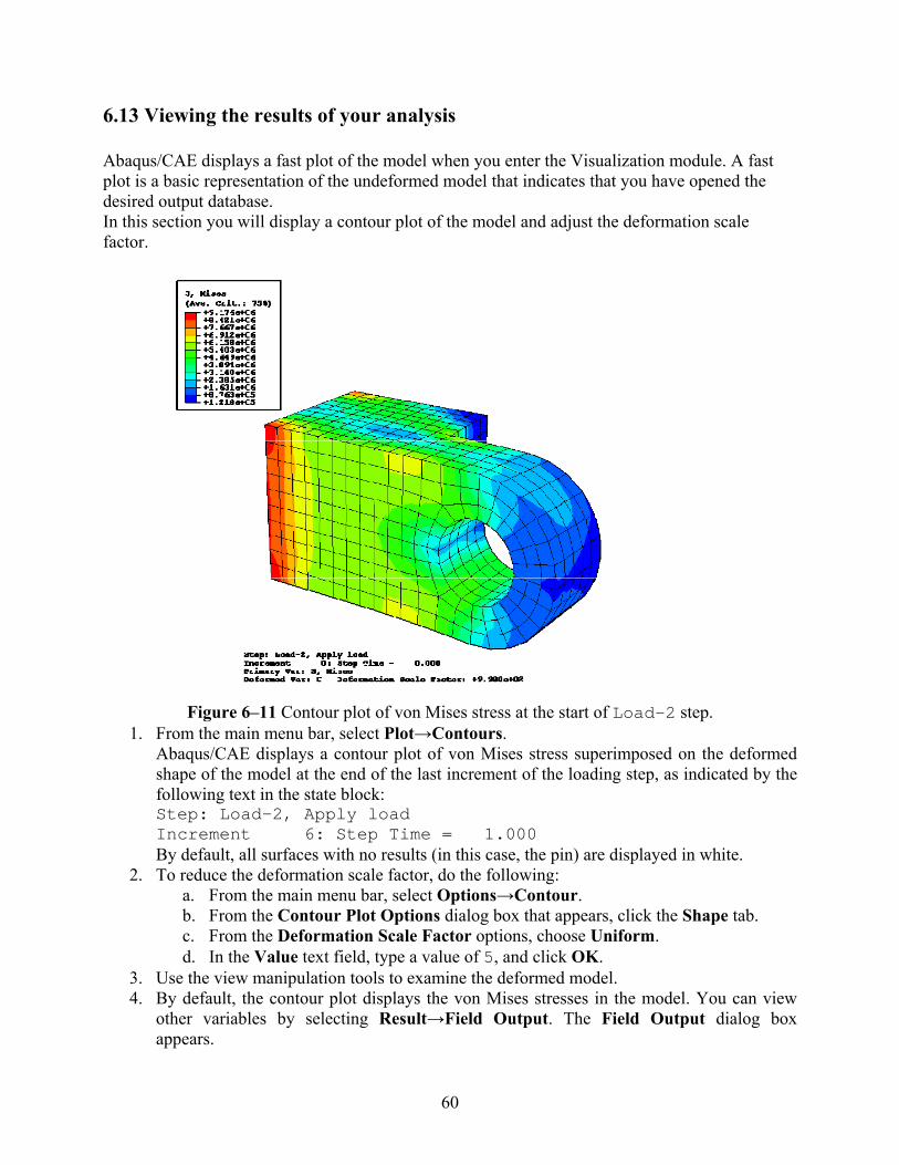
60

6.13 Viewing the results of your analysis Abaqus/CAE displays a fast plot of the model when you enter the Visualization module. A fast plot is a basic representation of the undeformed model that indicates that you have opened the desired output database. In this section you will display a contour plot of the model and adjust the deformation scale factor.

Figure 6–11 Contour plot of von Mises stress at the start of Load-2 step.

1. From the main menu bar, select Plot→Contours. Abaqus/CAE displays a contour plot of von Mises stress superimposed on the deformed shape of the model at the end of the last increment of the loading step, as indicated by the following text in the state block: Step: Load-2, Apply load Increment 6: Step Time = 1.000 By default, all surfaces with no results (in this case, the pin) are displayed in white.

2. To reduce the deformation scale factor, do the following: a. From the main menu bar, select Options→Contour. b. From the Contour Plot Options dialog box that appears, click the Shape tab. c. From the Deformation Scale Factor options, choose Uniform. d. In the Value text field, type a value of 5, and click OK.

3. Use the view manipulation tools to examine the deformed model. 4. By default, the contour plot displays the von Mises stresses in the model. You can view

other variables by selecting Result→Field Output. The Field Output dialog box appears.

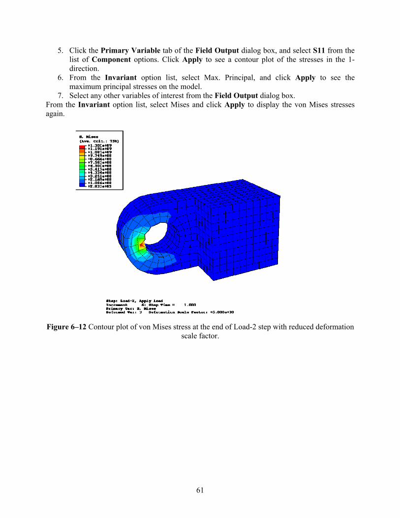
61

5. Click the Primary Variable tab of the Field Output dialog box, and select S11 from the list of Component options. Click Apply to see a contour plot of the stresses in the 1-direction.

6. From the Invariant option list, select Max. Principal, and click Apply to see the maximum principal stresses on the model.

7. Select any other variables of interest from the Field Output dialog box. From the Invariant option list, select Mises and click Apply to display the von Mises stresses again.

Figure 6–12 Contour plot of von Mises stress at the end of Load-2 step with reduced deformation

scale factor.