March 2003 Draft: Not for citation

Abilities, Budgets and Age: Inter-Generational Economic Mobility in Finland

Robert E.B. Lucas Boston University

Sari A. Pekkala

VATT (Government Institute for Economic Research, Finland) The authors are most grateful to the Academy of Finland for partial funding of this study under project number 52198.

Two distinct explanations have been postulated for the observed positive correlation between incomes of children and those of their parents. Where credit constraints are prevalent, parental wealth may restrict investment in human capital of children. Alternatively, unobserved abilities that are positively associated with earnings may be passed between generations, either genetically or through the home environment, resulting in an auto-regressive process in earnings across generations. Empirical distinction between these two hypotheses has proved elusive. A model combining both features is outlined and estimated here. The data are drawn from a very remarkable and largely unexplored panel encompassing the entire Finnish

2

population from 1970 to 1999. The results suggest that the budget constraint is much the larger of the two effects; only weak support is found consistent with the hypothesis of inherited earning ability. In the process of developing these results, a number of additional issues are addressed. Most of the existing evidence on inter-generational transmission of economic inequality refers to sons and fathers in the US, imposing a lower bound on the age of sons sampled, and omitting observations with zero or low earnings. The Finnish data permit inclusion of both daughters and mothers. A simple, theoretical extension is also explored which results in the elasticity of inter-generational transmission varying systematically with age of the child. In the Finnish context, our estimates indicate that the inter-generational transmission elasticity rises with age of both sons and daughters, though more strongly so for sons. This finding suggests a potential explanation as to why US estimates have proved sensitive to the age cut-off of sons in the sample. US estimates of the inter-generational correlation of earnings between fathers and sons have also been shown to be upward biased by sample selection rules that omit zero and low earnings observations. In the Finnish context, the opposite is demonstrated and some evidence on underlying reasons is presented. Section I outlines the simple theoretical framework, the transition to a measurement model, and some issues that arise in estimation. The Finnish data are described in greater detail in Section II, together with a brief review of prior analyses of inter-generational transmission of inequality in Finland based on portions of these data. Section III discusses specification and presents the mains results. Prior results on the Scandinavian countries indicate a fairly high degree of inter-generational mobility.1 The results in Section III indicate that this is less true for Finland than previously thought and Section IV closes by attempting to put these fresh results in perspective.

I. Theory and Estimation Three aspects of the theory of inter-generational transmission of inequality are taken up in this section. In part (a), a model of inter-generational transmission is sketched, emphasizing the difference between contexts with and without credit constraints. Part (b) then addresses formulation of counterpart measurement models, when available data offer only snapshots of incomes or earnings over a limited time span, representing their permanent counterparts with error. In this representation, the standard approach is

1 See, for example, Björklund and Jäntti (1997) and Björklund et al. (2000). On comparisons between Scandinavia and the US of income mobility within a generation, see Aaberge et al. (1996).

3

extended to incorporate an interaction between age and human capital in the determination of observed earnings, requiring a simple modification to the conventional treatment of permanent income and life-time earnings. Lastly, part (c) turns to consideration of some issues that arise in estimation.

a. A model of inter-generational transmission: with and without credit constraints. The wealth model of Becker and Tomes (1986) is in the class of consensus, parental preference models, in which children play no role in decision making. (Behrman, 1997). Mulligan (1999) lends specificity to this wealth model by assuming a single child family in which the utility (Up) of the parent takes a CES form:

1. Up = [Cp 0 + ∀ Yc 0 ] 1/0 where Cp represents consumption of the parent, Yc is permanent income (or wealth ) of the child, ∀ is the weight placed on altruism and (1-0)-1 is the elasticity of substitution. The parent chooses an amount (Hc) to invest in the child’s human capital, bequests and intervivos transfers (Bc) to be passed to the child, and their own consumption level to maximize (1), subject to two constraints. The first is a budget constraint:

2. Cp +Hc +Bc Yp where Yp represents wealth of the parent. Second, each child’s wealth is generated from the child’s human capital and transfers such that:

3. Yc = GcHc ∆ + Bc (1+4) where Gc denotes inherent capacities of the child to generate earnings, ∆ is the return on human capital (with 0<∆<1) and 4 is the rate of interest obtained on transfers.2 In the event that an interior solution exists for both Hc and Bc, the first order conditions may be solved to provide:

4. Hc = [∆Gc (1+4) -1 ]1/ (1-∆) This outcome is illustrated for the case of positive transfers in Figure 1. The parent’s wealth is marked P on the horizontal axis. As the parent invests some portion of their wealth in human capital of the child, the child’s life-time earnings rise along the curve PP’, conditioned upon inherent earning capacity Gc. The parent elects to invest in the child’s human capital such that the budget line from returns on transfers is tangent to PP’. An indifference curve, drawn for this wealth model, completes the choice of transfers and parental consumption at point W. Note that since the budget constraint is linear in this range, the parent’s choice of Hc is independent of the elasticity of substitution assumed in drawing the indifference curve, and hence 0 does not appear in (4). 2 Note that in this simple treatment, ∆, 4 and Gc are assumed known by the parent and that ∆ and 4 are common. Mulligan adds to (3) a multiplicative stochastic term, which can be thought of as luck of the child affecting both components of income symmetrically. For simplicity of exposition this term is suppressed here. See, however, Abul Naga (2002) for implications of this additional stochastic term with respect to estimation.

4

On the other hand, if the choice between parental consumption and child’s wealth lies at point W’ in Figure 1, then negative transfers (borrowing against the child’s wealth at the same rate 4) would be required to sustain such an interior solution. This may well be infeasible. If credit constraints restrict transfers to be non-negative, then the optimal choice of the parent in this case is at point C. The amount of investment in human capital at C is given from the first order condition on maximizing (1) with respect to Hc, subject to (2), (3) and the additional constraint that Bc 0. When this last constraint is binding, the solution has the implicit form:

5. Yp = Hc + [∆∀ Gc0 Hc ∆0-1] 1/(0-1)

in which Hc/ Yp>0, given Gc. In the instance of a Cobb-Douglas utility function 0 = 0 and (5) reduces to the more tractable, explicit form:

6. Hc = Yp ∆∀ (1+∆∀) -1 For convenience, the case depicted by W in Figure 1 is referred to as the wealth model in the remainder of this paper, while C is termed the credit constrained case. Note that a critical distinction appears between the solution to these cases. In the wealth model, investments in the child’s human capital are affected only by the child’s inherent earning capacity Gc and, in particular, parental wealth does not appear in (4). In contrast, in the credit constrained case, parental wealth indeed affects the child’s human capital directly in both (5) and (6). Thus, in the credit constrained case, parental wealth already impacts that of the child through the budget constraint, but in the wealth model another factor must be introduced to generate an autoregressive process in earnings across generations. In Becker and Tomes (1986), this additional factor is a presumption of autoregression in inherent earnings capacity, akin to the seminal ideas of Galton (1869), embodying an unknown mix of genetic and cultural transmissions,

7. Gc = GpΡ (c

where Gp is the inherent earning capacity of the parent, (c is a stochastic component in this inheritance and 0< Ρ < 1. Let Ec represent a component of the child’s wealth which we may call life time earnings, such that,

8. Ec GcHc ∆ In the case of the wealth model, one can then substitute in (8) for Hc from (4) to provide

9. Ec = [(1+4) ∆-1 ]∆/ (∆-1) Gc 1/ (1-∆)

If investments in the parent’s human capital were also dictated by the wealth model, then a relationship equivalent to (9) holds for the parent’s earnings too and may be inverted as

10. Gp = Ep 1-∆* [(1+4*) -1 ∆*]- ∆* where Gp, Ep, 4* and ∆* correspond in the parent’s generation to Gc, Ec, 4 and ∆ in the case of the child. From (10), (7) and (4), investment in the child’s human capital in the wealth model is then given by

11. Hc = {EpΡ (1-∆*) [∆(c (1+4) -1] [(1+4*)-1 ∆*] -Ρ∆*}1 / (1-∆)

5

Moreover, combining (7), (9) and (10) yields the inter-generational, autoregressive earnings structure in this wealth model

12. Ec = 60 Ep Ρ (1-∆*) / (1-∆) (c1 / (1-∆) in which 60 depends only upon the parameters 4, ∆, 4*, ∆* and Ρ. Note the implication that, if the returns on human capital remain approximately constant, (that is ∆ ∆*), then the elasticity of the child’s life time earnings with respect to earnings of the parent simply represents the elasticity of transmission of inherent earnings ability, Ρ, in this model. However, if ∆ > ∆*, then the elasticity of inter-generational transmission of earnings in (12) is greater than the transmission of inherent abilities. Figure 2 illustrates the outcome as parental wealth increases in the context of both models. PP represents the boundary of opportunities open to a family with a lower level of wealth. For a family with greater wealth, but either the parent’s ability is similar to that of the poorer parent or any additional ability is not transmitted to the child (Ρ=0), the boundary is defined by QQ. On the other hand, if the parent in the wealthier family has greater ability and transmits some of that ability to the child then their opportunity set is defined by QR. In the case of the wealth model, a pure income effect in going from PP to QQ does not change investments in the child’s human capital which remains at level h1. The child’s earnings are unaffected and so Yp does not appear in (12). The child’s wealth is increased, even in this case, but this is entirely through bequests rather than enhanced earnings. On the other hand, if the source of additional wealth of the parent reflects greater earnings that are correlated with ability of the parent, and if this ability is partially transmitted to the child, then the opportunity set of the parent with greater earnings is bounded br QR. For the parent with greater earnings, investment in the child’s human capital is h2, which is greater than h1, and positive auto-regression in inter-generational earnings results, as in (12). For any credit constrained family with homothetic preferences, investment in human capital expands with wealth even when Ρ=0, such that point 2 lies above point 1 in Figure 2. Whether human capital investments are amplified if Ρ>0 depends upon the shape of preferences for these credit constrained families. For instance, in the case of a Cobb-Douglas utility function, human capital investments are independent of Gc and hence independent of inherent ability transmission, as may be seen from (6). If QR and QQ represent children with different levels of ability, but from families with equal wealth, point 3 would lie vertically above point 2 in the Cobb-Douglas case. Nonetheless, the child’s earnings remain enhanced directly by inherent abilities in (8), so combining (8) with (6), (7) and (10) provides:

13. Ec = 61 Yp ∆ Ep Ρ (1-∆*) (c where 61 is a function of the parameters ∀, ∆, 4*, ∆* and Ρ. In (13), parental wealth enhances the child’s earnings through a budget constraint effect and the parent’s earnings are correlated with parental ability,

6

and hence the child’s ability and earnings, provided Ρ>0.3

b. Snapshots: observed incomes within generations. The theoretical approaches, outlined in part (a), manage to abstract from consideration of events arising within a generation by focusing on permanent incomes and life-time earnings. The empirical researcher does not have this luxury; permanent incomes are unobservable and data on life-time earnings are nowhere available to date. Estimation of equations such as (12) or (13) must rely, instead, upon observed incomes or earnings of individuals and of their parents, tracked over some limited duration within the life-cycle. Additional assumptions are then required linking these observed measures on earnings and incomes to their permanent counterparts modeled above. To illustrate the approach adopted for present purposes, consider the following expression:

14. ect = ,c0 + ,1 act + ,2 act nHc + >ct where ect and act are the natural logarithm of child c’s observed earnings and c’s age at time t, respectively;

nHc is the logarithm of c’s human capital, ,c0 is a fixed effect for person c, ,1 and ,2 are parameters and >ct is a stochastic disturbance term. More typically, additional polynomial terms in age are also incorporated into (14), but these are omitted here for brevity and without loss of generality, although we shall return to this issue in the empirical implementation. There is a remarkable uniformity in the existing, empirical literature on inter-generational mobility in presuming that ,2 = 0 in (14). In view of the substantial evidence of significant interaction effects between age (or experience) and schooling, in the estimation of earnings equations, such a presumption seems particularly onerous.4 Nonetheless, defining units such that Eact = 1 and assuming that E >ct = 0, where E

signifies a mean over a fixed number of lifetime periods, the presumption that ,2 = 0 implies lifetime

3 Note that the use of (10) in deriving (13) presupposes that human capital investments in the parent, made by grandparents, were not credit constrained. If, instead, the human capital of the parent were formed in a credit constrained process, then using parental equivalents to the human capital choice (6) and earnings definition (8) then inverting the latter yields:

Gp = Ep Yg -∆* [(1+∆*∀*) (∆*∀*) -1 ]∆* where Yg represents the wealth of the grandparents. Using this in conjunction with (6) and (8) then provides a second-order, autoregressive, inter-generational transmission process:

Ec = 62 Yp ∆ Ep Ρ Yg -Ρ∆* (c where 62 is a function of ∀, ∆, ∀*, ∆* and Ρ In practice, lacking three-generations of family data, almost all of the empirical attention has focused on estimation of a two-generation process. See, however, Behrman and Taubman (1985) and Warren and Hauser (1997).

4 Moreover, the adoption of earnings (as opposed to wage rate) measures in much of the existing evidence on inter-generational mobility would suggest an age-human capital interaction, particularly at younger ages, to the extent that students work shorter hours.

7

earnings simply amount to ,c0 + ,1. More generally, however, when the time profile of earnings varies across individuals, as in (14), relying upon the person-specific intercepts of these profiles to proxy permanent earnings will not suffice. Nonetheless, in this more general case, the logarithm of a child’s lifetime earnings may be defined in relation to the observed ect by:5

15. nEc = E ect

Then, using (15), ,c0 can be replaced in (14) to leave: 16. ect = nEc - ,1 - ,2 nHc +,1 act +,2 act nHc + >ct

Obviously, the conventional approach emerges as a special case within (16), in which ,2 =0. In the case without credit constraints, nHc may now be replaced in (16) by the logarithm of Hc from (11), while Ec is given in (12). This leaves:

17. ect = Τ0 + Τ1 nEp + Τ2 act nEp + Τ3 act + Λct A similar transformation for the credit constrained case, using (6) and (13) yields:

18. ect = Β0 + Β1 nEp + Β2 nYp + Β3 act nYp + Β4 act +Πct Certainly the inclusion of the age-human capital interaction term in (14) adds a potentially important element to the estimation of inter-generational effects. In particular, no matter whether the credit constraint is assumed to be binding or not, the implication is that the magnitude of inter-generational transmission rises with age of the child, provided that ,2>0. As a result, existing estimates indeed prove quite sensitive to the age range over which children are observed, as emphasized in Reville (1995). To proceed to consider estimation it remains to replace the permanent income and parental life-time earnings with a measured counterpart. In particular, let:

19.i. epϑ = ,p0* + ,1* apϑ + ,2* apϑ sp + >pϑ 19.ii. ypϑ = µp0* + µ1* apϑ + µ2* apϑ sp + .pϑ

where apϑ is age, while epϑ and ypϑ are the logarithms of some measure of earnings and income, respectively, for parent p (of child c) at time ϑ; sp represents the education level of p, ,p0* and µp0* denote personal fixed effects, ,1*, ,2*, µ1* and µ2* are parameters, and >pϑ and .pϑ are stochastic disturbance terms.6 Proceeding as in (15) and (16) for children, (19) provides: 5 A discount factor, common across individuals, can readily be inserted into (15) without appreciably affecting results.

6 The main reason for including sp in (19), rather than the logarithm of the parent’s human capital in keeping with (14), is pragmatic. One could proceed to substitute for the logarithm of parent’s human capital in terms of earnings and/or income of the grandparents, in parallel with (17) and (18) for the children. However, this would require a third generation of data on grandparents which is rarely available. A third generation of data does exist for Finland, but is not yet available at the time of writing. On the other hand, if sp is considered a proxy for parent’s human capital then a measurement error is introduced, though this error is not modeled explicitly here. Note that the conventional route is to presume that ,2*=0 (or that µ2* =0 if a measure of parental income is used instead), in which case the issue of representing parent’s schooling in (19) is moot. It might be noted that such a presumption is not

8

20.i. nEp = epϑ - ,1* apϑ - ,2* apϑ sp +,1* +,2* sp - >pϑ 20.ii. nYp = ypϑ - µ1* apϑ - µ2* apϑ sp +µ1* +µ2* sp - .pϑ

where E >pϑ and E .pϑ are again assumed to be zero. Lastly, (20) may be combined with either (17) or (18)

to provide a generic, population regression model: 21. ect = 20 + 21 epϑ + 22 ypϑ + 23 act epϑ + 24 act ypϑ + 25 act + 26 apϑ +

27 actapϑ + 28 sp + 29 sp apϑ + 210 act sp + 211 act sp apϑ + 1ct Noting in particular that:

Without credit constraint With credit constraint

21 = Τ1 = Ρ (1-∆*)(1-∆)-1 (1- ,2 ) 22 = 0 23 = Τ2 = Ρ (1-∆*)(1-∆)-1 ,2 24 = 0

21 = Β1 = Ρ (1-∆*) 22 = Β2 = ∆ - ,2 23 = 0 24 = Β3 = ,2

Equation (21) is certainly simplified considerably if the conventional assumption about parents is maintained such that µ2*= ,2*=0, in which case 28 = 29 = 210 = 211 =0. If, in addition, ,2 =0 for children in (14), then 23= 24 = 27 = 0. It is also important to note that the wealth model, without credit constraints, suggests that 22 = 24 = 0, even if ,2 0. Moreover, in the credit constrained model, 23 = 0 (even if ,2 0) and 21 = 0 if Ρ=0 in which case inherited traits are unimportant. Together theses suggest a number of hypotheses that, in principle, may be explored in relation to the data. Before turning to do so, however, it is worth pausing to consider the stochastic components underlying the disturbance term 1ct in (21).

c. Issues in estimation From (17), (18) and (20), the disturbance terms in the population regression models for the case with no binding credit constraint (Σct) and when a credit constraint is binding (Αct) are given by:

22.i. Σct = (1-∆)-1(1+,2 act- ,2) n(c - (21 + 23 act) >pt + >ct 22.ii. Αct = n(c - (22 + 24 act) .pt - 21 >pt + >ct

Both expressions include time dependent errors in measurement from representing the parent’s life-time earnings or permanent income by a short panel of observations (>pt or .pt). The well-known consequence is that ordinary least squares, applied to equations similar to (21), generates inconsistent estimates. Two main approaches have been adopted to address this inconsistency. The first approach has been called the method of averages, in which parental earnings or incomes are measured by a time-series mean over the period of observation on parents.7 Abul Naga (2002) considers necessarily inconsistent with retaining an age-human capital interaction in (14) since parents are normally observed at more mature ages, by which time such an interaction may have diminished. Once again, (19) is typically modeled as a higher order polynomial in age, and the empirical portion of this paper will do so too, but for brevity in notation the linear form will suffice for the moment.

7 Berhman and Taubman (1990), Altonji and Dunn (1991), Solon (1992).

9

some properties of such a method of averages estimator for a relatively simple, wealth model with no age interaction. In current notation this may be written:8

23. ect = 20 + 21 epϑ + (1-∆)-1 n(c - 21 >pt + >ct Assuming that the three stochastic components, n(c, >pt and >ct, are stationary, homoskedastic and mutually uncorrelated, Abul-Naga notes that the probability limit for the ordinary least squares estimator of 21 in (23) is:

^ 24. plim 21 = 21 - 21 Φ>p

2/Tp

(1-∆*)2ΦGp2 + Φ>p

2/Tp where ΦGp

2 is the variance of nGp, Φ>p2 is the variance of >pt and Tp represents the number of periods

over which the parent’s earnings are averaged.9 The estimator in (24) is biased toward zero, but the extent of asymptotic bias diminishes with Tp. In his survey Solon (1999) stresses the importance of larger values of Tp and some testing along these lines is reported in Section III of this paper. A second, though less common, approach to the errors-in-measurement in (22) has been to instrument a single year of data on a parent’s earnings. An appropriate instrument should be correlated with the parent’s permanent earnings but not with the transitory component of earnings. Solon (1992), Björklund and Jäntti (1997) Dearden, Machin and Reed (1997) and Abul Nagar (2002) have each considered the use of a parent’s education as an instrumental variable in this context. This choice of instrumental variable could bias results, if the parent’s education is an argument of the population regression but omitted from the measurement model. However, Solon (1992) argues that any such bias is likely to be small and Abul Nagar (2002), using a Sargan test on the same data set explored by Solon, fails to reject parental education as a valid instrument. On the other hand, parent’s education does appear in the generic regression model (21), a reflection of a possible interaction between age and schooling in affecting transitory income of the parent.10 Either a model with 28 through 211 =0 is appropriate and parental education may represent a valid instrument, or alternative instruments must be sought.11

8 Abul Naga (2002) retains the multiplicative, stochastic luck term in income realization (3) introduced by Mulligan (1999) but, as noted previously, suppressed here for brevity. These terms, for both the child and parent, consequently also appear additively in Abul Naga’s specification of (23) with the latter multiplied by 21.

9 Note that the denominator of the second term on the right follows from the variance of the parent’s life-time earnings in the inverse of (10).

10 Education of parents may also affect the child’s earnings through at least two other routes not modeled here: by affecting the child’s abilities, augmenting the arguments in (7), or by affecting the tastes of parents.

11 See Zimmerman (1992), Mulligan (1997,1999) and Abul Nagar (2002) for explorations with alternative instruments.

10

In instances where multiple time-period observations on the earnings of the child are available, a number of estimation options have been explored. In his initial approach, Zimmerman (1992) treats each year of data on sons’ earnings in cross section, noting the mean of these independent estimates. Abul Nagar (2002) notes that a more efficient estimator of this mean across time periods is obtained from a between-individual estimator, adopting the mean earnings of the child as dependent variable, provided that the transitory components of the child’s and parent’s earnings are stationary. Such between-individual estimators are, perhaps, the most common choice.12 A third alternative is to take fuller advantage of the panel features of the data.13 Both of the latter approaches are deployed in Section III, but before turning to these it is necessary to describe the data more carefully.

II. The Finnish Data In the mid-1960s, personal identity codes were introduced in Finland. These identity codes enable Statistics Finland to access information on individuals across administrative registers, such as the Central Population Register and tax register. Since 1970, Statistics Finland has compiled a population census every five years and by 1990 the census was entirely register based. By matching the unique personal identifiers across the censuses, Statistics Finland has constructed a Longitudinal Census Data File with panel data on the entire population of Finland at five year intervals from 1970 to 1995. In addition, since 1987, Statistics Finland has maintained the Longitudinal Employment Statistics file which is updated annually. Since the same personal identifier is adopted in both the census and the longitudinal employment statistics, the two data sets can be merged, providing panel data on each resident of Finland for 1970, 1975, 1980, 1985 and then annually from 1987 through 1999. Throughout the entire data base, cohabiting families are assigned a common family identification number.14 Thus, it is possible to identify the parent(s) living with a child in 1970 then to trace the child and parent(s) through to 1999.15 For present purposes, a ten percent random sample of families is drawn 12 See Behrman and Taubman (1990) and Mulligan (1999), amongst others.

13 For example, Altonji and Dunn (1991) and Zimmerman (1992) both apply GMM estimators to their panel data, while Lillard and Kilburn (1997) maximize a joint likelihood function derived from an ARMA structure in transitory earnings.

14 “A family consists of a married or cohabiting couple and their children living together; or a parent and his or her children living together; or a married or cohabiting couple without children. Persons living in the household-dwelling unit who are not members of the nuclear family are not included in the family population, even if they are related”. (Statistics Finland, 1995, p.16).

15 Whether the adults with whom the child was living in 1970 are the biological parents is not known. Children recorded in the family unit comprise biological children, adopted children, and the biological and adopted children of one of the spouses. However, foster children and children in the care of the family are not classified as part of the

11

from the 1970 census. All children in this sample, ages 0 through 16 and living with a family in 1970 are then traced forward, as are their parents, in all subsequent censuses and the annual employment statistics. An important property of the data to note for later reference is that approximately 17 percent of daughters and 18 percent of sons in the sample are in families with only a mother or only a father living and present in 1970. In particular, nearly 80 percent of these children in single parent homes have no father present. (See Table 1). In his seminal paper, Solon (1992) discusses attrition in the Panel Survey of Income Dynamics (PSID), which is the most commonly used data set for analysis of inter-generational earnings mobility in the US. Of the initial cohort of 726 sons from multiple-sons families in 1968, 37.5 percent had disappeared from the panel by 1985. Table 1 illustrates that the attrition rate from the Finnish data is far lower, despite the much longer time interval. Most of the sons and daughters who survived but disappeared from the sample by 1999 had probably emigrated; more than half of the boys and nearly two-thirds of the girls who disappeared by 1999 were already absent by 1980 and the decade from 1970-80 was a period of relatively high emigration, primarily to Sweden.16 The very low attrition rates in the Finnish data are clearly attributable to the register-based nature of the data and allay the serious concerns with respect to systematic sample selection in the US data. In addition to information about education, employment, activities and location, the merged sample contains three measures of income for each individual: (i) wages and salaries; (ii) entrepreneurial (self-employment) income from agriculture, business and partnerships; (iii) total income subject to state taxation, which includes unemployment benefits and social security benefits.17 The data on wages and salaries are reported directly by employers for each individual. The data on self-employment and other taxable income are compiled from the tax register.18 In Finland, joint filing taxes does not exist, rendering it possible to identify individuals’ taxable incomes. Each of these three measures is deflated using the annual cost of living index to be expressed in 2000 Finnish Marks. family. Nonetheless, for convenience, the head of family and any spouse or partner are referred to here as parents.

16 In addition, a further 2.5% of sons, 2.4% of daughters, 1.5% of fathers and less than 1% of mothers disappeared (including emigrated) in the intervening years but reappeared by 1999.

17 “Income subject to state taxation does not include scholarships and grants received from the public corporations for study or research, earned income from abroad if the person has worked abroad for at least six months, part of the social security benefits received from the public sector and tax-exempt interest income.” (Statistics Finland, 1995, p.18).

18 Most estimates of the inter-generational correlation in incomes are based on sample survey data, though a few studies have also extracted income measures from tax registers. The latter include Corak and Heisz (1998) on Canada, Österberg (2000) on Sweden, and Mazumder (2001) who uses the US Social Security Administration’s Summary Earnings Records.

12

Over the sample period, parents derive approximately half of their combined taxable incomes from wages and self-employment, though naturally the relative contribution of unearned income increases substantially with the age of parents. By way of illustration, Figure 3 shows the components of taxable family income, for two parent families, by age of the father.19 This figure also serves to illustrate the relative contributions of mothers’ and fathers’ earnings to family income. The labor force participation rate of women is high in Finland. Combined with the role of single mother families, the slightly younger median age of mothers, and higher survival rate of mothers, this results in the mothers’ earnings contributing almost as much to family income as do earnings of fathers, on average. (See Table 1).

b. Prior work on the Finnish data. In a series of papers, Markus Jäntti and Eva Österbacka adopt the quinquennial census portion of the Finnish data to estimate the inter-generational correlation in earnings in Finland. Estimates are provided for both sons and daughters, related to either mothers’ or fathers’ earnings separately. For example, Österbacka (2001) applies ordinary least squares to equations relating the mean annual earnings of sons and of daughters in 1985, 1990 and 1995 to the mean annual earnings of fathers in 1970 and 1975. Alternatively Österbacka adopts a similar measure of mothers earnings, and in both specifications the age and age squared of the child and of the parent are included as controls. These specifications provide estimates of inter-generational earnings transmission elasticities as follows:20

Sons Daughters

Father’s earnings 0.129(25.8)

0.100(16.7)

Mother’s earnings 0.037(9.3)

0.023(4.6)

Source: Österbacka (2001) Table 3. In comparison to somewhat similar estimates for other countries, Österbacka (2001) p.480 concludes “that intergenerational mobility is relatively high in Finland.” III. Specification, Estimation Strategy and ResultsTwo measures from the Finnish data are adopted to represent the earnings of sons and of daughters (ect) as the dependent variable in this section: annual

19 In Figure 3, father’s age continues to be projected in the event of his death, provided that the mother survives and reports at least some income for the year.

20 T-statistics for a zero null hypothesis are shown in parentheses, calculated from the reported standard errors. Österbacka also explores estimates within quintiles of parents’ earnings, the correlations between siblings’ earnings, and undertakes a decomposition of the inter-generational correlations. See, also, Jäntti and Österbacka (1999).

13

wages and total annual earnings (the sum of wages and self-employment earnings).21 The same measures are available for parents. However, the standard theoretical framework, as outlined in Section I, refers to the earnings of one parent (epϑ). Most of the empirical literature assumes this refers to the father.22 To the extent that such parental earnings are meant to reflect the transmission of ability traits from parent to child, through genetic or environmental effects, the assumption that fathers are the solitary source may be questioned. Moreover, an exclusive focus on earnings of fathers censors the children of single mothers from the sample (and vice versa). In Table 1, the prevalence of single parent families in Finland is clear. Consequently, the approach adopted in most of the following results is to represent parental earnings by annual wages, or total annual earnings, of the household “head” who is defined to be the father if initially present in 1970 and the mother otherwise. However, some results based on alternative measures are also noted, including focusing exclusively on mothers or on fathers, or including both separately. To limit the number of permutations, the measures representing ect and epϑ are kept mutually consistent throughout, both being annual wages or both represented by total annual earnings. From Figure 3 it is apparent that, although self-employment earnings are a more important income source to the parents than to the children, even total earnings are by no means the only source of income for parents. The total family taxable income accruing to both parents is therefore adopted as a more plausible proxy to represent the family’s budget constraint, ypϑ, than would be total earnings, for instance. In Finland, unearned income may be particularly important in defining the family budget, for a wide range of families, given the magnitude of state transfers, most of which are included in the definition of taxable income.23 Nonetheless, it remains likely that taxable income measures the true family budget with error, enhancing the need to instrument. Given these income measures for parents and their offspring, a number of models, nested within (21), are estimated in this section. The strategy is to begin simply and fairly traditionally. The presentation is in

21The latter does have some drawbacks. The ususal caveats apply with respect to the role of capital income components within self-employment earnings. Moreover, given progressive taxes on each individual, an incentive exists to spread family self-employment income across family members where possible. Note, from Table 1, that self-employment earnings comprise less than ten percent of earnings for sons and less than five percent for daughters.

22 Certainly the majority of empirical studies, both of the US and elsewhere, seek to relate sons’ earnings to earnings of their fathers. A much smaller number of studies correlate the earnings of daughters and of fathers, and a handful of studies have considered the mothers’ earnings. See Solon (1999) table 3-6 for a summary of estimates for both sons and daughters, and Chadwick and Solon (2002) for a more recent contribution on daughters.

23 Our data set does not permit a breakdown of unearned income by source. However, separate data on transfers, reported by KELA (the social insurance institution of Finland), show that the average household in Finland received nearly 28.7 percent of their income from state transfers during the 1990s (excluding 1992 when data are not available). This high proportion partially reflects the impact of the massive recession leading to a peak in transfers of 32.4 percent of household incomes in 1994. Prior to the recession, the fraction stood at 21.9 percent in 1990, and 17.1 percent in 1980. Comparable data are no available for 1970.

14

three stages. In part (a), a between-individuals approach to estimation is adopted. Following most prior studies, this initial look excludes years of zero earnings in defining mean earnings of both the family head and of the child. Consideration of the age interaction terms (23 and 24 in equation 21) is postponed at this stage, in part because of the difficulty of distinguishing any age effect from a cohort effect in this between-individual approach. The between-individuals estimator does, however, prove particularly convenient in the transition to part (b). A very serious criticism has been leveled at the reliability of all prior estimates that exclude observations on low and zero earnings of sons and of fathers. (Couch and Lillard, 1998). In part (b) this issue is evaluated in the context of the Finnish data. On this basis, part (c) then turns to panel estimation of equation (21), now including the age interaction effects and controlling for cohort.

a. Inter-generational transmission elasticities: Initial estimates We begin, then, by looking at earnings transmission from parent to child, focusing on sons and daughters who are at least age 25 in 1985, adopting a time-series average of log earnings of children as the dependent variable. For the moment, and again following the traditional approach, only years of positive earnings (wages) are included when computing the mean log earnings of both child and parent.24 The only other explanatory variables included in this initial view are the age of the child and of the parent, each expressed as a separate polynomial to the fourth power. More particularly, the ages of both the child and parent are measured as the mean age during which positive earnings are reported.25 Given that the level and age profile of mothers’ earnings differ from those of fathers, a dummy for the gender of the head is also included, both separately and interacted with the polynomial age profile of the head. Table 2 presents estimates for four cases: for sons and daughters, for earnings and wages. The first column within each category reports the ordinary least squares estimates of the inter-generational transmission elasticity with respect to earnings (wages) of the family head. The remaining coefficients on the age vectors of the child and head, gender of the head and intercept are not tabulated to conserve space. Differences in data and sample coverage render international comparisons difficult, but the estimated inter-generational elasticities with respect to earnings of the head in the first columns of Table 2 are certainly low. In other words, these initial results are quite consistent with the findings of Österbacka

24 The age range, over which earnings of children are included in prior studies, varies considerably. Solon (1992) imposes a lower bound at age 25 in his study of sons’ earnings , while the lower bound in Zimmerman (1992) is 29, and Dearden et al. (1997) look at UK sons and daughters when they are 33. Although only children who are at least 25 in 1985 are included in this initial analysis here, any earlier positive earnings (or wages) of these children are included in computing mean earnings, provided the son or daughter was at least 20 in the 1975 or 1980 census.

25 Any distinction between this mean age measure and the sample mean age is not usually drawn in this context, but in practice the distinction has little impact on the estimates.

15

(2001), summarized at the close of Section II.

It is important to note that if the head’s earnings are replaced by those of the father, or of the mother, or both, the estimated coefficients do not differ substantially from those reported on head’s earnings in Table 2. To conserve space, the complete set of results is not tabulated here. However, by way of

illustration, the estimated elasticities and sample sizes, when both father’s and mother’s earnings are included, are as follows:26

26 T-statistics for a zero null hypothesis are again shown in parentheses and standard errors are from a heteroscedastic-consistent matrix. The correlation between mean log earnings of fathers and mothers is .28 and .44 for wages.

16

Inter-generational Earnings Transmission Elasticity Estimates OLS estimates including both father’s and mother’s earnings

Son’s earnings

Daughter’s earnings

Father’s earnings 0.055(9.47)

0.036(5.62)

Mother’s earnings 0.045(8.32)

0.043(7.36)

No. observations 13,323 12,199

Including both parents’ earnings necessitates approximately a 25 percent sample truncation, compared to measuring earnings of the head, at least when observations are restricted to positive earnings. The second columns in each segment of Table 2 report OLS estimates, replacing head’s earnings with family income, while the third columns include both. The elasticity estimates on family income are substantially greater than those on earnings of the family head and confidence in these differences exceeds 99.9 percent in each case. As noted in the section on estimation issues, the OLS estimators of all of these elasticities are biased toward zero, but the extent of asymptotic bias diminishes with the number of time period observations used in constructing parental mean incomes (Tp in equation 24). Thus, Solon (1992, table 3) reports estimates of a log earnings transmission parameter, with varying Tp, for a sample of approximately 300 US father-son pairs. The mean of five separate estimates, using single year observations on fathers’ earnings, is 0.353 whereas the same balanced panel provides an estimate of 0.413 when fathers’ earnings are averaged over five years. In Solon’s case, this difference appears to be statistically weak, though the lack of precision could reflect the fairly small sample available. From the results in Table 2, it seems that time averaging does little to diminish any downward bias in estimating the inter-generational earnings elasticity, but what of the elasticity with respect to family income? To illustrate, Figure 4 graphs 295 separate, OLS estimates of the elasticity of sons’ earnings with respect to family income, comparable to the estimates in the second columns of Table 2. The difference among the 295 estimates is the selection of years of data used to derive the mean log family income. In particular, the 295 estimates comprise all possible combinations of years that are equally spaced apart, remembering that the data are for 1970, 1975, 1980, 1985, and 1987 through 1999. The number of terms in each mean is plotted on the horizontal axis of Figure 4. Clearly the mean estimated coefficient rises quite consistently and asymptotically as the number of observations in constructing the mean is increased. This pattern is brought out clearly in the following regression equation in which the dependent variable is the elasticity estimates from Figure 4.27

27 The estimate is by OLS, and again shows t-statistics for a zero null hypothesis in parentheses with standard errors from a

17

Intercept 0.184

(56.60)

1/No. Periods-0.050

(16.11)

Years Between0.00084

(5.07)

Initial Year0.00070

(4.43)No. observations: 295

Adj. R-squared: .691

The asymptotic pattern, apparent in Figure 4, is statistically significant at more than a 99.9 percent confidence level. This estimate controls for the initial year in which data are included in the mean family income, (set at zero in 1970), both because all cases with large numbers of periods of necessity begin in the earlier years, and because the initial data are more widely spaced in the earlier years. For reference in other contexts, it is also interesting to note that the wider apart are the data included in the mean incomes the larger is the estimated effect, though these differences are not large; using quinquennial data, as opposed to annual data, raises the estimated elasticity by only 0.0034. Finally, it may be noted that the estimated asymptotic parameter on the number of periods proves quite insensitive to inclusion of these two additional controls. The estimated elasticity on family income is thus raised by time-period averaging yet the elasticity on earnings of the family head remains small despite such averaging. Nonetheless, it is unlikely that all bias from errors in measurement are removed by time-period averaging alone. Perhaps the low estimates of the elasticity with respect to earnings of the head result from remaining downward bias. The next step is therefore to explore the use of instrumental variables. As noted in Section I, education of the parent is probably the most common instrument used in this context. The fourth column within each segment of Table 2 therefore reports estimates which use a vector of six dummy variables, indicating different levels of the head’s educational attainment beyond the compulsory minimum, to instrument head’s earnings. Not surprisingly the first stage F-statistic is satisfactorily large. Moreover, the introduction of these instrumental variables raises the transmission elasticity estimates very considerably. Either the OLS estimates contain substantial downward bias or the (fairly prevalent) use of parental schooling as an instrument results in upward bias, or both. In fact, the F-statistics on the over-identifying restrictions prove relatively large, suggesting that head’s education may not be an appropriate instrument (with the exception of the case of sons’ wages). Moreover, attempting to instrument both head’s earnings and family income with this same vector of education dummies apparently stretches these instruments too far; the coefficient estimates on head’s earnings in the fifth column of Table 2 prove highly unstable to the insertion of family income. Additional, and preferably alternative, instruments must be sought. Two additional sets of instrumental variables are therefore considered. The first is a group of four variables reflecting the nature of the family. Finland is bilingual. The first potential instrument considered is therefore a dummy variable for families in which both parents (or the single parent) have Swedish as

heteroscedastic-consistent matrix.

18

the primary language, and the second is a dummy variable for two parent families in which the parents’ original languages differ (some combination of Finnish, Swedish or another language). Third, is a dummy variable for families in which the head was born outside of Finland’s current boundaries.28 The fourth measure in this group is a dummy variable for families which had only one parent present in 1970. The other group of variables draws on the notion that the neighborhood, in which a parent grew up, may have shaped their life time earnings and incomes. For each parent, region of birth is reported (dividing Finland into nineteen regions). Eleven measures are constructed describing each of these regions:29

total population living in municipalities fraction of population living in urban areas fractions of regional labor force employed in primary and in manufacturing production fraction of population with Swedish as a first language

fractions of the population with six different levels of education (for males and females separately)

For each family, the values associated with the region of birth of the household head are adopted, with the last six values depending upon the gender of the head. In column six in each segment of Table 2 all fifteen of these instrumental variables are adopted. However, the F-statistics on the over-identifying restrictions clearly indicate that at least some of these instruments are correlated with the errors and hence are not appropriate choices. A procedure is therefore introduced to select amongst these potential instruments. In particular, each instrument was dropped in turn if its exclusion generated the lowest F-statistic on over-identifying restrictions among the remaining set of instruments. The subset finally chosen was the set for which the p-value associated with this F-test reached a maximum. The resultant estimates are reported in the last columns within each segment of Table 2. Notice that the first stage F-statistics on the restricted set of instruments remain fairly satisfactory, and that estimates of the coefficients are not very sensitive to restricting the instruments in this fashion. Nor are the estimates very sensitive to excluding any one of the remaining instruments. These last results in Table 2 suggest that remaining errors in measurement did indeed bias downward the OLS estimates, even after time-period averaging of the parental income measures. However, it seems that both the coefficients on head’s earnings and the coefficient on family income are downward biased in

28 This includes people born in that part of Keralia that was ceded to the Soviet Union following the Finnish-Soviet War in 1939-40.

29 Ideally, neighborhood characteristics would be measured for the location in which the parent actually grew up and at the time of their childhood. The region of upbringing is not available and age specific characteristics of birth region are not readily available. The first three measures refer instead to each region as of the 1970 census. The incidence of Swedish and the gender-specific measures of schooling are, however, derived from observations on parents within our sample who are born in each region.

19

the OLS case, at least for sons. Nonetheless, only in the case of sons’ wages is the elasticity estimate on wages (or earnings) of the head significantly different from zero at a 95 percent confidence level, in these last estimates. In contrast, each of the elasticities with respect to family income is not only statistically, significantly greater than zero but indeed far larger than prior estimates of inter-generational transmission in Finland. To the extent that family taxable income is deemed a plausible proxy for the budget constraint that families face, and provided that earnings (or wages) of the head are taken to represent the transmission of parental abilities which are correlated with these earnings, the results so far are consistent with a budget constraint effect being relatively large, while the ability transmission effect is weak and small. However, it may be premature to advocate such a conclusion. The results, so far, are confined to observations on sons, daughters and parents with positive earnings.

b. Including zero earning years. Couch and Lillard (1998) raise serious doubts about the validity of estimated inter-generational earnings elasticities that exclude observations when either the parent or child have zero earnings, or low pay, or work less than full time. Such exclusion restrictions encompass a wide range of prior studies both on the US and elsewhere.30 The extensions adopted by Couch and Lillard, to test the sensitivity of US father-son estimates to these exclusion restrictions, are twofold. First, all exclusions on the basis of low positive earnings, or less than full time employment, are lifted. Second, to enable the use of logarithms despite “valid” reports of no earnings, zero annual earnings are arbitrarily reset at one dollar. Couch and Lillard start by closely replicating the results of Solon (1992) from the PSID data and of Zimmerman (1992) from the National Longitudinal Surveys (NLS), then remove the sample restrictions. The effect is approximately to double the sample sizes (though the largest sample remains 545 father-son pairs in the NLS data). More importantly, the estimates on inter-generational earnings transmission elasticities decline sharply, as is clear from the range of point estimates obtained in the restricted and unrestricted cases:31

Minimum Maximum

Restricted 0.241(3.89)

0.552(5.26)

30 For a summary, see Couch and Lillard (1998) Table 1.

31 In each case the extreme estimates occur in the use of a single year of data on sons’ earnings, though Couch and Lillard also use time-period average data for the sons. Both of the maxima refer to three year averages for fathers’ earnings and the minima to a single year of data on fathers. T-statistics for zero null-hypotheses are shown in parentheses, calculated from the standard errors reported by Couch and Lillard.

20

Unrestricted -0.044(0.92)

0.129(2.93)

Source: Couch and Lillard (1998) tables 3 and 4.

As Couch and Lillard note, in the unrestricted cases, “Permanent status is measured as an average across all periods, not simply those when things are going well.”32 The results reported here for Finland in Table 2 do not censor low earnings of either parents or their children, or observations on less than full-time work, but they do omit cases of zero earnings. What is the effect of this omission on our estimates? Two broad approaches might be considered to address this question: attempting sample selection correction, or (as in Couch and Lillard) exploring sensitivity to inclusion of zero earnings. The latter is chosen here, in large part because of the difficulty of identifying a sample selection effect. In exploring sensitivity to zero earnings cases, a distinction is made here between persons (sons, daughters or family heads) who earn in some years but not in others, versus those who never earn. Among the former, instead of using the mean of log earnings across years, the log of mean earnings, including zero earning years, is adopted instead. For those who never earn, this option is infeasible; instead an arbitrary lower bound is then imposed (the natural logarithm of one) as in Couch and Lillard. In both contexts an important caveat must be expressed. There are many reasons why a person may not report earnings during any given year. In the event that the person has died, emigrated or otherwise disappeared from the sample, is less than twenty years of age or retired, is serving in the military or reported to be incapable of work in a specific year, then the lack of earnings in that year is not included in the average for that person. Similarly, anyone who satisfies one of these criteria in every year and never earns is also excluded. In addition, the log mean family income is recalculated to include years in which no taxable income is reported, even though either the father or mother is alive and not missing from the sample. The very few instances in which no taxable family income is ever reported are when both parents have died or emigrated and these are therefore not relevant. To establish a baseline, the final regressions in Table 2 are first re-estimated, replacing mean log earnings (or wages) of sons, daughters and household heads with their log mean counterparts. Similarly, mean log family income is replaced by the log of mean family income. For the moment, these log mean terms include only positive earnings and income observations. The results, which are presented in the first columns within each segment of Table 3, are quite similar to those in Table 2, despite the element of mis-specification. In the second columns in Table 3 both the dependent variables and the explanatory earnings and incomes measures now include zero earning (or income) years within their means. The

32 Couch and Lillard (1998) p.318.

21

estimated coefficient on earnings of the head declines very slightly in three of the cases and increases marginally for sons’s earnings. In sharp contrast to the results of Couch and Lillard, however, the coefficients on family income increase in each case. Moreover, the increase in the point estimates on family income average about 47 percent, as compared to the baseline case which was restricted to positive observations. The final estimates in Table 3 then add in observations in which sons, daughters or household heads never earn. In three out of the four cases, the estimated elasticity with respect to family income becomes greater still and even the smaller coefficient in the case of sons’ earnings remains large. Why does this occur in the Finnish context? To shed light on this, Figure 5 depicts the fraction of annual observations in which children report no earnings, against the percentile group into which their parents’ income falls. Only sons and daughters who are still living and at least age 20, who have not emigrated and are not serving in the military, are included in any given sample year. For both sons and daughters, even the simple correlation between the incidence of zero earnings and family income is clearly negative. More importantly, Figure 5 gives some clues as to the factors underlying this negative correlation. Both sons and daughters of lower income families are more likely to be registered as unemployed in the last week of the year and to have zero earnings during the whole year, than are the children of wealthier parents. Moreover, both sons and daughters of lower income families are more likely to be outside of the labor force than are those from higher income families. These two effects are somewhat offset by the greater likelihood that sons and daughters in higher income families are more likely to be students, with no earnings, than are children of lower income families. However, the two former components clearly dominate. The net result is that including observations on sons and daughters with no earnings substantially increases the positive association between these earnings and the family income of their parents, in contrast to the findings of Couch and Lillard for the US.

c. Cohort and age effects. So far, the results indicate a substantial inter-generational transmission effect, with the family income of parents playing an important role in shaping the earnings or wages of their sons and daughters. Moreover, this effect has been shown to become even greater when zero earnings and incomes are incorporated. However, it was also hypothesized, in Section I, that the extent of inter-generational transmission may vary systematically with age of the son or daughter. This age interaction arises if the returns to human capital depend upon age; since parental earnings in the wealth model, and also income in the credit constrained case, are correlated with the child’s human capital, each of these terms may vary with age accordingly. As yet, this possibility has been neglected. Rather, the results up to this point have remained traditional in truncating the sample by imposing a lower bound on ages of the children and estimating an average transmission elasticity within this age group.

22

In a between-individuals estimator, of the type adopted in parts (a) and (b), any distinction between an age effect and a cohort (or time) effect cannot be discerned. Yet there are reasons to suspect that inter-generational economic mobility in Finland could differ across cohorts of children too, even within the time span of our sample. For example, although all of the sons and daughters were potential beneficiaries of the guaranteed student loan scheme introduced in 1959 and explicitly subsidized after 1969, only the younger cohorts tended to benefit from the massive expansion in this system after the mid-1980s. A panel estimation approach is therefore adopted to explore these potential age and cohort interaction effects. In doing so, the specification explored so far is expanded in four directions. First, the age range of sons and daughters in the sample is extended, although the occasional positive earnings reported in teenage years continue to be omitted. Second, a measure of cohort is introduced, defined by year of birth such as to equal one for the oldest cohort of sons and daughters, who were age 16 in 1970, and to equal 17 for the youngest cohort. Third, additional terms are incorporated measuring earnings of the household head and family income both relative to the child’s age. The coefficients on these terms represent 23 and 24 in equation (21), while permitting an asymptotic approach to a lower or upper bound. Similarly, a term in family income relative to cohort, while controlling for the cohort measure itself, is also included to allow for the possibility that any budget constraint effect may have dissipated. Fourth, the terms associated with 27 through 211 in equation (21) are incorporated, though expressing age of the child, age of the head, and schooling of the head (now measured in equivalent years of schooling), in a simple linear form within each of the five interaction terms for expediency. This specification is estimated, in the first columns of Table 4, by nonlinear least squares with first order auto- regression. The estimated coefficients on head’s earnings and wages relative to child’s age are uniformly, insignificantly different from zero. This remains true if the same specification is estimated by instrumental variables (though the result is not tabulated here for brevity). In other words, the null-hypothesis that 23=0 in (21) cannot be rejected, which is consistent with the prediction of the credit-constrained model. In the remainder of Table 4 a specification omitting this term is therefore reported, which is consistent with a credit-constrained model nested within (21). The second column reports estimates by nonlinear least squares and column three shows the results of nonlinear two-stage least squares. In connection with equation (21) it was noted that if the returns to parent’s schooling were independent of age (µ2*= ,2*=0) then the coefficients on parent’s schooling alone, interacted with parent’s age, with child’s age, and with the product of these ages, should all be zero (28 = 29 = 210 = 211 =0). This joint

23

hypothesis may readily be tested by imposing these restrictions on the nonlinear two-stage least squares estimates. In a quasi-likelihood ratio test, the resultant chi-squared statistics are:

Π2 (4) test statistic for null hypothesis: 28 = 29 = 210 = 211 =0 Son’s Daughter’s

Earnings 125.34 85.90

Wages 66.27 89.11

The null-hypothesis is resoundingly rejected. Education of the head indeed plays a significant role in shaping the pay of sons and daughters, suggesting that the fairly common use of parental education as an instrument in this context may well be misplaced. The estimated coefficients on family income, relative to the child’s age, are all negative in Table 4. On the other hand, the coefficients on family income relative to cohort also prove significantly negative. However, this latter estimated effect is quite tiny. Across the seventeen cohorts in our sample, the largest difference in the family income elasticity is no more than .03 in any of the estimates. In other words, any trends in policy within this period exhibit little by way of discernible consequences for inter-generational transmission. To explore the age interaction with family income when zero earnings observations are included, Table 5 returns to a between individuals estimator. Zero observations are again included in the log mean measures of family income and earnings of the head. However, in comparison to Table 3, the results in Table 5 now encompass the wider age range from Table 4. Given the small estimates of any interaction between family income and cohort in Table 4, it may not be implausible to interpret the coefficients on family income relative to age of the child as largely reflecting an age effect, even in this context where zero earnings are included. As in the case of including only positive earnings, the coefficients on family income relative to child’s age are all negative in Table 5, though among daughters any distinction from zero is very weak. To depict the implications of these various age profile results, Figure 6 graphs the estimated family income elasticities (for cohort 17) at each age level of sons and daughters in our sample for the case of earnings, with and without zero observations included. For daughters the age profile is flatter than for sons, which is consistent with a smaller rise in returns to schooling with age of females compared to males. Given such profiles, especially for sons, any estimates of the average elasticity will tend to prove quite sensitive to age truncation in the sample, which has been the standard practice. Moreover, any international comparisons that refer to different age groups may not be very meaningful. The oldest point at which our sons and daughters are observed is at age 45 in 1999. At this stage, the instrumental variables estimates from Table 4 and those from Table 5 indicate:

24

Point estimates of inter-generational transmission elasticity with respect to family income at age 45 Zero earnings excluded Zero earnings included

Sons Daughters Sons Daughters

Earnings 0.393 {0.051}

0.265{0.053}

0.660{0.092}

0.426 {0.094}

Wages

0.316{0.054}

0.259{0.052}

0.649{0.109}

0.388 {0.099}

{se} Standard error derived from a heteroscedastic-consistent matrix.

IV. In Perspective Surveying the earlier literature, Becker and Tomes (1986) note that most estimates of the inter-generational transmission elasticity, from fathers to sons, were less than 0.2 at that stage. As less homogeneous samples became available, and errors in measuring life-time earnings of the father were treated by the method of averaging or by instrumental variables, these early estimates were shown to have been downward biased. By 1999 Solon concluded that, “All in all, 0.4 or a bit higher ... seems a reasonable guess of the intergenerational elasticity in the long-run earnings for men in the United States.”33 On the other hand, Couch and Lillard (1998) replicate these key later results, but without omitting low and zero earnings, and their estimates of the inter-generational transmission elasticity for US men never exceeds 0.13. Although most of the analysis has focused on the US, this work has been hampered by very small samples and by high attrition rates over time in panel data, again raising concerns with respect to potential bias. The Finnish data analyzed here are not only far more extensive but the very small rate of attrition (primarily through emigration) is noted in Table 1. Differences in approach and data render international comparisons difficult. Nonetheless, prior results on Scandinavian countries, including Finland, indicate greater inter-generational economic mobility than in either the US or UK. However, this conclusion may be premature; the estimates presented here indicate much higher inter-generational transmission elasticities than in previous studies on Scandinavia. Indeed, the estimates confined to positive earnings observations of sons are not markedly lower than the point estimate on which Solon (1999) converges for the US. Our estimates for Finland that include zero earning observations on sons are a great deal higher than for the US. However, it should be reiterated that international comparisons are difficult, and this may be particularly true in the case of daughters. Only a few prior studies of inter-generational transmission from fathers (or occasionally from mothers) to daughters exist, and several of these elect to examine the daughter’s husband’s earnings. This approach is eschewed here, though subsequent work on the marriage

33 Solon (1999) p.1784.

25

market and hence family income of both sons and daughters in Finland might prove interesting. Meanwhile, it may be noted that most of our results do indicate a lower degree of inter-generational transmission from parental income to daughters’ earnings than to sons’ earnings. Nonetheless, even for daughters in Finland, and especially when the effect of having no earnings are incorporated, the estimates of inter-generational transmission are far higher than the range initially indicated for sons in the review of Becker and Tomes (1986). In methodological terms the key result here relates to the two explanations that have been postulated for the observed positive correlation between incomes of children and those of their parents, as noted at the outset. Throughout, our results indicate a low transmission from parent’s earnings to those of either sons or daughters in Finland. Moreover, this is demonstrated to be independent of the parent considered, no matter whether this is the father, the mother, both or an arbitrarily defined family head. On the other hand, family income of parents matters a great deal in shaping the earnings and wages of both sons and daughters. This distinction may prove to be specific to Finland; further testing in other contexts would be necessary to judge. Certainly, state transfers in Finland play a major role in setting family incomes apart from earnings. Moreover, collective bargaining is almost universal, so perhaps wage compression reduces any correlation between earnings and abilities. However, another interpretation is also plausible; that the dominant force in inter-generational transmission is through a budget constraint, as reflected in family income, and that Galton’s ability transmission plays only a minor role. Solon (1992) emphasizes the importance of the method of averages in addressing errors from measuring parent’s permanent incomes with snapshot data. Solon notes the increase in estimated inter-generational transmission in proceeding from a single year of data on father’s earnings to the mean over a five year span, though it is not clear whether this difference is statistically significant. In the Finnish context, the data on parents’ incomes span 29 years though the first 15 years of data are only quinquennial. Focusing on equal spaced observations, it is demonstrated that the mean transmission elasticity is still continuing to rise even after twelve periods are included in averaging parents’ incomes. Moreover, this asymptotic rise is shown to be statistically significant, and the further apart are the observations incorporated the greater is the estimated elasticity, though this latter effect is very small. In contrast to the results of Couch and Lillard (1998) for the US, inclusion of zero earnings observations in the Finnish context is shown to increase the estimated inter-generational transmission elasticity, albeit using a slightly different approach based on use of log mean values, rather than arbitrarily assigning a lower bound for log values as in Couch and Lillard. If the latter approach is adopted to include sons and daughters who never earn, (despite remaining in the country, alive and out of military service), then the estimate of inter-generational transmission becomes even greater. The underlying reason in this Finnish

26

case is shown to be the greater incidence of unemployment and lack of labor force participation amongst both sons and daughters of lower income parents in Finland. Children of higher income parents are more likely to record no earnings while continuing their studies, but this is dominated by the other two components. Finally, the inter-generational transmission elasticity estimates, from family income to earnings and wages of both sons and daughters, are shown to rise systematically with age though not across cohorts. It is hypothesized that this pattern stems from the rising returns to schooling as the next generation ages. This interpretation would be consistent with the steeper rise with age of sons than of daughters, (and indeed for daughters any upward trend with age is not apparent once zero earning cases are incorporated). Our theory suggests that recognizing this age interaction also requires including a number of terms interacting education of the head with age of the child and of the head. A null hypothesis that these terms are all zero is resoundingly rejected. In turn, this raises serious doubts about the use of parent’s education as an instrument in such contexts. Father’s education has probably been the most common choice of instrument elsewhere, though alternative instruments are explored here. Whatever the cause, the pattern of rising inter-generational transmission with age suggests that truncating samples by age of the daughter, and more certainly of the son, may profoundly alter the average elasticity estimate. Moreover, international comparisons between samples taken at different ages of sons and daughters become particularly difficult.

27

References Aaberge, Rolf, Anders Björklund, Markus Jäntti, Mårten Palme, Peder J. Pedersen, Nina Smith and Tom

Wennemo, “Income inequality and income mobility in the Scandinavian countries compared to the United States”, mimeo, Åbo Akademi University, 1996.

Abul Naga, Ramses H., “Estimating the intergenerational correlation of incomes: an errors-in-variables

framework”, Economica, 69, February 2002: 69-91. Altonji, Joseph G.,and Thomas A. Dunn, “Relationships among the family incomes and labor market

outcomes of relatives”, in R. Ehrenberg, ed., Research in Labor Economics, JAI Press: Greenwich CT, 1991.

Becker, Gary S., and Nigel Tomes, “Human capital and the rise and fall of families”, Journal of Labor

Economics, 4, July 1986: s1-s39. Behrman, Jere R., “Intrahousehold distribution and the family”, chapter 4 in M. Rosenzweig and O. Stark,

eds., Handbook of Population and Family Economics Vol. 1A, Elsevier Science: Amsterdam, 1997.

Behrman, Jere R., and Paul Taubman, “Intergenerational earnings mobility in the United States: some

estimates and a test of Becker’s intergenerational endowments model”, Review of Economics and Statistics, 67, February 1985: 144-151.

, “The intergenerational correlation between children’s adult earnings and

their parents’ income: results from the Michigan panel survey of income dynamics”, Review of Income and Wealth, 36, June 1990: 115-127.

Björklund, Anders, and Markus Jäntti, “Intergenerational income mobility in Sweden compared to the

United States”, American Economic Review, 87, December 1997: 1009-1018. Björklund, Anders, Tor Eriksson, Markus Jäntti, Oddbjörn Raaum and Eva Österbacka, “Brother

correlations in earnings in Denmark, Finland, Norway and Sweden compared to the United States”, Discussion Paper No.158, IZA: Bonn, May 2000.

Chadwick, Laura and Gary Solon, “Intergenerational income mobility among daughters”, American

Economic Review, 92, March 2002: 335-344. Couch, Kenneth A., and Dean R. Lillard, “Sample selection rules and the intergenerational correlation of

earnings”, Labour Economics, 5, September 1998: 313-329. Corak, Miles, and Andrew Heisz, “Unto the sons: the intergenerational income mobility of Canadian

men”, Research Paper No.113, Analytical Studies Branch, Statistics Canada, 1998. Dearden, Lorraine, Stephen Machin and Howard Reed, “Intergenerational mobility in Britain”, Economic

Journal, 107, January 1997: 47-66. Galton, Francis, Hereditary Genius: An Inquiry into its Laws and Consequences, Macmillan, London,

1869. Jäntti, Markus, and Eva Österbacka, “How much of the variance in income can be attributed to family

28

background? Empirical evidence from Finland”, mimeo, Åbo Akademi University, 1999. Lillard, Lee A., and Rebecca M. Kilburn, “Assortative mating and family links in permanent earnings”,

Rand Corporation Report DRU/1578/NIA, January 1997. Mazumder, Bhashkar, “Earnings mobility in the US: a new look at intergenerational inequality”, mimeo,

Federal Reserve Bank of Chicago, October 2001. Mulligan, Casey B., Parental Priorities and Economic Inequality, University of Chicago Press: Chicago,

1997.

, “Galton versus the human capital approach to inheritance”, Journal of Political Economy, 107, December 1999: S184-S224.

Österbacka, Eva, “Family background and economic status in Finland”, Scandinavian Journal of

Economics, 103, 2001: 467-484. Österberg, Torun, “Intergenerational income mobility in Sweden: what do tax-data show?”, Review of

Income and Wealth, 46, December 2000: 421-436. Reville, Robert T., “Intertemporal and life cycle variation in measured intergenerational earnings

mobility”, mimeo, September 1995. Solon, Gary, “Intergenerational income mobility in the United States”, American Economic Review, 82,

June 1992: 393-408.

“Intergenerational mobility in the labor market”, chapter 29, Handbook of Labor Economics, Vol. 3, O. Ashenfelter and D. Card, eds., Elsevier Science: Amsterdam, 1999.

Statistics Finland, Population Census 1995 Handbook, Helsinki, 1995. Warren, John Robert, and Robert M. Hauser, “Social stratification across three generations: new evidence

from the Wisconsin longitudinal study”, American Sociological Review, 62, August 1997: 561-572.

Zimmerman, David J., “Regression toward mediocrity in economic stature”, American Economic Review,

82, June 1992: 402-429.

29

Table 1. Sample Structure and Income Sources Sons Daughters Fathers Mothers

Sample Structure Sample size 1970 Age range in 1970

Median age in 1970 Percent died by 1999

Percent emigrated or otherwise absent by 1999 Percent with no father present in 1970 Percent with no mother present in 1970

44,3470-16

83.33.0

14.13.9

40,5060-16

81.24.6

13.33.5

35,359 17-80

38 29.2 2.9

40.68017-66

3611.52.6

Mean Annual Income Sources 1970-1999 Percent of individual’s income from wages

Percent of individual’s income from self-employment Percent of individual’s income from other sources

Percent of family income from father’s earnings Percent of family income from mother’s earnings

Percent of family income from other sources

74.87.5

17.7

26.323.150.6

71.53.4

25.1

26.523.350.2

41.1 15.6 43.3

43.37.8

48.9

30

Table 2. Inter-generational Transmission Elasticities: Initial Estimates

Son’s mean log earnings Daughter’s mean log earnings

OLS OLS OLS IV Hd Edu

IV Hd Edu

IV Full Alt

IV Restrict

OLS OLS OLS IV Hd Edu

IV Hd Edu

IV Full Alt

IV Restrict

Head’s mean log earnings HE

0.055 (11.68)

0.022(4.68)

0.409(11.34)

-0.306(1.03)

0.171(3.80)

0.104(1.95)

0.037 (7.12)

0.013(2.39)

0.258(7.97)

-0.091(0.68)

0.027(0.56)

-0.006(0.11)

Family mean log income FY

0.240 (23.43)

0.221(20.34)

0.510(2.43)

0.417(5.85)

0.492(6.08)

0.167(14.86)

0.158(13.10)

0.251(2.70)

0.250(3.26)

0.285(3.39)

No. obs. 1st stage F HE 1st stage F FY F over-identific [p] over-id

17,861 18,558 17,861 17,86173.46

3.042[.010]

17,86173.46

820.532.649[.032]

17,86140.63

80.452.166[.009]

17,86165.23

145.090.816[.557]

15,970 16,524 15,970 15,97069.50

1.708[.129]

15,97069.50

797.610.628[.643]

15,97039.9977.412.155[.009]

15,97061.63

138.580.324[.925]

Son’s mean log wages Daughter’s mean log wages

Head’s mean log wages HW

0.134 (24.93)

0.108(18.96)

0.294(14.14)

0.237(3.03)

0.217(5.06)

0.218(4.94)

0.044 (9.42)

0.024(4.93)

0.155(7.93)

-0.037(0.52)

0.057(1.69)

0.050(1.46)

Family mean log income FY

0.299 (22.81)

0.209(13.35)

0.078(0.74)

0.339(3.59)

0.342(3.55)

0.176(14.30)

0.154(10.81)

0.250(2.86)

0.193(2.57)

0.187(2.46)

No. obs. 1st stage F HW 1st stage F FY F over-identific [p] over-id

16,098 18,518 16,098 16,098129.00

0.580[.715]

16,098129.00812.950.631[.641]

16,09836.5479.692.168[.009]

16,09853.26

117.530.541[.826]

14,462 16,475 14,462 14,462118.29

2.141[.058]

14,462118.29794.980.931[.445]

14,46239.8477.272.818[.000]

14,46257.98

114.901.072[.380]

(t) = t-statistic for a zero null hypothesis: standard errors from heteroscedastic-consistent matrix.

Son’s log mean earnings Daughter’s log mean earnings

Exclude zeroincome years

Include zero income years

Include never earn

Exclude zeroincome years

Include zero income years

Include never earn

Head’s log mean earnings

0.143(2.74)

0.173 (2.43)

0.201(2.42)

0.005(0.08)

-0.127(1.40)

-0.185(1.23)

Family log mean income

0.369(4.73)

0.533 (4.88)

0.470(2.97)

0.264(3.19)

0.426(3.35)

0.587(2.67)

NO. observations F over-identification [p] over-id

17,8610.527[.789]

17,861 0.438 [.781]

18,4320.801[.549]

15,9700.400[.879]

15,9700.608[.610]

16,4320.503[.807]

Son’s log mean wages Daughter’s log mean wages

Head’s log mean wages

0.208(5.14)

0.196 (3.34)

0.182(3.07)

0.038(1.23)

0.035(0.72)

0.054(0.70)

Family log mean income

0.290(3.34)

0.456 (3.57)

0.462(2.69)

0.204(3.09)

0.254(2.50)

0.358(2.04)

NO. observations F over-identification [p] over-id

16,0980.461[.884]

16,098 1.259 [.260]

17,2581.037[.386]

14,4620.859[.550]

14,4621.055[.377]

15,3051.345[.251]

(t) = t-statistic for a zero null hypothesis: standard errors from heteroscedastic-consistent matrix. All estimates by instrumental variables.

Son’s log earnings Daughter’s log earnings

LS LS IV LS LS IV

Cohort

0.004(2.73)

0.004(2.73)

-0.002(0.96)

-0.001(0.44)

-0.001(0.47)

-0.005(1.81)

Head’s mean log earnings 0.025(1.19)

0.026(8.28)

0.086(1.41)

-0.009(0.47)

0.012(3.84)

0.004(0.06)

Head’s mean log earnings /child’s age

0.049(0.07)

0.721(1.12)

Family mean log income 0.407(9.55)

0.406(10.15)

0.686(6.52)

0.337(8.74)

0.321(8.87)

0.451(4.45)

Family mean log income /child’s age

-6.232(4.31)

-6.194(4.61)

-13.125(4.28)

-6.650(5.26)

-6.092(5.19)

-8.319(2.88)

Family mean log income /cohort

-0.010(5.09)

-0.010(5.09)

-0.024(4.87)

-0.005(2.50)

-0.005(2.51)

-0.014(2.57)

AR1 parameter .652(251.67)

.651(251.67)

.648(216.01)

.596(233.40)

.596(233.40)

.595(221.35)

F over identification [p value]

0.418[.911]

0.769[.572]

Durbin Watson No. observations

2.13405,736

2.13405,736

2.12405,736

2.07356,713

2.07356,713

2.07356,713

Son’s log wages Daughter’s log wages

Cohort

0.017(7.52)

0.017(7.56)

0.009(2.49)

0.000(0.02)

-0.000(0.02)

-0.002(0.73)

Head’s mean log wages 0.116(5.13)

0.084(24.16)

0.147(4.98)

-0.011(0.71)

0.009(3.26)

0.099(4.83)

Head’s mean log wages /child’s age

-1.131(1.42)

0.651(1.28)

Family mean log income 0.406(6.41)

0.436(7.27)

0.506(3.59)

0.330(7.32)

0.311(7.30)

0.411(3.67)

Family mean log income /child’s age

-7.089(3.24)

-8.164(3.95)

-8.451(1.88)

-6.392(4.36)

-5.758(4.18)

-6.818(2.11)

Family mean log income /cohort

-0.010(3.70)

-0.010(3.67)

-0.030(4.32)

-0.005(2.11)

-0.005(2.14)

-0.015(2.79)

AR1 parameter .734(288.81)

.734(288.76)

.730(224.37)

.627(233.70)

.627(233.79)

.625(229.38)

F over identification [p value]

0.678[.746]

1.067[.384]

Durbin Watson No. observations

2.15350,398

2.15350,398

2.14350,398

2.07320,207

2.07320,207

2.06320,207

(t) = t-statistic for a zero null hypothesis: standard errors from heteroscedastic-consistent matrix.

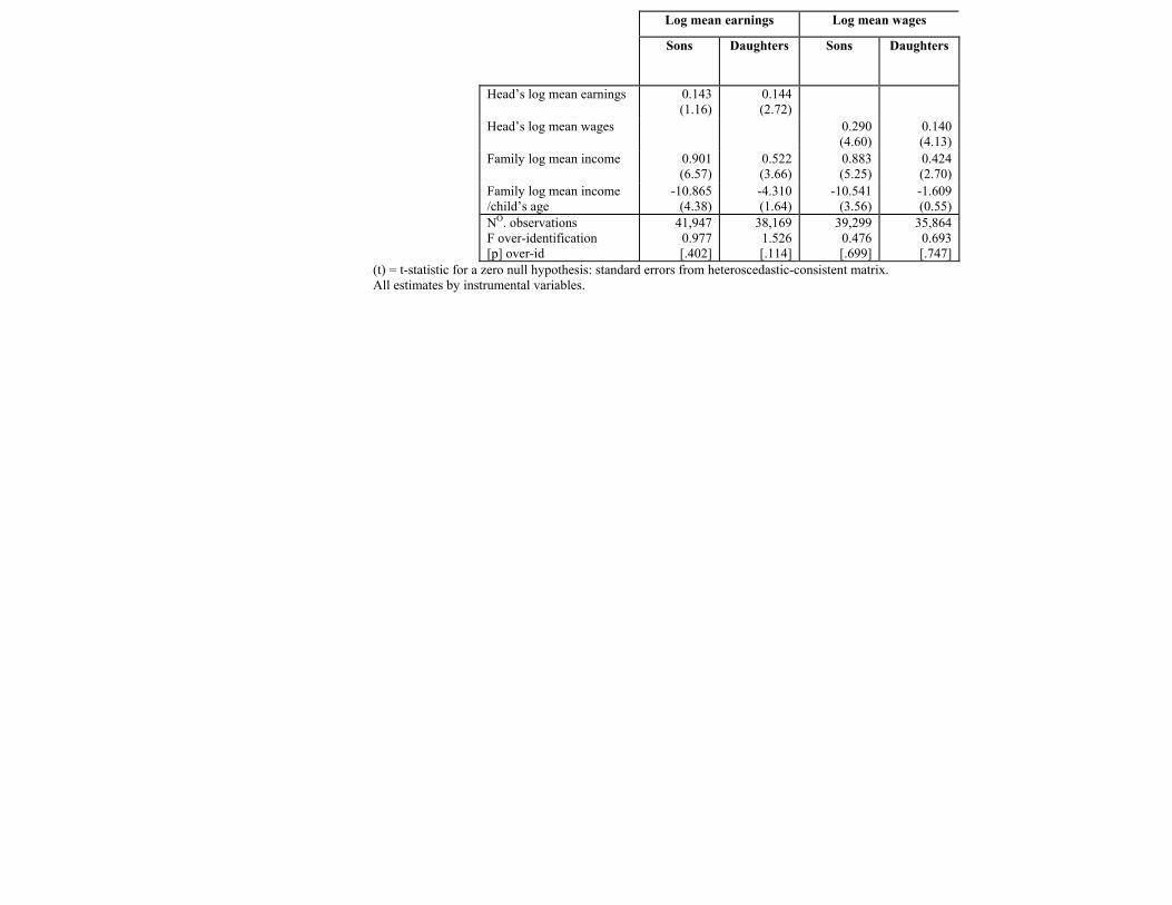
Log mean earnings Log mean wages

Sons Daughters Sons Daughters

Head’s log mean earnings

0.143 (1.16)

0.144(2.72)

Head’s log mean wages

0.290(4.60)

0.140(4.13)

Family log mean income

0.901 (6.57)

0.522(3.66)

0.883(5.25)

0.424(2.70)

Family log mean income /child’s age

-10.865 (4.38)

-4.310(1.64)

-10.541(3.56)

-1.609(0.55)

NO. observations F over-identification [p] over-id

41,947 0.977 [.402]

38,1691.526[.114]

39,2990.476[.699]

35,8640.693[.747]

(t) = t-statistic for a zero null hypothesis: standard errors from heteroscedastic-consistent matrix. All estimates by instrumental variables.