Control Systems

i

About the Tutorial

This tutorial is meant to provide the readers the knowhow of how to analyze the control

systems with the help of mathematical models. After completing this tutorial, you will be

able to learn various methods and techniques in order to improve the performance of the

control systems based on the requirements.

Audience

This tutorial is meant for all those readers who are aspiring to learn the fundamental

concepts of Control Systems.

Prerequisites

A learner who wants to go ahead with this tutorial needs to have a basic understanding of

Signals and Systems.

Copyright & Disclaimer

Copyright 2016 by Tutorials Point (I) Pvt. Ltd.

All the content and graphics published in this e-book are the property of Tutorials Point (I)

Pvt. Ltd. The user of this e-book is prohibited to reuse, retain, copy, distribute or republish

any contents or a part of contents of this e-book in any manner without written consent

of the publisher.

We strive to update the contents of our website and tutorials as timely and as precisely as

possible, however, the contents may contain inaccuracies or errors. Tutorials Point (I) Pvt.

Ltd. provides no guarantee regarding the accuracy, timeliness or completeness of our

website or its contents including this tutorial. If you discover any errors on our website or

in this tutorial, please notify us at contact@tutorialspoint.com.

Control Systems

ii

Table of Contents

About the Tutorial ............................................................................................................................................ i Audience ........................................................................................................................................................... i Prerequisites ..................................................................................................................................................... i Copyright & Disclaimer ..................................................................................................................................... i Table of Contents ............................................................................................................................................ ii

1. Control Systems − Introduction ................................................................................................................. 1 Classification of Control Systems ..................................................................................................................... 1

2. Control Systems − Feedback ..................................................................................................................... 4 Types of Feedback ........................................................................................................................................... 4 Effects of Feedback ......................................................................................................................................... 5

3. Control Systems − Mathematical Models .................................................................................................. 8 Differential Equation Model ............................................................................................................................ 8 Transfer Function Model ................................................................................................................................. 9

4. Control Systems – Modeling of Mechanical Systems ............................................................................... 11 Modeling of Translational Mechanical Systems ............................................................................................ 11 Modeling of Rotational Mechanical Systems ................................................................................................ 13

5. Control Systems – Electrical Analogies of Mechanical Systems ............................................................... 16 Force Voltage Analogy ................................................................................................................................... 16 Force Current Analogy ................................................................................................................................... 18

6. Control Systems − Block Diagrams .......................................................................................................... 20 Basic Elements of Block Diagram ................................................................................................................... 20 Block Diagram Representation of Electrical Systems .................................................................................... 22

7. Control Systems − Block Diagram Algebra ............................................................................................... 25 Basic Connections for Blocks ......................................................................................................................... 25 Block Diagram Algebra for Summing Points .................................................................................................. 27 Block Diagram Algebra for Take-off Points .................................................................................................... 29

8. Control Systems – Block Diagram Reduction ........................................................................................... 32 Block Diagram Reduction Rules ..................................................................................................................... 32

9. Control Systems − Signal Flow Graphs ..................................................................................................... 36 Basic Elements of Signal Flow Graph ............................................................................................................. 36 Construction of Signal Flow Graph ................................................................................................................ 37 Conversion of Block Diagrams into Signal Flow Graphs ................................................................................ 38

10. Control Systems – Mason’s Gain Formula ............................................................................................... 41 Calculation of Transfer Function using Mason’s Gain Formula ..................................................................... 42

11. Control Systems − Time Response Analysis ............................................................................................. 44 What is Time Response?................................................................................................................................ 44 Standard Test Signals ..................................................................................................................................... 45

12. Control Systems – Response of the First Order System ........................................................................... 48

Control Systems

iii

Impulse Response of First Order System ....................................................................................................... 49 Step Response of First Order System ............................................................................................................ 50 Ramp Response of First Order System .......................................................................................................... 51 Parabolic Response of First Order System..................................................................................................... 52

13. Control Systems – Response of Second Order System ............................................................................. 54 Step Response of Second Order System ....................................................................................................... 55 Impulse Response of Second Order System .................................................................................................. 58

14. Control Systems − Time Domain Specifications ....................................................................................... 60 Delay Time ..................................................................................................................................................... 60 Rise Time ....................................................................................................................................................... 61 Peak Time ...................................................................................................................................................... 61 Peak Overshoot ............................................................................................................................................. 62 Settling time .................................................................................................................................................. 63

15. Control Systems − Steady State Errors .................................................................................................... 65 Steady State Errors for Unity Feedback Systems........................................................................................... 65 Steady State Errors for Non-Unity Feedback Systems ................................................................................... 67

16. Control Systems − Stability ..................................................................................................................... 69 What is Stability? ........................................................................................................................................... 69 Types of Systems based on Stability .............................................................................................................. 69

17. Control Systems − Stability Analysis ........................................................................................................ 71 Routh-Hurwitz Stability Criterion .................................................................................................................. 71 Routh Array Method...................................................................................................................................... 71 Special Cases of Routh Array ......................................................................................................................... 73

18. Control Systems − Root Locus ................................................................................................................. 76 Basics of Root Locus ...................................................................................................................................... 76

19. Control Systems – Construction of Root Locus ........................................................................................ 78 Rules for Construction of Root Locus ............................................................................................................ 78

20. Control Systems – Frequency Response Analysis .................................................................................... 82 What is Frequency Response? ....................................................................................................................... 82 Frequency Domain Specifications ................................................................................................................. 83

21. Control Systems − Bode Plots .................................................................................................................. 86 Basics of Bode Plots ....................................................................................................................................... 86

22. Control Systems – Construction of Bode Plots ........................................................................................ 90 Rules for Construction of Bode Plots ............................................................................................................. 90 Stability Analysis using Bode Plots ................................................................................................................ 90

23. Control Systems − Polar Plots.................................................................................................................. 92 Rules for Drawing Polar Plots ........................................................................................................................ 93

24. Control Systems − Nyquist Plots .............................................................................................................. 95 Nyquist Stability Criterion.............................................................................................................................. 95 Rules for Drawing Nyquist Plots .................................................................................................................... 96

Control Systems

iv

Stability Analysis using Nyquist Plots ............................................................................................................ 96

25. Control Systems − Compensators ............................................................................................................ 98 Lag Compensator ........................................................................................................................................... 98 Lead Compensator......................................................................................................................................... 99 Lag-Lead Compensator ................................................................................................................................ 100

26. Control Systems − Controllers ............................................................................................................... 101 Proportional Controller ............................................................................................................................... 101 Derivative Controller ................................................................................................................................... 102 Integral Controller ....................................................................................................................................... 102 Proportional Derivative (PD) Controller ...................................................................................................... 103 Proportional Integral (PI) Controller ............................................................................................................ 104 Proportional Integral Derivative (PID) Controller ........................................................................................ 104

27. Control Systems − State Space Model ................................................................................................... 106 Basic Concepts of State Space Model .......................................................................................................... 106 State Space Model from Differential Equation............................................................................................ 107 State Space Model from Transfer Function ................................................................................................. 108

28. Control Systems − State Space Analysis ................................................................................................ 112 Transfer Function from State Space Model ................................................................................................. 112 State Transition Matrix and its Properties ................................................................................................... 113 Controllability and Observability ................................................................................................................. 114

Control Systems

5

A control system is a system, which provides the desired response by controlling the output. The following figure shows the simple block diagram of a control system.

Here, the control system is represented by a single block. Since, the output is controlled by

varying input, the control system got this name. We will vary this input with some mechanism.

In the next section on open loop and closed loop control systems, we will study in detail about

the blocks inside the control system and how to vary this input in order to get the desired

response.

Examples: Traffic lights control system, washing machine

Traffic lights control system is an example of control system. Here, a sequence of input

signal is applied to this control system and the output is one of the three lights that will be

on for some duration of time. During this time, the other two lights will be off. Based on the

traffic study at a particular junction, the on and off times of the lights can be determined.

Accordingly, the input signal controls the output. So, the traffic lights control system operates

on time basis.

Classification of Control Systems

Based on some parameters, we can classify the control systems into the following ways.

Continuous time and Discrete-time Control Systems

Control Systems can be classified as continuous time control systems and discrete time

control systems based on the type of the signal used.

In continuous time control systems, all the signals are continuous in time. But, in

discrete time control systems, there exists one or more discrete time signals.

SISO and MIMO Control Systems

Control Systems can be classified as SISO control systems and MIMO control systems

based on the number of inputs and outputs present.

1. Control Systems − Introduction

Control Systems

6

SISO (Single Input and Single Output) control systems have one input and one output.

Whereas, MIMO (Multiple Inputs and Multiple Outputs) control systems have more

than one input and more than one output.

Open Loop and Closed Loop Control Systems

Control Systems can be classified as open loop control systems and closed loop control

systems based on the feedback path.

In open loop control systems, output is not fed-back to the input. So, the control action is

independent of the desired output.

The following figure shows the block diagram of the open loop control system.

Here, an input is applied to a controller and it produces an actuating signal or controlling

signal. This signal is given as an input to a plant or process which is to be controlled. So, the

plant produces an output, which is controlled. The traffic lights control system which we

discussed earlier is an example of an open loop control system.

In closed loop control systems, output is fed back to the input. So, the control action is

dependent on the desired output.

The following figure shows the block diagram of negative feedback closed loop control system.

Control Systems

7

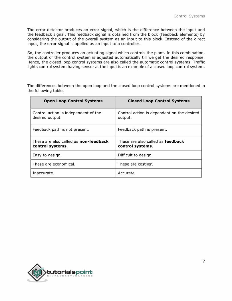
The error detector produces an error signal, which is the difference between the input and

the feedback signal. This feedback signal is obtained from the block (feedback elements) by

considering the output of the overall system as an input to this block. Instead of the direct

input, the error signal is applied as an input to a controller.

So, the controller produces an actuating signal which controls the plant. In this combination,

the output of the control system is adjusted automatically till we get the desired response.

Hence, the closed loop control systems are also called the automatic control systems. Traffic

lights control system having sensor at the input is an example of a closed loop control system.

The differences between the open loop and the closed loop control systems are mentioned in

the following table.

Open Loop Control Systems Closed Loop Control Systems

Control action is independent of the desired output.

Control action is dependent on the desired output.

Feedback path is not present. Feedback path is present.

These are also called as non-feedback

control systems. These are also called as feedback

control systems.

Easy to design. Difficult to design.

These are economical. These are costlier.

Inaccurate. Accurate.

Control Systems

8

If either the output or some part of the output is returned to the input side and utilized as

part of the system input, then it is known as feedback. Feedback plays an important role in

order to improve the performance of the control systems. In this chapter, let us discuss the

types of feedback & effects of feedback.

Types of Feedback

There are two types of feedback:

Positive feedback

Negative feedback

Positive Feedback

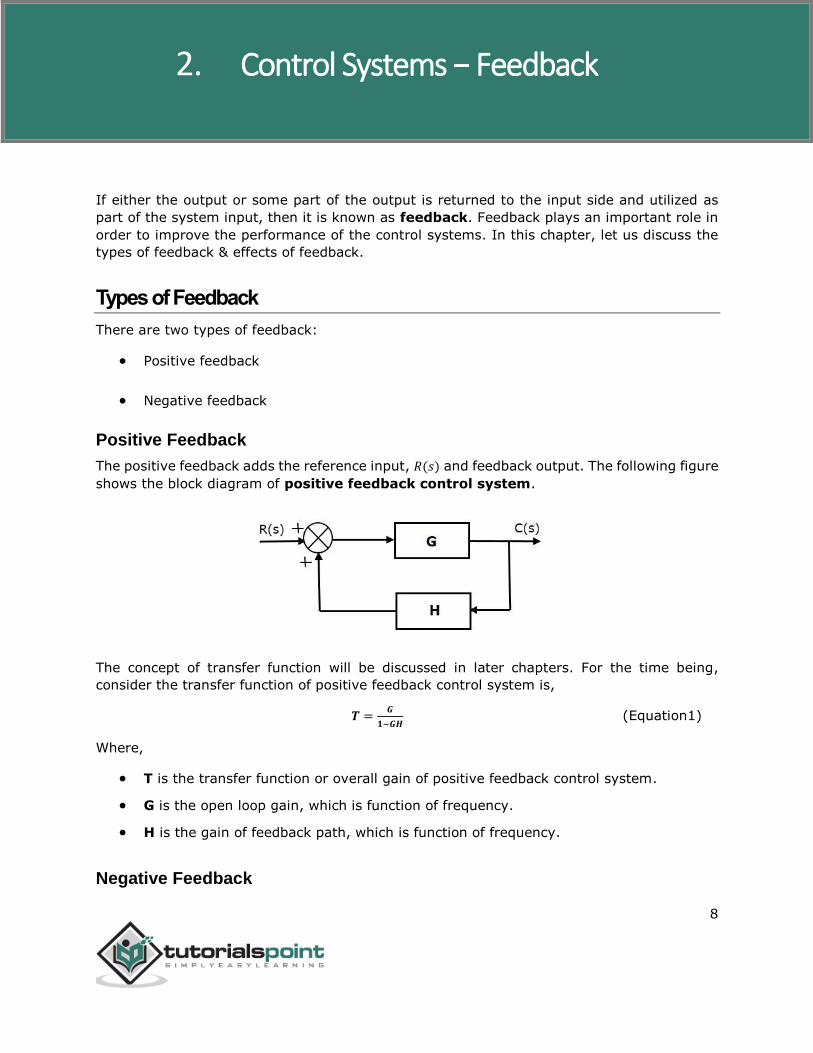
The positive feedback adds the reference input, 𝑅(𝑠) and feedback output. The following figure

shows the block diagram of positive feedback control system.

The concept of transfer function will be discussed in later chapters. For the time being,

consider the transfer function of positive feedback control system is,

𝑻 =𝑮

𝟏−𝑮𝑯 (Equation1)

Where,

T is the transfer function or overall gain of positive feedback control system.

G is the open loop gain, which is function of frequency.

H is the gain of feedback path, which is function of frequency.

Negative Feedback

2. Control Systems − Feedback

Control Systems

9

Negative feedback reduces the error between the reference input, 𝑅(𝑠) and system output.

The following figure shows the block diagram of the negative feedback control system.

Transfer function of negative feedback control system is,

𝑻 =𝑮

𝟏+𝑮𝑯 (Equation 2)

Where,

T is the transfer function or overall gain of negative feedback control system

G is the open loop gain, which is function of frequency

H is the gain of feedback path, which is function of frequency

The derivation of the above transfer function is present in later chapters.

Effects of Feedback

Let us now understand the effects of feedback.

Effect of Feedback on Overall Gain

From Equation 2, we can say that the overall gain of negative feedback closed loop

control system is the ratio of ‘G’ and (1+GH). So, the overall gain may increase or

decrease depending on the value of (1+GH).

If the value of (1+GH) is less than 1, then the overall gain increases. In this case, ‘GH’

value is negative because the gain of the feedback path is negative.

If the value of (1+GH) is greater than 1, then the overall gain decreases. In this case,

‘GH’ value is positive because the gain of the feedback path is positive.

In general, ‘G’ and ‘H’ are functions of frequency. So, the feedback will increase the overall gain of the system in one frequency range and decrease in the other frequency range.

Control Systems

10

Effect of Feedback on Sensitivity

Sensitivity of the overall gain of negative feedback closed loop control system (T) to the variation in open loop gain (G) is defined as

𝐒𝐆𝐓 =

𝛛𝐓𝐓⁄

𝛛𝐆𝐆⁄

=𝐏𝐞𝐫𝐜𝐞𝐧𝐭𝐚𝐠𝐞 𝐜𝐡𝐚𝐧𝐠𝐞 𝐢𝐧 𝐓

𝐏𝐞𝐫𝐜𝐞𝐧𝐭𝐚𝐠𝐞 𝐜𝐡𝐚𝐧𝐠𝐞 𝐢𝐧 𝐆 (Equation 3)

Where, 𝞉T is the incremental change in T due to incremental change in G.

We can rewrite Equation 3 as

𝑺𝑮𝑻 =

𝝏𝑻

𝝏𝑮 𝑮

𝑻 (Equation 4)

Do partial differentiation with respect to G on both sides of Equation 2.

∂T

∂G=

∂

∂G(

G

1+GH) =

(1+GH).1−𝐺(𝐻)

(1+GH)2 =1

(1+GH)2 (Equation 5)

From Equation 2, you will get

𝐺

𝑇= 1 + 𝐺𝐻 (Equation 6)

Substitute Equation 5 and Equation 6 in Equation 4.

𝑆𝐺𝑇 =

1

(1 + GH)2(1 + 𝐺𝐻) =

1

1 + 𝐺𝐻

So, we got the sensitivity of the overall gain of closed loop control system as the reciprocal of (1+GH). So, Sensitivity may increase or decrease depending on the value of (1+GH).

If the value of (1+GH) is less than 1, then sensitivity increases. In this case, ‘GH’ value

is negative because the gain of feedback path is negative.

If the value of (1+GH) is greater than 1, then sensitivity decreases. In this case, ‘GH’

value is positive because the gain of feedback path is positive.

In general, ‘G’ and ‘H’ are functions of frequency. So, feedback will increase the sensitivity of

the system gain in one frequency range and decrease in the other frequency range. Therefore,

we have to choose the values of ‘GH’ in such a way that the system is insensitive or less sensitive to parameter variations.

Effect of Feedback on Stability

A system is said to be stable, if its output is under control. Otherwise, it is said to be

unstable.

In Equation 2, if the denominator value is zero (i.e., GH = -1), then the output of the

control system will be infinite. So, the control system becomes unstable.

Control Systems

11

Therefore, we have to properly choose the feedback in order to make the control system stable.

Effect of Feedback on Noise

To know the effect of feedback on noise, let us compare the transfer function relations with and without feedback due to noise signal alone.

Consider an open loop control system with noise signal as shown below.

The open loop transfer function due to noise signal alone is

𝐶(𝑠)

𝑁(𝑠)= 𝐺𝑏 (Equation 7)

It is obtained by making the other input 𝑅(𝑠) equal to zero.

Consider a closed loop control system with noise signal as shown below.

The closed loop transfer function due to noise signal alone is

𝐶(𝑠)

𝑁(𝑠)=

𝐺𝑏

1+𝐺𝑎𝐺𝑏𝐻 (Equation 8)

It is obtained by making the other input 𝑅(𝑠) equal to zero.

Compare Equation 7 and Equation 8,

In the closed loop control system, the gain due to noise signal is decreased by a factor of (1 + 𝐺𝑎𝐺𝑏𝐻) provided that the term (1 + 𝐺𝑎𝐺𝑏𝐻) is greater than one.

Control Systems

12

The control systems can be represented with a set of mathematical equations known as

mathematical model. These models are useful for analysis and design of control systems.

Analysis of control system means finding the output when we know the input and

mathematical model. Design of control system means finding the mathematical model when

we know the input and the output.

The following mathematical models are mostly used.

Differential equation model

Transfer function model

State space model

Let us discuss the first two models in this chapter.

Differential Equation Model

Differential equation model is a time domain mathematical model of control systems. Follow

these steps for differential equation model.

Apply basic laws to the given control system.

Get the differential equation in terms of input and output by eliminating the

intermediate variable(s).

Example

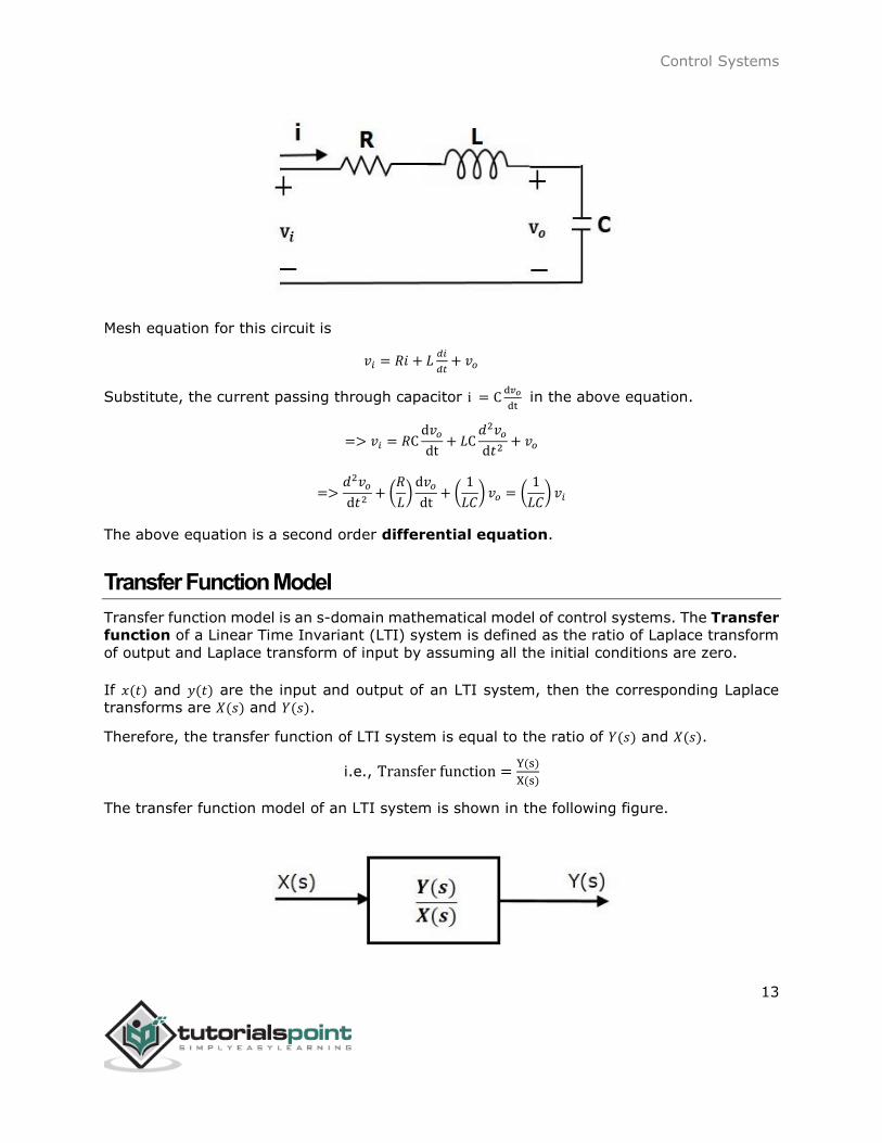
Consider the following electrical system as shown in the following figure. This circuit consists

of resistor, inductor and capacitor. All these electrical elements are connected in series. The input voltage applied to this circuit is 𝑣𝑖 and the voltage across the capacitor is the output

voltage 𝑣𝑜.

3. Control Systems − Mathematical Models

Control Systems

13

Mesh equation for this circuit is

𝑣𝑖 = 𝑅𝑖 + 𝐿𝑑𝑖

𝑑𝑡+ 𝑣𝑜

Substitute, the current passing through capacitor i = Cd𝑣𝑜

dt in the above equation.

=> 𝑣𝑖 = 𝑅Cd𝑣𝑜

dt+ 𝐿C

𝑑2𝑣𝑜

d𝑡2+ 𝑣𝑜

=>𝑑2𝑣𝑜

d𝑡2+ (

𝑅

𝐿)

d𝑣𝑜

dt+ (

1

𝐿𝐶) 𝑣𝑜 = (

1

𝐿𝐶) 𝑣𝑖

The above equation is a second order differential equation.

Transfer Function Model

Transfer function model is an s-domain mathematical model of control systems. The Transfer

function of a Linear Time Invariant (LTI) system is defined as the ratio of Laplace transform

of output and Laplace transform of input by assuming all the initial conditions are zero. If 𝑥(𝑡) and 𝑦(𝑡) are the input and output of an LTI system, then the corresponding Laplace

transforms are 𝑋(𝑠) and 𝑌(𝑠).

Therefore, the transfer function of LTI system is equal to the ratio of 𝑌(𝑠) and 𝑋(𝑠).

i.e., Transfer function =Y(s)

X(s)

The transfer function model of an LTI system is shown in the following figure.

Control Systems

14

Here, we represented an LTI system with a block having transfer function inside it. And this block has an input 𝑋(𝑠) & output 𝑌(𝑠).

Example

Previously, we got the differential equation of an electrical system as

𝑑2𝑣𝑜

d𝑡2+ (

𝑅

𝐿)

d𝑣𝑜

dt+ (

1

𝐿𝐶) 𝑣𝑜 = (

1

𝐿𝐶) 𝑣𝑖

Apply Laplace transform on both sides.

𝑠2𝑉𝑜(𝑠) + (𝑠𝑅

𝐿) 𝑉𝑜(𝑠) + (

1

𝐿𝐶) 𝑉𝑜(𝑠) = (

1

𝐿𝐶) 𝑉𝑖(𝑠)

=> {𝑠2 + (𝑅

𝐿) 𝑠 +

1

𝐿𝐶} 𝑉𝑜(𝑠) = (

1

𝐿𝐶) 𝑉𝑖(𝑠)

=>𝑉𝑜(𝑠)

𝑉𝑖(𝑠)=

1 𝐿𝐶⁄

𝑠2 + (𝑅𝐿

) 𝑠 +1

𝐿𝐶

Where,

𝑉𝑖(𝑠) is the Laplace transform of the input voltage 𝑣𝑖

𝑉𝑜(𝑠) is the Laplace transform of the output voltage 𝑣𝑜

The above equation is a transfer function of the second order electrical system. The transfer

function model of this system is shown below.

Here, we show a second order electrical system with a block having the transfer function inside it. And this block has an input 𝑉𝑖(𝑠) & an output 𝑉𝑜(𝑠).

Control Systems

15

In this chapter, let us discuss the differential equation modeling of mechanical systems. There are two types of mechanical systems based on the type of motion.

Translational mechanical systems

Rotational mechanical systems

Modeling of Translational Mechanical Systems

Translational mechanical systems move along a straight line. These systems mainly consist

of three basic elements. Those are mass, spring and dashpot or damper.

If a force is applied to a translational mechanical system, then it is opposed by opposing

forces due to mass, elasticity and friction of the system. Since the applied force and the

opposing forces are in opposite directions, the algebraic sum of the forces acting on the

system is zero. Let us now see the force opposed by these three elements individually.

Mass

Mass is the property of a body, which stores kinetic energy. If a force is applied on a body

having mass M, then it is opposed by an opposing force due to mass. This opposing force is proportional to the acceleration of the body. Assume elasticity and friction are negligible.

𝐹𝑚 ∝ 𝑎

=> 𝐹𝑚 = 𝑀𝑎 = 𝑀𝑑2𝑥

𝑑𝑡2

𝐹 = 𝐹𝑚 = 𝑀𝑑2𝑥

𝑑𝑡2

Where,

𝑭 is the applied force

𝑭𝒎 is the opposing force due to mass

4. Control Systems – Modeling of Mechanical Systems

Control Systems

16

𝑴 is mass

𝒂 is acceleration

𝒙 is displacement

Spring

Spring is an element, which stores potential energy. If a force is applied on spring K, then

it is opposed by an opposing force due to elasticity of spring. This opposing force is

proportional to the displacement of the spring. Assume mass and friction are negligible.

𝐹𝑘 ∝ 𝑥

=> 𝐹𝑘 = 𝐾𝑥

𝐹 = 𝐹𝑘 = 𝐾𝑥

Where,

𝑭 is the applied force

𝑭𝒌 is the opposing force due to elasticity of spring

𝑲 is spring constant

𝒙 is displacement

Dashpot

If a force is applied on dashpot B, then it is opposed by an opposing force due to friction of

the dashpot. This opposing force is proportional to the velocity of the body. Assume mass and elasticity are negligible.

Control Systems

17

𝐹𝑏 ∝ 𝑣

=> 𝐹𝑏 = 𝐵𝑣 = 𝐵𝑑𝑥

𝑑𝑡

𝐹 = 𝐹𝑏 = 𝐵𝑑𝑥

𝑑𝑡

Where,

𝑭𝒃 is the opposing force due to friction of dashpot

𝑩 is the frictional coefficient

𝒗 is velocity

𝒙 is displacement

Modeling of Rotational Mechanical Systems

Rotational mechanical systems move about a fixed axis. These systems mainly consist of three basic elements. Those are moment of inertia, torsional spring and dashpot.

If a torque is applied to a rotational mechanical system, then it is opposed by opposing torques

due to moment of inertia, elasticity and friction of the system. Since the applied torque and

the opposing torques are in opposite directions, the algebraic sum of torques acting on the system is zero. Let us now see the torque opposed by these three elements individually.

Moment of Inertia

In translational mechanical system, mass stores kinetic energy. Similarly, in rotational

mechanical system, moment of inertia stores kinetic energy.

If a torque is applied on a body having moment of inertia J, then it is opposed by an opposing

torque due to the moment of inertia. This opposing torque is proportional to angular acceleration of the body. Assume elasticity and friction are negligible.

Control Systems

18

𝑇𝑗 ∝ 𝛼

=> 𝑇𝑗 = 𝐽𝛼 = 𝐽𝑑2𝜃

𝑑𝑡2

𝑇 = 𝑇𝑗 = 𝐽𝑑2𝜃

𝑑𝑡2

Where,

𝑻 is the applied torque

𝑻𝒋 is the opposing torque due to moment of inertia

𝑱 is moment of inertia

𝛂 is angular acceleration

𝛉 is angular displacement.

Torsional Spring

In translational mechanical system, spring stores potential energy. Similarly, in rotational

mechanical system, torsional spring stores potential energy.

If a torque is applied on torsional spring K, then it is opposed by an opposing torque due to

the elasticity of torsional spring. This opposing torque is proportional to the angular

displacement of the torsional spring. Assume that the moment of inertia and friction are negligible.

Control Systems

19

𝑇𝑘 ∝ 𝜃

=> 𝑇𝑘 = 𝐾𝜃

𝑇 = 𝑇𝑘 = 𝐾𝜃

Where,

𝑻 is the applied torque

𝑻𝒌 is the opposing torque due to elasticity of torsional spring

𝑲 is the torsional spring constant

𝛉 is angular displacement

Dashpot

If a torque is applied on dashpot B, then it is opposed by an opposing torque due to the

rotational friction of the dashpot. This opposing torque is proportional to the angular velocity of the body. Assume the moment of inertia and elasticity are negligible.

𝑇𝑏 ∝ 𝜔

=> 𝑇𝑏 = 𝐵𝜔 = 𝐵𝑑𝜃

𝑑𝑡

𝑇 = 𝑇𝑏 = 𝐵𝑑𝜃

𝑑𝑡

Control Systems

20

Where,

𝑻𝒃 is the opposing torque due to the rotational friction of the dashpot

𝑩 is the rotational friction coefficient

𝛚 is the angular velocity

𝛉 is the angular displacement.

Control Systems

21

Two systems are said to be analogous to each other if the following two conditions are satisfied.

The two systems are physically different

Differential equation modelling of these two systems are same

Electrical systems and mechanical systems are two physically different systems. There are

two types of electrical analogies of translational mechanical systems. Those are force voltage

analogy and force current analogy.

Force Voltage Analogy

In force voltage analogy, the mathematical equations of translational mechanical system are compared with mesh equations of the electrical system.

Consider the following translational mechanical system as shown in the following figure.

The force balanced equation for this system is

𝐹 = 𝐹𝑚 + 𝐹𝑏+𝐹𝑘

=> 𝐹 = 𝑀𝑑2𝑥

𝑑𝑡2 + 𝐵𝑑𝑥

𝑑𝑡+ 𝑘𝑥 (Equation 1)

Consider the following electrical system as shown in the following figure. This circuit consists

of a resistor, an inductor and a capacitor. All these electrical elements are connected in a series. The input voltage applied to this circuit is 𝑉 volts and the current flowing through the

circuit is 𝑖 Amps.

5. Control Systems – Electrical Analogies of Mechanical Systems

Control Systems

22

Mesh equation for this circuit is -

𝑉 = 𝑅𝑖 + 𝐿𝑑𝑖

𝑑𝑡+

1

𝐶∫ 𝑖𝑑𝑡 (Equation 2)

Substitute, i = dq

dt in Equation 2.

𝑉 = 𝑅dq

dt+ 𝐿

𝑑2𝑞

𝑑𝑡2+

𝑞

𝐶

=> 𝑉 = 𝐿𝑑2𝑞

𝑑𝑡2 + 𝑅dq

dt+ (

1

𝐶) 𝑞 (Equation 3)

By comparing Equation 1 and Equation 3, we will get the analogous quantities of the

translational mechanical system and electrical system. The following table shows these analogous quantities.

Translational Mechanical System Electrical System

Force (F) Voltage (V)

Mass (M) Inductance (L)

Frictional coefficient (B) Resistance (R)

Spring constant (K) Reciprocal of Capacitance (1

𝐶)

Displacement (x) Charge (q)

Velocity (v) Current (i)

Similarly, there is torque voltage analogy for rotational mechanical systems. Let us now

discuss about this analogy.

Torque Voltage Analogy

In this analogy, the mathematical equations of rotational mechanical system are compared with mesh equations of the electrical system.

Rotational mechanical system is shown in the following figure.

Control Systems

23

The torque balanced equation is -

𝑇 = 𝑇𝑗 + 𝑇𝑏+𝑇𝑘

=> 𝑇 = 𝐽𝑑2𝜃

𝑑𝑡2 + 𝐵𝑑𝜃

𝑑𝑡+ 𝑘𝜃 (Equation 4)

By comparing Equation 4 and Equation 3, we will get the analogous quantities of rotational

mechanical system and electrical system. The following table shows these analogous

quantities.

Rotational Mechanical System Electrical System

Torque (T) Voltage (V)

Moment of Inertia (J) Inductance (L)

Rotational friction coefficient (B) Resistance (R)

Torsional spring constant (K) Reciprocal of Capacitance (1

𝐶)

Angular Displacement (𝜃) Charge (q)

Angular Velocity (𝜔) Current (i)

Force Current Analogy

In force current analogy, the mathematical equations of the translational mechanical system are compared with the nodal equations of the electrical system.

Consider the following electrical system as shown in the following figure. This circuit consists

of current source, resistor, inductor and capacitor. All these electrical elements are connected in parallel.

Control Systems

24

The nodal equation is -

i =𝑉

𝑅+

1

𝐿∫ V dt + C

dV

dt (Equation 5)

Substitute, 𝑉 =𝑑𝛹

𝑑𝑡 in Equation 5.

i =1

𝑅

𝑑𝛹

𝑑𝑡+ (

1

𝐿) 𝛹 + C

𝑑2𝛹

𝑑𝑡2

=> i = C𝑑2𝛹

𝑑𝑡2 + (1

𝑅)

𝑑𝛹

𝑑𝑡+ (

1

𝐿) 𝛹 (Equation 6)

By comparing Equation 1 and Equation 6, we will get the analogous quantities of the

translational mechanical system and electrical system. The following table shows these

analogous quantities.

Translational Mechanical System Electrical System

Force (F) Current (i)

Mass (M) Capacitance (C)

Frictional coefficient (B) Reciprocal of Resistance (1

𝑅)

Spring constant (K) Reciprocal of Inductance (1

𝐿)

Displacement (x) Magnetic Flux (𝛹)

Velocity (v) Voltage (V)

Similarly, there is a torque current analogy for rotational mechanical systems. Let us now

discuss this analogy.

Torque Current Analogy

In this analogy, the mathematical equations of the rotational mechanical system are compared with the nodal mesh equations of the electrical system.

Control Systems

25

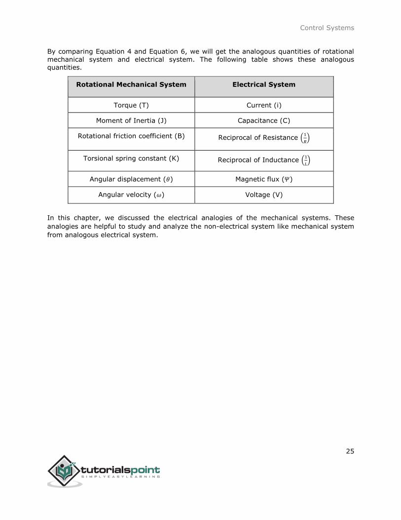
By comparing Equation 4 and Equation 6, we will get the analogous quantities of rotational

mechanical system and electrical system. The following table shows these analogous

quantities.

Rotational Mechanical System Electrical System

Torque (T) Current (i)

Moment of Inertia (J) Capacitance (C)

Rotational friction coefficient (B) Reciprocal of Resistance (1

𝑅)

Torsional spring constant (K) Reciprocal of Inductance (1

𝐿)

Angular displacement (𝜃) Magnetic flux (𝛹)

Angular velocity (𝜔) Voltage (V)

In this chapter, we discussed the electrical analogies of the mechanical systems. These

analogies are helpful to study and analyze the non-electrical system like mechanical system

from analogous electrical system.

Control Systems

26

Block diagrams consist of a single block or a combination of blocks. These are used to

represent the control systems in pictorial form.

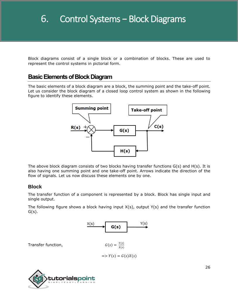
Basic Elements of Block Diagram

The basic elements of a block diagram are a block, the summing point and the take-off point.

Let us consider the block diagram of a closed loop control system as shown in the following figure to identify these elements.

The above block diagram consists of two blocks having transfer functions G(s) and H(s). It is

also having one summing point and one take-off point. Arrows indicate the direction of the

flow of signals. Let us now discuss these elements one by one.

Block

The transfer function of a component is represented by a block. Block has single input and single output.

The following figure shows a block having input X(s), output Y(s) and the transfer function G(s).

Transfer function, 𝐺(𝑠) = 𝑌(𝑠)

𝑋(𝑠)

=> 𝑌(𝑠) = 𝐺(𝑠)𝑋(𝑠)

6. Control Systems − Block Diagrams

Control Systems

27

Output of the block is obtained by multiplying transfer function of the block with input.

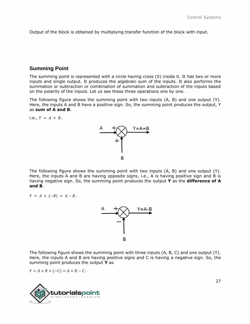
Summing Point

The summing point is represented with a circle having cross (X) inside it. It has two or more

inputs and single output. It produces the algebraic sum of the inputs. It also performs the

summation or subtraction or combination of summation and subtraction of the inputs based on the polarity of the inputs. Let us see these three operations one by one.

The following figure shows the summing point with two inputs (A, B) and one output (Y).

Here, the inputs A and B have a positive sign. So, the summing point produces the output, Y as sum of A and B.

i.e., 𝑌 = 𝐴 + 𝐵.

The following figure shows the summing point with two inputs (A, B) and one output (Y).

Here, the inputs A and B are having opposite signs, i.e., A is having positive sign and B is

having negative sign. So, the summing point produces the output Y as the difference of A

and B.

𝑌 = 𝐴 + (−𝐵) = 𝐴 − 𝐵.

The following figure shows the summing point with three inputs (A, B, C) and one output (Y).

Here, the inputs A and B are having positive signs and C is having a negative sign. So, the summing point produces the output Y as

𝑌 = 𝐴 + 𝐵 + (−𝐶) = 𝐴 + 𝐵 − 𝐶.

Control Systems

28

Take-off Point

The take-off point is a point from which the same input signal can be passed through more

than one branch. That means with the help of take-off point, we can apply the same input to one or more blocks, summing points.

In the following figure, the take-off point is used to connect the same input, R(s) to two more blocks.

In the following figure, the take-off point is used to connect the output 𝐶(𝑠), as one of the

inputs to the summing point.

Control Systems

29

Block Diagram Representation of Electrical Systems

In this section, let us represent an electrical system with a block diagram. Electrical systems

contain mainly three basic elements — resistor, inductor and capacitor.

Consider a series of RLC circuit as shown in the following figure. Where, 𝑉𝑖(t) and 𝑉𝑜(t) are the

input and output voltages. Let 𝑖(𝑡) be the current passing through the circuit. This circuit is in

time domain.

By applying the Laplace transform to this circuit, will get the circuit in s-domain. The circuit

is as shown in the following figure.

From the above circuit, we can write –

𝐼(𝑠) =𝑉𝑖(𝑠) − 𝑉𝑜(𝑠)

𝑅 + 𝑠𝐿

Control Systems

30

=> 𝐼(𝑠) = {1

𝑅+𝑠𝐿} {𝑉𝑖(𝑠) − 𝑉𝑜(𝑠)} (Equation 1)

𝑉𝑜(𝑠) = (1

𝑠𝐶) 𝐼(𝑠) (Equation 2)

Let us now draw the block diagrams for these two equations individually. And then combine

those block diagrams properly in order to get the overall block diagram of series of RLC Circuit (s-domain).

Equation 1 can be implemented with a block having the transfer function, 1

𝑅+𝑠𝐿. The input and

output of this block are {𝑉𝑖(𝑠) − 𝑉𝑜(𝑠)} and 𝐼(𝑠). We require a summing point to get {𝑉𝑖(𝑠) − 𝑉𝑜(𝑠)}. The block diagram of Equation 1 is shown in the following figure.

Equation 2 can be implemented with a block having transfer function, 1

𝑠𝐶. The input and output

of this block are 𝐼(𝑠) and 𝑉𝑜(𝑠). The block diagram of Equation 2 is shown in the following

figure.

The overall block diagram of the series of RLC Circuit (s-domain) is shown in the following figure.

Control Systems

31

Similarly, you can draw the block diagram of any electrical circuit or system just by following

this simple procedure.

Convert the time domain electrical circuit into an s-domain electrical circuit by applying

Laplace transform.

Write down the equations for the current passing through all series branch elements

and voltage across all shunt branches.

Draw the block diagrams for all the above equations individually.

Combine all these block diagrams properly in order to get the overall block diagram of

the electrical circuit (s-domain).

Control Systems

32

End of ebook preview

If you liked what you saw…

Buy it from our store @ https://store.tutorialspoint.com