absolute and relative deprivation - lakehead...

Absolute and Relative Deprivationand the Measurement of Poverty

by

Jean-Yves DuclosDepartment of Economics and CREFA, Universite Laval, Canada

and UNSW, Sydney, Australia

and

Philippe GregoireCREFA, Universite Laval, Canada

and Department of Economics, University of Western Ontario, Canada

Abstract

This paper develops the link between poverty and inequality by focussingon a class of poverty indices (some of them well-known) which aggregatenormative concerns for absolute and relative deprivation. The indices aredistinguished by a parameter value that captures the ethical sensitivity ofpoverty measurement to “exclusion” or “relative-deprivation” aversion. Theindices can be readily used to predict the impact of growth on poverty. Anillustration using LIS data finds that the United States show more relative de-privation than Denmark and Belgium whatever the percentiles considered,but that overall deprivation comparisons of the four countries consideredwill generally depend on the intensity of the ethical concern for relative de-privation. The impact of growth on poverty also depends on the presence ofand on the attention granted to concerns over relative deprivation.

Keywords Poverty, relative deprivation, inequality, poverty alleviation.

JEL numbers D6, I3, O1.

This research was supported, in part, by grants from the Social Sciences andHumanities Research Council of Canada and from the Fonds FCAR of theProvince of Quebec. The hospitality of the Institut d’Analisi Economica(CSIC) at the Universitat Autonoma de Barcelona (where this paper wasrevised) is also gratefully acknowledged. We further wish to thank GordonAnderson, Michael Hoy, Kuan Xu and two anonymous referees for theiruseful comments.

Corresponding address: Jean-Yves Duclos, Departement d’economique,Pavillon de Seve, Universite Laval, Quebec, Canada, G1K 7P4; Tel.: (418)656-7096; Fax: (418) 656-7798; Email: [email protected]

April, 2002

1 Introduction

Since the work of Sen (1976), taking into account inequality among the

poor, and not solely the incidence or average intensity of poverty, has be-

come common scientific practice and has generated a considerable literature

1. Alongside this has grown a belief among several researchers and policy

analysts that concerns of relativity are also important in assessing poverty

lines. In the words of Townsend (1979), a well-known proponent of that

relativist view:

Individuals, families and groups in the population can be said

to be in poverty when they lack the resources to obtain the type

of diet, participate in the activities and have the living condi-

tions and amenities which are customary, or are at least widely

encouraged or approved, in the societies to which they belong.

Their resources are so seriously below those commanded by the

average individual or family that they are, in effect, excluded

from ordinary living patterns, customs and activities. (p.31)

The link between poverty and relative exclusion from society also tran-

spires from the official use of the concept of social exclusion in the European

Commission, where it is defined “in relation to the social rights of citizens

(...) to participation in the major social and occupational opportunities of

the society.” (Room (1992), p.14) On his part, Sen believes that comparing

poverty across distributions may involve “different standards of minimum

necessities” (1981, p.21) and “that absolutedeprivation in terms of a per-

son’s capabilities relates to relativedeprivation in terms of commodities,

incomes and resources” (1984, p.326). This view is somewhat supported by

the large number of cross-country comparisons using proportions of median

1

or mean incomes as poverty lines.

Another link between poverty and relativity is the frequent normaliza-

tion of poverty indices by possibly different poverty lines (see, for instance,

Foster et al. (1984)), which typically leads to “relative poverty indices” as

defined in Blackorby and Donaldson (1980). Foster and Shorrocks (1988),

Foster and Sen (1997) and Davidson and Duclos (2000) show how such

normalization links relative poverty and relative inequality comparisons. Fi-

nally, having identified the poor and measured the respective intensity of

their poverty, individual poverty is usually aggregated into global poverty

indices, and “in the ’aggregation’ exercise the magnitudes of absolute depri-

vation may have to be supplemented by considerations of relative depriva-

tion” (Sen (1981),p.32).

Among all these links between poverty, inequality and exclusion, it is on

the one between poverty and relative deprivation in the latter “aggregation

exercise” that we wish to focus particularly in this paper2. We will do this by

interpreting a class of poverty indices which combine concerns of absolute

deprivation and of relative deprivation. Absolute deprivation is undoubtedly

“an irreducible core (...) in our idea of poverty, which translates reports of

starvation, malnutrition and visible hardship onto a diagnosis of poverty”

(Sen (1981), p.17). Although sometimes neglected by economists, relative

deprivation has been linked to “definable and measurable social and psycho-

logical reactions, such as different types of alienation” (Durant and Christian

(1990), p.210) by social psychologists and to social protests, discrimination,

feelings of injustice and subjective ill-being (Olson (1986)). It has also been

used to interpret measures of inequality and income redistribution (see for

instance Yitzhaki (1979) and Duclos (2000)).

2

The class of poverty indices we consider in this paper is a generalization

of the Sen(1976)-Thon(1979)- Chakravarty(1983)-Shorrocks(1995) indices

of poverty. The indicesS(v) depend upon an ethical parameterv which

captures the sensitivity of poverty measurement to “exclusion” or “relative-

deprivation” aversion. The greater the value ofv, the greater the weight

assigned to relative deprivation as against absolute deprivation in measuring

and comparing poverty.

The next section sets up the basic definitions and shows the link between

generalized Gini indices and relative deprivation, upon which our subse-

quent work draws. Section 2 then shows how our class of poverty indices

can be understood as a weighted sum of absolute and relative deprivation.

It further points to the indices’ useful and simple graphical interpretation as

weighted areas underneath cumulative poverty gap (CPG) curves, and indi-

cates how they can be used to assess the impact of growth on poverty and

for decomposition analyses. Section 2 also compares the properties of the

S(v) indices with those of additive poverty indices (most saliently, with the

popular class of FGT indices (Foster, Greer and Thorbecke (1984))).

Section 3 illustrates some of the results using Luxembourg Income Study

data drawn from 4 countries. For a reasonable common poverty line, we find

that, whatever the percentiles considered, the United States have more rela-

tive deprivation than Denmark and Belgium, but that the relative deprivation

curve for Italy crosses that of the three other countries. Moreover, for all

but one of the six possible country comparisons, it is not possible to make

unambiguous robust poverty orderings based on CPG curves. Since abso-

lute deprivation and mean poverty are very similar in the four countries, we

thus find that unambiguous poverty comparisons would inevitably depend

on the importance granted to concerns over relative deprivation. The im-

3

pact of growth on poverty is also seen to depend on the presence of and on

concerns for relative deprivation: in pairwise comparisons, poverty is least

responsive to growth in the US and in Denmark, which is also where relative

deprivation is the greatest. The last section concludes our paper.

2 Inequality and relative deprivation

Consider the cumulative distribution of incomeF with support contained in

the nonnegative real line. Let a poverty line be denoted byz, and define

the headcount index asH = F (z). Denote byy∗(p) the quantile function

associated toF . y∗(p) is formally defined asy∗(p) = inf{s ≥ 0|F (s) ≥ p}for p ∈ [0, 1]. For a continuous and strictly increasing distribution,y∗(p) is

simplyF−1(p) and can be thought of as the income of the individual whose

rank (or percentile) isp. Let y(p) be the incomey∗(p) when censored atz,

with y(p) = min(y∗(p), z), and denote the poverty gap of an individual at

rankp by g(p) = (z − y(p)). Note therefore thatg(p) = 0 for p ≥ H. 3

The next most popular poverty index after the headcount is traditionally

denoted byHI, the average poverty gap in the population:

HI =∫ 1

0g(p)dp. (1)

Hence, if perfect targeting of the poor were possible,HI would give

theper capitaexpenditures which the state would need to spend in order to

eradicate poverty completely. Clearly, and as we will discuss more later,HI

does not give any ethical or normative weight to inequality in the distribution

of the poverty gaps.

Let the cumulative poverty gap (CPG) curve be defined as:

G(p) =∫ p

0g(s)ds. (2)

4

This curve was introduced by Jenkins and Lambert (1997), who called

it a ”TIP” curve, and subsequently by Shorrocks (1998), who labelled it a

”Poverty Profile” curve (see also on this the work by Spencer and Fisher

(1992)). It is clear from (2) that :

dG(p)dp

= g(p). (3)

By definition, we have thatG(0) = 0 andG(p) = HI for p ≥ H. G(p)

thus becomes saturated atp = H. G(p)/p is the average poverty gap of

the100 · p% poorest members of the population.G(H)/H is the average

poverty gap of the poor, often defined in the literature (see Sen (1976)) asI.

The CPG curve is continuous, non-decreasing and concave inp, as we

can see on Figure 1, where CPG curvesGA(p) andGB(p) have been drawn

for two hypothetical distributions,A andB. The headcounts,HA andHB,

are given by the values ofp at which the curves flatten out. The slope ofG(p)

represents the poverty gap at percentilep, and the peak of a CPG curve yields

the average poverty gap. As we shall see,the curvature of the CPG curve also

shows the extent of inequality in the distribution of the poverty gaps.

”place Figure 1 here”

As can be seen on the Figure,A has everywhere a greater cumulative

poverty gap whatever the percentage of the poorest part of the population

considered.A has also more inequality among its poor thanB (for which

all poor have the same incomes, as can be seen from the initial straight line

segment).A has nevertheless a lower headcount thanB. In determining

which of A or B has more poverty, there may therefore exist a trade-off

between the number of the poor (the “incidence” of povertyH), the overall

average poverty gap (the average “intensity”,HI), and the inequality in

poverty (the curvature ofG(p)).

5

The class of poverty indicesS(v) on which we will focus in this paper

will all indicate that poverty is greater inA than inB (although the head-

count index clearly would not). This is becauseGA(p) is everywhere greater

thanGB(p). This ordering of poverty in terms of CPG curves is in fact valid

for a broader class of poverty indices thanS(v), as shown in Jenkins and

Lambert (1997) and in Shorrocks (1998). LetΠ be the class of poverty in-

dicesπ that are replication invariant, increasing and Schur-convex ing(p).

Then,

GA(p) ≥ GB(p)∀p ∈ [0, 1] if and only if πA ≥ πB ∀π ∈ Π. (4)

A useful tool for capturing the inequality in the distribution of poverty

gaps is the Lorenz curve of the distribution of censored incomes, defined as

L(p) = 1µ

∫ p0 y(s)ds. µ is the mean of the distribution of censored incomes;

with equation (1) andg(p) = z − y(p), this givesHI = z − µ. This allows

a decomposition of the CPG curve into components due to themeanand to

the inequalityof poverty gaps:

G(p) =∫ p

0z − y(s)ds (5)

= p (z − µ) + µ (p− L(p)) (6)

= p ·HI︸︷︷︸A

+µ (p− L(p))︸︷︷︸B

(7)

where

A ≡ poverty of the100 · p% poorest if aggregate poverty HI were equally

distributed across the population

B ≡ excess poverty for the100 · p% poorest due to the inequality in the

distribution of aggregate poverty.

Hence, the value ofG(p) can be split in two parts, mean deprivation

(A) and “excess” deprivation due to inequality of poverty (B), as shown in

6

Figure 2. ”Mean deprivation” is a proportionp of the average poverty gap,

and inequality is given by the familiar distance betweenp andL(p). As

Figure 2 also suggests, we will see later that this decomposition gives rise

respectively to absolute and relative deprivation.

”Place Figure 2 here”

To capture inequality of poverty in an aggregate index, first recall that

the Gini index of inequality is given by4:

I = 2∫ 1

0(p− L(p))dp. (8)

The Gini index is thus the average distance between population shares and

income shares of all possible proportions (between 0 and 1) of the poorer

in a population. A well-known single-parameter generalization of the Gini

(or “s-Gini” 5) is obtained by applying the normative weightsk(p, v) =

v(v − 1)(1− p)v−2, for v ≥ 1, to the distancep− L(p) between the line of

perfect equality and the Lorenz curve:

I(v) =∫ 1

0(p− L(p))k(p, v)dp. (9)

Forv = 1, no weight is attached to inequality, andI(1) = 0. For1 < v < 2,

k(p, v) increases withp, and thus greater weight is attributed to the distance

p − L(p) at larger proportions of the population. Forv = 2, the weight is

equal to 2 everywhere, andI(2) is thus the standard Gini coefficient defined

in (8). Forv > 2, the weight given to the distancep− L(p) between popu-

lation share and income share decreases withp, and more and more rapidly

so asv rises. Note thatk(p, v) (for integersv > 1) can be interpreted as

the probability that an individual with rankp in the population finds himself

the poorest amongv − 1 individuals randomly selected from the population

(see, e.g., Muliere and Scarsini (1989), Lambert (1993) and Duclos (2000)).

7

Now define :

ω(p, v) =∫ 1

pk(s, v)ds = v(1− p)v−1. (10)

By integration by parts, we can show that the indexI(v) in (9) equals6

I(v) =∫ 1

0ω(p, v)

µ− y(p)µ

dp (11)

It is well-known that the standard Gini coefficient can be understood as

an index of relative deprivation (Sen (1973), Yitzhaki (1979) and Hey and

Lambert (1980)). Duclos (2000) also shows a similar result for the s-Gini.

To see this, assume that an individuali with rank pi feels the following

relative deprivationδ(pi, pj) when he compares himself to an individualj

with rankpj :

δ(pi, pj) =

{y(pj)− y(pi) if pj > pi

0 otherwise.(12)

This formulation has often been justified by reference to the classical defini-

tion of relative deprivation found in Runciman (1966, p.10): “The magnitude

of a relative deprivation is the extent of the difference between the desired

situation [e.g., the income of the richer] and that of the person desiring it”.

Note again here that we use censored income instead of just income.

The expected relative deprivation of individuali with respect to the

whole population ofj’s is then given by

c(pi) =∫ 1

0δ(pi, p)dp. (13)

Combining(12) and(13) yields:

c(pi) = µ(1− L(pi))− (1− pi)y(pi). (14)

8

We now wish to aggregate each individual’s relative deprivation into an

overall index. To do this, we may take an ethically weighted mean ofc(p),

with weights equal tok(p, v). We can then show that:

I(v) =1vµ

∫ 1

0c(p)k(p, v)dp. (15)

The standard Gini coefficient is thus obtained as a mean-normalized ex-

pected relative deprivation in the population :

G(2) =12µ

∫ 1

0c(p)dp. (16)

More generally, for integersv > 1, the s-GiniI(v) is the expected relative

deprivation of the individual who finds himself the most deprived out of a

group ofv − 1 individuals randomly drawn from a population. Thus, the

greater the value ofv, the more weight is given to the relative deprivation of

the poorer (see Duclos (2000) for more on this).

3 A Class of Poverty Indices

3.1 Poverty and Deprivation

Now define a single-parameter index of povertyS(v) (along the lines of the

I(v) index7) as a weighted area underneath the CPG curveG(p) :

S(v) =∫ 1

0k(p, v)G(p)dp. (17)

By integration by parts, proceeding as for (11), we can show thatS(v) can

also be expressed as a weighted sum of poverty gaps, with the weights equal

to ω(p, v) :

S(v) =∫ 1

0ω(p, v)g(p)dp. (18)

9

(18) can be understood as a special case of a more general class of linear

poverty measures, in the spirit of Mehran (1976) for inequality indices and

Yaari (1988) for social welfare indices. From equations(6) and (17), note

that

S(v) =∫ 1

0k(p, v)(p ·HI)dp +

∫ 1

0k(p, v)µ(p− L(p))dp (19)

and thatS(v) has therefore a nice graphical interpretation in Figure 2 as the

sum of the weighted area of absolute deprivation and of the weighted area

showing inequality in censored incomes. By equations (9),(15) and(19),

we also obtain the immediate result that theS(v) index is a sum of expected

absolute and relative deprivation in the distribution of censored incomes :

S(v) =∫ 1

0k(p, v)p ·HIdp + µI(v) (20)

= HI︸︷︷︸A

+1v

∫ 1

0k(p, v)c(p)dp

︸︷︷︸B

(21)

where

A ≡ average absolute deprivation (average shortfall from the poverty line)

B ≡ average relative deprivation (weighted sum ofc(p)).

TheS(v) indices are thus an ethically weighted sum of absolute and rela-

tive deprivation. Absolute deprivation is the average shortfall (HI) from the

poverty line. Relative deprivation is the ethically weighted average shortfall

from the incomes of others. Note that these comparison incomes are cen-

sored at the poverty line. This censoring of reference incomes at the poverty

line can be justified by the view of Runciman (1966, p.29) that “people of-

ten choose reference groups closer to their actual circumstances than those

10

which might be forced on them if their opportunities were better than they

are”. With that view, we may think of the poor as referring to the rich asnot

being in poverty, and thus to their incomes asnot being below the poverty

line, that is, as being equal toz. This avoids comparisons of the poor with

some potentially very large incomes, which the poor may consider as irrele-

vant to establishing their relative deprivation aspoorpersons.8

As noted above, the concept of relative deprivation is linked to the cur-

rent widespread concern for social exclusion, which, as Silver (1994, p.557)

remarks, entails “the drawing of inappropriate group distinctions between

free and equal individuals which deny access to or participation in exchange

or interaction”, including participation in the socially perceived minimum

consumption level. Whenv = 1, no account is taken of relative depriva-

tion in the computation of the poverty index. The higher the value ofv, the

more important is relative deprivation in assessing poverty, and the more im-

portant is the relative deprivation of the most excluded in assessing overall

relative deprivation.

v can then be usefully seen as an “exclusion-aversion” sensitivity param-

eter.S(v) itself can be interpreted as a money-metricper capitanormative

cost of poverty, just asI(v) can be seen as the mean-normalized per capita

normative cost of inequality (see Atkinson (1970) and Sen (1973)). Since∫ 10 ω(p, v) = 1, it is indeed clear from (18) that a value ofS(v) for our

poverty index can be thought of as being ethically equivalent to a situation

in which all have a poverty gap equal toS(v):

∫ 1

0ω(p, v)S(v)dp ≡ S(v). (22)

S(v) can thus be thought as theequally distributed equivalent(EDE) poverty

gap that is assessed by an analyst when using a particular value ofv. When

11

v = 2, this EDE poverty gap reduces to the Thon(1979)- Chakravarty(1983)-

Shorrocks(1995) index (itself much influenced by Sen’s (1976) seminal in-

dex), which has been used for instance recently by Osberg and Xu (2000)

and Myles and Picot (2000) to decompose changes in theS(2) poverty index

into changes in the average poverty gap and changes in the (standard Gini)

inequality in censored incomes.

3.2 Poverty and growth

Poverty assessments and poverty profiles are often made to guide public pol-

icy analysis. We might thus wish to know by how much theS(v) indices of

poverty would fall if all incomes rose by one dollar (following, say, a uni-

form fall in a poll tax or an increase in a lump-sum transfer), or if all incomes

increased by the same proportion (following, say, a surge in some inequality-

neutral economic growth). These changes in poverty can in particular guide

the design of subsidies or transfer targeting, in the manner of Besley and

Kanbur (1988) for instance. For this purpose, we defineS0(v) as theS(v)

index when all of the poor in a distribution are assumed to have zero in-

comes. It is possible to show (see appendix) thatS0(v) = z [1− (1−H)v].

For a uniform per capita marginal income change,dγ, we then find that

dS(v)dγ

= (1−H)v − 1 = −S0(v)z

. (23)

Equation(23) is straightforward to compute since it only requires the head-

count, the poverty line and the ethical parameterv. The greater the focus on

the poorest (whenv is large), the greater the change in deprivation since the

increase inγ is then deemed to be more effective. The increase in income

for those above the poverty line has indeed no effect on deprivation, absolute

or relative, and this is seen as wasted when relative deprivation and ethical

focus on the poorest are given little weight in assessing poverty.

12

For a proportional marginal changedλ of all incomes, we find that

(again, see appendix)

dS(v)dλ

= S(v)− S0(v), (24)

whose computation again only requires knowledge ofv, the headcount and

the pre-change poverty index. Hence, a 1% inequality-preserving increase in

GNP reduces poverty most when “maximum poverty”S0(v) is large com-

pared toS(v). This corresponds to a situation where the poor are many

but absolutely and relatively little deprived, namely, to a situation where

inequality is not too strong an impediment to poverty alleviation through

equiproportional economic growth (on this, see for instance the recent pa-

pers by Ravallion (1997) and De Janvry and Sadoulet (2000)).

3.3 Subgroup decomposition

Although theS(v) indices have a nice graphical interpretation and have

been shown to be a sum of absolute and relative deprivation, they are not

subgroup decomposable in the sense of Foster and Shorrocks (1991), since

they cannot be expressed as a sum of poverty indices definedseparablyover

exclusive and exhaustive subgroups. SinceS(v) can be expressed as an in-

tegral of weighted incomes, we will see, however, that it is straightforward

to decompose overall poverty as a sum of subgroup contributions, with the

contributions involving individual weights that depend on the rank of indi-

viduals in theoverall distribution of income. It is this dependence on ranks

in the overall distribution that makes theS(v) indices not decomposable in

the sense indicated above.

The property of separability is not, however, as desirable as is sometimes

suggested in the literature. It is unlikely for instance that in comparing them-

selves with others, individuals confine themselves to tight socio-economic

13

groups. Instead, if concerns of relativity ought to scan the whole distribution

of income to be relevant for the measurement of poverty, then separability

is clearlynota desirable property for a poverty index. Hence, we would not

wish a change in the distribution of incomes in a group to leave poverty un-

altered in another group if assessments of relative deprivation must be made

taking into account the whole population, and not a single subgroup. Or,

to paraphrase Sen (1973, p.41), ”if one feels that the social valuation of the

welfare of individuals should depend crucially on the levels of welfare (or

incomes) of others, this property of the independence of each person’s wel-

fare component from the position of others [in other subgroups] has to be

sacrificed.”

To see how to decomposeS(v) into subgroup components, denote byM

the number of subgroups, define asΠm(p) the density of being a member

of groupm at population percentilep, with∑M

m=1 Πm(p) = 1, and define

Gm(p) as

Gm(p) =1

Πm

∫ p

0Πm(s)g(s)ds (25)

whereΠm =∫ 10 Πm(p)dp is the proportion of groupm members in the

population.Gm(p) thus cumulates the poverty gaps of members of groupm

up to population rankp. We then have that

G(p) =M∑

m=1

Πm(p)Gm(p). (26)

Defining the poverty indexSm(v) for groupm as

Sm(v) =∫ 1

0k(p, v)Gm(p)dp (27)

we easily find that :

S(v) =M∑

m=1

ΠmSm(v).

14

3.4 Comparison of the properties of theS(v) indiceswith those of additive indices

The Foster, Greer and Thorbecke (1984) class of poverty indices has become

in the last two decades the most popular class of poverty indices used in

theoretical and empirical studies of poverty. The FGT indices are defined

as:

FGT (α) =∫ 1

0g(p)αdp (28)

whereα is a non-negative parameter of ethical aversion to “inequality in

poverty gaps”.FGT (α = 0) gives the headcount index.FGT (α = 1) is

the average poverty gap (that is,HI or S(v = 1)). For larger values ofα,

the FGT index is an average of some power of the poverty gaps. The larger

the value ofα, the greater the ethical weight given to larger poverty gaps in

measuring and comparing poverty.

The perceived and oft-mentioned advantages of the FGT class of indices

are its ethical flexibility (captured by the parameterα), its decomposability

across subgroups9, and its simplicity of computation and understanding. Al-

though we are not presumptuous enough (!) to believe that this paper will

(or in fact should) alter this popularity, we believe that the properties of the

S(v) indices compare rather well with those of the FGT additive indices.

We review and compare some of these properties now.

1) TheS(v) indices are not subgroup-decomposable. As argued above in

Section 3.3, decomposability across subgroups is, however, not neces-

sarily a desirable property. This argument is reminiscent of the per-

ceived desirability/undesirability of subgroup decomposability in the

literature on inequality measurement, reflected for instance in the de-

bate between the proponents of the classes of generalized entropy in-

15

dices and of linear indices of inequality (including the Gini). Section

3.3 neverthelesssuggestedhow we may show graphically the contribu-

tion of different subgroups to the cumulative poverty gap curveG(p) at

various values ofp, and thus how some decomposition of total poverty

across subgroups could be obtained mainly for illustrative purposes.

2) One of the frequent complaints made about the Gini index until the

work of Donaldson and Weymark (1980, 1983) and Yitzhaki (1983)

was its ethicalrigidity. Building on that latter work, the single-parametrization

of the classS(v) of poverty indices makes it as ethically flexible as the

class of FGT indices. For both the FGT and theS(v) indices, this flex-

ibility allows the analyst to incorporate in poverty comparisons greater

or lesser weight to inequality in well-being. For theS(v) indices, eth-

ical flexibility has the particular advantage of being interpretable as

flexibility on the weight granted to individual relative deprivation in

assessing total deprivation, and more particularly on the weight given

to the relative deprivation of the most deprived.

3) S(v) is easily interpreted as a weighted average of poverty gaps in a

distribution of well-being. As indicated above in Section 3.1, it is also

the equally distributed poverty gap that is socially equivalent to the

actual distribution of poverty gaps. Whatever the value ofv, S(v) is

thus money-metric, and is also easily interpreted as the socially repre-

sentative deprivation in a population, a feature which is not shared by

the FGT indices forα different from 110.

4) Since the CPG curve was shown in earlier work to have a nice role

in dual tests of poverty dominance (apart from having nice graphical

features in itself), its use in poverty analysis is certain to become im-

portant in the future. This makes the use ofS(v) attractive, since it

16

has a nice geometric interpretation in terms of a weighted area under-

neath the CPG curve. This interpretation holds for any value ofv.

Furthermore, the inequality component for theS(v) indices has a nice

conceptual and graphical interpretation in terms of a sum of individual

relative deprivation along thep values. FGT indices have a mirror role

in tests ofprimal poverty dominance (see Atkinson (1987) and David-

son and Duclos (2000)). WheneverFGT (α) indices are larger forA

than forB for a bottom range of poverty lines, then it can be said that

poverty inA is larger than inB for any such poverty line and for all

poverty indices of normative orderα + 1.

4 An illustration using LIS data

To illustrate some of the above relations, we use data drawn from the Lux-

embourg Income Study (LIS)11 data sets of Belgium and Denmark (1992

data) and of Italy and the US (1991 data). These two pairs of countries were

partly selected because of the interesting features they exhibit in poverty

comparisons, as will become clearer later. The raw data were treated in the

same manner as in Gottschalk and Smeeding (1997), and yielded household

disposable income (i.e., post-tax-and-transfer income) expressed in 1991

adult-equivalent $ US12. The reference poverty line was set at $7000 in

1991 adult-equivalent US dollars, which appeared to be a reasonable base-

line for poverty comparisons across industrialized countries, and which is

also approximately the 1991 American poverty line for single individuals.

13 Finally, since the results here are purely illustrative, we do not present

here standard errors for our various estimates (they can be obtained from

the authors upon request), although it will be clear from inspection that

some of the cross-country comparisons discussed below are not statistically

17

significant14.

Table 1 shows the headcounts for the 4 countries mentioned above at

poverty lines of US$7000 and slightly above. Italy has by far the most

poverty by this standard, followed by the United States, Belgium and Den-

mark. The first column of Table 2 shows theS(1) values for the same coun-

tries atz = $7000, which is simply the average poverty gapHI. Unlike

the poverty headcounts, the average poverty gaps (and thus absolute depri-

vation) are very similar in Belgium and in Denmark, and in Italy and in the

US respectively. It will thus be interesting to check if relative deprivation is

sufficiently different across these countries to affect cross-country compar-

isons. Figure 3 shows how individual relative deprivationsc(p) vary across

different quantilesp for each of the four countries. The United States show

more relative deprivation than Belgium and Denmark whatever the quantiles

considered. The Italian relative deprivation profile crosses that of the four

other countries. This also says that although mean absolute deprivation is

substantially greater in Italy than in Denmark or in Belgium, for individuals

towards the bottom of the income distributions, relative deprivation does not

differ by much (and can in fact be greater in Denmark than in Italy). The

c(p) curve for Italy crosses that of the US at aroundp = 0.09; looking at

equation(15), comparisons of the inequality in poverty gaps across Italy and

the United States can thus be expected to be ambiguous and to depend on

the ethical parameterv.


”Place Table 1 here”

Before aggregating absolute and relative deprivation, it is useful to con-

sider the CPG curves for the four countries. Figure 4 does this. Multiple

crossings of the CPG curves occur, and only one unambiguous sample or-

18

dering can be made in the 6 possible comparisons of countries (for inference

of population orderings, we would need to take into account sampling vari-

ability). Since the sample CPG curve for Denmark is everywhere below that

for the US, it is possible to say that poverty is unambiguously greater for

the US sample than for Denmark for all of the poverty indicesπ ∈ Π dis-

cussed in(4). The CPG curve for Belgium crosses twice the CPG curve

of Denmark, and the Italian CPG curve crosses the US curve from below

at the very end. These crossings would also occur if we plotted ”primal”

dominance curves using FGT indices withα set to 0 and 1.


One way to assess the ethical sensitivity of the poverty comparisons is

to compute theS(v) indices for various values of the ethical parameterv.

This is shown in Table 2, with aggregate relative deprivation indicated in

parentheses. Forv equal to 2,3 and 4, poverty is lower in Belgium than in

Denmark, Italy or the United States, and Danish poverty is lower than in

Italy and the United States (as was expected from the ranking of the CPG

curves). The comparisons of Italian and American poverty depend onv and

thus on the importance given to relative deprivation in measuring poverty.

For the headcount and for absolute deprivation, Italy has more poverty than

the US, but when sufficient weight is given to relative deprivation (forv ≥ 2

for instance), poverty in the US becomes significantly greater. In the context

of primal poverty dominance, this is equivalent to saying that increasing the

order of dominance would eventually make poverty in the US unambigu-

ously larger than Italy (see Davidson and Duclos (2000), lemma 1, for a

more precise definition of this).


Figures 5 and 6 show graphically how the indices change with variations

19

in v and marginal changes inz. Figure 5 confirms that at a poverty line of

$7000, Denmark always has more poverty than Belgium, whatever the value

of v, since it has both more absolute deprivation and generally more indi-

vidual relative deprivation whatever the percentile considered (recall Figure

3). When the poverty line increases up to $7500, however, Belgium starts

to have higher absolute deprivation, and it is then only with suitably high

weights on the relative deprivation of the poor that Belgian poverty can still

be considered lower than the Danish one. Similar remarks apply to the com-

parison of poverty between Italy and the US in Figure 6. Forz ≥ $7000,

Italian poverty can be considered greater than American poverty only when

sufficiently low weight is given to the importance of relative deprivation in

measuring poverty. Otherwise, Italy has less poverty than the US.



Finally, Table 3 shows how poverty in the four countries responds either

to a $1 increase(

dS(v)dγ

)or to an equiproportionate increase

(dS(v)

dλ

)in ev-

eryone’s income. As equations(23) and(24) show, these responses depend

on the importancev given to concerns of relative deprivation, on the popula-

tion proportion of the poor and on whether the poor are in deep or in shallow

deprivation. The greater the focus on relative deprivation, the more sensitive

theS(v) indices are to equal absolute changes in incomes; the more numer-

ous the poor, the greater the sensitivity of theS(v) indices to equal absolute

changes in incomes; and the deeper the absolute and relative deprivation of

the poor, the less responsive are theS(v) indices to equal equiproportionate

changes in everyone’s incomes.


As expected, we find in Table 3 that increases inv and in the focus

20

granted to relative deprivation increase the reaction of poverty to absolute

and equiproportional growth in incomes. For instance, a $1 increase in ev-

eryone’s income in Belgium will decreaseS(1) by 0.092, but will bringS(4)

down by 0.320. Table 3 also shows that although Table 2 reports numerically

closeS(v) indices for Belgium and Denmark and for Italy and the United

States, the reaction of these indices to changes in incomes are very different.

Since Belgium has more poor than Denmark, its poverty indices react much

more strongly to equal increases of $1, and so does Italy when compared to

the United States. As for a 1% growth in everyone’s income, it is estimated

to bring poverty down much faster in Belgium than in Denmark, and almost

twice as quickly for Italy as for the United States. Because theS(v) indices

(including v(1), the average poverty gap) are close within these two pairs

of countries, these important differences are explained by the depth and the

concentration of the relative deprivation experienced by the poor. Depriva-

tion in the US is concentrated on a smaller proportion of the population than

in Italy (see Figure 3); it is thus also more deeply and more relatively felt by

the poorest. This makesinter alia inequality-neutral economic growth much

less effective in the United States than in Italy as an instrument of poverty

reduction.

5 Conclusion

Our paper develops the link between poverty and inequality by focussing

on a class of poverty indices which aggregate concerns of absolute depriva-

tion and relative deprivation. The indices depend upon an ethical parameter

v which captures the ethical sensitivity of poverty measurement to “exclu-

sion” or “relative-deprivation” aversion. We show that the indices equal the

sum of mean absolute deprivation and of an ethically weighted mean of the

21

individual relative deprivation found among the poor. The greater the value

of v, the greater the weight assigned to relative deprivation as against ab-

solute deprivation in measuring and comparing poverty. We also show how

the indices can be easily used to assess the impact of growth on poverty,

and compare some of their properties to those of the popular class of FGT

indices.

Our illustrative section reports that, for a reasonable common poverty

line, the United States have more relative deprivation than Denmark and

Belgium whatever the percentiles considered. For comparisons of total de-

privation, however, it is not possible to order these countries robustly. Since

absolute deprivation is very similar in the four countries considered, poverty

comparisons across them will inevitably depend on the importance granted

to concerns over relative deprivation. The impact of growth on poverty is

also seen to depend on the presence of and on concerns over relative de-

privation: in pairwise comparisons of Italy and the US and of Belgium and

Denmark, poverty is much less responsive to growth in the US and in Den-

mark, which is also where relative deprivation is generally found to be the

greatest.

6 Appendix

We first show the derivation of equations (11), (14) and (15). First note that

∫ p

0k(s, v)ds =

∫ 1

0k(s, v)ds−

∫ 1

pk(s, v)ds (29)

= v − ω(p, v) (30)

Integrating by partsI(v) (as defined by (9)) then yields:

22

I(v) =∫ 1

0(p− L(p))k(p, v)dp

= (v − ω(p, v)) (p− L(p))|10 −∫ 1

0(v − ω(p, v))

(1− y(p)

µ

)dp

=∫ 1

0ω(p, v)

(1− y(p)

µ

)dp, (31)

which is also equation (11). Equation (14) is obtained by noting that:

c(pi) =∫ 1

pi

(y(p)− y(pi)) dp

=∫ 1

0y(p)dp−

∫ pi

0y(p)dp− (1− pi)y(pi)

= µ (1− L(pi))− (1− pi)y(pi). (32)

To show equation (15), first note from the above and from the definition

of k(p, v) that

1vµ

∫ 1

0c(p)k(p, v)dp =

(v − 1)∫ 1

0

((1− L(p))(1− p)(v−2) − y(p)

µ(1− p)v−1

)dp. (33)

Integrating by partsy(p)µ (1−p)(v−1) by integratingy(p)/µ to yieldL(p) and

differentiating(1− p)(v−1), we find:

1vµ

∫ 1

0c(p)k(p, v)dp = 1−

∫ 1

0L(p)k(p, v)dp. (34)

Since∫ 10 pk(p, v)dp = 1, (34) is the same as the definition ofI(v) in equa-

tion (9).

We now turn to equations (23) and (24). Note first that

S0(v) =∫ H

0z ω(p, v)dp = −z (1− p)v|H0 = z [1− (1−H)v] . (35)

23

DefineS∗(v; γ, λ) as

S∗(v; γ, λ) =

(∫ H

0[z − (λy(p) + γ)]ω(p, v)dp

). (36)

Note thatS(v) = S∗(v; γ = 0, λ = 1). Taking the derivative of (36) with

respect to each ofγ andλ then yields (23) and (24) respectively:

∂S∗(v; γ, λ)∂γ

∣∣∣∣γ=0,λ=1

= −∫ H

0ω(p, v)dp = (1−H)v − 1 = −S0(v)

z,

(37)

and

∂S∗(v; γ, λ)∂λ

∣∣∣∣γ=0,λ=1

= −∫ H

0y(p)ω(p, v)dp (38)

=∫ H

0[z − y(p)− z]ω(p, v)dp (39)

= S(v)− S0(v). (40)

24

Endnotes1See e.g., Takayama (1979), Kakwani (1980), Clark, Hemming and Ulph (1981),

Atkinson (1987) and Foster et al. (1984) for such work, and Foster (1984), Chakravarty(1990), Foster and Sen (1997) and Zheng (1997), among others, for a review of dif-ferent aspects of the social welfare, poverty, and inequality literatures.

2For this aggregative exercise, an absolute or a relative poverty line can beequally well be used. For what follows, however, we assume this line to be thesame for the measurement of absolute and relative deprivation. The aggregation ex-ercise and the results of the paper could, however, be extended to the use of differentpoverty lines for the measurement and the aggregation of absolute and relative de-privation.

3 Note here that we have not normalized poverty gaps by the poverty line. Thisnormalization would make no substantial difference whenever the poverty lines arethe same across all distributions being compared. The normalization will in fact bedesirable if poverty lines are designed to act as price indices in order to transformnominal incomes into real incomes (making living standards comparable across dis-tributions with different prices). It is not clear, however, that such a normalizationis an appropriate procedure when poverty lines differ for reasons other than differ-ences in prices (see, e.g., Atkinson (1991) and Davidson and Duclos (2000)). Forinstance, it might be that differences in climatic conditions or normative judgementsset a higher poverty line in real terms in some distributions than in others. Normaliz-ing poverty gaps by the respective poverty lines would then push the analysis awayfrom comparing absolute deprivation towards comparing deprivation and povertygaps as a proportion of different poverty lines, a feature which could potentiallylead to invalid rankings of well-being and deprivation across the distributions.

4This and subsequent definitions are given implicitly for distributions of cen-sored incomes, but they can clearly apply to any distribution of living standards.

5See Kakwani (1980), Donaldson and Weymark (1980, 1983) and Yitzhaki(1983).

6For expositional simplicity, the derivation of equations (11), (14) and (15) isshown in the appendix. For ease of reference, also note that in a discrete settingwith a finite population ofn individuals, the weight on an individual with rankj, j = 1, ..., n, (when individuals are sorted in increasing values of incomes) equals(see Donaldson and Weymark (1980)):

ω(j/n, v) =1nv

((n− j + 1)v − (n− j)v

).

7The link betweenS(v) and the s-Gini indices of inequality is briefly mentionedin Chakravarty (1983, p.81). For other references to that class of poverty indices,see Hagenaars (1987) and Shorrocks (1998).

8The appropriateness of censoring atz is open to debate, as was pointed out bya referee. It may warrant undue significance to the actual value of the poverty line.One way to ease this problem might be to have weightsk(p, v) that decline in pro-portion to the income shortfall between the poor and the richer, but this would bring

25

us outside the scope of this paper. Relative deprivation may also not be definedsolely by income: it may be felt most keenly vis-a-vis family members, friends,or other ”socially-close” people. Note that relative deprivation issues also arise inthe literature on the possible links between inequality and health – see for instanceDeaton (2001).

9Note that other decomposable indices include the Clark, Hemming and Ulph(1981), Chakravarty (1983), and Watts (1968) indices.

10A money-metric index that is ordinally equivalent to the FGT index can beobtained simply by using(FGT (α))1/α, but this transformation of the FGT indiceswould cost them their popular additivity property.

11See http://lissy.ceps.lu for detailed information on the structure of these data.12We apply purchasing power parities drawn from the Penn World Tables (see

Summers and Heston (1991) for the methodology underlying the computation ofthese parities, and http://www.nber.org/pwt56.html for access to the 1991 figures)to convert national currencies into 1991 US dollars. As in Gottschalk and Smeed-ing (1997), we divide household income by an adult-equivalence scale defined ash0.5, whereh is household size, so as to allow comparisons of the welfare of indi-viduals living in households of different sizes. Hence, all incomes are transformedinto 1991 adult-equivalent $US. All household observations are also weighted bythe LIS sample weights “hweight” times the number of persons in the household.Finally, negative incomes are set to 0.

13This poverty line is precisely equal to US$7086. We thank Buhong Zheng forthis information.

14The standard errors can be computed from the results of Theorem 4 in David-son and Duclos (2000), which shows the asymptotic sampling distribution of CPGcurves. These formulae and others have been programmed by Duclos, Araar andFortin (2000) in the software DAD (Distributive Analysis/Analyse distributive) whichis freely available at www.mimap.ecn.ulaval.ca.

26

References

[1] Atkinson, A.B. (1970). “On the Measurement of Inequality”,Journal

of Economic Theory, 2, 244–263.

[2] Atkinson, A.B. (1987). “On the Measurement of Poverty”,Economet-

rica, 55, 749–764.

[3] Atkinson, A.B. (1991). “Measuring Poverty and Differences in Family

Composition”,Economica, 59, 1–16.

[4] Besley, Timothy J. and S.M. Ravi Kanbur (1988), “Food Subsidies and

Poverty Alleviation”,Economic Journal, 98, 701–719.

[5] Blackorby, C. and D. Donaldson (1978). “Measures of Relative Equal-

ity and Their Meaning in Terms of Social Welfare”,Journal of Eco-

nomic Theory, 18, 59–80.

[6] Blackorby, C. and D. Donaldson (1980). “Ethical Indices for the Mea-

surement of Poverty”,Econometrica, 48, 1053–1061.

[7] Chakravarty, S.R. (1983). “A New Index of Poverty”Mathematical

Social Sciences, 6, 307–313.

[8] Chakravarty, S.R. (1990).Ethical Social Index Numbers, New York,

Springer-Verlag.

[9] Clark, S., R. Hemming and D. Ulph (1981). “On Indices for the Mea-

surement of Poverty”,The Economic Journal, 91, 515–526.

[10] Davidson, R. and J.Y. Duclos (2000), “Statistical Inference for

Stochastic Dominance and the for the Measurement of Poverty and

Inequality”,Econometrica, 68, 1435–1465.

27

[11] De Janvry, Alain, and Elisabeth Sadoulet (2000), “Growth, Poverty,

and Inequality in Latin America: A Causal Analysis, 1970-94”,Review

of Income and Wealth, 46, 267–288.

[12] Deaton, Angus S. (2001), ”Health, Inequality, and Economic Develop-

ment”, NBER Working Paper 8318, June.

[13] Donaldson, D. and J.A. Weymark (1980). “A Single Parameter Gener-

alization of the Gini Indices of Inequality”,Journal of Economic The-

ory, 22, 67–86.

[14] Duclos, J.-Y. (1999) “Gini Indices and the Redistribution of Income”,

International Tax and Public Finance, 7, 141–162.

[15] Duclos, J.-Y., Araar, A. and C. Fortin (2000), ”DAD: A Software

for Distributive Analysis / Analyse distributive”, MIMAP, Interna-

tional Research Centre, Government of Canada and CREFA, Univer-

site Laval (www.mimap.ecn.ulaval.ca).

[16] Durant, T.J. and O. Christian (1990), “Socio-Economic Predictors of

Alienation Among the Elderly”,International Journal of Aging and

Human Development, 31, 205–217.

[17] Foster, J.E., (1984). “On Economic Poverty: A Survey of Aggre-

gate Measures”, in R.L. Basmann and G.F. Rhodes, eds.,Advances

in Econometrics, 3, Connecticut, JAI Press, 215–251.

[18] Foster, J., J. Greer and E. Thorbecke (1984). “A Class of Decompos-

able Poverty Measures”,Econometrica, 52, 761–767;

[19] Foster, J.E. and A. Sen (1997). “On Economic Inequality after a Quar-

ter Century”, inOn Economic Inequality, (expanded edition), Oxford:

Clarendon Press.

28

[20] Foster, J.E. and A.F. Shorrocks (1988). “Inequality and Poverty Order-

ings” European Economic Review, 32, 654–662.

[21] Foster, J.E. and A.F. Shorrocks (1991). “Subgroup Consistent Poverty

Indices”,Econometrica, 59, 687–709.

[22] Gottschalk, P. and T.M. Smeeding (1997). “Cross-National Compar-

isons of Earnings and Income Inequality”Journal of Economic Liter-

ature, 35, 633–687.

[23] Hagenaars, A. (1987). “A class of poverty indices”,International Eco-

nomic Review, 28583–607.

[24] Hey, J.D. and P.J. Lambert (1980), “Relative Deprivation and the Gini

Coefficient: Comment”,Quarterly Journal of Economics, 95,567–573.

[25] Jenkins, S.P. and P.J. Lambert (1997). “Three ‘I’s of Poverty Curves,

With an Analysis of UK Poverty Trends”Oxford Economic Papers, 49,

317–327.

[26] Kakwani, N. (1980). “On a Class of Poverty Measures”,Economet-

rica, 48, 437–446.

[27] Lambert, P. (1993).The Distribution and Redistribution of Income:

a Mathematical Analysis, 2nd edition, Manchester University Press,

Manchester.

[28] Mehran, F. (1976) “Linear Measures of Income Inequality”,Econo-

metrica, 44, 805–809.

[29] Muliere, P. and M. Scarsini (1989), “A Note on Stochastic Dominance

and Inequality Measures”,Journal of Economic Theory, 49, 314–323.

[30] Myles, J. and G. Picot (2000), “Poverty indices and policy analysis”,

The Review of Income and Wealth, 46, 161–180.

29

[31] Olson, J.M., P. Herman and M.P. Zanna (eds.), (1986),Relative De-

privation and Social Comparisons: The Ontario Symposium, vol.4,

London, Lawrence Erlbaum Associates Publishers.

[32] Osberg, L. and K. Xu (2000), “International comparisons of poverty

intensity: Index decomposition and bootstrap inference”,Journal of

Human Resources, forthcoming.

[33] Ravallion, M. (1997). “Can high-inequality developing countries es-

cape absolute poverty?”,Economics Letters, 56, 51–57.

[34] Room, G. et al. (1992),Second Annual Report, Observatory on Na-

tional Policies to Combat Social Exclusion, Directorate General for

Employment, Social Affairs and Industrial Relations, Commission of

the European Communities, Brussels.

[35] Runciman, W. G. (1966),Relative Deprivation and Social Justice: A

Study of Attitudes to Social Inequality in Twentieth-Century England,

Berkeley and Los Angeles, University of California Press.

[36] Sen, A.K. (1973),On Economic Inequality, Clarendon Press, Oxford.

[37] Sen, A. (1976). “Poverty: An Ordinal Approach to Measurement”,

Econometrica, 44, 219–232.

[38] Sen, A., (1981).Poverty and Famine: An Essay on Entitlement and

Deprivation, Clarendon Press, Oxford University Press.

[39] Shorrocks, A., F. (1995). “Revisiting the Sen Poverty Index”,Econo-

metrica, 63, 1225–123.

[40] Shorrocks, A.F. (1998), “Deprivation Profiles and Deprivation Indices”

ch.11 inThe Distribution of Household Welfare and Household Pro-

duction, ed. S. Jenkins et al., Cambridge University Press.

30

[41] Silver, H. (1994), “Social Exclusion and Social Solidarity: Three

Paradigms”,International Labour Review, 133, 531–576.

[42] Spencer, B.D. and S. Fisher (1992), “On Comparing Distributions of

Poverty Gaps”,The Indian Journal of Statistics, 54, Series B, Pt. 1,

114–126.

[43] Summers, R. and A. Heston (1991). “The Penn World Table (Mark

5): An Expanded Set of International Comparisons, 1950-1988”The

Quarterly Journal of Economics, 106, 327–368.

[44] Takayama, N. (1979). “Poverty, Income Inequality, and Their Mea-

sure: Professor Sen’s Axiomatic Approach Reconsidered”,Economet-

rica, 47, 747–759.

[45] Thon, D. (1979). “On Measuring Poverty”,Review of Income and

Wealth, 25, 429–439.

[46] Townsend, Peter (1979),Poverty in the United Kingdom : A Survey of

Household Resources and Standards of Living, Berkeley, University of

California Press.

[47] Watts, H.W. (1968). “An Economic Definition of Poverty”, in D.P.

Moynihan (ed.),On Understanding Poverty, New York: Basic Books.

[48] Yaari, Menahem E. (1988), “A Controversial Proposal Concerning In-

equality Measurement”,Journal of Economic Theory, 44, 381–97.

[49] Yitzhaki, S. (1979), “Relative Deprivation and the Gini Coefficient”,

Quarterly Journal of Economics,93, 321–324.

[50] Yitzhaki, S., (1983), “On an Extension of the Gini Index”,Interna-

tional Economic Review, 24, 617–628.

[51] Zheng, Buhong (1997). “Aggregate Poverty Measures”Journal of Eco-

nomic Surveys, 11, 123–63.

31

Table 1: HeadcountsH for different poverty lines, and for Belgium, Denmark,Italy and the United States

z HBE HDK HIT HUS

7000 0.092 0.070 0.205 0.1377100 0.096 0.0742 0.210 0.1427200 0.099 0.0779 0.217 0.1467300 0.107 0.0820 0.224 0.1497400 0.109 0.086 0.231 0.1527500 0.118 0.0906 0.238 0.156

Table 2: Poverty indicesS(v) and relative deprivation whenz = US$7, 000, forBelgium, Denmark, Italy and the United States, and for different values of theparameterv (relative deprivation appears within parentheses in each cell)

Country S(1) S(2) S(3) S(4)Belgium 176 345 506 661

(0) (169) (330) (484)Denmark 181 356 524 687

(0) (175) (343) (506)Italy 350 662 940 1189

(0) (311) (590 (839)US 349 670 965 1238

(0) (321) (616) (889)

32

Table 3: Effect of a $1 increase (dS(v)dγ

) and of an equiproportional increase (dS(v)dλ

)in income on the poverty indicesS(v), whenz = US$7, 000(the effect of a $1 increase appears on the first line of each cell, and the effect ofan equiproportional increase appears on the second line of each cell)

Country v = 1 v = 2 v = 3 v = 4Belgium -0.092 -0.175 -0.251 -0.320

-467 -882 -1251 -1579Denmark -0.070 -0.134 -0.195 -0.251

-306 -585 -839 -1069Italy -0.205 -0.368 -0.497 -0.600

-1083 -1912 -2540 -3012US -0.137 -0.256 -0.358 -0.446

-613 -1121 -1542 -1886

33

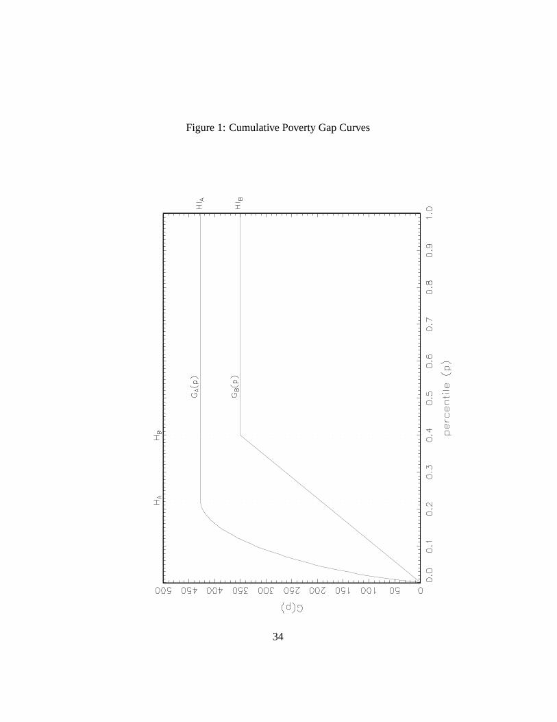
Figure 1: Cumulative Poverty Gap Curves

34

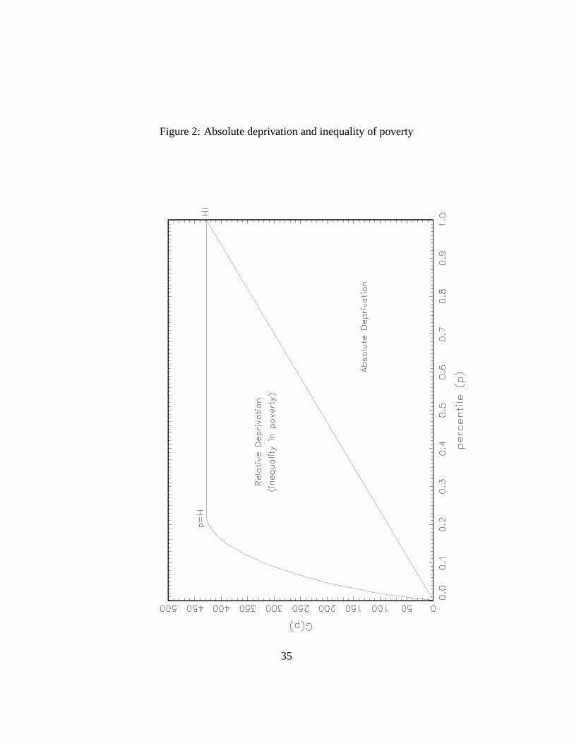
Figure 2: Absolute deprivation and inequality of poverty

35

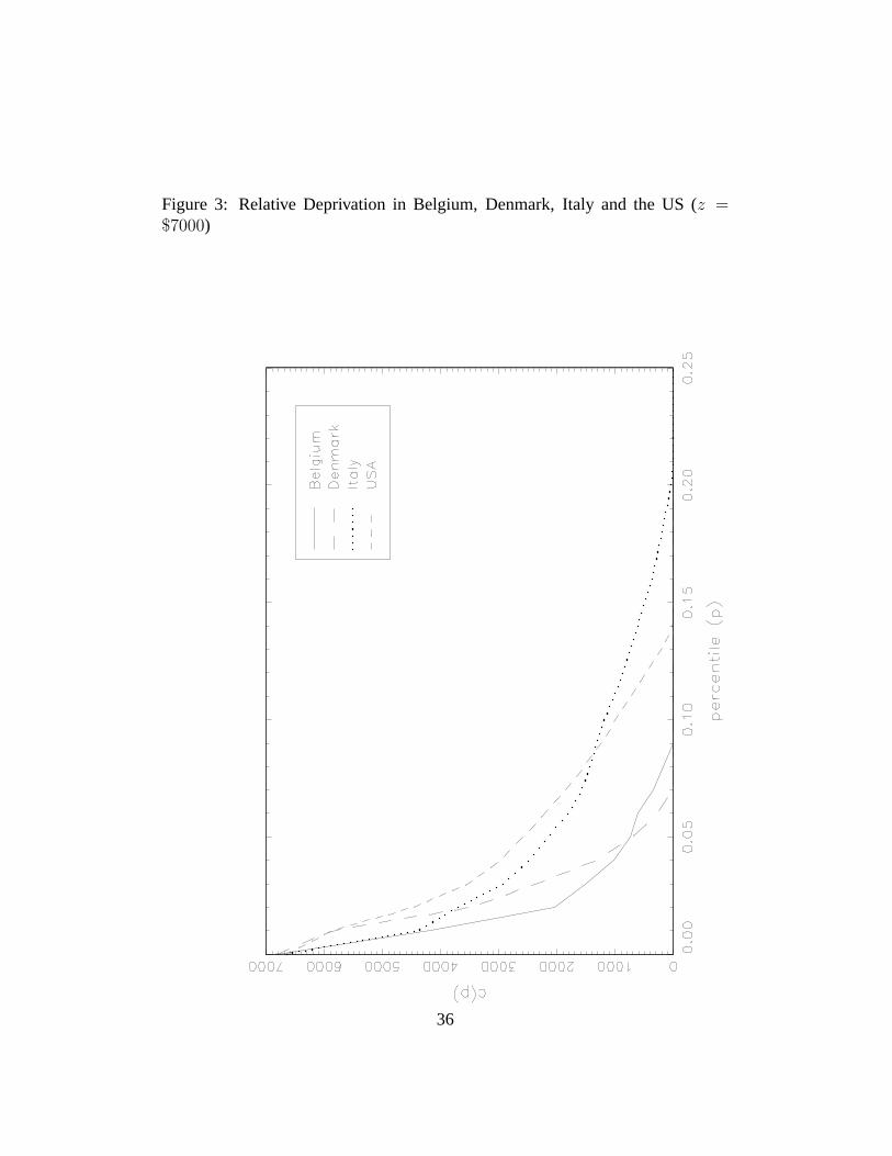
Figure 3: Relative Deprivation in Belgium, Denmark, Italy and the US (z =$7000)

36

Figure 4: CPG curves for Belgium, Denmark, Italy and the US (z=$7000)

37

Figure 5: Difference between the Belgian and the DanishS(v) indices for differentv andz

38

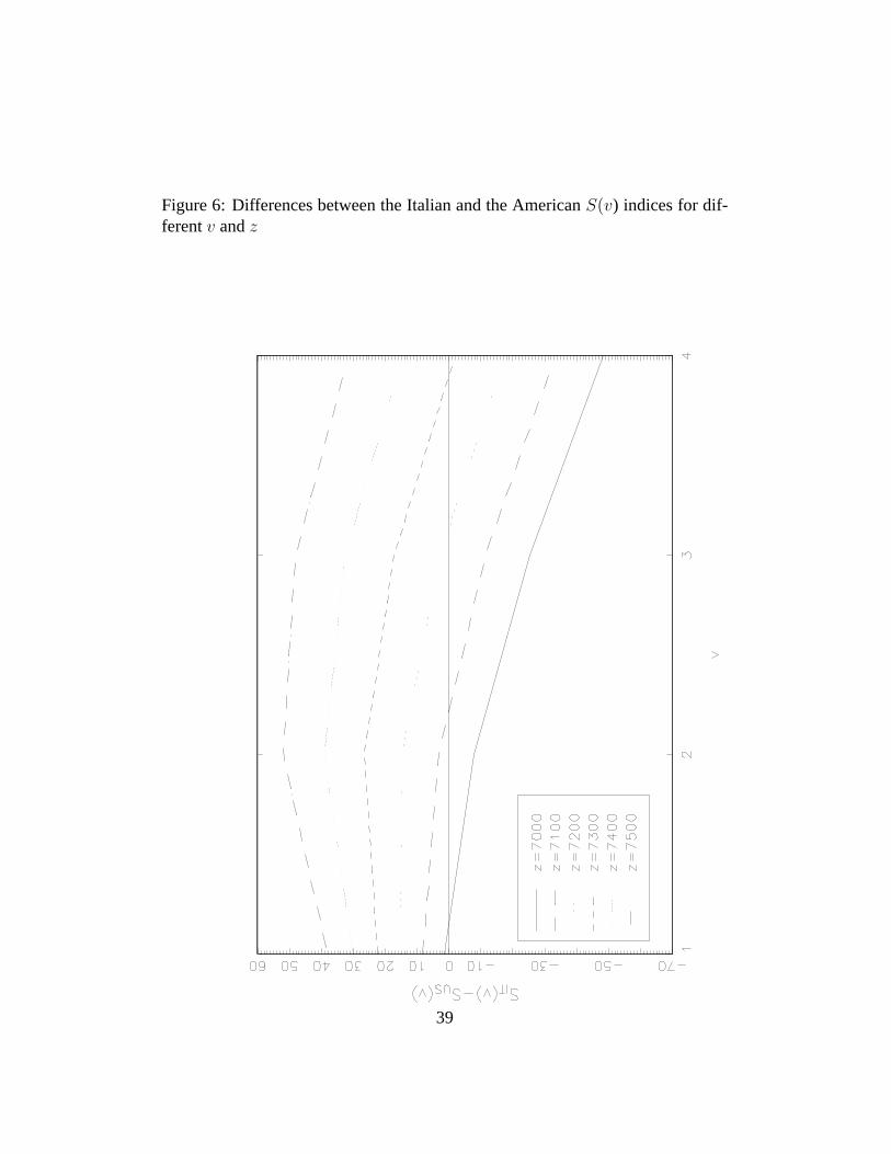
Figure 6: Differences between the Italian and the AmericanS(v) indices for dif-ferentv andz

39

absolute and relative deprivation - lakehead...

Documents