absolute moments of generalized hyperbolic … · absolute moments of generalized hyperbolic...
TRANSCRIPT

Absolute Moments of GeneralizedHyperbolic Distributions and ApproximateScaling of Normal Inverse Gaussian LevyProcesses
OLE EILER BARNDORFF-NIELSEN
Department of Mathematical Sciences, University of Arhus
ROBERT STELZER
Centre for Mathematical Sciences, Munich University of Technology
ABSTRACT. Expressions for (absolute) moments of generalized hyperbolic and normal inverse
Gaussian (NIG) laws are given in terms of moments of the corresponding symmetric laws. For the
(absolute) moments centred at the location parameter l explicit expressions as series containing
Bessel functions are provided. Furthermore, the derivatives of the logarithms of absolute l-centred
moments with respect to the logarithm of time are calculated explicitly for NIG Levy processes.
Computer implementation of the formulae obtained is briefly discussed. Finally, some further
insight into the apparent scaling behaviour of NIG Levy processes is gained.
Key words: generalized inverse Gaussian distribution, normal inverse Gaussian distribution,
scaling
1. Introduction
The generalized hyperbolic (GH) distribution was introduced in Barndorff-Nielsen (1977) in
connection to a study of the grain-size distribution of wind-blown sand. Since then it has been
used in many different areas. Before outlining the contents of the present paper, we now give a
brief overview of various applications of the GH laws and the associated Levy processes.
The original paper by Barndorff-Nielsen (1977) was focused on the special case of the
hyperbolic law. That law and its applicability have been further discussed, inter alia, in
Barndorff-Nielsen et al. (1983, 1985) (particle size distributions of sand), Barndorff-Nielsen &
Christiansen (1988), Hartmann & Bowman (1993), Sutherland & Lee (1994) and references
therein (coastal sediments), Xu et al. (1993) and their list of references (fluid sprays). In
Barndorff-Nielsen (1982) the appearance of the three-dimensional hyperbolic law in relativ-
istic statistical physics was pointed out. Other areas, where hyperbolic distributions have been
employed, include biology (e.g. Blæsild, 1981) and primary magnetization of lava flows (cf.
Kristjansson & McDougall, 1982). Furthermore, in Barndorff-Nielsen et al. (1989) the
hyperbolic distribution is employed to model wind shear data of landing aircrafts parsimo-
niously. See also Barndorff-Nielsen (1979) for applications in turbulence.
Moreover, Barndorff-Nielsen et al. (2004) recently demonstrated (following an indication in
Barndorff-Nielsen, 1998a) that the normal inverse Gaussian (NIG) law, another important
special case of the GH law, is capable of describing velocity data from turbulence experiments
with high accuracy. Eriksson et al. (2004) employ the NIG distribution to approximate other
(unknown) probability distributions.
In recent years many authors have successfully fitted generalized hyperbolic distributions and
in particular NIG laws to returns in financial time series; see Eberlein & Keller (1995), Prause
(1997, 1999), Barndorff-Nielsen (1997), Barndorff-Nielsen & Shephard (2001a,b) and references
� Board of the Foundation of the Scandinavian Journal of Statistics 2005. Published by Blackwell Publishing Ltd, 9600 Garsington
Road, Oxford OX4 2DQ, UK and 350 Main Street, Malden, MA 02148, USA Vol 32: 617–637, 2005

therein, Schoutens (2003), Barndorff-Nielsen & Shephard (2005). Benth & Saltyt _e-Benth (2005)
have recently put forth a model for Norwegian temperature data driven by a GH Levy process.
This has, in particular, led to modelling the time dynamics of financial markets by stochastic
processes using generalized hyperbolic or normal inverse Gaussian laws and associated Levy
processes as building blocks (e.g. Rydberg, 1997, 1999; Bibby & Sørensen, 1997; Barndorff-
Nielsen, 1998b, 2001; Prause, 1999; Raible, 2000; Barndorff-Nielsen & Shephard, 2001a, 2005
and references therein; Eberlein, 2001; Schoutens, 2003; Cont & Tankov, 2004; Rasmus et al.
2004; Emmer & Kluppelberg, 2004; Mencia & Sentana, 2004).
One of the reasons, why the GH distribution is used in such a variety of situations, is that it
is not only flexible enough to fit many different data sets well, but also is rather tractable
analytically, and many important properties (density, characteristic function, cumulant
transform, Levy measure, etc.) are known. Some of these properties are recalled in section 2.
Yet, until now, no details on absolute moments of arbitrary order r > 0 are known, except for
r ¼ 1. Thus we derive, in section 3, formulae for the (absolute) moments of arbitrary order
r > 0 of the generalized hyperbolic distribution in terms of moments of the corresponding
symmetric GH law. For l-centred (absolute) moments, i.e. moments centred at the location
parameter l, we are able to give explicit formulae using Bessel functions. From these general
formulae we will then, as special cases, obtain formulae for the absolute moments of the NIG
law and NIG Levy process. We especially focus on the NIG case because of its wide appli-
cability and tractability. In particular, the NIG Levy process has a marginal NIG distribution
at all times, an appealing feature not shared by the general GH Levy process.
Due to Kolmogorov’s famous laws for homogeneous and isotropic turbulence (see, for
instance, Frisch, 1995) scaling is an important issue when considering turbulence data and
models. Ongoing research indicates that the time transformation carried out in Barndorff-
Nielsen et al. (2004) leads to a process with NIG marginals and very strong apparent scaling.
The question of the possible relevance of scaling in finance was raised by Mandelbrot (1963)
and has since been discussed by a number of authors, see, in particular, Muller et al. (1990),
Guillaume et al. (1997) and Mandelbrot (1997). More recently the question was taken up by
Barndorff-Nielsen&Prause (2001), who showed that anNIGLevy processmay exhibit moment
behaviour which is very close to scaling. However, they solely studied the first absolute moment
and obtained analytic results only in the case of a symmetric NIG Levy process. As part of this
paper we generalize their findings to the skewed case and higher order moments.
Based on the explicit general formulae for l-centred moments of the NIG law, resp. NIG
Levy process, we are able to deduce analytic results for the approximate scaling of an NIG
Levy process, namely explicit expressions for the derivative of the logarithm of the l-centredabsolute moments of the NIG Levy process with respect to the logarithm of time.
In the final sections we discuss the numerical implementation of the formulae obtained and
give numerical examples for the apparent scaling present in NIG Levy processes.
Our results show that, in particular, the occurrence of empirical scaling laws is not bound to
necessitate the use of self-similar or even multifractal processes for modelling, as this type of
behaviour is already exhibited by such simple a model as an NIG Levy process, when looking
at the relevant time horizons. For a survey of the theory and (approximate) occurrence of self-
similarity and scaling, see Embrechts & Maejima (2002).
2. Generalized hyperbolic and inverse Gaussian distributions
In this paper, we consider the class of one-dimensional GH distributions and the subclass
of NIG distributions in particular. The GH law was, as already noted, introduced in Barn-
dorff-Nielsen (1977) and its properties were further studied in Barndorff-Nielsen (1978a),
618 O. E. Barndorff-Nielsen and R. Stelzer Scand J Statist 32
� Board of the Foundation of the Scandinavian Journal of Statistics 2005.

Barndorff-Nielsen & Blæsild (1981) and Blæsild & Jensen (1981). Some recent results, in
particular regarding the multivariate GH laws, can be found in Prause (1999), Eberlein (2001),
Eberlein & Hammerstein (2004) and Mencia & Sentana (2004).
We denote the (one-dimensional) generalized hyperbolic distribution by GH (m, a, b, l, d)and characterize it via its probability density given by:
pðx; m; a; b; l; dÞ ¼ �cm�a1=2�mffiffiffiffiffiffi2p
pdKmð�cÞ
1þ ðx� lÞ2
d2
!m=2�1=4
� Km�1=2 �a
ffiffiffiffiffiffiffiffiffiffiffiffiffiffiffiffiffiffiffiffiffiffiffiffiffi1þ ðx� lÞ2
d2
s0@
1Aebðx�lÞ ð1Þ
for x 2 R and where the parameters satisfy m 2 R, 0 � |b| < a, l 2 R, d 2 R>0, and
c :¼ffiffiffiffiffiffiffiffiffiffiffiffiffiffiffiffiffia2 � b2
q; �a :¼ da; �b :¼ db; �c :¼ dc. Here a can be interpreted as a shape, b as a
skewness, l as a location and d as a scaling parameter; finally, m characterizes subclasses and
primarily influences the tail behaviour.
Furthermore, Km(Æ) denotes the modified Bessel function of the third kind and order m 2 R.
For a comprehensive discussion of Bessel functions of complex arguments see Watson (1952).
Jørgensen (1982) contains an appendix listing important properties of Bessel functions of the
third kind and related functions. Most of these properties can also be found in standard
reference books like Gradshteyn & Ryzhik (1965) or Bronstein et al. (2000). For the following
we need to know that Km is defined on the positive half plane D ¼ fz 2 C : R(z) > 0g of the
complex numbers and is holomorphic on D. From Watson (1952, p. 182) or Jørgensen (1982,
p. 170) we have the representation
KmðzÞ ¼1
2
Z 1
0
ym�1 e�12 zðyþy�1Þ dy; ð2Þ
which shows the strict positivity of Km on R>0. The substitution x :¼ y�1 immediately gives
K�m ¼ Km. Furthermore, Km(z) is obviously monotonically decreasing in z on R>0. From the
alternative representation
KmðzÞ ¼Z 1
0
e�z coshðtÞ coshðmtÞ dt ð3Þ
(cf. Watson, 1952, p. 181) one reads off that, for fixed z 2 R>0, Km(z) is strictly increasing in mfor m 2 R�0.
There are several popular subclasses contained within the GH laws. For m ¼ 1 the hyper-
bolic and for m ¼ �1/2 the normal inverse Gaussian distributions are obtained. The normal,
exponential, Laplace, Variance-Gamma and Student-t distributions are among many others
limiting cases of the GH distribution (cf. Eberlein & Hammerstein, 2004 for a comprehensive
analysis).
Alternatively one often uses
q :¼ ba¼
�b�a; n :¼ ð1þ �cÞ�1=2 and v :¼ qn
to parameterize the GH law, as these quantities are invariant under location-scale changes and
v, resp. n, can be interpreted as a skewness, resp. kurtosis, measure. Moreover, the parameter
restrictions imply 0 < |v| < n < 1. For fixed m this gives rise to the use of shape triangles as a
graphical tool to study generalized hyperbolic distributions (see e.g. Barndorff-Nielsen et al.,
1983, 1985; Barndorff-Nielsen & Christiansen, 1988; Rydberg, 1997; Prause, 1999).
Scand J Statist 32 Absolute moments of GH distributions 619
� Board of the Foundation of the Scandinavian Journal of Statistics 2005.

A very useful representation in law of the generalized hyperbolic distribution can be given
using the generalized inverse Gaussian distribution. The generalized inverse Gaussian distri-
bution GIG(m, d, c) with parameters m 2 R, c, d 2 R�0 and c þ d > 0 is the distribution on
R>0 which has probability density function
pðx; m; d; cÞ ¼ ðc=dÞm
2KmðdcÞxm�1 exp � 1
2ðd2x�1 þ c2xÞ
� �
¼ �cm
2Kmð�cÞd�2mxm�1 exp � 1
2ðd2x�1 þ �c2d�2xÞ
� �: ð4Þ
For more information on the GIG law we refer to Jørgensen (1982) and for an interpretation
in terms of hitting times to Barndorff-Nielsen et al. (1978). The following normal variance–
mean mixture representation of the generalized hyperbolic law holds.
Lemma 1
Let X � GH(m, a, b, l, d), V � GIG(m, d, c) with c ¼ffiffiffiffiffiffiffiffiffiffiffiffiffiffiffia2 � b2
qand e � N(0, 1), where V and
e are independent, then:
X ¼D lþ bV þffiffiffiffiV
pe:
(For a general overview over normal variance–mean mixtures see Barndorff-Nielsen et al.,
1982.)
Furthermore, the cumulant function of the generalized hyperbolic law X �GH(m, a, b, l, d) is given by
Kðh z X Þ ¼ m2log
c
a2 � ðbþ hÞ2
!þ log
Km dffiffiffiffiffiffiffiffiffiffiffiffiffiffiffiffiffiffiffiffiffiffiffiffiffiffiffia2 � ðbþ hÞ2
q� �
Km dffiffiffiffiffiffiffiffiffiffiffiffiffiffiffia2 � b2
q� �0BB@
1CCAþ hl: ð5Þ
Obviously K(h � X) is defined for all h 2 R with |b þ h| < a. From this fact and Barndorff-
Nielsen (1978b, Corollary 7.1) we immediately obtain:
Lemma 2
Assume X � GH(m, a, b, l, d). Then X 2 Lp for all p > 0, i.e. E(|X|p) exists for all p > 0.
One immediately calculates the expected value and variance of a GH-distributed random
variate X to be
EðX Þ ¼ lþ bdKmþ1ð�cÞcKmð�cÞ
;
VarðX Þ ¼ d2Kmþ1ð�cÞ�cKmð�cÞ
þ b2
c2Kmþ2ð�cÞKmð�cÞ
� Kmþ1ð�cÞKmð�cÞ
� �2 ! !
:
Higher order cumulants can also be calculated, but the expressions become more and more
complicated.
In the GH law the existence of moments of all orders is combined with semi-heavy tails
pðx; m; a; b; 0; dÞ � Cjxjm�1 exp ð�aþ bÞxð Þ as x ! �1 ð6Þ
for some constant C.
620 O. E. Barndorff-Nielsen and R. Stelzer Scand J Statist 32
� Board of the Foundation of the Scandinavian Journal of Statistics 2005.

In Fig. 1 the densities of NIG distributions fitted to turbulent velocity increments (from
data set I of Barndorff-Nielsen et al., 2004; with a detailed description of the data) at different
lags are plotted on a logarithmic scale together with histograms of the original data. The
graphs were obtained using the programme �hyp� (Blæsild & Sørensen, 1992). They exemplify
the rich variety of distributional shapes one can already get from the NIG law. Letting m varyoffers the possibility to get even more different shapes (see e.g. Eberlein & Ozkan, 2003 for
some hyperbolic fits). Note especially the marked differences in the centre of the distributions
and the difference in how the asymptote given by (6) is approached. For a lag of 9000 the
shape is already very close to the quadratic one of the Gaussian law.
Moreover, the GH law is infinitely divisible (in fact, self-decomposable) and leads thus to an
associated Levy process. Yet, the GH distribution is not closed under convolution, but the
NIG distribution has this property, so that all marginal distributions of a Levy process
associated with an NIG distribution belong to the NIG class.
The above facts and the analytical tractability due to the existence of explicit expressions for
the density, the cumulant function and related functions makes using the GH law appealing in
many different areas, as already pointed out in the Introduction.
3. Moments and absolute moments of GH laws
In this section, we give expressions for different (absolute) moments of arbitrary GH distri-
butions in terms of moments of corresponding symmetric GH distributions. Based upon this
−3 −2 −1 0 1
−6
−4
−2
log(velocity increments)
log(
dens
ity)
−0.5 0.0 0.5 1.0
−10
−8
−6
−4
−2
0
2
log(velocity increments)
log(
dens
ity)
−2 −1 0 1 2
−8
–10
−6
−4
−2
0
log(velocity increments)
log(
dens
ity)
Fig. 1. Log-density (solid line) of NIG distribution fitted to velocity increments at lags 12 (upper left), 500
(upper right) and 9000 (lower centre) and log-histogram (only top end points are given (�)).
Scand J Statist 32 Absolute moments of GH distributions 621
� Board of the Foundation of the Scandinavian Journal of Statistics 2005.

we obtain explicit expressions for l-centred (absolute) moments of GH distributions,
employing the variance–mean mixture representation.
Theorem 1
Let X � GH(m, a, b, l, d), Y � GH(m, a, 0, l, d), then for every r > 0 and n 2 N:
ðiÞ EðXnÞ ¼ �c�a
� �m Kmð�aÞKmð�cÞ
X1k¼0
bk
k!EðY nðY � lÞkÞ
ðiiÞ EðjX jrÞ ¼ �c�a
� �m Kmð�aÞKmð�cÞ
X1k¼0
bk
k!EðjY jrðY � lÞkÞ
ðiiiÞ EððX � lÞnÞ ¼ �c�a
� �m Kmð�aÞKmð�cÞ
X1k¼0
b2kþm
ð2k þ mÞ!EððY � lÞ2kþmþnÞ
ðivÞ EðjX � ljrÞ ¼ �c�a
� �m Kmð�aÞKmð�cÞ
X1k¼0
b2k
ð2kÞ!EðjY � lj2kþrÞ;
where m :¼ n mod 2. All moments above are finite.
Note that from the cumulant function we have E(Y) ¼ l and EðX Þ ¼ lþbdKmþ1ð�cÞ=ðcKmð�cÞÞ, as stated before. Hence, we have that E((Y � l)r) are central moments,
whereas E((X � l)r) are in general just l-centred moments. Note also that sgn E((X � l)n ¼sgn b for all odd n.
Proof. We will only prove (ii), as the proofs of the other formulae proceed along the same
lines, except that to obtain (iii) and (iv) one notes in the final step that odd central moments of
Y vanish, as the distribution of Y is symmetric around l.The series representation of the exponential function gives
EðjX jrÞ ¼ZR
�cm�a1=2�mffiffiffiffiffiffi2p
pdKmð�cÞ
1þ ðx� lÞ2
d2
!m=2�1=4
� Km�1=2 �a
ffiffiffiffiffiffiffiffiffiffiffiffiffiffiffiffiffiffiffiffiffiffiffiffiffi1þ ðx� lÞ2
d2
s0@
1Aebðx�lÞjxjr dx
¼ZR
X1k¼0
�cm�a1=2�mffiffiffiffiffiffi2p
pdKmð�cÞ
1þ ðx� lÞ2
d2
!m=2�1=4
� Km�1=2 �a
ffiffiffiffiffiffiffiffiffiffiffiffiffiffiffiffiffiffiffiffiffiffiffiffiffi1þ ðx� lÞ2
d2
s0@
1A bk
k!ðx� lÞk jxjr dx:
The integrals exist (cf. lemma 2) and the same is true with b changed to �b. This implies that
the integrals
Z 1
l
�cm�a1=2�mffiffiffiffiffiffi2p
pdKmð�cÞ
1þ ðx� lÞ2
d2
!m=2�1=4
Km�1=2 �a
ffiffiffiffiffiffiffiffiffiffiffiffiffiffiffiffiffiffiffiffiffiffiffiffiffi1þ ðx� lÞ2
d2
s0@
1Aejbðx�lÞjjxjr dx
and
Z l
�1
�cm�a1=2�mffiffiffiffiffiffi2p
pdKmð�cÞ
1þ ðx� lÞ2
d2
!m=2�1=4
Km�1=2 �a
ffiffiffiffiffiffiffiffiffiffiffiffiffiffiffiffiffiffiffiffiffiffiffiffiffi1þ ðx� lÞ2
d2
s0@
1Aejbðx�lÞjjxjr dx
and hence the integral
622 O. E. Barndorff-Nielsen and R. Stelzer Scand J Statist 32
� Board of the Foundation of the Scandinavian Journal of Statistics 2005.

ZR
�cm�a1=2�mffiffiffiffiffiffi2p
pdKmð�cÞ
1þ ðx� lÞ2
d2
!m=2�1=4
Km�1=2 �a
ffiffiffiffiffiffiffiffiffiffiffiffiffiffiffiffiffiffiffiffiffiffiffiffiffi1þ ðx� lÞ2
d2
s0@
1Aejbðx�lÞjjxjr dx
exist. Using the last one as majorant, Lebesgue’s convergence theorem gives
EðjX jrÞ ¼X1k¼0
ZR
�cm�a1=2�mffiffiffiffiffiffi2p
pdKmð�cÞ
1þ ðx� lÞ2
d2
!m=2�1=4
� Km�1=2 �a
ffiffiffiffiffiffiffiffiffiffiffiffiffiffiffiffiffiffiffiffiffiffiffiffiffi1þ ðx� lÞ2
d2
s0@
1A bk
k!ðx� lÞk jxjr dx
¼X1k¼0
bk
k!�c�a
� �m Kmð�aÞKmð�cÞ
ZR
�am�a1=2�mffiffiffiffiffiffi2p
pdKmð�aÞ
1þ ðx� lÞ2
d2
!m=2�1=4
� Km�1=2 �a
ffiffiffiffiffiffiffiffiffiffiffiffiffiffiffiffiffiffiffiffiffiffiffiffiffi1þ ðx� lÞ2
d2
s0@
1Aðx� lÞk jxjr dx:
From this we immediately conclude
EðjX jrÞ ¼ �c�a
� �m Kmð�aÞKmð�cÞ
X1k¼0
bk
k!E jY jrðY � lÞk� �
:
Corollary 1
Let X � GH(m, a, b, l, d), V � GIG(m, d, a) and e � N(0, 1) with V and e independent, then
for every r > 0 and n 2 N:
ðiÞ EððX � lÞnÞ ¼ �c�a
� �m Kmð�aÞKmð�cÞ
X1k¼0
b2kþm
ð2k þ mÞ!E V kþðmþnÞ=2� �
E �2kþmþn� �
ðiiÞ EðjX � ljrÞ ¼ �c�a
� �m Kmð�aÞKmð�cÞ
X1k¼0
b2k
ð2kÞ!E V kþr=2� �
E j�j2kþr� �
;
where m :¼ n mod 2.
Proof. Combine theorem 1 with lemma 1.
Note that we obtain the (absolute) moments of X provided l ¼ 0 and the (absolute) central
moments if b ¼ 0. For b ¼ 0 the above series are in fact just a single term or vanish com-
pletely.
Using the explicit expressions for the moments of GIG and normal laws, given in appendix
A, it is now straightforward to obtain more explicit expressions for the l-centred (absolute)
moments of GH laws.
Theorem 2
Let X � GH(m, a, b, l, d), then for every r > 0 and n 2 N:
ðiÞ EððX � lÞnÞ ¼ 2n2d e�cmd2 n
2d ebmffiffiffip
pKmð�cÞ�amþ
n2d eX1k¼0
2k�b2kC k þ n2
� þ 1
2
� ��akð2k þ mÞ! Kmþkþ n
2d eð�aÞ
ðiiÞ EðjX � ljrÞ ¼ 2r2�cmdrffiffiffi
pp
Kmð�cÞ�amþr2
X1k¼0
2k�b2kC k þ r2 þ 1
2
� ��akð2kÞ! Kmþkþr
2ð�aÞ;
where m :¼ n mod 2.
Scand J Statist 32 Absolute moments of GH distributions 623
� Board of the Foundation of the Scandinavian Journal of Statistics 2005.

Proof. Combine corollary 1 with lemmas 4 and 5 noting that (n þ m) mod 2 ¼ 0 and
(m þ n)/2 ¼ (n mod 2 þ n)/2 ¼ dn/2e.The absolute convergence of the series on the right-hand sides is obviously implied by the
finiteness of E((X � l)n), resp. E(|X � l|r), and the positivity of all terms involved. Yet, one
can also immediately give an analytic argument, which adds further insight into the conver-
gence behaviour and is useful when one implements the above formulae on a computer (see
section 6). Let
ak :¼2k�b2kC k þ r
2 þ 12
� ��akð2kÞ! Kmþkþr
2ð�aÞ:
From KmðzÞ �ffiffiffiffiffiffiffiffiffiffiffiffiðp=2Þ
p2mmm�1=2 e�mz�m for m ! 1 (Ismail, 1977; Jørgensen, 1982, p. 171) we
obtain
akþ1
ak�
4�b2 k þ r2 þ 1
2
� �k þ mþ r
2
� �1þ 1
kþmþr2
� �kþmþrþ12
�a2eð2k þ 2Þð2k þ 1Þ !k!1 �b�a
� �2
< 1 ð7Þ
and thus the quotient criterion from standard analysis implies absolute convergence. Lemma
6, which we give in appendix B2, and its proof add some further insight into the behaviour of
the series.
As a side result of theorem 2 we also obtain two identities for modified Bessel functions of
the third kind.
Corollary 2
Let x, y, z 2 R>0 s.t. z ¼ffiffiffiffiffiffiffiffiffiffiffiffiffiffiffix2 � y2
pand m 2 R then
ðiÞ KmðzÞ ¼zm
xmX1k¼0
1
2k � k!y2k
xkKmþkðxÞ
ðiiÞ zKmðzÞ þ y2Kmþ1ðzÞ ¼zmþ1
xmX1k¼0
2k þ 1
2k � k!y2k
xkKmþkðxÞ:
Proof. Combine theorem 2 with
EðX Þ ¼ d�b�cKmþ1ð�cÞKmð�cÞ
and EðX 2Þ ¼ d2Kmþ1ð�cÞ�cKmð�cÞ
þ�b2
�c2Kmþ2ð�cÞKmð�cÞ
� �
for X � GH(m, a, b, 0, d) and use Cðn þ 1=2Þ ¼ ð2nÞ!ffiffiffip
p=ð22n � n!Þ. Finally identify x, y, z, m
with �a; �b; �c; m þ 1.
4. Moments of NIG laws
We now turn to the normal inverse Gaussian subclass of the generalized hyperbolic law. For
an overview see especially Barndorff-Nielsen (1998b). Recall that the NIG(a, b, l, d) law with
0 � |b| < a, l 2 R and d 2 R>0 is the special case of the GH(m, a, b, l, d) law given by m ¼� 1/2, as already mentioned when summarizing the properties of the GH law previously.
Hence, our above calculations for (l-centred) moments immediately lead to the following.
Corollary 3
Let X � NIG(a, b, l, d), Y � NIG(a, 0, l, d), then for every r > 0 and n 2 N:
624 O. E. Barndorff-Nielsen and R. Stelzer Scand J Statist 32
� Board of the Foundation of the Scandinavian Journal of Statistics 2005.

ðiÞ EðXnÞ ¼ e�c��aX1k¼0
bk
k!EðY nðY � lÞkÞ
ðiiÞ EðjX jrÞ ¼ e�c��aX1k¼0
bk
k!EðjY jrðY � lÞkÞ
ðiiiÞ EððX � lÞnÞ ¼ 2n2d eþ1
2d2n2d ebm
p�an2d e�1
2
e�cX1k¼0
2k�b2kC k þ n2
� þ 1
2
� ��akð2k þ mÞ! Kkþ n
2d e�12ð�aÞ
ðivÞ EðjX � ljrÞ ¼ 2rþ12 dr
p�ar�12
e�cX1k¼0
2k�b2kC k þ rþ12
� ��akð2kÞ! Kkþr�1
2ð�aÞ;
where m :¼ n mod 2. All moments above are finite.
Proof. Follows immediately from theorems 1 and 2 using K1=2ðzÞ ¼ K�1=2ðzÞ ¼ffiffiffiffiffiffiffiffiffiffiffiffiðp=2Þ
pz�1=2 e�z (see e.g. Jørgensen, 1982, p. 170).
Formulae (iii) and (iv) for r equal to an even natural number can be given more explicitly
using
Knþ12ðzÞ ¼ K1
2ðzÞ 1þ
Xni¼1
ðnþ iÞ!i!ðn� iÞ! 2
�iz�i
!ð8Þ
for all n 2 N (see e.g. Jørgensen, 1982, p. 170). But in order to avoid making the above
formulae even more complex, we omit this.
5. Moments of NIG Levy processes and their time-wise behaviour
Based on the above results our aim now is to generalize the findings of Barndorff-Nielsen &
Prause (2001) regarding the time-wise approximate scaling behaviour of NIG Levy processes.
5.1. Moments of NIG Levy processes
Let Z(t), t 2 R>0, be the NIG(a, b, l, d) Levy process, i.e. the Levy process for which
Z(1) � NIG(a, b, l, d). Owing to the closedness under convolution of the NIG law, the
marginal distribution of the NIG Levy process at an arbitrary time t 2 R>0 is given by
NIG(a, b, tl, td). For more background on NIG Levy processes see in particular Barn-
dorff-Nielsen (1998b). From our previous results we can immediately infer the following:
Corollary 4
Let Z(t), t 2 R>0, be an NIG(a, b, l, d) Levy process, then for every r > 0 and n 2 N:
ðiÞ EððZðtÞ � ltÞnÞ ¼ 2n2d eþ1
2d2n2d ebm
p�an2d e�1
2
et�cX1k¼0
2k�b2kC k þ n2
� þ 1
2
� ��akð2k þ mÞ! tkþ
n2d eþ1
2
� Kkþ n2d e�1
2ðt�aÞ
ðiiÞ EðjZðtÞ � ltjrÞ ¼ 2rþ12 dr
p�ar�12
et�cX1k¼0
2k�b2kC k þ rþ12
� ��akð2kÞ! tkþðrþ1Þ=2Kkþr�1
2ðt�aÞ
where m :¼ n mod 2.
In appendix B2 it is shown that the moments above are analytic functions of time (lemma 6).
This fact is later needed to calculate derivatives of log moments.
Scand J Statist 32 Absolute moments of GH distributions 625
� Board of the Foundation of the Scandinavian Journal of Statistics 2005.

5.2. Scaling and apparent scaling
Before we now turn to discussing the scaling properties of an NIG Levy process, let us
briefly state what scaling precisely means. Let X(t) be some stochastic process. We say
some moment of X obeys a scaling law, if the logarithm of this moment is an affine
function of log time, i.e. for the rth absolute moment, ln E(|X(t)|r) ¼ sr ln t þ cr for some
constants sr, cr 2 R. Here sr is called the scaling coefficient. If all (absolute) moments of X,
or at least those one is interested in, follow a scaling law, we say that the process itself
obeys one. For example, in the case of Brownian motion X(t) with drift l we know from
X ðtÞ � lt¼Dffiffit
pðX ð1Þ � lÞ that ln E(|X(t) � lt|r) ¼ (r/2) ln t þ constant for all r > 0, i.e.
all absolute moments exhibit scaling. More generally all self-similar processes, e.g. the
strictly a-stable Levy processes (cf. Samorodnitsky & Taqqu, 1994, Chapter 7; Sato, 1999,
Chapter 3), obey a scaling law. When looking only at small changes in time the local
scaling behaviour is determined by d ln E(|X(t)|r)/d ln t (in the case of the rth absolute
moment). In the presence of scaling the latter derivative is constant and equals the value of
the scaling coefficient. Provided some log moment of a process X(t) exhibits a very close to
affine dependence on log time over some time horizon of interest, we speak of approximate
or apparent scaling. This is equivalent to the local scaling varying only little over the time
spans considered. When working with real empirical data, it is often not possible to
distinguish between apparent and strict scaling due to the randomness of the available
observations. Hence, it is of interest, from a statistical point of view, whether some given
theoretical process shows approximate scaling.
5.3. The time-wise behaviour of l-centred moments
Let us now examine the scaling behaviour exhibited by the NIG(a, b, l, d) Levy process Z(t).
For the following discussion of the time dependence of E(|Z(t) � lt|r) we will abbreviate the
time-independent terms:
cðrÞ :¼ 2rþ12 dr
p�ar�12
ð9Þ
akðrÞ :¼2k�b2kC k þ rþ1
2
� ��akð2kÞ! : ð10Þ
If we define
wðtÞ :¼ expðt�cÞX1k¼0
akðrÞtkþðrþ1Þ=2Kkþðr�1Þ=2ðt�aÞ ð11Þ
and
/ðtÞ :¼ lnwðetÞ; ð12Þ
we have from corollary 4 that
EðjZðtÞ � ltjrÞ ¼ cðrÞ � wðtÞ ð13Þ
and
lnEðjZðtÞ � ltjrÞ ¼ ln cðrÞ þ /ðln tÞ: ð14Þ
626 O. E. Barndorff-Nielsen and R. Stelzer Scand J Statist 32
� Board of the Foundation of the Scandinavian Journal of Statistics 2005.

Thus:
d lnEðjZðtÞ � ltjrÞd ln t
¼ /0ðln tÞ: ð15Þ
Lemma 3
Let / : R>0 ! R be defined by (12), then
/0ðtÞ ¼ 1þ �c et � �a et
P1k¼0
akðrÞ etkKkþðr�3Þ=2ðet�aÞ
P1k¼0
akðrÞ etkKkþðr�1Þ=2ðet�aÞ: ð16Þ
Proof. Using
K 0mðzÞ ¼ �Km�1ðzÞ � mz�1KmðzÞ ð17Þ
(see e.g. Jørgensen, 1982, p. 170 or Bronstein et al., 2000, p. 528), we obtain for w(t) as definedin equation (11):
w0ðtÞ ¼ expðt�cÞ �cX1k¼0
akðrÞtkþðrþ1Þ=2Kkþðr�1Þ=2ðt�aÞ þX1k¼0
akðrÞ k þ r þ 1
2
� �
� tkþðr�1Þ=2Kkþðr�1Þ=2ðt�aÞ �X1k¼0
akðrÞtkþðrþ1Þ=2�a
� Kkþðr�3Þ=2ðt�aÞ þ k þ r � 1
2
� �ðt�aÞ�1Kkþr�1
2ðt�aÞ
� ��
¼ �cwðtÞ þ t�1wðtÞ � �a e�ctX1k¼0
akðrÞtkþðrþ1Þ=2Kkþðr�3Þ=2ðt�aÞ:
That we may interchange differentiation and summation above is an immediate consequence
of lemma 6 and Weierstra�s theorem for sequences of holomorphic functions (see appendix
B1). Hence, we get from (12)
/0ðtÞ ¼ etw0ðetÞwðetÞ ¼ 1þ �c et � �a et
P1k¼0
akðrÞ etðkþðrþ1Þ=2ÞKkþðr�3Þ=2ðet�aÞ
P1k¼0
akðrÞ etðkþðrþ1Þ=2ÞKkþðr�1Þ=2ðet�aÞ:
Now we can formulate our main result on the scaling behaviour of NIG Levy processes.
Theorem 3
Let Z(t), t 2 R>0, be an NIG(a, b, l, d) Levy process, then
d lnEðjZðtÞ � ltjrÞd ln t
¼ 1þ �ct � �at
P1k¼0 akðrÞtkKkþðr�3Þ=2ð�atÞP1k¼0 akðrÞtkKkþðr�1Þ=2ð�atÞ
for every r > 0.
Proof. The result follows by combining lemma 3 and (15).
When comparing the above results with Barndorff-Nielsen & Prause (2001) note that they
looked at the derivatives with respect to lnð�atÞ, whereas we look at the derivative with respect
Scand J Statist 32 Absolute moments of GH distributions 627
� Board of the Foundation of the Scandinavian Journal of Statistics 2005.

to ln t. The difference is related to the fact that Barndorff-Nielsen & Prause (2001) only
consider the case b ¼ 0. In the general case the parameters �a and �b of the marginals at time t
are both scaled with t. Hence, it is most natural and convenient to consider the change of the
log moments versus the change of log time directly.
The expression for the local scaling behaviour derived in theorem 3 is in general not con-
stant in time, hence, the absolute l-centred moments of an NIG Levy process do not obey a
strict scaling law. Later we shall see from numerical examples that apparent scaling is com-
mon. If we look at the symmetric NIG Levy process, i.e. b ¼ 0, the above formula becomes
d lnEðjZðtÞ � ltjrÞd ln t
¼ 1þ �at � �atKðr�3Þ=2ð�atÞKðr�1Þ=2ð�atÞ
: ð18Þ
From this one deducts using Km ¼ K�m that the second l-centred moment obeys a scaling law
with slope 1, which is the same as for Brownian motion.
The aggregational Gaussianity of NIG Levy processes (due to the central limit theorem the
marginal distribution at time t of any Levy process with finite second moment gets more and
more Gaussian as t increases) becomes visible in the asymptotic scaling of the symmetric case
for large times. For r ¼ 1 it was already noted in Barndorff-Nielsen & Prause (2001) that the
local scaling approaches 1/2 for t ! 1 and hence for large t the first absolute l-centredmoment of the process seems to scale like Brownian motion. Using formula (ii) in corollary 4,
which for b ¼ 0 becomes
EðjZðtÞ � ltjrÞ ¼ 2rþ12 dr
p�ar�12
exp t�að ÞC r þ 1
2
� �tðrþ1Þ=2Kr�1
2ðt�aÞ; ð19Þ
and KmðxÞ �ffiffiffiffiffiffiffiffiffiffiffiffiðp=2Þ
px�1=2 e�x for x ! 1 (cf. Jørgensen, 1982, p. 171 or Bronstein et al., 2000)
we get that ln E(|Z(t) � lt|r) � (r/2) ln t þ c for t ! 1, where c 2 R is a constant. Note
that, as usual, ‘�� denotes asymptotic equivalence. Hence, E(|Z(t) � lt|r) obeys a scaling law
with slope r/2 for t ! 1, i.e. the symmetric NIG Levy process approaches the exact scaling
behaviour of Brownian motion. This result can also be easily deduced from (18) using an
asymptotic expansion of K(r�3)/2(z)/K(r�1)/2(z) for z ! þ 1 (see e.g. Jørgensen, 1982, p. 173).
Studying the limiting behaviour of the absolute l-centred moments analytically for b 6¼ 0
seems hardly possible. Yet, numerical studies indicate that a skewed NIG Levy process does
not scale like Brownian motion for large times in general. For example, when computing
d ln E((Z(t))2)/d ln t of the NIG(100, 30, 0, 0.001) Levy process for times from 1/2 to 1024 the
values increase monotonically from 1.004 to 6.268. If we are, however, close to the symmetric
case, i.e. if |b|/a is small, then basically the same approximate scaling behaviour is obtained as
in the symmetric case. This can, in particular, be seen in the numerical data presented in
section 7, where for large times the value of d ln E(|Z(t) � lt|r)/d ln t is very close to the
Brownian motion scaling slope of r/2.
To see from (19) what happens in the symmetric case for t ! 0 we employ the fact that
KmðxÞ � CðmÞ2m�1x�m for m > 0; x & 0� ln x for m ¼ 0; x & 0
ð20Þ
(see e.g. Jørgensen, 1982, p. 171). For r ¼ 1 and t ! 0 we obtain that ln E(|Z(t) � lt|)becomes ln t þ �a eln t þ lnð� lnðt�aÞÞ þ c with c 2 R being a constant. From this we conclude
that for small values of t the first absolute l-centred moment approximately scales with slope
1, as already noted in Barndorff-Nielsen & Prause (2001). The same asymptotic scaling slope
of one holds for r > 1, since lnEðjZðtÞ � ltjrÞ � ln t þ �a eln t þ cðrÞ for t ! 0. Yet, a
628 O. E. Barndorff-Nielsen and R. Stelzer Scand J Statist 32
� Board of the Foundation of the Scandinavian Journal of Statistics 2005.

different result is obtained for 0 < r < 1. In this case one obtains again using (20) and the
identity K�m ¼ Km that lnEðjZðtÞ � ltjrÞ � r ln t þ �a eln t þ cðrÞ and so there is asymptotic
scaling with slope r.
6. Notes on the numerical implementation
We will now briefly discuss some issues related to the implementation of formula (ii) in
corollary 4 and theorem 3 on a computer. Similar results hold for formula (i) of corollary 4.
First note that (ii) in corollary 4 can be reexpressed using (10) as:
EðjZðtÞ � ltjrÞ ¼ 2d2t�a
� �r=2 ffiffiffiffiffiffiffi2t�a
p
pexp t�cð Þ
X1k¼0
akðrÞtkKkþr�12ðt�aÞ: ð21Þ
The value of the infinite series can only be approximated. Yet, note that the analytic con-
vergence discussion of the series in section 3, especially formula (7), implies asymptotically
geometric convergence of this series, which is the faster, the smaller |b| is relatively to a. We
suggest to compute the individual summands recursively as discussed below, add them up and
stop, when summands become negligible compared to the current value of the approximation.
To calculate the individual summands recursively note that
a0ðrÞ ¼ Cr þ 1
2
� �ð22Þ
and
akðrÞtk ¼2�b2ðk þ ðr � 1Þ=2Þ
�að2k � 1Þð2kÞ t � ak�1ðrÞtk�1; ð23Þ
which is obtained using the functional equation C(z þ 1) ¼ zC(z) of the Gamma function, and
that the recursion formula for Bessel functions (Jørgensen, 1982, p. 170) gives
Kkþr�12ðt�aÞ ¼ 2 � k � 1þ r � 1
2
� �ðt�aÞ�1Kk�1þr�1
2ðt�aÞ þ Kk�2þr�1
2ðt�aÞ: ð24Þ
The latter formula implies that we can calculate the values of the Bessel functions needed from
a two-term recursion, for which we only need to calculate K�1þðr�1Þ=2ðt�aÞ and Kðr�1Þ=2ðt�aÞ asstarting values. Hence, the calculation of the value of the series involves, apart from basic
manipulations, only one evaluation of the Gamma function and two of the Bessel functions.
The series in the denominator in theorem 3 is the series just discussed above and the
numerator is of the same type, only the index of the Bessel functions is changed, and can hence
be calculated analogously. Actually, both series can be calculated simultaneously using only
the recursion for ak(r)tk and the two-term recursion for the Bessel functions described above.
There is, however, one possible problem when using the two-term recursion. If the starting
values are zeros up to numerical precision, then only zeros will be calculated as summands. For
example when using Matlab and the built in function for Km one gets K0(z) ¼ 0 for z > 697.
Hence, one needs to take care of this possible case. Provided the recursion works, the numerical
results obtained are usually almost identical to the numerical results one getswhenusing a built in
Bessel function routine of e.g.Matlab for each summand, but the recursionmay save computing
power. Furthermore, it should now be obvious, how numerical evaluations of the formulae for
l-centred (absolute) moments of GH laws given in theorem 2 can be organized efficiently.
The Matlab code we used to produce the numerical results in this paper is available from
http://www.ma.tum.de/stat/Papers. It is based upon the above considerations and can be used
Scand J Statist 32 Absolute moments of GH distributions 629
� Board of the Foundation of the Scandinavian Journal of Statistics 2005.

to compute l-centred moments of the NIG distribution/Levy process and the derivatives of
the log moments with respect to log time.
7. Apparent scaling behaviour of NIG Levy processes
The aim of this section is to show that NIG Levy processes may well exhibit a behaviour very
close to strict scaling over a wide range of orders of moments. We exemplify the possible
apparent scaling of absolute l-centred moments of NIG Levy processes using the parameters
from Barndorff-Nielsen & Prause (2001). They considered the USD/DEM exchange rate from
the whole of 1996, contained in the HFDF96 data set from Olsen & Associates, and fitted an
NIG Levy process to the log returns by maximum likelihood estimation. The estimates
obtained based on the 3-hr log returns are a ¼ 415.9049, b ¼ 1.512, d ¼ 0.0011 and l ¼0.000026. For further details on the data, the estimation procedure and the relevance for
finance we refer the interested reader to the paper by Barndorff-Nielsen & Prause. Note
especially that, as is typical for returns of exchange rate series, l is very close to zero and
therefore there is practically no difference between moments and l-centred moments. Figure 2
(left), which depicts the logarithm of the first absolute l-centred moment versus the logarithm
of time in seconds, is therefore optically indistinguishable from the figure in Barndorff-Nielsen
& Prause (2001) showing the first absolute moment calculated via numerical integration. The
estimated regression line of the log moments against log time, fitted by least squares, has slope
0.5863, which is slightly higher than the slope 0.5705 reported in Barndorff-Nielsen & Prause
(2001), and d ln E(|Z(t) � lt|)/d ln t decreases from 0.7853 to 0.5011 over the time interval
depicted, which is 5.625 min to 32 days. This is significantly different from the Brownian
motion case, where it is exactly 1/2 (cf. above). The behaviour of d ln E(|Z(t) � lt|)/d ln t
over the time interval considered indicates that for t ! 1 the slope asymptotically becomes
about 1/2, the exact Gaussian scaling coefficient. This is related to the fact that |b| is relativelysmall, as already pointed out earlier in the discussion of the scaling asymptotics.
With our results obtained above it is possible to study the behaviour of moments other than
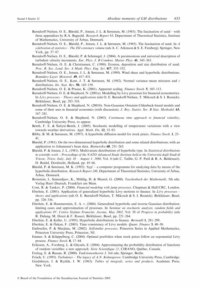
the first. Figures 2 (right), 3 (left, right) and 4 (left) show the time behaviour of the 0.9th, 1.1th,
0.5th and 1.5th l-centred absolute moments over the same time horizon. All figures exhibit
apparent scaling, which improves with the order of the moment. The fitted regression lines
have slope 0.53535, 0.63536, 0.31322 and 0.81327, respectively, which are all higher than the
5 6 7 8 9 10 11 12 13 14 15−10
−9
−8
−7
−6
−5
−4
−3
ln(t) in seconds
ln (
E|Z
(t) −
tm|1
.0)
ln (
E|Z
(t) −
tm|0
.9)
5 6 7 8 9 10 11 12 13 14 15−9
−8
−7
−6
−5
−4
−3
ln(t) in seconds
Fig. 2. Approximate scaling law for the first (left) and 0.9th l-centred absolute moment of the NIG Levy
process fitted to the USD/DEM exchange rate: moments (d) and regression line log moments against log
time.
630 O. E. Barndorff-Nielsen and R. Stelzer Scand J Statist 32
� Board of the Foundation of the Scandinavian Journal of Statistics 2005.
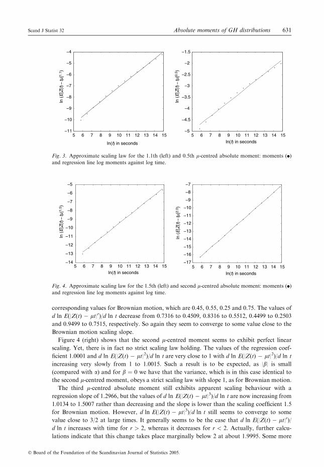
corresponding values for Brownian motion, which are 0.45, 0.55, 0.25 and 0.75. The values of
d ln E(|Z(t) � lt|r)/d ln t decrease from 0.7316 to 0.4509, 0.8316 to 0.5512, 0.4499 to 0.2503
and 0.9499 to 0.7515, respectively. So again they seem to converge to some value close to the
Brownian motion scaling slope.
Figure 4 (right) shows that the second l-centred moment seems to exhibit perfect linear
scaling. Yet, there is in fact no strict scaling law holding. The values of the regression coef-
ficient 1.0001 and d ln E(|Z(t) � lt|2)/d ln t are very close to 1 with d ln E(|Z(t) � lt|2)/d ln t
increasing very slowly from 1 to 1.0015. Such a result is to be expected, as |b| is small
(compared with a) and for b ¼ 0 we have that the variance, which is in this case identical to
the second l-centred moment, obeys a strict scaling law with slope 1, as for Brownian motion.
The third l-centred absolute moment still exhibits apparent scaling behaviour with a
regression slope of 1.2966, but the values of d ln E(|Z(t) � lt|3)/d ln t are now increasing from
1.0134 to 1.5007 rather than decreasing and the slope is lower than the scaling coefficient 1.5
for Brownian motion. However, d ln E(|Z(t) � lt|3)/d ln t still seems to converge to some
value close to 3/2 at large times. It generally seems to be the case that d ln E(|Z(t) � lt|r)/d ln t increases with time for r > 2, whereas it decreases for r < 2. Actually, further calcu-
lations indicate that this change takes place marginally below 2 at about 1.9995. Some more
5 6 7 8 9 10 11 12 13 14 15−14
−13
−12
−11
−10
−9
−8
−7
−6
−5
ln(t) in seconds
ln (
E|Z
(t) −
tm|1
.5)
ln (
E|Z
(t) −
tm|2
.0)
5 6 7 8 9 10 11 12 13 14 15−17
−16
−15
−14
−13
−12
−11
−10
−9
−8
−7
ln(t) in seconds
Fig. 4. Approximate scaling law for the 1.5th (left) and second l-centred absolute moment: moments (d)
and regression line log moments against log time.
5 6 7 8 9 10 11 12 13 14 15−11
−10
−9
−8
−7
−6
−5
−4
ln(t) in seconds
ln (
E|Z
(t) −
tm|1
.1)
ln (
E|Z
(t) −
tm|0
.5)
5 6 7 8 9 10 11 12 13 14 15−5
−4.5
−4
−3.5
−3
−2.5
−2
−1.5
ln(t) in seconds
Fig. 3. Approximate scaling law for the 1.1th (left) and 0.5th l-centred absolute moment: moments (d)
and regression line log moments against log time.
Scand J Statist 32 Absolute moments of GH distributions 631
� Board of the Foundation of the Scandinavian Journal of Statistics 2005.

numerical calculations hint that in the symmetric case ln E(|Z(t) � lt|r) is concave as a
function of ln t for 0 < r � 2 and convex for r � 2.
For very high values of r, i.e. 10 and greater, no apparent linear scaling is observed over the
time horizon considered. Looking at the slopes of the apparent scaling of the l-centredabsolute moments (of orders 0.2–4, for instance, as we have done in further calculations), the
relationship between scaling coefficient and order is apparently not simply linear as, for
example, in the case of an a-stable Levy process (see Samorodnitsky & Taqqu, 1994, Chapter
7; Sato, 1999, Chapter 3), but a concave one.
Our results obtained above show that NIG Levy processes may exhibit something close to
scaling. These findings are particularly interesting, as both in finance, especially when dealing
with foreign exchange returns, and turbulence there is on the one hand empirical and for
turbulence also theoretical evidence of scaling laws, and on the other hand models based on
NIG Levy processes have been put forth in the literature. Compared to Brownian motion the
NIG Levy process does in general not exhibit exact linear scaling, but approximate scaling
over wide time horizons and for a practically interesting range of (absolute) moments is
demonstrated here.
Acknowledgments
The authors would like to thank Jurgen Schmiegel, Arhus, for kindly providing the graphs in
Fig. 1. Helpful comments from two anonymous referees of the paper and the editors are
gratefully acknowledged.
This paper was written while the second author was visiting the Department of Mathe-
matical Sciences at the University of Arhus under the European Union’s Socrates/Erasmus
programme. He would like to thank for the pleasant hospitality extended to him.
References
Barndorff-Nielsen, O. E. (1977). Exponentially decreasing distributions for the logarithm of particle size.
Proc. R. Soc. Lond. Ser. A Math. Phys. Eng. Sci. 353, 401–419.
Barndorff-Nielsen, O. E. (1978a). Hyperbolic distributions and distributions on hyperbolae. Scand. J. Stat.
5, 151–157.
Barndorff-Nielsen, O. E. (1978b). Information and exponential families in statistical theory. John Wiley and
Sons, Chichester.
Barndorff-Nielsen, O. E. (1979). Models for non-Gaussian variation with applications to turbulence. Proc.
R. Soc. Lond. Ser. A Math. Phys. Eng. Sci. 368, 501–520.
Barndorff-Nielsen, O. E. (1982). The hyperbolic distribution in statistical physics. Scand. J. Stat. 9,
43–46.
Barndorff-Nielsen, O. E. (1997). Normal inverse Gaussian distributions and stochastic volatility
modelling. Scand. J. Stat. 24, 1–13.
Barndorff-Nielsen, O. E. (1998a). Probability and statistics; selfdecomposability, finance and turbulence.
In Proceedings of the conference �Probability towards 2000� held at Columbia University, New York, 2–6
October 1995 (eds L. Accardi & C. C. Heyde). Springer, Berlin, pp. 47–57.
Barndorff-Nielsen, O. E. (1998b). Processes of normal inverse Gaussian type. Finance Stoch. 2, 41–68.
Barndorff-Nielsen, O. E. (2001). Modelling by Levy processes. In Selected proceedings of the symposium on
inference for stochastic processes, Vol. 37 of Lecture notes – monograph series (eds I. V. Basawa, C. C.
Heyde & R. L. Taylor). Institute of Mathematical Statistics, Hayworth, CA, pp. 25–31.
Barndorff-Nielsen, O. E. & Blæsild, P. (1981). Hyperbolic distributions and ramifications. In Statistical
distributions in scientific work – Proceedings of the NATO Advanced Study Institute held at the Universita
degli Studi di Trieste, Triest, Italy, July 10–August 1, 1980, Vol. 4 (eds C. Taillie, G. P. Patil & B. A.
Baldessari). D. Reidel, Dordrecht, Holland, pp. 19–44.
Barndorff-Nielsen, O. E., Blæsild, P. & Halgreen, C. (1978). First hitting time models for the generalized
inverse Gaussian distribution. Stoch. Process. Appl. 7, 49–54.
632 O. E. Barndorff-Nielsen and R. Stelzer Scand J Statist 32
� Board of the Foundation of the Scandinavian Journal of Statistics 2005.
Barndorff-Nielsen, O. E., Blæsild, P., Jensen, J. L. & Sørensen, M. (1983). The fascination of sand – with
three appendices by R.A. Bagnold. Research Report 93, Department of Theoretical Statistics, Institute
of Mathematics, University of Arhus, Denmark.
Barndorff-Nielsen, O. E., Blæsild, P., Jensen, J. L. & Sørensen, M. (1985). The fascination of sand. In A
celebration of statistics – The ISI centenary volume (eds A. C. Atkinson & S. E. Fienberg). Springer, New
York, pp. 57–87.
Barndorff-Nielsen, O. E., Blæsild, P. & Schmiegel, J. (2004). A parsimonious and universal description of
turbulent velocity increments. Eur. Phys. J. B Condens. Matter Phys. 41, 345–363.
Barndorff-Nielsen, O. E. & Christiansen, C. (1988). Erosion, deposition and size distribution of sand.
Proc. R. Soc. Lond. Ser. A Math. Phys. Eng. Sci. 417, 335–352.
Barndorff-Nielsen, O. E., Jensen, J. L. & Sørensen, M. (1989). Wind shear and hyperbolic distributions.
Boundary-Layer Meteorol. 49, 417–431.
Barndorff-Nielsen, O. E., Kent, J. T. & Sørensen, M. (1982). Normal variance–mean mixtures and z
distributions. Int. Stat. Rev. 50, 145–159.
Barndorff-Nielsen, O. E. & Prause, K. (2001). Apparent scaling. Finance Stoch. 5, 103–113.
Barndorff-Nielsen, O. E. & Shephard, N. (2001a). Modelling by Levy processes for financial econometrics.
In Levy processes – Theory and applications (eds O. E. Barndorff-Nielsen, T. Mikosch & S. I. Resnick).
Birkhauser, Basel, pp. 283–318.
Barndorff-Nielsen, O. E. & Shephard, N. (2001b). Non-Gaussian Ornstein-Uhlenbeck-based models and
some of their uses in financial economics (with discussion). J. Roy. Statist. Ser. B Stat. Methodol. 63,
167–241.
Barndorff-Nielsen, O. E. & Shephard, N. (2005). Continuous time approach to financial volatility,
Cambridge University Press, to appear.
Benth, F. E. & Saltyt_e-Benth, J. (2005). Stochastic modelling of temperature variations with a view
towards weather derivatives. Appl. Math. Fin. 12, 53–85.
Bibby, B. M. & Sørensen, M. (1997). A hyperbolic diffusion model for stock prices. Finance Stoch. 1, 25–
41.
Blæsild, P. (1981). On the two-dimensional hyperbolic distribution and some related distributions; with an
application to Johannsen’s bean data. Biometrika 68, 251–263.
Blæsild, P. & Jensen, J. L. (1981). Multivariate distributions of hyperbolic type. In Statistical distributions
in scientific work – Proceedings of the NATO Advanced Study Institute held at the Universita degli Studi di
Trieste, Triest, Italy, July 10 – August 1, 1980, Vol. 4 (eds C. Taillie, G. P. Patil & B. A. Baldessari).
D. Reidel, Dordrecht, Holland, pp. 45–66.
Blæsild, P. & Sørensen, M. K. (1992). ‘hyp’ – a computer programme for analyzing data by means of the
hyperbolic distribution. Research Report 248, Department of Theoretical Statistics, University of Arhus,
Arhus, Denmark.
Bronstein, I., Semendjaev, K., Muhlig, H. & Musiol, G. (2000). Taschenbuch der Mathematik, 5th edn.
Verlag Harri Deutsch, Frankfurt am Main.
Cont, R. & Tankov, P. (2004). Financial modeling with jump processes. Chapman & Hall/CRC, London.
Eberlein, E. (2001). Application of generalized hyperbolic Levy motions to finance. In Levy processes –
theory and applications (eds O. E. Barndorff-Nielsen, T. Mikosch & S. I. Resnick). Birkhauser, Basel,
pp. 320–336.
Eberlein, E. & Hammerstein, E. A. v. (2004). Generalized hyperbolic and inverse Gaussian distribution:
limiting cases and approximation of processes. In Seminar on stochastic analysis, random fields and
applications IV; Centro Stefano Franscini, Ascona, May 2002, Vol. 58 of Progress in probability (eds
R. Dalang, M. Dozzi & F. Russo). Birkhauser, Basel, pp. 221–264.
Eberlein, E. & Keller, U. (1995). Hyperbolic distributions in finance. Bernoulli 1, 281–299.
Eberlein, E. & Ozkan, F. (2003). Time consistency of Levy models. Quant. Finance 3, 40–50.
Embrechts, P. & Maejima, M. (2002). Selfsimilar processes. Princeton Series in Applied Mathematics,
Princeton University Press, Princeton, NJ.
Emmer, S. & Kluppelberg, C. (2004). Optimal portfolios when stock prices follow an exponential Levy
process. Finance Stoch. 8, 17–44.
Eriksson, A., Forsberg, L. & Ghysels, E. (2004). Approximating the probability distribution of functions
of random variables: a new approach. Serie Scientifique 21, CIRANO, Quebec, Canada.
Freitag, E. & Busam, R. (2000). Funktionentheorie I. 3rd edn, Springer, Berlin.
Frisch, U. (1995). Turbulence – The legacy of A.N. Kolmogorow. Cambridge University Press, Cambridge.
Gradshteyn, I. & Ryzhik, I. W. (1965). Tables of integrals, series and products. Academic Press,
New York.
Scand J Statist 32 Absolute moments of GH distributions 633
� Board of the Foundation of the Scandinavian Journal of Statistics 2005.

Guillaume, D. M., Dacorogna, M. M., Dave, R. D., Muller, U. A., Olsen, R. B. & Pictet, O. V. (1997).
From the bird’s eye to the microscope: a survey of new stylized facts of the intra-daily foreign exchange
markets. Finance Stoch. 1, 95–129.
Hartmann, D. & Bowman, D. (1993). Efficiency of the log-hyperbolic distribution – a case study: pattern
of sediment sorting in a small tidal-inlet – Het Zwin, The Netherlands. J. Coastal Res. 9, 1044–1053.
Ismail, M. E. H. (1977). Integral representations and complete monotonicity of various quotients of Bessel
functions. Can. J. Math. 29, 1198–1207.
Jørgensen, B. (1982). Statistical properties of the generalized inverse Gaussian distribution. Lecture Notes in
Statistics, Springer, Heidelberg.
Kristjansson, L. & McDougall, I. (1982). Some aspects of the late tertiary geomagnetic field in Iceland.
Geophys. J. Roy. Astronom. Soc. 68, 273–294.
Mandelbrot, B. B. (1963). The variation of certain speculative prices. J. Business 36, 394–419.
Mandelbrot, B. B. (1997). Fractals and scaling in finance. Springer, New York.
Mencia, F. J. & Sentana, E. (2004). Estimation and testing of dynamic models with generalized hyperbolic
innovations, CEMFI Working Paper 0411, CEMFI, Madrid, Spain.
Muller, U. A., Dacorogna, M. M., Olsen, R. B., Pictet, O. V., Schwarz, M. & Morgenegg, C. (1990).
Statistical study of foreign exchange rates, empirical evidence of a price scaling law and intraday
analysis. J. Banking Finance 14, 1189–1208.
Prause, K. (1997). Modelling financial data using generalized hyperbolic distributions. FDM Preprint 48,
Department of Mathematical Stochastics, University of Freiburg.
Prause, K. (1999). The generalized hyperbolic model: estimation, financial derivatives and risk measures.
Dissertation, Mathematische Fakultat, Albert-Ludwigs-Universitat Freiburg im Breisgau.
Raible, S. (2000). Levy processes in finance: theory, numerics and empirical facts. Dissertation,
Mathematische Fakultat, Albert-Ludwigs-Universitat Freiburg im Breisgau.
Rasmus, S., Asmussen, S. & Wiktorsson, M. (2004). Pricing of some exotic options with NIG Levy input.
In Computational science – ICCS 2004: 4th international conference, Krakow, Poland. Proceedings, part
IV, Vol. 3039 of Lecture notes in computer science (eds M. Bubak, G. D. v. Albada, P. M. A. Sloot &
J. Dongarra). Springer pp. 795–802.
Remmert, R. (1991). Theory of complex functions, Vol. 122, Readings in mathematics. Springer, New
York.
Rydberg, T. H. (1997). The normal inverse Gaussian Levy process: simulation and approximation. Comm.
Statist. Stochastic Models 13, 887–910.
Rydberg, T. H. (1999). Generalized hyperbolic diffusions with applications towards finance.Math. Finance
9, 183–201.
Samorodnitsky, G. & Taqqu, M. S. (1994). Stable non-Gaussian random processes, Stochastic modeling.
Chapman & Hall/CRC, Boca Raton, FL.
Sato, K.-I. (1999). Levy processes and infinitely divisible distributions, Vol. 68, Cambridge studies in
advanced mathematics. Cambridge University Press, Cambridge.
Schoutens, W. (2003). Levy processes in finance – pricing financial derivatives. Wiley Series in Probability
and Statistics, John Wiley and Sons, Chichester.
Sutherland, R. A. & Lee, C.-T. (1994). Application of the log-hyperbolic distribution to Hawai’ian beach
sands. J. Coastal Res. 10, 251–262.
Watson, G. N. (1952). A treatise on the theory of Bessel functions, reprinted 2nd edn. Cambridge
University Press, Cambridge.
Xu, T. H., Durst, F. & Tropea, C. (1993). The three-parameter log-hyperbolic distribution and its
application to particle sizing. Atomization Sprays 3, 109–124.
Received May 2004, in final form April 2005
Robert Stelzer, Lehrstuhl fur Mathematische Statistik M4, Zentrum Mathematik, Technische Universitat
Munchen, Boltzmannstr. 3, D-85747 Garching bei Munchen, Germany.
E-mail: [email protected]
Appendix A. Moments of GIG and normal laws
For completeness we provide below the well-known formulae for the moments of the GIG and
normal laws.
634 O. E. Barndorff-Nielsen and R. Stelzer Scand J Statist 32
� Board of the Foundation of the Scandinavian Journal of Statistics 2005.

For the GIG law the following result is given in Jørgensen (1982, p. 13), who uses a slightly
different parameterization.
Lemma 4
Let X � GIG(m, d, c) with d, c > 0. Then
EðX rÞ ¼ dc
� �rKmþrð�cÞKmð�cÞ
for every r > 0.
Proof.
EðX rÞ ¼Z 1
0
�cm
2Kmð�cÞd�2mxmþr�1 exp � 1
2�c ð�cd�2xÞ�1 þ �cd�2x� �� �
dx ¼y:¼�cd�2x
¼ �c�rd2r
Kmð�cÞ1
2
Z 1
0
ymþr�1 exp � 1
2�cðy�1 þ yÞ
� �dy ¼ d
c
� �r Kmþrð�cÞKmð�cÞ
;
where in the last step we employed the integral representation (2) of Kmþr stated earlier when
introducing the modified Bessel function of the third kind.
The absolute moments of the normal distribution N(0, 1) are well known and given in many
standard texts on probability theory, viz. the following lemma.
Lemma 5
Let X � N(0, 1) and r > 0 then
EðjX jrÞ ¼2r=2C rþ1
2
� �ffiffiffip
p :
Proof.
EðjX jrÞ ¼ ð2pÞ�1=2
ZR
jxjr e�x22 dx ¼ 2
p
� �1=2Z 1
0
xr e�x22 dx ¼t:¼
x22
¼ 2r=2ffiffiffip
pZ 1
0
trþ12 �1 e�t dt ¼ 2r=2ffiffiffi
pp C
r þ 1
2
� �:
Appendix B. Analyticity of the moments of an NIG Levy process as a function of time
In this appendix we show that the l-centred (absolute) moments of an NIG Levy process Zt,
given in corollary 4, are analytic functions of time. To this end we employ some complex
function theory, so we start with a brief review of the needed result, viz. Weierstra�s con-
vergence theorem.
B1. Convergence of sequences of holomorphic functions
Recall that a function f : D ! C, D C, is called holomorphic, if it is complex differentiable
on D, i.e.
limh2C;h!0
f ðzþ hÞ � f ðzÞh
exists for all z 2 D (confer textbooks on complex function theory, e.g. Remmert, 1991 or
Freitag & Busam, 2000, for a thorough discussion of holomorphicity and related concepts).
Scand J Statist 32 Absolute moments of GH distributions 635
� Board of the Foundation of the Scandinavian Journal of Statistics 2005.

Holomorphic functions have many useful properties that real differentiable functions lack in
general and thus it is often preferable to use holomorphic functions when possible. One of the
nice implications of holomorphicity is that any once complex differentiable function is
automatically infinitely often complex differentiable and another is that locally uniform
convergence commutes with differentiation.
Theorem 4 (Weierstra�s convergence theorem)
Let fn : D ! C, n 2 N, be a sequence of holomorphic functions, defined on an open subset
D C, which converges locally uniform to a function f : D ! C. Then f is holomorphic on
D and for every k 2 N the sequence of kth derivatives f ðkÞn converges locally uniform to f (k) on D.
For a proof and related results see one of the books mentioned above. The crucial
difference to the real differentiable case is that complex differentiation has an integral
representation.
B2. Holomorphicity of some series
The following lemma gives in particular that the l-centred (absolute) moments of an NIG
Levy process Zt (cf. corollary 4) are analytic functions of time.
Lemma 6
Let �a > 0, j�bj < �a, 1 < � < a2=jbj2, m 2 R, r > 0, n 2 N,m ¼ nmod 2,D ¼ fz 2 C : R(z) > 0,
|z| < �R(z)g,
f : D ! C; z 7!X1k¼0
2k�b2kC k þ r2 þ 1
2
� ��akð2kÞ! zkþðrþ1Þ=2Kmþkþr
2ðz�aÞ
and
g : D ! C; z 7!X1k¼0
2k�b2kC k þ n2
� þ 1
2
� ��akð2k þ mÞ! zkþ
n2d eþ1
2Kmþkþ n2d eðz�aÞ:
Then both series are locally uniformly convergent and f, g are holomorphic on D.
Note that m is �1/2 in the series of corollary 4.
Proof. It is sufficient to show the locally uniform convergence, since this implies the holo-
morphicity via Weierstra�s convergence theorem (see appendix B1). Furthermore it is obvious
that the result for g follows from the one for f.
Let us now prove the uniform convergence of the series f ðzÞ ¼P1
k¼0 fkðzÞ on
D \ fz 2 C : a < R(z) < bg for arbitrary 0 < a < b < 1, where
fkðzÞ ¼2k�b2kC k þ r
2 þ 12
� ��akð2kÞ! zkþðrþ1Þ=2Kmþkþr
2ðz�aÞ:
An immediate consequence of the integral representation for Km given in (2) is
|Km(z)| � Km(R(z)) for z 2 D and thus
636 O. E. Barndorff-Nielsen and R. Stelzer Scand J Statist 32
� Board of the Foundation of the Scandinavian Journal of Statistics 2005.

jfkðzÞj ¼2k�b2kC k þ r
2 þ 12
� ��akð2kÞ! zkþðrþ1Þ=2Kmþkþr
2ðz�aÞ
����������
�2k j�bj2kC k þ r
2 þ 12
� ��akð2kÞ! ð�<ðzÞÞkþðrþ1Þ=2Kmþkþr
2ð<ðzÞ�aÞ
�x:¼<ðzÞ 2k j�bj2kC k þ r
2 þ 12
� ��akð2kÞ! ð�xÞkþðrþ1Þ=2Kmþr
2þkðx�aÞ
for all k 2 N0. Note that we defined x 2 (a, b) to be the real part of z. Using equation (17) we
obtain
ddx
xkþmþr2Kmþr
2þkðx�aÞ ¼ ��axkþmþr2Kmþr
2þk�1ðx�aÞ < 0:
This implies for x 2 (a, b):
xkþðrþ1Þ=2Kmþr2þkðx�aÞ � dakþðrþ1Þ=2Kmþr
2þkða�aÞ
where d :¼ am�1/2 maxfa�mþ1/2, b�mþ1/2g. Applying this inequality to the above expression, we
get for all k 2 N0
jfkðzÞj�2kdj�bj2kC k þ r
2 þ 12
� ��akð2kÞ! ð�aÞkþðrþ1Þ=2Kmþr
2þkða�aÞ:
From the finiteness of the r/2th absolute moment of the GHðm; a�a; aj�bjffiffi�
p; 0; 1Þ law and
theorem 2 follows that
X1k¼0
2kdj�bj2kC k þ r2 þ 1
2
� ��akð2kÞ! ð�aÞkþðrþ1Þ=2Kmþr
2þkða�aÞ
¼ dð�aÞrþ12
X1k¼0
2kðj�bjaffiffi�
pÞ2kC k þ r
2 þ 12
� �ða�aÞkð2kÞ!
Kmþr2þkða�aÞ
converges absolutely. Hence, the uniform convergence ofP1
k¼0 jfkðzÞj on
D \ fz 2 C : a < R(z) < bg is established.
� Board of the Foundation of the Scandinavian Journal of Statistics 2005.
Scand J Statist 32 Absolute moments of GH distributions 637