Figure 1-1: O3 Absorption Cross-section

Chapter 1 : Introduction Pawan K Bhartia

NASA Goddard Space Flight Center, Greenbelt, Maryland, USA

1.1 Overview This document describes the theoretical basis of the V8 TOMS total ozone

algorithm. V8 is the most recent version of the buv total ozone algorithms that have undergone 3 decades of progressive refinement. Its predecessor, V7, developed about 5 years ago, has been used to produce the acclaimed TOMS total ozone time-series. V8 will correct several small errors in V7 that were discovered by extensive error studies using radiative transfer models and by comparison with ground-based instruments. TOMS V8 uses only two wavelengths (317.5 and 331.2 nm) to derive total ozone. Other 4 TOMS wavelengths are used for diagnostics and error correction. Experience with TOMS suggests that the algorithm is capable of producing total ozone with rms error of about 2%, though these errors are not necessarily randomly distributed over the globe. The errors typically increase with solar zenith angle and in presence of heavy aerosol loading.

The TOMS experiment provides measurements of Earth's total column ozone by measuring the backscattered Earth radiance at a set of discrete 1-nm wavelength bands. Both absorbing and non-absorbing regions of the backscattered ultraviolet (buv) are sampled, and the concept of differential absorption is used to derive total column ozone from these measurements. The experiments use a single monochromator and scanning mirror to sample the buv radiation at 3-degree intervals along a line perpendicular to the orbital plane. It then quickly returns to the first position, not making measurements on the retrace, and then another scan begins. TOMS uses periodic measurements of the sun to provide normalization of the buv radiances to solar output, and to remove some instrument dependence. The TOMS scanning mechanism provides (except for Earth Probe) equatorial inter-orbit overlap so that the entire sunlit portion of the globe is sampled daily. The sun synchronous near-polar orbits (except for Meteor-3) provide these measurements at the same approximate local time, the local equator crossing time over most of the globe throughout the course of the experiment.

This document is organized as follows. In the next section we provide an overview of key properties of backscattered ultraviolet radiation in the wavelength range used to derive TOMS ozone, and the following chapter describes the theoretical basis of the TOMS, including an error analysis.

1.2 Properties of Backscattered UV (BUV) Radiation

The TOMS instrument measures the radiation backscattered by the Earth’s atmosphere and surface at discrete wavelengths in the range 310 - 380 nm. Though ozone has some absorption over this entire wavelength range (Fig. 1-1), TOMS ozone products are derived using UV

Figure 1-2: Radiance Contribution Functions

wavelengths, shorter than 340 nm, where the absorption is significant enough to permit reliable retrievals. Longer wavelengths are used to identify aerosol and cloud. In the following sub-sections we summarize key properties of the buv radiation in the 270-340 nm wavelength range that form the basis for the algorithm described in the subsequent chapter.

1.2.1 O3 Absorption By multiplying the ozone cross-sections given in Fig. 1-1 with typical O3 column

density of 1x1019 molecule/cm2, one gets the vertical absorption optical depth of the atmosphere, which varies from 80 at 270 nm to 0.01 at 340 nm. Since 90% of this absorption occurs in the stratosphere, little radiation reaches the troposphere at wavelengths shorter than 295 nm, hence the radiation emanating from earth at these wavelengths is unaffected by clouds, tropospheric aerosols, and the surface. Therefore, the short wavelength buv radiation consists primarily of Rayleigh-scattered radiation from the molecular atmosphere, with small contributions by scattering from stratospheric aerosols [Torres & Bhartia, 1995], polar stratospheric clouds (PSC) [Torres et al., 1992], polar mesospheric clouds (PMC) [Thomas, 1984]; and emissions from NO [McPeters,1989], Mg++ and other ionized elements. Ozone absorption controls the depth from which the Rayleigh-scattered radiation emanates which, as shown in Fig. 1-2, occurs over a fairly broad region of the atmosphere (roughly 16 km wide at the half maximum point) defined by the radiance contribution functions (RCF). As shown by Bhartia et al. [1996], the magnitude of the buv radiation is proportional to the pressure at which the contribution function peaks, which occurs roughly at an altitude where the slant ozone absorption optical path is about one. This means that the basic information in the buv radiation is about the ozone column density as a function of pressure.

Fig. 1-2 also shows that the RCF becomes extremely broad at around 300 nm with two distinct peaks, one in the stratosphere the other in the troposphere. At longer wavelengths the stratospheric peak subsides and the tropospheric peak grows. Since roughly 95% of the ozone column is above the tropospheric peak, the radiation emanating from the troposphere essentially senses the entire ozone column, while the radiation emanating from the stratosphere senses the column above the RCF peak. Thus the longer wavelengths (>310 nm) are suitable for measuring total ozone.

Figure 1-3: Fractional change in buv radiance due to Ring Effect

The magnitude of the buv radiation that emanates from the troposphere is determined by molecular, cloud, and aerosol scattering, reflection from the surface, and absorption by aerosol and other trace gases. In the following we provide basic information about each of these.

1.2.2 Molecular Scattering In absence of clouds, Rayleigh scattering from the molecular atmosphere forms the

dominant component of radiation measured by satellite in the 270-340 nm wavelength range. Using the standard definition [Young, 1981], we define Rayleigh scattering as consisting of conservative scattering as well as non-conservative scattering, the latter consisting primarily of rotational Raman scattering (RRS) from O2 and N2 molecules [Kattawar et al., 1981, Chance et al., 1997]. Though molecular scattering varies smoothly with wavelength, following the well-known λ−α law (where α is 4.3 near 300 nm), RRS, which contributes ~3.5 % to the total

scattering, introduces a complex structure in the buv spectrum by filling-in (or depleting) structures in the atmospheric radiation, producing the so-called Ring Effect [Grainger & Ring, 1962] (Fig. 1-3). The most prominent structures in buv radiation are those due to solar Fraunhofer lines, however, structures produced by absorption by ozone and other molecules (principally volcanic SO2) in the earth’s atmosphere are also altered by RRS. (Vibrational Raman scattering from water molecules can also produce the Ring effect. Though this effect is insignificant below 340 nm, it can be important at longer wavelengths.) Radiative transfer codes have been developed recently [Joiner et al., 1995; Vountas et al., 1998] that calculate the effect of gaseous absorption, surface reflection and multiple scattering on the Ring signal. These models show that the fractional Ring Effect (i.e., fractional increase in buv radiation due to RRS) is a complex, non-linear function of surface albedo, aerosol properties, and cloud optical depth, and is also affected by cloud height [Joiner & Bhartia, 1995]. These effects must be accounted for in developing the ozone retrieval algorithms.

1.2.3 Trace Gas Absorption Besides O3, SO2 can produce strong absorption in the 270-340 nm band. Fig. 1-4

shows that at some wavelengths, a molecule of SO2 can have 4 times stronger absorption than a molecule of O3. However, the background vertical column density (VCD) of SO2 in the atmosphere is very small (less than 0.1% of ozone), and most of it is in the boundary layer where, because of shielding by molecular scattering, the absorption by a molecule of SO2 reduces by a factor of 5-10 from that shown in Fig. 1-4. For this reason, even localized enhancements of boundary layer SO2 due to industrial emission, which can increase VCDs by a factor of 10 or more, are difficult to detect in the buv radiance. However, episodic injection of SO2 by volcanic eruptions can produce VCDs from 10%

Figure 1-6: Ratio of 340/380 TOA reflectance vs. 380 reflectance observed by

TOMS

Figure 1-4: Ratio of SO2 to O3 absorption cross-section

Figure 1-5 Ratio of NO2 to O3 absorption cross-section

of total ozone to more than twice the total ozone [Krueger, 1983; McPeters et al., 1984], thus greatly perturbing the buv radiances.

As shown in Fig. 1-5, on a per molecule basis, NO2 has a much stronger absorption absorption than O3 at wavelengths longer than 310 nm. However, the VCD of NO2 in the atmosphere is about 3000 times smaller than O3, so the NO2 absorption becomes important only at wavelengths longer than 325 nm, where the NO2 absorption exceeds 1% of the O3 absorption. (Like SO2, boundary layer NO2 has 5 to 10 times smaller effect.)

1.2.4 Cloud Scattering Clouds produce two important effects. Firstly, they alter the spectral dependence of

the buv radiation by adding radiation scattered by cloud particles to the Rayleigh-scattered radiation. Though radiation scattered by clouds is inherently wavelength independent in UV, the effect of clouds on buv radiation is strongly wavelength-dependent, depending upon the fraction of the radiation that reaches the cloud altitude. Thus, while tropospheric clouds have no effect on buv radiation at λ<295 nm, PSCs and PMCs do. At longer wavelengths, cloud effect rapidly increases, becoming as large as 60% of the total radiation at 340 nm when deep convective clouds are present. One may think that given the complex geometrical structure of the clouds, and large variations in their microphysical properties, it may be difficult to model the effect of clouds on the buv radiation. However, TOMS data show (Fig. 1-6) that the effect of clouds on the spectral dependence of buv radiation is surprisingly well-defined. Given the low amount of scatter in the data, it appears that both thin clouds that cover the entire scene, as well as broken clouds, which might produce the same 380 nm TOA reflectance, also produce very nearly the same spectral dependence.

Figure 1-7: Effect of aerosols on buv radiances. (25˚ solar ZA, nadir view,

optical depth at 550 nm: 0.15, marine, aerosol: solid line, continental: dotted

line, dust: dashed line.)

Similar results from a theoretical study were reported by Koelemeijer and Stammes [1999]. This gives the confidence that simple cloud models using TOA reflectance at a weakly absorbing UV wavelength as input may do an adequate job explaining the spectral dependence of TOA reflectance in the UV.

The second effect of cloud is that it alters the absorption of buv radiation by ozone (as well as UV-absorbing aerosols, tropospheric NO2, and SO2, when they are present). Absorption below the cloud layer is reduced while the absorption inside and above cloud is enhanced. These effects are complex: a function of cloud optical thickness, its geometrical thickness (which determines the amount of absorbers inside the cloud), height and surface albedo, and, of course, wavelength and observation geometry. Fortunately, these effects are usually small, for there is little O3 or SO2 in the troposphere, except in highly polluted conditions. However, thick PSCs and PMCs can introduce large errors [Torres et al., 1992; Thomas, 1995].

1.2.5 Aerosol Scattering

Though the effect of aerosol scattering on buv radiation is usually small compared to the effect of clouds (with the exception of stratospheric aerosols produced after some volcanic eruptions), this effect can be surprisingly complex [Torres et al., 1998] depending both on their macrophysical properties (vertical distribution, and optical depth) as well as their microphysical properties (size distribution and refractive index). Fig. 1-7 shows how 3 different aerosol types affect buv radiance at the ozone-absorbing wavelengths. The solid line in Fig. 1-7 represents the case for most common type of aerosols found around the globe. These aerosols contain sea-salt and sulfate and have low levels of soot. Their effect on buv radiance is very similar to that from low level clouds, so they usually require no special consideration. However, aerosols that absorb UV radiation, e.g., continental aerosols containing soot (dotted line), carbonaceous aerosols (smoke) produced by biomass burning (not shown), and mineral dust (dashed line) from the deserts reduce the UV radiation passing through them, so they cause the underlying surface (including clouds) to appear darker. If a layer of UV-absorbing aerosols is above a dark surface, the amount of radiation they absorb is strongly dependent on the layer altitude, the higher the aerosol the larger the effect. Sometimes, it is assumed that the effect of aerosols on buv radiation is a simple linear (or quadratic) function of wavelength. However, as shown in Fig. 1-7, this assumption is not valid at wavelengths below 310 nm; even at longer wavelengths, a layer of thick aerosols can modify trace gas absorption, just like clouds, i.e., the gaseous absorption above and inside the aerosol layer is enhanced while the absorption below the layer is reduced. This effect must be taken into account for accurate retrievals in highly polluted conditions.

A notable exception is stratospheric aerosol produced after high altitude volcanic eruptions. Stratospheric aerosols of relatively small optical thickness (τ~0.1) can markedly alter the ozone absorption of the buv radiation [Bhartia et al., 1993, Torres & Bhartia, 1995; Torres et al., 1995], increasing the absorption at some wavelengths, decreasing it at other wavelengths. One needs accurate knowledge of the aerosol vertical distribution to account for these effects.

1.2.6 Surface Reflection The reflectivity of the Earth’s surface in UV is usually quite small [Eck et al.,

1987; Herman & Celarier, 1997]. Even over deserts, where the visible reflectivity can be quite high, the UV reflectivity remains below 10%. It exceeds 10% only in presence of sea-glint, snow and ice. More importantly, to the best of our knowledge, the UV reflectivity doesn’t vary with wavelength significantly enough to alter the spectral dependence of the buv radiation. An important exception is the sea-glint. Since the reflectivity of the ocean, when viewed in the glint (geometrical reflection) direction, is very different for direct and diffuse light (exceeding 100% for direct when the ocean is calm, but only 5% for diffuse), in UV, where the ratio of diffuse to direct radiation has a strong spectral dependence, the ocean appears “red”, i.e., it gets brighter as wavelength increases. The reflectivity of the ocean at any wavelength, as well as its spectral dependence, is a strong function of wind speed, and of course, aerosol and cloud amount. Accurate retrieval in presence of sea glint requires that one account for these complex effects.

1.3 References Bhartia, P. K., J. R. Herman, R. D. McPeters and O. Torres, Effect of Mount Pinatubo

Aerosols on Total Ozone Measurements From Backscatter Ultraviolet (BUV) Experiments, J. Geophys. Res., 98, 18547-18554, 1993.

Bhartia, P. K., R. D. McPeters, C. L.,Mateer, L. E. Flynn, and C. Wellemeyer, Algorithm for the Estimation of Vertical Ozone Profile from the Backscattered Ultraviolet (BUV) Technique, J. Geophys. Res., 101, 18793-18806, 1996.

Chance, K., and R. J. D. Spurr, Ring Effect Studies: Rayleigh Scattering, Including Molecular Parameters for Rotational Raman Scattering, and the Fraunhofer Spectrum, Applied Optics 36, 5224-5230, 1997.

Eck, T. F., P. K. Bhartia, P. H. Hwang, and L. L. Stowe, Reflectivity of the Earth's Surface and Clouds in Ultraviolet from Satellite Observations, J. Geophys. Res., 92, 4287, 1987.

Grainger, J. F. and J. Ring, Anomalous Fraunhofer line profiles, Nature, 193, 762, 1962. Herman, J. R., and E. A. Celarier, Earth surface reflectivity climatology at 340-380 nm

from TOMS data, J. Geophys. Res.,102, 28003-28011, 1997. Joiner, J., P. K. Bhartia, R. P. Cebula, E. Hilsenrath, R. D. McPeters, and H. W. Park,

Rotational-Raman Scattering (Ring Effect) in Satellite Backscatter Ultraviolet Measurements, Appl. Opt., 34, 4513-4525, 1995.

Joiner, J. and P. K. Bhartia, The Determination of Cloud Pressures from Rotational-Raman Scattering in Satellite Backscatter Ultraviolet Measurements, J. Geophys. Res.,100, 23019-23026, 1995.

Kattawar, G. W., A. T. Young, and T. J. Humphreys, Inelastic scattering in planetary atmospheres. I. The Ring Effect, without aerosols, Astrophys. J., 243, 1049-1057, 1981.

Koelemeijer, R. B. A., and P. Stammes, Effects of clouds on ozone column retrieval from GOME UV measurements, J. Geophys. Res., 104, 8,281-8,294, 1999.

Krueger, A.J., Sighting of El Chichon Sulfur Dioxide with the Nimbus-7 Total Ozone Mapping Spectrometer, Science, 220, 1377-1378,1983.

McPeters, R. D., D. F. Heath, and B. M. Schlesinger, Satellite observation of SO2 from El

Chichon: Identification and Measurement, Geophys Res. Lett., 11, 1203-1206, 1984.

McPeters, R. D., Climatology of Nitric Oxide in the upper stratosphere, mesosphere, and thermosphere: 1979 through 1986, J. Geophys. Res.,94, 3461-3472, 1989.

Thomas, G. E., Solar Mesosphere Explorer measurements of polar mesospheric clouds (noctilucent clouds). J. Atmos. Terr. Phys., 46, 819-824, 1984.

Thomas G. E., Climatology of polar mesospheric clouds: Interannual variability and implications for long-term trends, Geophysical Monograph 87, AGU, 1995.

Torres, O., Z. Ahmad and J. R. Herman, Optical effects of polar stratospheric clouds on the retrieval of TOMS total ozone, J. Geophys. Res., 97, 13015-13024, 1992.

Torres, O. and P. K. Bhartia, Effect of Stratospheric Aerosols on Ozone Profile from BUV Measurements, Geophys. Res. Lett., 22, 235-238, 1995.

Torres, O., J. R. Herman, P. K. Bhartia, and Z. Ahmad, Properties of Mt. Pinatubo Aerosols as Derived from Nimbus-7 TOMS Measurements, J. Geophys. Res., 100, pp. 14,043-14,056, 1995.

Torres, O., P. K. Bhartia, J. R. Herman, Z. Ahmad, and J. Gleason, Derivation of aerosol properties from satellite measurements of backscattered ultraviolet radiation: Theoretical basis, J. Geophys. Res., 103, 17,099-17,110, 1998.

Vountas, M., V. V. Rozanov and J. P. Burrows, Ring Effect: Impact of rotational Raman scattering on radiative transfer in Earth's Atmosphere, Journal of Quantitative Spectroscopy and Radiative Transfer, 60, 943-961, 1998.

Young, A. T., Rayleigh Scattering, Appl. Opt., 20, 533-535, 1981.

Chapter 2 : TOMS-V8 Total O3 Algorithm Pawan K. Bhartia1 & Charles W. Wellemeyer2

1NASA Goddard Space Flight Center, Greenbelt, Maryland, USA 2Science Systems & Applications, Inc., Lanham, Maryland, USA

2.1 Overview The TOMS-V8 total ozone algorithm is the most recent version of a series of buv

(backscattered ultraviolet) total ozone algorithms that have been developed since the original algorithm proposed by Dave and Mateer [1967], which was used to process Nimbus-4 BUV data [Mateer et al., 1971]. These algorithms have been progressively refined [Klenk et al., 1982; McPeters et al., 1996; Wellemeyer et al., 1997] with better understanding of UV radiation transfer, internal consistency checks, and comparison with ground-based instruments. However, all algorithm versions have made two key assumptions about the nature of the buv radiation that have largely remained unchanged over all these years. Firstly, we assume that the buv radiances at wavelengths greater than 310 nm are primarily a function of total ozone amount, with only a weak dependence on ozone profile that can be accounted for using a set of standard profiles. Secondly, we assume that a relatively simple radiative transfer model that treats clouds, aerosols, and surfaces as Lambertian reflectors can account for most of the spectral dependence of buv radiation, though corrections are required to handle special situations. The recent algorithm versions have incorporated procedures for identifying these special situations, and apply a semi-empirical correction, based on accurate radiative transfer models, to minimize the errors that occur in these situations. In the following sections we will describe the forward model used to calculate the top-of-the-atmosphere (TOA) reflectances, the inverse model used to derive total ozone from the measured reflectances, and a summary of errors.

2.2 Forward Model The TOMS forward model, called TOMRAD, is based on successive iteration of

the auxiliary equation in the theory of radiative transfer developed by Dave [1964]. This elegant solution accounts for all orders of scattering, as well as the effects of polarization, by considering the full Stokes vector in obtaining the solution. Though the solution is limited to Rayleigh scattering only and can only handle reflection by Lambertian surfaces, the original Dave code, written more than 3 decades ago, is still one of the fastest radiative transfer codes that is currently available to solve such problems. With the modifications that have been incorporated into the code over the years, it is also one of the most accurate. The modifications include a pseudo-spherical correction (in which the incoming and the outgoing radiation is corrected for changing solar and satellite zenith angle due to Earth’s sphericity but the multiple scattering takes place in plane parallel atmosphere), molecular anisotropy [Ahmad & Bhartia, 1995], and rotational Raman scattering [Joiner et al., 1995]. Comparison with a full-spherical code indicates that the pseudo-spherical correction is accurate to 88˚ solar zenith angle [Caudill et al., 1997]. The current version of the code can handle multiple molecular absorbers, and accounts for the effect of atmospheric temperature on molecular absorption and of Earth’s gravity

Figure 2-1: Total O3-dependent standard profile used for generatingthe radiance table. Left panel shows 3 low latitude profiles (dottedlines) and 8 mid latitude profiles. Right panel shows the 10 highlatitude profiles.

on the Rayleigh optical depth. In the following we describe the various inputs and outputs of this code.

2.2.1 Spectroscopic Constants The Rayleigh scattering cross-sections and molecular anisotropy factor used are

based on Bates [1984], while the ozone cross-sections and their temperature coefficients are based on Bass and Paur [1984] shortward of 340 nm and Voight et al. [1998] at 340 nm and longer. The forward model also accounts for O2-O2 absorption, which is based on measurements by Greenblatt et al. [1990].

2.2.2 Ozone and Temperature Profiles A set of 21 standard ozone profiles and a single temperature profile are used to

generate the basic radiance tables. The ozone profiles have been generated using ozonesonde data below 25 km and SAGE satellite data above. The ozone profile data are binned two-dimensionally: in 50 DU total ozone bins, and 30˚ latitude bins. The same set of profiles is used in both hemispheres. There are 3 profiles for low latitudes (30S-30N) containing 225-325 DU, 8 for mid latitude (30-60) containing 225-575 DU, and 10 for high latitude (60-pole) containing 125-575 DU. As shown in Fig. 2-1, these profiles capture the well-known features of ozone profiles, viz, that the ozone peak gets lower with increase in total ozone and latitude. The profiles also capture the seasonal and hemispherical variation of ozone profiles in the lower stratosphere quite well, because the ozone in this region is highly correlated with total ozone. Empirical orthogonal function analysis [Wellemeyer et al., 1997] shows that the two dimensions of the standard profiles

(total O3 and latitude) roughly correspond to the first two eigen functions of the ozone profile covariance matrix, and capture more than 90% of the variance of the global ozone profile. However, the scheme doesn’t capture the seasonal variation of ozone at altitudes where the ozone profile is not correlated with total ozone (troposphere and altitudes above 25 km). Also, since a single US standard temperature profile is used in constructing the radiance tables, the effect of seasonal and latitudinal variation of temperature on ozone cross-sections is not accounted.

The previous buv algorithms had ignored these effects, since they didn’t increase the rms error of a single measurement significantly and had virtually no impact on global ozone trend. This practice is also consistent with that used by ground-based Dobson instruments, which also ignore seasonal and latitudinal variations in atmospheric temperature in retrieving total ozone from their measurements. However, with improving accuracy of the various ozone measuring systems, and with increasing emphasis on extracting weak tropospheric ozone signatures from total ozone measurements [Fishman et al., 1986; Ziemke et al., 1998] these small errors are becoming noticeable. We correct these errors in TOMS V8 by incorporating monthly and latitudinally varying ozone and temperature climatology in the retrieval algorithm [Logan, Labow & McPeters, private communication]. Since the errors are small, we have judged that it is sufficiently accurate to correct for them using Jacobians - defined as dlogI/dx, where I is the TOA (top of atmosphere) radiance, and x is the layer ozone amount in ~4.8 km (∆logp=log2) atmospheric layers. The Jacobian is calculated by the finite difference method for each entry in the basic radiance table. The Jacobian is provided on the output file so a user can readily calculate the impact of using an alternative ozone or temperature profile on the retrieved ozone without going through the full algorithm. This should be particularly useful for the assimilation of TOMS total ozone data using techniques based on 3-dimensional chemical and transport models.

2.2.3 Surface and cloud pressure To compute radiances, one needs both the surface pressure and the effective cloud

pressure (defined as the pressure from which the cloud-scattered radiation appears to emanate). Surface pressure is obtained by converting a standard terrain height data base using US standard temperature profiles. A cloud top height climatology has been produced using the coincident measurements of TOMS and the Temperature Humidity Infrared Radiometer (THIR) both onboard the Nimbus 7 Spacecraft. THIR cloud heights for clouds with high UV reflectivity based on TOMS have been mapped on a 2.5 X 2.5 degree grid for each month. These high reflectivity cloud heights are appropriate for the V8 TOMS cloud and surface reflectivity model described below in Section 2.2.4 The surfaces are also flagged as containing snow/ice using a climatological database.

2.2.4 Radiance Computation Using the output of TOMRAD, one calculates the TOA radiance, I, using the

following formula:

I = I0 θ0,θ( )+ I1 θ0,θ( )cosφ+ I2 θ0,θ( )cos2φ+RIR θ0,θ( )1− RSb( ) (2.1)

where, the first three terms constitute the purely atmospheric component of the radiance, unaffected by the surface. This component, which we will refer to as Ia, is a function of

Figure 2-2: Ratio of 340/380 TOA reflectancecompared with partial cloud models with Rc=0.6(dashed line), 0.8 (solid line), 1 (dotted line).

solar zenith angle θ0, satellite zenith angle θ, and φ, the relative azimuth angle between the plane containing the sun and local nadir at the viewing location and the plane containing the satellite and local nadir. The last term provides the surface contribution, where, RIR is the once-reflected radiance from a Lambertian surface of reflectivity R, and the factor (1-RSb)-1 accounts for multiple reflections between the surface and the overlying atmosphere. Note that this factor can greatly enhance the effect of absorbers that may be present just above a bright surface, e.g., tropospheric ozone, O2-O2, UV-absorbing aerosols, and SO2. The tables are computed for 10 solar zenith angles and 6 satellite zenith angles, which have been selected so that the interpolation errors in the computed radiances are typically smaller than 0.1% using a carefully constructed piecewise cubic interpolation scheme.

The forward model doesn’t account for aerosols explicitly. This decision has been made deliberately since, as shown by Dave [1978], common types of aerosols (sea-salt, sulfates etc.) can be treated simply by increasing the apparent reflectivity of the surface, i.e., by increasing R in Eqn. (2.1), to match the measured radiances at a weakly ozone-absorbing wavelength. This also avoids the need for knowing the true reflectivity of the surface. However, one must make a key assumption that the reflectivity thus derived is spectrally invariant over the range of wavelength of interest (310-330 nm). It is now known that UV-absorbing aerosols (smoke, mineral dust, volcanic ash) introduce a spurious spectral dependence in R, for they absorb the (strongly wavelength-dependent) Rayleigh-scattered radiation passing through them [Torres et al., 1998]. This absorption obviously varies with the height of the aerosols as well as on their microphysical properties; both highly variable in space and time. Therefore, it is not possible to account for them explicitly in the forward model. In the next section we will discuss how we detect and correct for them in the inverse model.

The forward model treats a cloud as an opaque Lambertian surface. Transmission through and around clouds is accounted for by a partial cloud model, in which the TOA radiance I is written as:

I = I s Rs, ps( )1− fc( )+ Ic Rc, pc( ) fc (2.2) where, Is represents radiance from the clear portion of the scene, containing a Lambertian surface of reflectivity Rs at pressure ps; and Ic similarly represents the cloudy portion, and fc is the cloud fraction. As shown in Fig. 2-2, the best agreement between the spectral dependence of TOA reflectance ( ρ = πI F cosθ0 ) observed by TOMS and that calculated using Eqn. (2.2) is obtained by setting Rc to 0.80. However, since typical clouds have an albedo of ~0.40, fc should be viewed as the radiative (effective) cloud fraction, rather than the geometric cloud fraction.

2.3 Inverse Algorithm The inverse algorithm consists of a 3-step retrieval procedure. In the first step, a

good first estimate of effective reflectivity (or effective cloud fraction) and total ozone is made using the 21 standard profile radiance tables and the measured radiance to irradiance ratios at 317.5 nm and 331.2 nm. In step 2, this estimate is corrected by using the Jacobians and seasonally and latitudinally varying ozone and temperature climatology. These corrections typically change total ozone by less than 2%. In the final step, scenes containing large amounts of aerosols, sea glint, volcanic SO2, or with unusual ozone profile are detected using an approach based on the analysis of residuals (difference between measured and computed radiances at wavelengths not used in the 1st two steps). We use pre-computed regression coefficients applied to these residuals to correct for these effects. These coefficients are generated by off-line analysis of the relationship between retrieval errors and residues computed by accurately modeling radiances for a representative set of interfering species/events. An important benefit of this approach is that unusual events are easily flagged so they can be identified later for careful analysis. Past analyses of such events led to the discovery of a new method of studying aerosols using buv radiances.

2.3.1 Step 1: Initial total ozone estimation This step consists of the following sub-steps. Step 1.1: Assuming a nominal total ozone amount, calculate the effective reflectivity of the scene by inverting equation (2.1). The inverse equation is:

R =Im − Ia( )

IR − Sb Im − Ia( )[ ] (2.3)

where, Im is the measured radiance at 331 nm, and Ia and IR are calculated using the climatological surface pressure (ps) appropriate for the scene. If 0.15<R<0.80, and the snow/ice and sea-glint flags are not set, compute effective cloud fraction fc by inverting Eqn. (2.2), i.e.,

fc=(Im-Is)/(Ic-Is) (2.4). where Is and Ic are computed using Eqn. (2.1) assuming Rs=0.15 and Rc=0.8. Note that the surface is assumed to have a reflectivity of 15%, even though UV reflectivity of most surfaces (not covered with snow/ice) is between 2-8% [Herman & Celarier, 1997]. A larger value is used to account for haze, aerosols, and fair-weather cumulus clouds that are frequently present over the oceans at very low altitudes. We believe that treating them as part of the surface rather than as part of (a higher-level) cloud offers the best strategy to minimize errors. However, the method may produce small errors (1-2 DU) when cirrus clouds are present.

If R derived from Eqn. (2.3) is greater than 0.80, we assume that the surface contribution to the radiance is zero. The (Lambertian-equivalent) cloud reflectivity is then derived using Eqn. (2.3) assuming the surface is at pc. When the snow/ice flag is set, we currently assume that the cloud contribution to the radiances is negligible, and that R derived from Eqn. (2.3) using ps represents the surface reflectivity.

Step 1.2: Using R or fc and equations (2.1) and (2.2) compute the radiance as a function of total ozone amount (Ω) at 317.5 nm. Estimate ozone by a piecewise-linear fit on log(I) vs. Ω, i.e.,

Ω1 = Ωi + ln Im − ln I i( ) ∂ lnI∂Ω i,i +1

(2.5)

where, the measured radiance Im lies between Ii and Ii+1, computed using profiles with total ozone amount Ωi and ΩI+1 respectively. Iterate steps 1.1 and 1.2 to correct for the total ozone dependence of the 331.2 nm wavelength. Convergence is achieved in 1-2 iterations.

At the termination of the iteration, one has the estimated ozone value Ω1, as well as the ozone profile (X1) which has been used to estimate it. This ozone profile is given by:

X1= Xi+(Xi+1-Xi)(Ω1-Ωi)/(Ωi+1-Ωi) (2.6)

2.3.2 Step 2: O3 and Temperature climatology correction

In step 2, we adjust the solution total ozone to be consistent with a climatological O3 profile (X2) and a climatological temperature profile (T2). The Step 2 total ozone, Ω2 is obtained as follows:

Ω2 = Ω1 +x2,l − x1,l[ ]

l∑ ∂ lnI

∂xl+ σ T2,l( )− σ T1,l( )[ ]∂ln I

∂σ l

∂ ln I∂Ω

(2.7)

where, l refers to the layer number, and σ(T) is the ozone absorption cross-section at temperature T. The Jacobian ∂ ln I ∂σ is calculated from ∂ ln I ∂x using the Beer-Lambert law (which holds for an optically thin atmospheric layer, though it breaks down for thick layers), using:

∂ ln I∂σ l

=∂ ln I∂xl

xl

σ l (2.8)

The O3 ozone profile climatology used to provide (X2) is dependent on latitude and season as well as total ozone. A two step process was used to create the climatology in order to combine available information. First, the total ozone dependent standard profiles used to produce X1 (Equation 2.6) are combined with a climatology of seasonally and latitudinally varying ozone profiles that has no total ozone dependence. This procedure of merging the two climatologies has been carefully designed to account for the strengths and weaknesses of the two. We assume that the total ozone dependent standard profiles are most accurate in atmospheric layers where the layer ozone is highly correlated with total ozone (30 hPa- tropopause), while the seasonal climatology is better in all other layers. The merged climatology of profiles (X2) is constructed as follows:

X2=X1+ [Xc-Xs(Ωc)] (2.9) where, Xc is the climatological profile (interpolated to the time and location of the

measurement) and Xs is the standard profile (Fig. 2-1) interpolated to the same total ozone (Ωc) as contained in Xc. Note that, since Ωc and Ωs are the same, the procedure conserves total ozone, i.e., Ω2=Ω1. It also retains X1 in those layers in which Xc and Xs are nearly the same. This occurs in those layers where total ozone is a good predictor of

the ozone profile. In layers in which Xs doesn’t vary with total ozone (Fig. 2-1), X1 and Xs are the same, so X2 becomes equal to Xc.

This procedure works quite well except at high latitudes where the large dynamic range of total ozone amounts seems to thwart the use of Equation 2.7 to determine profile shape characteristics for all total ozone amounts based on a mean profile. In these regions as a second step, we have used SBUV profile information to adjust the total ozone dependence of the merged climatology.

Comparison with sonde and satellite data shows that the profiles X2 explain a large portion of the variance of the ozone profiles seen at all altitudes, indicating that Eqn. (2.9) provides a reliable method of generating a priori ozone profiles over the entire globe that vary correctly with season and total ozone.

The temperature profile T2 corresponding to X2 is obtained simply by interpolation using a (month x latitude) climatology of temperature profiles obtained using NOAA/NCEP data.

2.3.3 Step 3:Correction of errors due to episodic events Using R (or fc), which is assumed to be wavelength independent, Ω2, and the

associated O3 and temperature profiles X2 and T2, it is straightforward to use the radiance and Jacobian tables to predict the radiance at each TOMS wavelength. We call the percentage difference between the measured and predicted radiances the residuals. If the quantities that have been derived, and the assumptions made in deriving them are valid, the residuals should be zero, so a non-zero residue is an indicator of combined errors due to the forward model, the inverse model and the instrument calibration. Experience with TOMS, supported by extensive simulation of various errors using radiative transfer code, suggests that the analysis of spatial and temporal variability of the residual can yield many valuable clues to separate these various error sources. In many cases a simple correction procedure based on these residues can be developed. In the following, we provide several examples of errors that can be detected and corrected this way.

Aerosols TOMS data show very clearly that the apparent reflectivity of the Earth’s surface

derived from Eqn. (2.3) has a strong wavelength dependence in presence of mineral dust and carbonaceous aerosols. Mie scattering calculations show that this is caused by the absorption of Rayleigh-scattered radiation as it passes through the aerosol layer. Since this scattering increases with decreasing wavelength, the apparent reflectivity of the surface (obtained by neglecting the aerosol absorption) decreases with wavelength. When one uses only two wavelengths to derive ozone, this absorption produces an effect that cannot be distinguished from ozone absorption, and hence one overestimates total ozone. TOMS V8 corrects for this effect by taking advantage of the fact that the effect on radiances of the R-λ dependence produced by aerosols can be readily observed by using two weakly-absorbing wavelengths that are separated in wavelength. For TOMS we use wavelengths 331.2 and 360 nm.

When one uses the R derived from 331 nm to calculate radiance at 360 nm, the R-λ dependence produces a residue at 360 nm. This residue is positive when absorbing aerosols are present. By Mie scattering calculation, using various types of absorbing and non-absorbing aerosols, Torres and Bhartia [1999] showed that for the TOMS V7

algorithm a simple linear relationship between the residues and the ozone error exists. Similar calculations using the TOMS V8 algorithm indicate that ozone is overestimated by ~2.5±0.5 DU when the 360 nm residue is 1%. The uncertainty represents variations in the estimated corrections due to aerosol type, their vertical distribution, and observational geometry. This means that in extreme cases, when 360 nm residue reaches 10%, the maximum corrections are 25±5 DU. We estimate that the error in this aerosol correction is 1.5%.

Mie scattering calculations show that the non-absorbing aerosols can also produce residues, but for reasons that are more conventional. It is well known that the optical depth of aerosols consisting of small particles varies as λ-A, where A is called the Ångstrom coefficient and is typically close to 1. This produces a greater increase in buv radiances (above the Rayleigh background) at shorter wavelengths than at longer wavelengths, thus producing ozone underestimation and a negative residue at 360 nm. However, compared to absorbing aerosols these effects are small. TOMS data indicate that 360 residues are rarely less than –2%. From Mie scattering calculation, the coefficient of correction comes out to be the same as for absorbing aerosols, i.e., -2.5 DU for -1% residue at 360 nm.

Since relatively large residues, not related to aerosols, are seen at large solar zenith angles in the TOMS data, the aerosol correction is applied only when the solar zenith angle is less than 60˚. TOMS data indicate that aerosol amounts are large enough to produce a 1% residue at 360 nm roughly 30% of the time, and most of these corrections are less than 5 DU.

Sea-Glint As discussed in section 1.2.6, the apparent reflectivity of the ocean in the UV in the

glint direction (roughly a cone of ±15˚ from the mirror reflection direction) varies with wavelength due to variation in the direct to diffuse ratio of the radiation falling on the surface. The magnitude of the sea-glint, and hence the R-λ dependence it produces, decreases with increase in surface winds and by the presence of aerosols and clouds which also decrease the direct to diffuse ratio. Radiative transfer calculations [Ahmad & Fraser, private communication] show that, though the cause of the R-λ dependence produced by sea-glint is quite different, its effect on ozone and residuals is similar to that for absorbing aerosols, and the same correction procedure also applies.

However, there is one aspect of sea-glint that is different from absorbing aerosols- the fact that they can significantly increase the apparent brightness of the surface and are easily confused with clouds. Since sea-glint increases the absorption of radiation by O3 near the surface while clouds reduce the absorption, it is important to separate the two. TOMS V8 distinguishes clouds from sea-glint using the fact that clouds do not produce residues. So, in situations where geometry indicates the potential for sea-glint, retrievals with 360 nm residue greater than 3.5% are flagged as effected by sea-glint.

Ozone Profile

Strictly speaking, the buv radiances at all wavelengths have some sensitivity to the vertical distribution of ozone. Though the wavelengths used in TOMS V8 to derive total ozone have been selected to minimize this effect, and the step 2 correction procedure described in section 2.3.2 has been designed to correct any residual systematic errors,

Figure 2-3: Error in retrieved total O3 due to 10%excess ozone in 4-32 hPa layer than assumed. Thedata shown are for the full range of solar zenithangles, satellite zenith angles and total O3amounts that will be seen by OMI.

Figure 2-4: 312.5 nm residue for same profileerror as in Fig. 2-3.

there are situations when the profile errors become too large to be acceptable. These situations start to occur when the ozone slant column density (SCD), Ω × (secθ+secθ0), exceeds ~1500 DU. Study of ozone in the polar regions requires that the algorithm be able to derive reasonable total ozone values as close to the solar terminator as possible. At 80˚ solar zenith angle, the SCD can vary from less than 1000 DU to more than 4000 DU due to ozone variability, and simply discarding data with very large SCD would seriously bias the zonal means. Therefore, it is important to design the algorithm such that reasonable (5%, 1σ) total ozone values can be obtained for SCD of 5000 DU. From the error analysis of the TOMS algorithm [Wellemeyer et al., 1997] we have determined that errors at SCD>1500 DU typically occur when the assumed ozone profile near 10 hPa is significantly different from that assumed in step 2 (X2). The error occurs because the algorithm has been explicitly designed (by using the standard profiles shown in Fig. 2-1) to minimize errors near 100 hPa where most of the ozone variability takes place. This makes the algorithm sensitive to ozone profile away from the 100 hPa region. Fig. 2-3 shows how a 10% error in the assumed profile between 4-32 hPa (representing roughly 1σ variation of ozone profile) affects the Step 2-derived total ozone as a function of SCD.

Fortunately, profile errors near 10 hPa can be detected by examining the residue at shorter buv wavelengths which are more sensitive to ozone profile than the wavelengths used for deriving total ozone. Fig. 2-4 shows how the 312.5 nm residue responds to the profile error assumed for Fig. 2-3. More detailed analysis of this error using a set of ozone profiles derived from high latitude ozonesondes indicates that a simple correction factor of 3.5 DU for 1% residue at 312.5 nm provides adequate correction to obtain reliable total ozone values (2%, 1σ) at SCDs of up to 3000 DU. However, the correction procedure becomes increasingly unreliable as the SCD exceeds 3000 DU.

For SCD > 3000 DU, we use 360 nm channel to derive surface reflectivity, so that the 331 nm residue, which is fairly sensitive to total ozone at these very high path lengths but insensitive to profile shape effects, can be used to identify error in the total ozone derived using 317.5 nm. The residue based correction to the derived ozone then is the product of the 331 nm residue and the total ozone sensitivity

Figure 2-5: Residue caused by 1 DU of SO2column at 45˚ solar zenith angle, nadirview. Solid line for SO2 layer at 7.4 km,dotted for 2.5 km.

at 331 nm, ∂lnI/∂Ω.

Sulfur dioxide (SO2) As noted in section 1.2.3, SO2 has strong

absorption in the wavelengths used for the estimation of total ozone. However, only volcanic SO2 produces significant error in deriving total ozone. Figure 2-5 shows the residues produced by a layer of SO2 at 7.4 km (solid line) and 2.5 km (dotted line) containing 2.65x1016 molecules/ cm2 (1 DU), which will produce respectively 2.5 DU and 1.3 DU errors in deriving total ozone using the TOMS V8 algorithm. An SO2 Index (SOI) is computed using a linear combination of the residues and absorption coefficients at four wavelengths: 313, 318, 331, and 360 nm for Nimbus 7 and Meteor 3; and 318, 322, 331, and 360 for Earth Probe and ADEOS. The TOMS wavelengths were not chosen to optimize SO2 retrival, so the SOI is not a very precise parameter. If it exceeds a 5σ threshold, the associated ozone retrieval is flagged as bad for SO2 contamination. It should be noted that significant errors in total ozone can occur for unflagged retrievals due to this lack of sensitivity. This is likely to occur in the vicinity of flagged retrievals caused by SO2 emissions from volcanic eruptions.

2.4 Error Analysis Like any remote sensing technique, the TOMS V8 total O3 algorithm is susceptible

to 3 distinctly different types of error sources: 1) forward model errors, 2) inverse model errors, and 3) instrumental errors. In section 2.3.2 we discussed how we have designed the algorithm to minimize the impact of the first two of these errors by carefully constructing the O3 and temperature profiles to remove any latitude and seasonally dependent biases from the data, and in section 2.3.3 we discussed how we use the residues to detect and correct errors that are localized in space and time. However, there are some errors that cannot be corrected by either of these methods. In this section we highlight these remaining errors. In addition, we discuss the sensitivity of the algorithm to instrumental errors.

2.4.1 Forward Model Errors The forward model errors include errors that occur in the computation of radiances.

Since even the best radiative transfer models can only approximate the complex scattering and absorption processes of the real atmosphere, one inevitably has errors. Since the retrieval algorithm essentially uses the difference between the measured and calculated radiances to derive ozone, errors in forward model calculations are just as important, if not more important (given that they are systematic), as errors in measured radiance. However, it is important to note that the TOMS algorithm uses a pair of wavelengths to derive ozone. Since these wavelengths are only 13 nm apart, relatively

large errors in computing absolute radiances may not have much impact, while even small errors in computing the ratio of radiances become quite important. Following is a brief summary of key forward model errors.

Radiative Transfer Code The TOMRAD radiative transfer code, the work-horse of the TOMS algorithm,

assumes that the atmosphere contains only molecular scatterers and absorbers bounded by opaque Lambertian surfaces. Radiation from these surfaces are linearly mixed to simulate the effect of clouds. Clearly, this scheme is an overly simplified treatment of many complex processes that occur in a real atmosphere, including Mie scattering by clouds and aerosols, scattering by non-spherical dust particles, and reflection by non-Lambertian surfaces. However, as discussed in the previous section, the ability of this code to simulate the ratio of radiances at weakly-absorbing wavelengths can be tested using TOMS data. These tests show that the prediction of TOMS forward model works quite well over a very large range of conditions, with three key exceptions, two of which we have already noted: sea-glint and UV-absorbing aerosols. The third case usually occurs at large solar zenith angles in the presence of snow/ice, where the TOMS forward model underestimates the ratio of 340/380 nm radiances by several percent. If this anomaly is caused by the presence of clouds over bright surfaces, as is strongly suspected, its impact on derived ozone would be small, since multiple scattering between the surface and clouds reduces the shielding effect of clouds.

Analysis of the ratio of 340/380 nm radiances, however, leaves out the possible effect of clouds, aerosols and surfaces in changing the absorption of radiation by ozone. To understand these effects, we use a more realistic radiative transfer model in which we assume that clouds are homogeneous and plane-parallel layer of Mie scatterers. We calculate the effect of clouds on the buv radiances using the Gauss-Seidel vector code [Herman & Browning, 1965] using Deirmendjian’s [1969] C1 cloud model. By varying the cloud optical depth in this model one can produce a curve similar to that shown in Fig. 2-2. Comparison with TOMS data shows similar good agreement, which leads us to believe that this model is a reasonable way to model cloud effects in UV, with the advantage that one can account for surface-cloud interactions that the operational model ignores. However, detailed comparison of the results from the two models indicates that despite their drastically different characterization of clouds, the total ozone derived from these models are essentially the same (within ±1%), provided one uses the correct effective pressure of the clouds. (The effective pressure of the cloud is usually greater, i.e., the clouds scattering emanates from lower altitude, than the cloud top pressure, depending upon the optical and physical thickness of the clouds, surface albedo and observation geometry. It is expected that uv or visible cloud algorithms would provide a more accurate value of this pressure than infrared algorithms, which sense the black-body temperature of cloud-tops, for all but very thin clouds, such as cirrus.)

However, this error analysis doesn’t apply to clouds and aerosols in the stratosphere, which can significantly alter the absorption of the buv radiation by stratospheric ozone, producing relatively large errors. It has been shown [Torres et al., 1992; Bhartia et al., 1993] that at high solar zenith angles (θo>80˚) stratospheric clouds (PSCs) and aerosols may cause the total ozone to be significantly underestimated, provided they are sufficiently optically thick (τ>0.1) and are close to the ozone density

peak. This is because the photons scattered in the stratosphere do not sense the entire ozone column. However, at lower solar zenith angles, the error can be either positive or negative and may vary in a complicated way with observation geometry. Though it is known that optically thick Type III PSCs containing water ice do form due to adiabatic ascent of air as it passes over orographic features (lee waves), sometimes creating localized ozone depletion called a “mini-hole”, it is not known if the optical depth of these clouds is large enough, or if they are high enough, to produce the errors postulated by Torres et al. However, the effects of high altitude stratospheric aerosols that form after volcanic eruptions are well understood [Torres et al., 1995]. Bhartia et al. [1993] estimate that the stratospheric aerosols created few months after the 1991 eruption of Mt. Pinatubo volcano in the Philippines introduced errors in the buv total O3 retrieval of +6 to -10%, depending on solar zenith angle, though these errors subsided quickly after 6 months as the altitude of the aerosols dropped.

To summarize, under normal circumstances for TOMS, the radiative transfer modeling errors would contribute approximately 1.5% (1σ) error in the computation of ozone. However, in the presence of Type III PSCs, and for several months after high altitude volcanic eruptions, the errors may be an order of magnitude larger.

Spectroscopic Constants Several groups have made measurements of ozone absorption cross-sections

recently. Based on evaluation of Bass and Paur [1984] measurements by Chance [private communication], it is estimated that at the wavelengths used to derive TOMS total ozone (317.5 nm) Bass and Paur measurements are probably accurate to better than 2%. We have used the Bass and Paur measurements shortward of 340 nm, and FTS Measurements from University of Bremen [S. Voight, private communication, 2001]. Uncertainty in molecular scattering cross-sections are generally considered small (<1%), and in any case the errors are not likely to vary significantly with wavelength to affect derived total ozone.

2.4.2 Inverse Model Errors In remote sensing problems, the inverse model errors are caused by the fact that the

inversion of radiances into geophysical parameters require a priori information. This is true of even the simplest type of remote sensing, e.g., measurement of total ozone using direct solar radiation, as employed by ground-based Dobson and Brewer instruments. The inversion algorithms for these instruments require some knowledge of how the ozone is distributed vertically in the atmosphere in order to correct for the effects of atmospheric temperature on ozone absorption cross-section, and for the effect of Earth’s sphericity on the airmass factor. Errors in a priori, therefore, inevitably introduce retrieval errors; though for Dobson and Brewer algorithms they are usually quite small (<1%). The following is a summary of these errors for TOMS V8.

O3 Profile As discussed in section 2.3, TOMS V8 algorithm uses an elaborate scheme to

minimize errors due to the O3 profile shape. To understand the residual errors, it is convenient to divide the atmosphere into 3 regions: lower troposphere (LT, surface-5 km), upper troposphere and lower stratosphere (UTLS, 5-25 km), and middle stratosphere

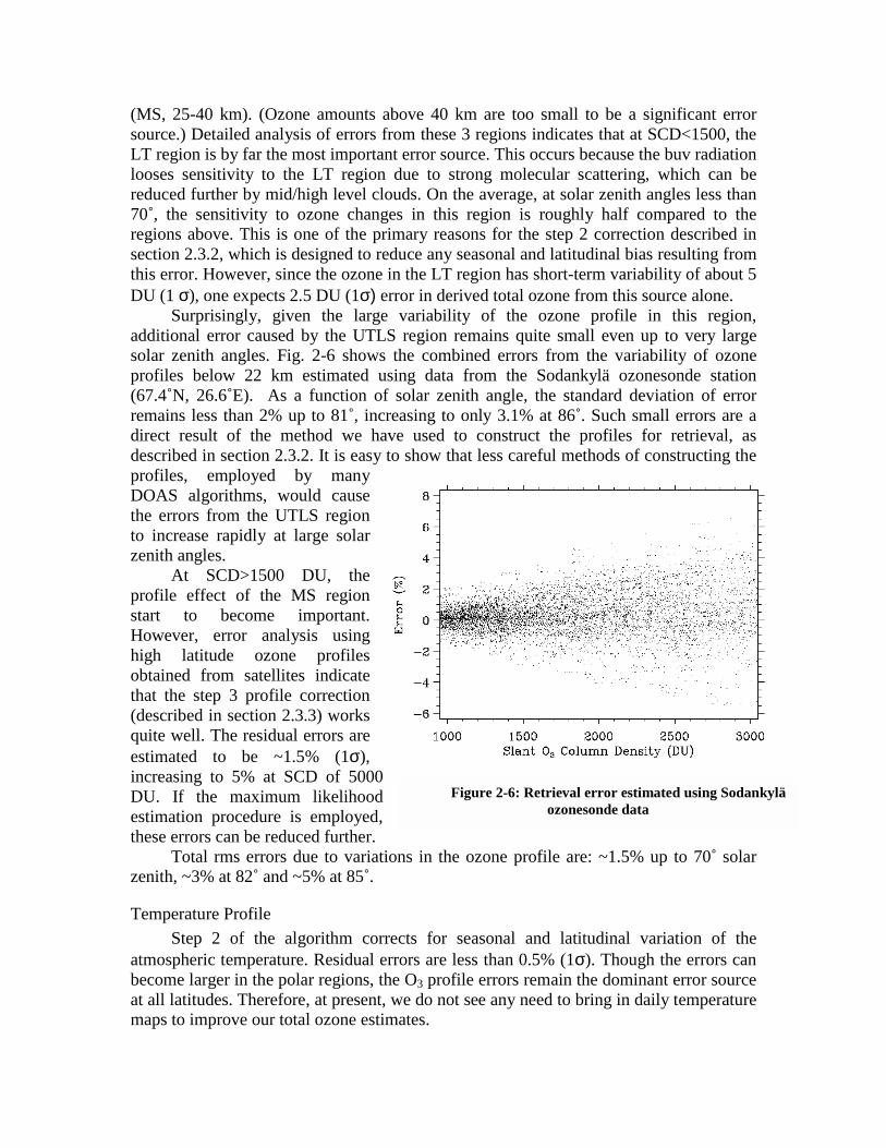
Figure 2-6: Retrieval error estimated using Sodankylä ozonesonde data

(MS, 25-40 km). (Ozone amounts above 40 km are too small to be a significant error source.) Detailed analysis of errors from these 3 regions indicates that at SCD<1500, the LT region is by far the most important error source. This occurs because the buv radiation looses sensitivity to the LT region due to strong molecular scattering, which can be reduced further by mid/high level clouds. On the average, at solar zenith angles less than 70˚, the sensitivity to ozone changes in this region is roughly half compared to the regions above. This is one of the primary reasons for the step 2 correction described in section 2.3.2, which is designed to reduce any seasonal and latitudinal bias resulting from this error. However, since the ozone in the LT region has short-term variability of about 5 DU (1 σ), one expects 2.5 DU (1σ) error in derived total ozone from this source alone.

Surprisingly, given the large variability of the ozone profile in this region, additional error caused by the UTLS region remains quite small even up to very large solar zenith angles. Fig. 2-6 shows the combined errors from the variability of ozone profiles below 22 km estimated using data from the Sodankylä ozonesonde station (67.4˚N, 26.6˚E). As a function of solar zenith angle, the standard deviation of error remains less than 2% up to 81˚, increasing to only 3.1% at 86˚. Such small errors are a direct result of the method we have used to construct the profiles for retrieval, as described in section 2.3.2. It is easy to show that less careful methods of constructing the profiles, employed by many DOAS algorithms, would cause the errors from the UTLS region to increase rapidly at large solar zenith angles.

At SCD>1500 DU, the profile effect of the MS region start to become important. However, error analysis using high latitude ozone profiles obtained from satellites indicate that the step 3 profile correction (described in section 2.3.3) works quite well. The residual errors are estimated to be ~1.5% (1σ), increasing to 5% at SCD of 5000 DU. If the maximum likelihood estimation procedure is employed, these errors can be reduced further.

Total rms errors due to variations in the ozone profile are: ~1.5% up to 70˚ solar zenith, ~3% at 82˚ and ~5% at 85˚.

Temperature Profile Step 2 of the algorithm corrects for seasonal and latitudinal variation of the

atmospheric temperature. Residual errors are less than 0.5% (1σ). Though the errors can become larger in the polar regions, the O3 profile errors remain the dominant error source at all latitudes. Therefore, at present, we do not see any need to bring in daily temperature maps to improve our total ozone estimates.

2.4.3 Instrumental Errors Instrumental errors include systematic errors due to pre-launch errors in instrument

calibration (spectral and radiometric), calibration drift after launch, and random noise. Since we do not yet know how large these errors are likely to be, we provide sensitivity to various errors in the following.

Spectral Calibration The 317.5 nm wavelength is located on a plateau in ozone absorption cross-section,

hence it is not particularly sensitive to wavelength error: 0.01 nm error in wavelength produces 0.1% error in ozone. This is roughly the uncertainty in the TOMS wavelength calibration.

Radiometric Calibration Unlike the DOAS algorithm, the TOMS V8 algorithm is quite sensitive to

radiometric calibration errors. A 1% calibration error, independent of wavelength between 317.5 nm and at 329.3 nm, introduces a 0-2 DU ozone error depending on brightness of the scene. (Larger errors occur for darker scenes.) A 1% relative calibration error between the two wavelengths introduces ~4-6 DU error depending on slant column ozone amount. (Smallest errors occur at SCD of ~1000 DU). Over the years several strategies have been developed to detect the calibration errors by the analysis of residues. We estimate that the radiometric calibration of an individual TOMS is accurate to 1%, and may contain drifts of 1 %/decade or less. This is not currently true of TOMS data after the middle of year 2000 when uncertainties in the EP TOMS characterization become significant.

Instrument Noise A 1% instrument noise at each of the two wavelengths used for total ozone retrieval

would lead to 6-9 DU noise in total ozone. The noise of the TOMS instrument is 3 to 4 times better than this, so its effect will be well below the systematic errors and therefore of little significance.

2.4.4 Error Summary All the important error sources we have discussed above are systematic, i.e., the

errors are repeatable given the same geophysical conditions and viewing geometry. However, most errors vary in a pseudo-random manner with space and time, so they tend to average out when data are averaged or smoothed. The best way to characterize these errors is as follows: the errors at any given location would have a roughly Gaussian probability distribution with standard deviation of about 2% at solar zenith angles less than 70˚, increasing to 5% at 85˚, with a non-zero mean. The means themselves will have a roughly Gaussian distribution with standard deviation of about 1% with non-zero mean of ±2% (due to error in ozone absorption cross-section). Conservatively, one should assume that the latter error distribution is not affected by the amount of smoothing, i.e., it remains the same whether one looks at monthly mean at any given location, daily zonal mean, monthly zonal mean, or even yearly means.

2.6 References Ahmad, Z. and P. K. Bhartia, Effect of Molecular Anisotropy on the Backscattered UV

Radiance, Appl. Opt., 34, 8309-8314, 1995. Bass, A. M. and R. J. Paur, The ultraviolet cross-section of ozone, I, The measurements,

in Atmospheric Ozone, edited by C. S. Zerefos and A, Ghazi, 606-610, D. Reidel, Norwood, Mass., 1984.

Bates, D. R., Rayleigh scattering by air, Planet. Space. Sci., 32, 785-790, 1984. Bhartia, P. K., J. R. Herman, R. D. McPeters and O. Torres, Effect of Mount Pinatubo

Aerosols on Total Ozone Measurements From Backscatter Ultraviolet (BUV) Experiments, J. Geophys. Res., 98, 18547-18554, 1993.

Caudill, T.R., D. E. Flittner, B. M. Herman, O. Torres and R. D. McPeters, Evaluation of the pseudo-spherical approximation for backscattered ultraviolet radiances and ozone retrieval, J. Geophys. Res., 102, 3881-3890, 1997.

Deirmendjian, D., Electromagnetic scattering on spherical polydispersions, Elsevier, 290, 1969.

Greenblatt, G. D., J. J. Orlando, J. B. Burkholder and A. R. Ravishankara, Absorption Measurements of Oxygen Between 330 and 1140 nm, J. Geophys. Res., 95, 18,577-18,582, 1990.

Dave, J. V., Meaning of successive iteration of the auxiliary equation of radiative transfer, Astrophys. J., 140, 1292-1303, 1964.

Dave, J. V. and C. L. Mateer, A preliminary study on the possibility of estimating total atmospheric ozone from satellite measurements, J. Atmos. Sci., 24, 414-427, 1967.

Dave, J. V., Effect of Aerosols on the estimation of total ozone in an atmospheric column from the measurements of its ultraviolet radiance, J. Atmos. Sci., 35, 899-911, 1978.

Eck, T. F., P. K. Bhartia, P. H. Hwang, and L. L. Stowe, Reflectivity of the Earth's Surface and Clouds in Ultraviolet from Satellite Observations, J. Geophys. Res., 92, 4287, 1987.

Fishman, J., P. Minnis, J. Henry, and G. Reichle, Use of satellite data to study tropospheric ozone in the tropics, J. Geophys. Res., 91, 14,451-14,465, 1986.

Herman, B. M., and S. R. Browning, 1965, A numerical solution to the equation of radiative transfer, J. Atmos. Sci., 22, 559-566, 1965.

Herman, J. R., and E. A. Celarier, Earth surface reflectivity climatology at 340-380 nm from TOMS data, J. Geophys. Res.,102, 28003-28011, 1997.

Joiner, J., P. K. Bhartia, R. P.Cebula, E. Hilsenrath, R. D. McPeters, and H. W. Park, Rotational-Raman Scattering (Ring Effect) in Satellite Backscatter Ultraviolet Measurements, Appl. Opt., 34, 4513-4525, 1995.

Joiner, J. and P. K. Bhartia, The Determination of Cloud Pressures from Rotational-Raman Scattering in Satellite Backscatter Ultraviolet Measurements, J. Geophys. Res.,100, 23019-23026, 1995.

Joiner, J. and P. K. Bhartia, Accurate determination of total ozone using SBUV continuous spectral scan measurements, J. Geophys. Res., 102, 12,957-12,970, 1997.

Klenk, K. F., P. K. Bhartia, A. J. Fleig, V. G. Kaveeshwar, R. D. McPeters, and P. M. Smith, Total ozone determination from the Backscattered Ultraviolet (BUV) experiment, J. Appl. Meteorol., 21, 1672-1684, 1982.

Mateer, C. L., D. F. Heath, and A. J. Krueger, Estimation of total ozone from satellite measurements of backscattered ultraviolet Earth radiance, J. Atmos. Sci., 28, 1307-1311, 1971.

McPeters, R. D. et al., Nimbus-7 Total Ozone Mapping Spectrometer (TOMS) Data Products User's Guide, NASA Reference Publication 1384, 1996.

Torres, O., Z. Ahmad and J. R. Herman, Optical effects of polar stratospheric clouds on the retrieval of TOMS total ozone, J. Geophys. Res., 97, 13015-13024, 1992.

Torres, O., J. R. Herman, P. K. Bhartia, and Z. Ahmad, Properties of Mt. Pinatubo Aerosols as Derived from Nimbus-7 TOMS Measurements, J. Geophys. Res., 100, pp. 14,043-14,056, 1995.

Torres, O., P. K. Bhartia, J. R. Herman, Z. Ahmad, and J. Gleason, Derivation of aerosol properties from satellite measurements of backscattered ultraviolet radiation: Theoretical basis, J. Geophys. Res., 103, 17,099-17,110, 1998.

Torres, O. and P. K. Bhartia, Impact of tropospheric aerosol absorption on ozone retrieval from backscattered ultraviolet measurements, J. Geophys. Res., 104, 21569-21,577, 1999.

Voigt, S., J. Orphal, K. Bogumil and J.P. Burrows," The temperature dependence (203-293 K) of the absorption cross sections of O3 in the 230-850 nm region measured by Fourier-Transform spectroscopy, J. Photochem. Photobiol. A, 143, 1-9, 2001.

Wellemeyer, C. G., S. L. Taylor, C. J. Seftor, R. D. McPeters and P. K. Bhartia, A correction for total ozone mapping spectrometer profile shape errors at high latitude, J. Geophys. Res., 102, 9029-9038, 1997.

Ziemke, J. R., S. Chandra and P. K. Bhartia, Two New Methods of Deriving Tropospheric Column Ozone from TOMS Measurements: The Assimilated UARS MLS/HALOE and Convective Cloud Differential Technique, J. Geophys. Res., 103, 22,115-22,127, 1998.