INSIGHTS FROM THE DOWNHOLE DYNAMOMETER DATABASE

John R. Waggoner Sandia National Laboratories Albuquerque, New Mexico I

Abstract The Downhole Dynamometer Database is a compilation of test data collected with a set of five

downhole tools built by Albert Engineering under contract to Sandia National Laboratories. The downhole dynamometer tools are memory tools deployed in the sucker rod string with sensors to measure pressure, temperature, load, and acceleration. The acceleration data is processed to yield position, so that a load vs. position dynagraph can be generated using data collected downhole. With five tools in the hole at one time, all measured data and computed dynagraphs from five different positions in the rod string are available.

The purpose of the Database is to provide industry with a complete and high quality measurement of downhole sucker rod pumping dynamics. To facilitate use of the database, Sandia has developed a Microsoft Windows-based interface that functions as a visualizer and browser to the more than 40 MBytes of data. The interface also includes a data export feature to allow users to extract data from the database for use in their own programs,

Following a brief description of the downhole dynamometer tools, data collection program, and database content, this paper will illustrate a few of the interesting and unique insights gained from the downhole data.

DISCLAIMER

This report was prepared as an account of work sponsored by an agency of the United States Government. Neither the United States Government nor any agency thereof, nor any of their employees, makes any warranty, express or implied, or assumes any legal liability or responsi- bility for the accuracy, completeness, or usefulness of any information, apparatus, product, or process disclosed, or represents that its usc would not infringe privately owned rights. Refer- ence herein to any specific commercial product, process. or service by trade name, trademark, manufacturer, or otherwise dots not necessarily constitute or imply its endorsement, m m - mendation, or favoring by the United States Government or any agency thereof. The views and opinions of authors exprcssed herein do not necessarily state or reflea thosc of the United States Government or any agency thereof.

This work was supported by the United States Department of Energy under Contract DE-AC04- 94AL85000. Sandia is a multiprogram laboratory operated by Sandia Corporation, a Lockheed Martin Company, for the United States Department of Energy.

Portions of this document may be rUegible in electronic image products. Images are produced from the best avaiiable original document.

Introduction The Downhole Dynamometer Database (DDDB) is a compilation of test data collected by Sandia

National Laboratories (SNL) using downhole dynamometer tools built by Albert Engineering (AE). The purpose of the DDDB is to provide industry with a complete and high quality measurement of downhole sucker rod pumping dynamics. To facilitate use of the DDDB, Sandia developed a Microsoft Windows- based interface that functions as a visualizer and browser to the more than 40 MBytes of data. The interface also includes a data export feature to allow users to extract data from the database for use in their own programs. A description of the downhole dynamometer tools’ and database2 have been published previously, so this paper only briefly summarizes these topics before presenting selected downhole dynamometer data from the database to illustrate the content of the database and suggest the utility of the data.

Database Interface The DDDB Interface program, DownDyn, is a Microsoft Visual Basic version 3.0 program that

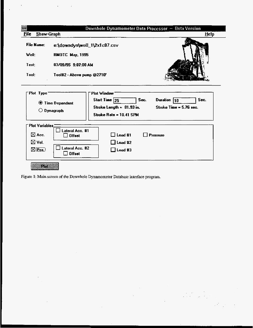
runs on Microsoft Windows 3.11, Windows 95 (not tested), and Windows NT. Figure 1 shows DownDyn’s main screen. The program includes graphing utilities necessary to generate and display plots. Instructions for installation and how to import user data for viewing, or add user data to the database, are contained in a readme.txt file. Other help information is contained in the help facility built into the program. Current information about the status of the database and interface can be found at http://www. sandia. gov/apt/.

The DDDB Interface performs four functions: selecting a data file, choosing information from the file, plotting, and importing/exporting information. Data files are selected by scrolling through lists of the wells in the database and of the tests performed on each well. If the data file chosen is for a surface dynamometer test, there is no information that must be selected before plotting. If the data file chosen is a downhole test, there are a number of choices to be made before plotting, such as the Plot Type, Plot Variables, and Plot Window.

Once a plot is displayed, it can be printed or copied, or its data can be exported to a file as comma delimited columnar ASCII data. Imported/exported dynagraph data may conform to either Nabla’s or Theta Enterprises’ dynamometer file format. Downhole time dependent data is stored as comma delimited data and must have the extension “,csv”. Data files, including all raw data files, can be accessed via standard DOS or Windows File Manager commands. This functionality opens the DDDB for direct access by the user if, for example, the user’s plotting needs exceed the capability of the DDDB Interface program. This also allows the user to process the data differently, such as using sophisticated signal processing software to gain insight into the nature of the data recorded, and then filter the data to focus on a particular feature of interest.

The Downhole Dynamometer Tools The downhole dynamometer tools are memory tools deployed in the sucker rod string with sensors

to measure pressure, temperature, load, and acceleration.’ Load is measured with three full bridge strain gages located at 120” intervals on the ID of the housing. The three load readings average to equal the rod load, and differences between the three load readings gives an indication of rod bending. Acceleration is measured with three separate orthogonal piezoresistive accelerometers with one accelerometer positioned along the axis of the tool. The axial accelerometer data is integrated twice to yield the position of the tool as a function of time, while data from the other two accelerometers gives an indication of the lateral motion of the tool. The sensors are housed in a 12” long by 1.75” OD pump barrel with 0.75” API pin couplings on each end. The housing has been pull tested to failure at 39,600 lbf tension.

The Data Collection Program Data for the DDDB was collected in a cooperative effort between SNL and the petroleum industry.

For each test, a producing company provided the well and pulling crew, Sandia provided the tools, and, except for the Wyoming test, Nabla provided the surface data collection. The identity of the producing company has been removed from the DDDB to protect their interests, again except for the Wyoming test conducted with the DOE’s Rocky Mountain Oilfield Testing Center (RMOTC) near Casper, WY.

Database Content The DDDB contains six tests, although downhole data from only 4 of those are available at the time

this paper is being written. All the data should be available when the database is released. The six tests are described below in the Insights section along with some comments on the data itself. Each test contains the measured downhole data processed by Albert Engineering to also generate velocity and position data derived from the measured acceleration data. For archival purposes, the database also includes the raw datafiles delivered by AE for each test, but this information is not available through the interface program.

The database also contains a description file for each test that provides detailed inforrnation including tool locations, pumping unit, rod string taper, and production data. In addition to data collected with the downhole tools, the DDDB contains surface data collected by Nabla, except for the first test in Wyoming where the surface data was collected by RMOTC using Delta-X equipment. By including the surface data in the DDDB, users are able to download this information into their own diagnostic software and compare the results with data measured downhole. This comparison is beyond the scope and intent of this project and is not included in the DDDB.

Insights The primary intent of the project was to provide a tool that the industry could use to gain insight

into the downhole dynamics of sucker rod pumping. As such, little effort has been made at Sandia to analyze the data. However, presented here are some interesting features of the data as noted while assembling the DDDB. Any significance attributed to these features will need to be assigned by industry.

1) 2700’ well at DOE’s Rocky Mountain Oilfield Testing Center near Casper, Wyoming. This 2700’ well has a 0.75” API Grade ‘C’ steel rod string with a 1.5” RWA pump in 2.875” tubing. The well produces about 4 BOPD of 38 degree API oil, 130 BWPD, and no gas, while pumping at about 11 SPM with an 86” surface stroke. Tools were located:

1) below the pump (failed, no data), 2) above the pump at 2710’, 3) at 2462’, 4) at 1003’, and 5) below the polished rod.

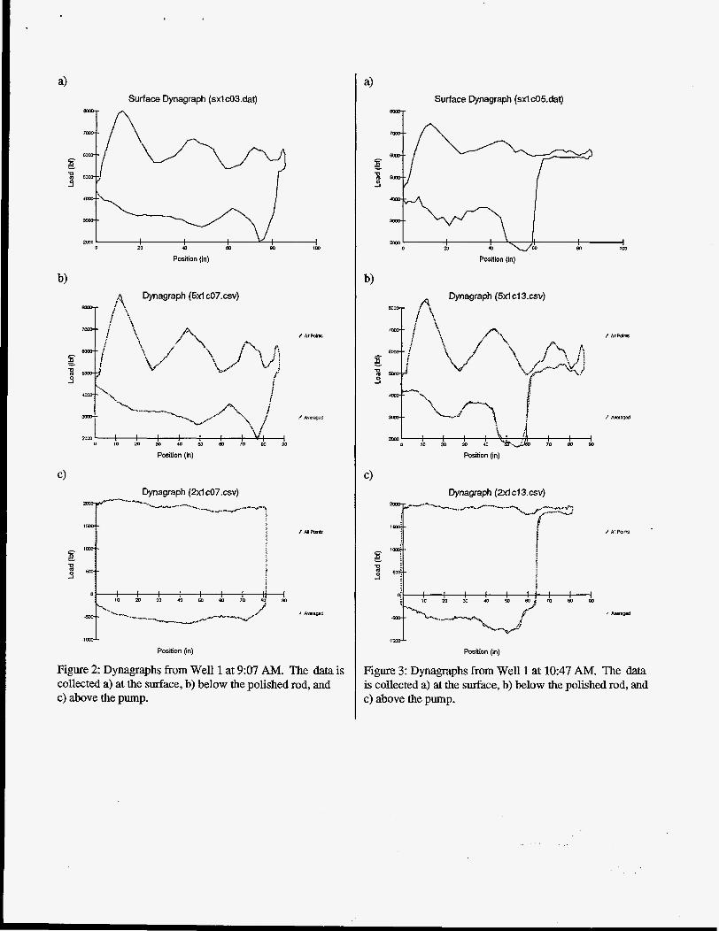
This well was chosen to be fairly representative of a large number of ‘normal’ wells, if there is such a thing. In addition to the data, the test provided confidence that the tools were functioning well and were durable enough to survive downhole conditions. The well produced continuously during the test with no intended changes to the operation of the well, and no prior indication that the well would pump-off. Figure 2 shows a series of dynagraphs taken at 9:07 AM on the first day of the test, showing a full pump card at the bottom, Fig. 2c, and good agreement between the surface card, Fig. 2a, and the card acquired below the polished rod Fig. 2b.

Just one and a half hours later, at 10:47 AM, dynagraphs clearly show, Fig. 3, a pumped-off condition that was not expected. Again there is similarity between the surface and near-surface cards, Figs. 3a and 3b, respectively, but the higher sampling rate of the downhole tools shows more detail in the card. The next recording period at 11:07 AM, not shown, is similar to the 9:07 AM period,

indicating that reservoirs anc, wells are dynamic, and that there is benefit to continuous, or at least frequent, monitoring of wells. Automatic pump-off controllers are one means of adjusting to the dynamic and irregular behavior of reservoirs and wells.

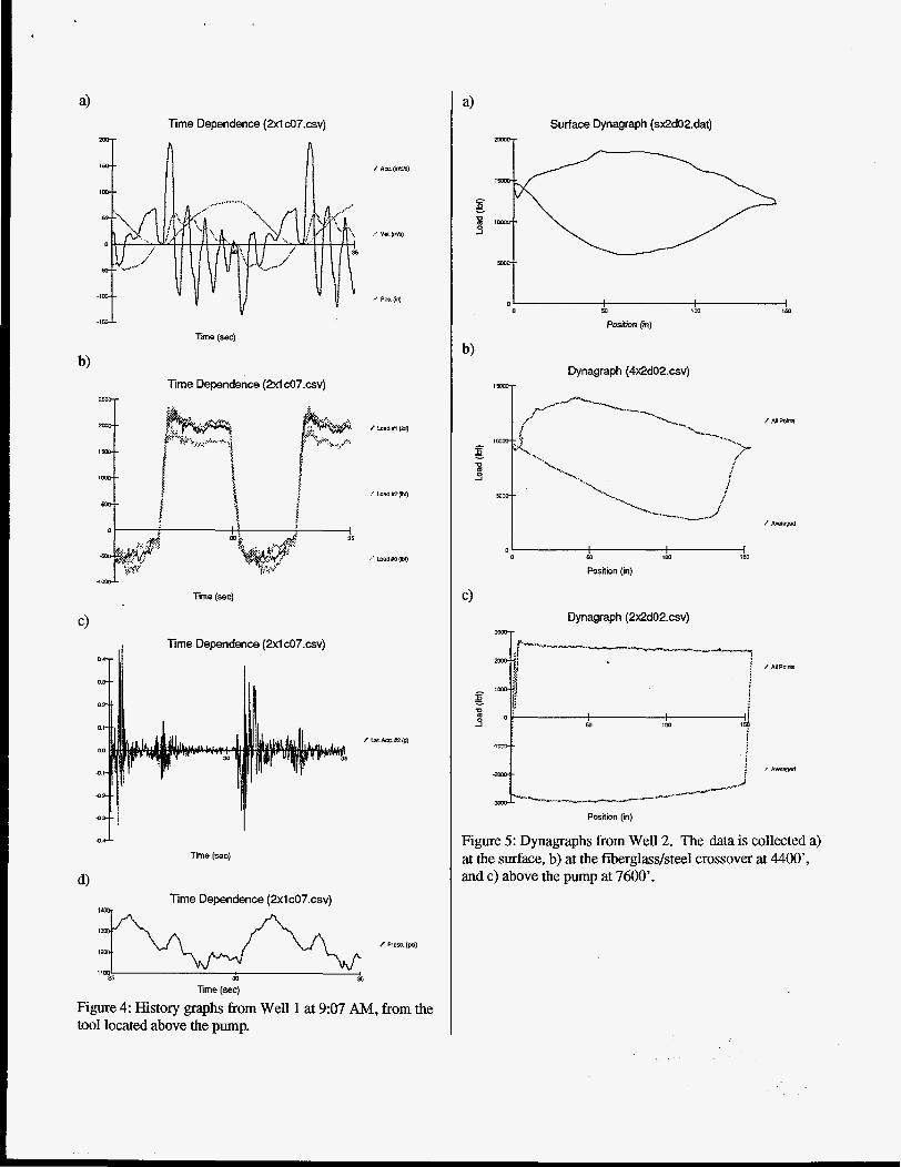
Figure 4 shows a group of time dependent plots from the tool above the pump at the 9:07 AM recording period to illustrate some of the other types of information in the database. Figure 4a shows axial acceleration, velocity, and position for 10 second in the middle of the one minute recording interval. While the position curve looks relatively smooth, the acceleration and velocity curves are not. Since this tool is very close to the pump plunger, this suggests that the pump action is not as smooth as expected. This variation in plunger acceleration and velocity is probably related to the propagation of stress waves in the rod string as indicated by the regular spacing of the acceleration peaks.

Figure 4b shows the three load signals reading the axial load on the tool. With the three load gages positioned 120 degrees apart from each other, separations between the three signals indicate bending moments applied to the tool. In this case, bending indicated on the upstroke may be caused by hole deviation or off-axis threading of the coupling joining the tool to the sucker rod string. Bending indicated on the downstroke is more interesting, however, because it changes in both magnitude and direction during the downstroke, indicating dynamic behavior. The three curves agree well in the beginning of the downstroke, indicating that there is no bending, but then diverge toward the middle of the stroke to indicate bending. The interesting feature in the middle of the stroke is that the direction of bending changes, indicated by the change in the relative position of the three curves. This could be caused by buckling, or at least an instability leading to horizontal motion of the tool.

This thesis is supported by Fig. 4c showing one of the lateral acceleration curves, which shows an increase in lateral, or horizontal, motion during the middle of the downstroke. The magnitude of the lateral acceleration is not large, but is clearly greater than during the upstroke. This data needs to be analyzed to determine what magnitude of lateral acceleration would indicate that the tool is banging against the tubing, either at this tool or somewhere else in the string with the resulting shear wave propagating to this tool.

Figure 4d in this figure shows the fluid pressure measured during the interval. Without any prior notion of what the pressure should look like, it is hard to say that this is interesting behavior. However, it clearly indicates that the hydraulics of the pump stroke, in this case looking only at the output of the pump, is very complicated and could impart additional dynamic compressive loading on the rod stsing. This complexity also impacts the design and diagnostic codes which may assume a more static pressure condition at this lower boundary of their wave equation model. Further study is warranted here as well.

2)7600’ well with a mixed fiberglasshteel rod string. This 7600’ well has 4400’ of 1.125” Noms fiberglass rods, 3200’ of 1” API Grade ‘D’ steel rods, and a 1.5” insert pump in 2.875” tubing. The well produces about 29 BOPD of 40 degree API oil, 210 BWPD, and a GOR of 1620 when pumped at 8.2 SPM with a 144” surface stroke. With the tubing anchor set at 6168’ and the seating nipple at 7655’, almost 1500’ of tubing below the anchor is subject to stretch. A shallow rod part early in the test schedule terminated the test after only one downhole test period and one surface measurement. Tools were located:

1) below the pump, 2) above the pump at 7600’, 3) 75’ above the pump in the 1” rods, 4) at 4400’ at the fiberglass/steel crossover, and 5) 75’ above the crossover.

This well was chosen to examine the effect of fiberglass rod strings under different pumping conditions, especially to provide measured data to design and diagnostic code developers to check their fiberglass string model. Unfortunately, only one recording period was captured before the rods

parted and terminated the test. It is useful to note that the tools appeared to sustain no damage caused by the part or subsequent fishing job.

Figure 5 shows the series of dynagraphs collected. The surface card, Fig. 5a, was collected at 9:35 AM, while the downhole measurements were taken at 6:47 AM, so they are not coincident in time as on the other figures. The pump card, Fig. 5c, shows almost 3000 lbf compression on the downstroke which agrees well with the Nabla predicted pump card when likely rodtubing friction is taken into account. Tools 4 and 5 were located 75’ apart at the bottom of the fiberglass portion of the string to allow comparison of closely space measured data.

suggesting the possibility that tubing movement could affect the performance of the pump. Figure 6 shows graphs for position and axial acceleration for a tool located below the pump, and indicates that the bottom of the tubing moved about 2.5” during the pump stroke. The acceleration curve shows a great deal of variation at the beginning of the upstroke, leading to the ‘V’ feature at about 27 sec. It is interesting to note that this motion is not in-phase with the plunger motion as indicated by the position and axial acceleration graphs for the tool located above the pump, as shown in Fig. 7. These tools are synchronized in time such that an event recorded on one tool at 30 sec., for example, occurs at the same time as a measurement on another tool at 30 sec. While there is some drift in the tools’ clocks, it can be considered negligible relative to one another.

The character of the two position curves in Figs. 6 and 7 suggests that different mechanisms confrol the motion of the tools. It is interesting that the plunger reaches it’s lowest point at the same time, about 27 sec., as the bottom tool reaches it’s highest point, at which the aforementioned ‘V’ feature occurs. Since the tool below the pump is directly attached to the standing valve, could this indicate that the plunger is tagging the standing valve at this point? There was no surface indication of tagging, so there may not be a detrimental effect of the tagging if it is indeed occurring.

Another interesting feature of this well is that the bottom 1500’ of tubing is not anchored,

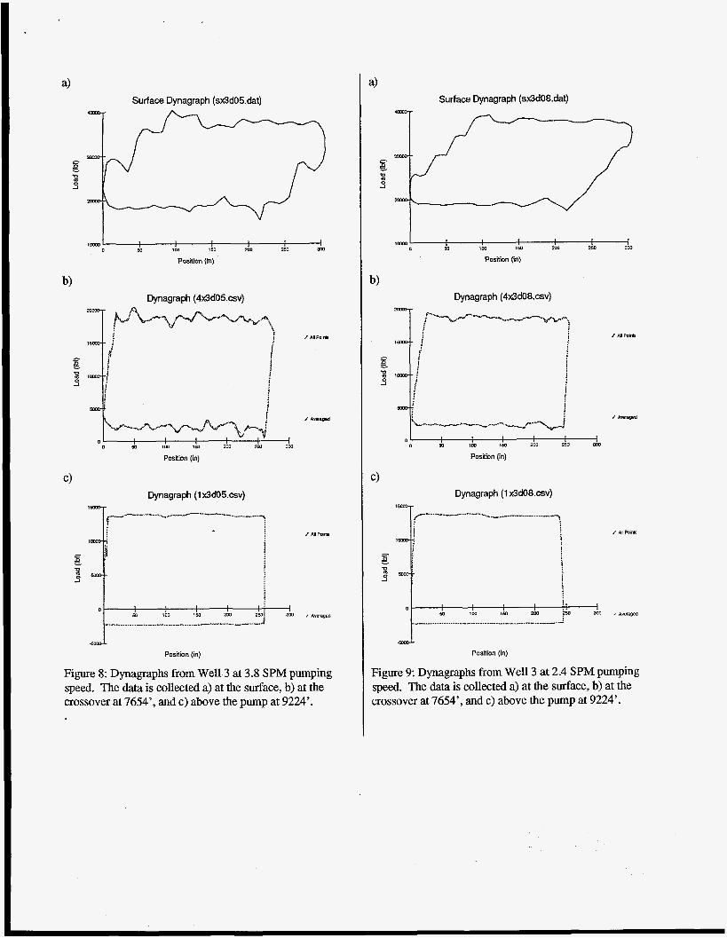
3)9300’ well with a Rotaflex pumping unit. This 9300’ well has an API Grade ‘D’ steel rod string made of 3329’ of 1” rods, 4325’ of 0.875” rods, and 1525’ of 1” rods on bottom. The 2.25” diameter tubing pump in 2.875” tubing produces about 28 BOPD of 34 degree API oil, 447 BWPD, and no measured gas, when pumped 3.9 SPM with a 306” surface stroke. The Rotaflex pumping unit had a variable frequency drive that was operated at 3.8,3.5,2.9, and 2.4 SPM to measure the dynamics of the Rotaflex unit at different speeds. Tools were located:

1) above the pump at 9224’, 2) at 9082’ in 1” rods, 3) at 8780’ in 1” rods, 4) at 7654’ at the lower 0.875” rod/l” rod crossover, and 5) at 7500’ in the 0.875” rods.

This well was chosen to investigate the dynamics introduced into the rod string by the rapid direction changes characteristic of the Rotaflex pumping unit. The producing company was particularly interested in the effect of rate on the dynamics to see if an optimal pumping rate to avoid rod failures could be determined. Figures 8 and 9 show dynagraphs for 3.8 and 2.4 SPM pumping speeds, respectively. There does not appear to be much difference between the loads or shapes of the cards, but the downhole stroke length is about 5% longer at the faster pumping speed. With the sharp transitions observed at the corners of the cards, it may be necessary for sucker rod codes to use higher precision numerical methods when modeling a Rotaflex well than a more conventional well.

Figures 10 and 11 show groups of time dependent plots for 3.8 and 2.4 SPM pumping speeds, respectively. Figures 10a and 1 l a show axial acceleration, velocity and position for slightly more than a stroke near the middle of the one minute recording interval. The position curve for this Rotaflex unit is noticeably more abrupt in transition than is a conventional unit, as shown for example in Fig. 4a, and this characteristic is the same at either speed. However, the axial acceleration appears to show more frequent and larger magnitude harmonics at the higher speed.

Figures 10b and 1 l b show the three load signals, which show very little difference at the two speeds. Both graphs indicate bending on the upstroke that changes during the upstroke. This feature suggests lateral motion of the tool, which is supported by Figs. 1Oc and 1 IC showing lateral acceleration. At the higher speed, Fig. lOc, higher magnitude spikes in the acceleration, as compared to the lower speed, Fig. 1 IC, suggest more severe lateral motion, although there is still a considerable amount of motion at the lower speed. Again comparing these Rotaflex curves to the conventional curves in Fig. 4c, the acceleration appears to be an order of magnitude greater for the Rotaflex. There is not enough evidence to say that this is a result of the Rotaflex unit since there are a considerable number of other differences between the wells, such as depth, but it is possible that the Rotaflex unit introduces this behavior. Again, the significance of this occurring, if it does, will need to be established in a future study.

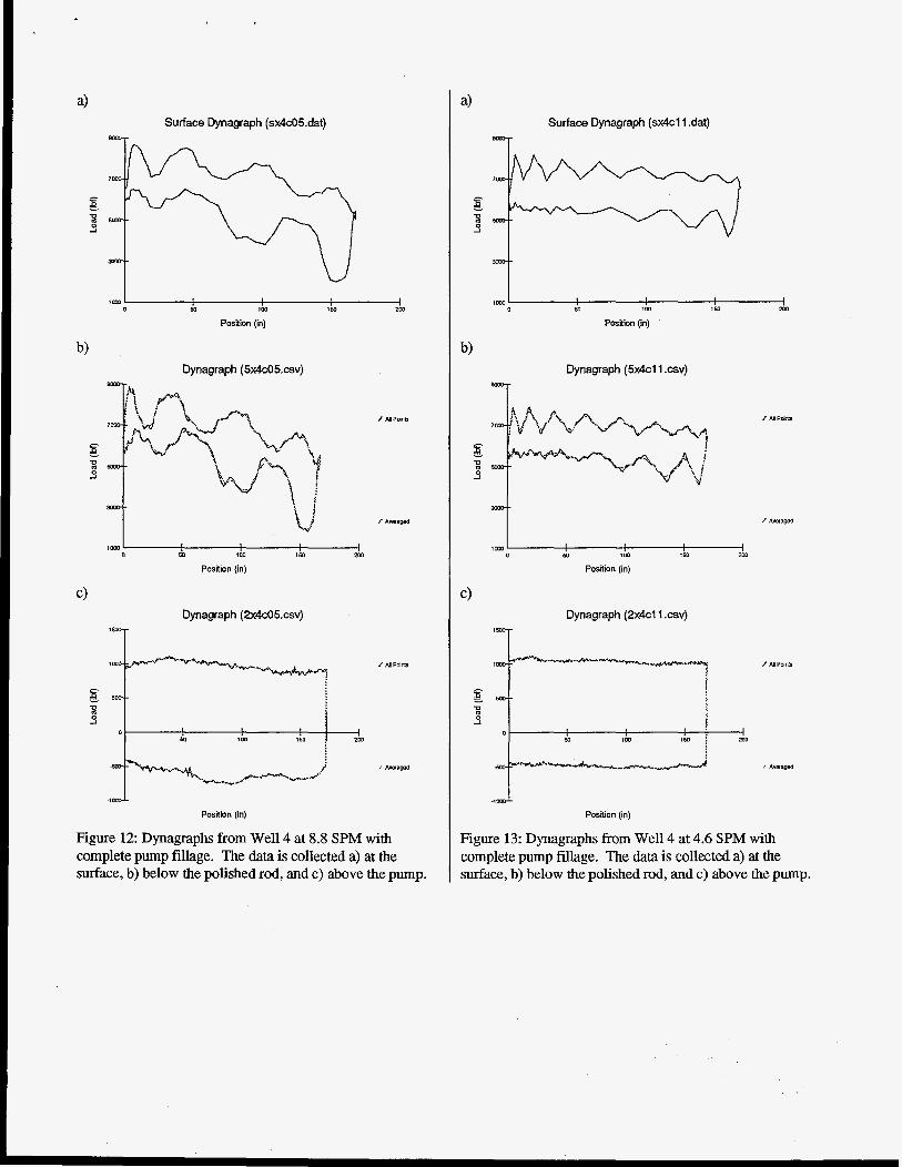
4)2600’ well with varied pump speed and fillage. This 2600’ well has an API Grade ‘D’ steel rod string made of 1002’ of 0.875” rods, 1700’ of 0.75” rods, and 300’ of 1.25” sinker bars. A bridge plug above the perforations allows the pump fillage to be controlled by the rate of water entering the annulus from a frac tank at the surface. The 1.25” insert pump in 2.875” tubing produces 140 BWPD when pumped at 4.6 SPM with a 168” surface stroke. By changing the sheaves on the pumping unit, pumping speeds of 8.8,6.7, and 4.6 SPM were obtained. Tools were located:

1) below the pump, 2) above the pump, 3) at 1702’ at the bad0.75” rod crossover, 4) at 1002’ at the 0.75” rod/0.875” rod crossover, and 5 ) below the polished rod.

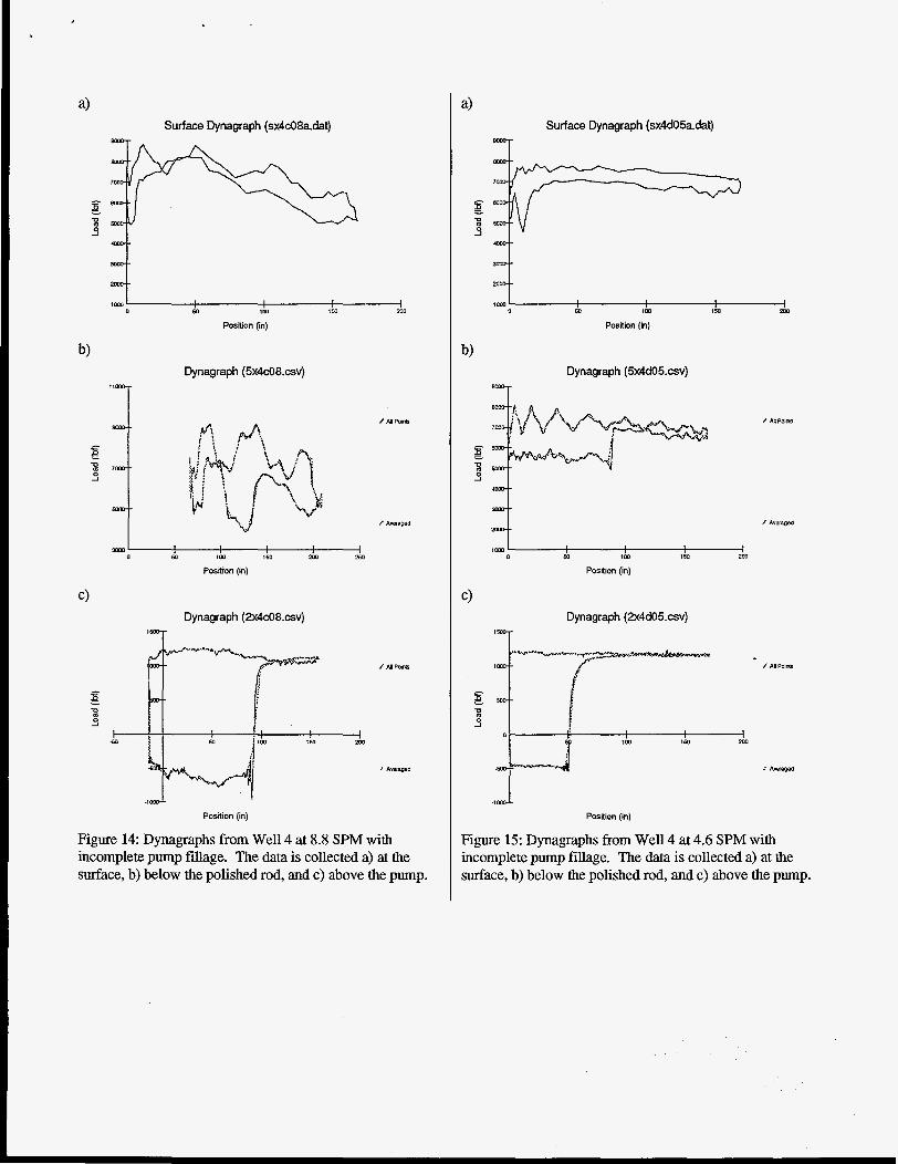
This well was chosen and configured as a controlled test well to study the combined effects of pumping speed and pump fillage on sucker rod dynamics. Figures 12 and 13 show dynagraphs for 8.8 and 4.6 SPM pumping speeds, respectively, with a full pump. The slower speed appears to produce more regular cards with less compression on the downstroke. Figures 14 and 15 show dynagraphs for 8.8 and 4.6 SPM pumping speeds, respectively, with incompletely filled pumps.

It is important to note that, while the downhole tools are synchronized to collect data at the same time, the surface dynamometer is synchronized to take data not at the same time, but during the same one minute interval that the downhole tools are collecting dak- This is not a problem in the full pump measurements because it was fairly easy to establish a uniform pumping condition over the one minute recording interval, so that a stroke early in the interval would look very much like a stroke later in the interval.

However, in the incomplete fillage cases, it was very difficult, if not impossible, to establish a uniform pumping condition over the one minute recording interval, so each stroke during the interval can look very different. This problem is illustrated in Fig. 15 where the pump card, Fig. 15c, indicates about 30% fillage, the card from tool 5 located below the polished rod, Fig. 15b, indicates about 50% fillage, but the surface card, Fig. 15a, indicates only about 10 - 15% fillage. Clearly data collected in this non-uniform way adds uncertainty about any comparisons, but it should be possible to export the tool 5 card from the database and use it in diagnostic programs as if it were collected at the surface. This adds to the utility of placing a tool below the polished rod. Comparing these results to the downhole cards should then be valid and insightful. In addition, analyzing the other downhole data, such as acceleration, pressure, and load, as functions of time may indicate interesting dynamics not seen in, or predicted from, the surface measurements.

It is also theoretically possible to adjust the start time for these dynagraphs until the tool 5 card matches the fillage indicated on the surface card, thus approximately establishing the desired time synchronization between the surface and downhole measurements. However, there is difficulty in moving the start time to the extremes of the recording interval, as illustrated in Fig. 14. Figure 14b shows a tool 5 dynagraph using a start time of 43 sec. (all other dynagraphs in this paper were

generated using a default start time of 25 sec.), and is clearly NOT a good representation of the load vs. position behavior of the rod string below the polished rod. What happened? The problem lies with the position data, not the load data. In fact, there is not a problem with any of the measured data (position is derived, not measured), so, even when dynagraphs are in error, all the measured time- dependent data is still valid.

Figure 16 shows position data over the one minute recording interval corresponding to Fig. 14b, and indicates considerable ‘drift’ in the position data. Since the tool is constrained to move within a fixed range of positions in the rod string, this ‘drift’ is clearly non-physical. The problem arises when small errors, or transducer drift, in the measured axial accelerometer data are magnified by the process of integrating the data twice to generate position data. AE chooses the integration constants to optimize the position data at the center of the recording interval, which results in poor position data at the extremes of the recording interval. Attempts at Sandia to eIiminate this problem, such as higher order integration, frequency domain integration, and low pass filtering, have resulted in some improvement, but have not succeeded in eliminating the problem. Other approaches that operate on only a portion of the data at a time, such as a stoke-by-stroke procedure, need to be investigated. This problem makes it difficult to adjust the start time enough and still generate valid dynagraphs.

5)5000’ well with Echometer’s decentralized gas separator. This 5000’ well has an API Grade ‘D’ steel rod string made of 1512’ of 1” rods, 1600’ of 0.875” rods, 1625’ of 0.75” rods, and 250’ of 1.5” sinker bars. The 2.0” RWB pump with a hollow pull tube in 2.875” tubing produces about 71 BOPD of 35 degree API oil, 342 BWPD, and 397 MSCFPD of gas (88% CO,), for a GOR of 5592. The well was pumped at 6.5 SPM with a 168” surface stroke. After producing with no gas separator, the well was pulled to install Echometer’s decentralized gas separator, allowing a comparison of the downhole data with and without the gas separator. Tools were located:

(with gas separator) 1) below the pump (failed, no data), 2) above the pump, 3) at 4737’ at the 0.75” rodbar crossover, 4) at 3 112’ in the 0.875” rod/0.75” rod

crossover (failed, partial data), and 5) at 1512’ at the 1” rod/0.875” rod

crossover.

(without gas separator) 1) below the pump (failed, no data), 2) above the pump, 3) at 4737’ at the 0.75” rod/bar crossover, 4) at 4712’ in the 0.75” rods, and 5) below the polished rod

This well was chosen to determine the effectiveness of the decentralized gas separator, but a good comparison may not be possible. This well exhibited unpredictable slugs of gas production that caused the well to flow, so that similar well conditions with and without the separator may not be available. This data has not yet been added to the database.

6)2900’ well with Axelson’s new tension pump. This 2900’ well has 2350’ of 0.875” Nonis 97 steel rods and 500’ of 1.5” sinker bars in 2.875” tubing. Axelson’s new tension pump, with an equivalent plunger diameter of 1.87”, was installed in the early part of the test, and then exchanged for a 2” tubing pump later in the test. The well produces about 10 BOPD of 33 degree API oil, 300 BWPD, and negligible gas when pumped at 7 SPM with a 143.5” surface stroke. Tools were located:

1) below the pump, 2) above the pump (failed, no data), 3) 75’ above the pump in the bars, 4) at 2350’ at the rod/bar crossover, and 5) below the polished rod.

This well was chosen to determine the effectiveness of a tension pump designed to minimize or eliminate compressive loads on the downstroke. This data is not yet available.

Conclusions 1. The downhole dynamometer is a valuable tool in accurately diagnosing downhole sucker rod

2. The downhole dynamometer database contains data that will allow industry to improve predictive and

3. Continuous, or at least frequent, monitoring of wells is needed to capture the dynamic behavior of

4. Pressure measurements indicate complex behavior that is not well modeled by static pressure

5. Unanchored tubing motion does not move in phase with the pump stroke, possibly leading to

6. Calculating position from acceleration data is very sensitive to drift in the measured data. 7. Placing multiple downhole dynamometer tools in the well, including one below the polished rod if

behavior.

diagnostic codes, and develop improved field practices.

wells and reservoirs.

assumptions.

decreased spacing, or even tagging, in some cases.

possible, is needed to fully understand downhole dynamics and protect against loss of data. ’

References 1. Albert, G.: “Downhole Dynamometer Tool,” Proceedings of the Forty-First Annual Meeting of the

Southwestern Petroleum Short Course, Lubbock, TX, April 20-21, 1994. 2. Waggoner, J.R. and Mansure, A. J.: “Development of the Downhole Dynamometer Database,” SPE

37500 presented at the SPE Production Operations Symposium, Oklahoma City, OK, March 9-11, 1997.

Acknowledgments The author gratefully acknowledge the support of Nabla, RMOTC, and the producing companies

that participated in these field tests. In addition, the guidance of the Sucker Rod Working Group, including beta testing by some of the members, is appreciated. The intedace program, DownDyn, was written by A.J. Mansure at Sandia. This work was supported by the United States Department of Energy under Contract DE-AC04-94AL85000. S andia is a multiprogram laboratory operated by Sandia Corporation, a Lockheed Martin Company, for the United States Department of Energy.

- File Show-Graph - Help

File Name:

Well:

Test:

Tool:

e:\d own dyn{welI-l{2xl GO 7. csv

RMDTC May. 1995

03109195 9:07:00 AM

Tool#2 - Above pump e271 0'

r Plot Type 7 r Plot Window 1 @ Time Dependent

0 Dynagraph

Start Time 7 1 Sec-

Stroke Length = 81.93 in.

Stroke Rate = 10-41 SPM

Duration 7 1 Sec.

Stroke Time = 5.76 sec.

Load #2

Load #3

Figure 1: Main screen of the Downhole Dynamometer Database interface program.

Surface Dynagraph (sxlcO3.dat)

s - U

3

D m 6n Bo rm

Position (in)

Dynagraph (5x1 cO7.csv)

- e U

3

/ AbPmm

I Avssged

Position (in)

Dynagraph (2x1 cO7.csv) .-4-I.--..’---_e_T/-,---&

: AYBI.Qed

Position (in)

Figure 2 Dynagraphs from Well 1 at 9:07 AM. The data is collected a) at the surface, b) below the polished rod, and c) above the pump.

Surface Dynagraph (sxl Ca5.dat)

Position (in)

Dynagraph (5x1 d 3 . ~ 5 ~ )

T A.

Dynagraph (2x1 ~13.~5~)

Position (in)

Figure 3: Dynagraphs from Well 1 at 10:47 AM. The data is collected a) at the surface, b) below the polished rod, and c) above the pump.

Time Dependence (2x1 cO7.csv)

b)

d)

Time (sec)

Time Dependence (2x1 cO7.csv)

Time (sec)

O h li Time Dependence (2x1 cO7.csv)

I Time (sec)

Time Dependence (2x1 cO7.csv)

mme (sec)

Figure 4: History graphs from Well 1 at 9:07 AM, from the tool located above the pump.

Surface Dynagraph (sSd02.dat)

0 0

I 5D 100 I 5 0

Position (in)

Dynagraph ( 4 ~ 2 d 0 2 . c ~ ~ )

0 I 0 50 im 150

Posirion (in)

: .. A”6lSgsd i

--------A -.. --.-.-rCCI--/ ------r c

Position (in)

Figure 5: Dynagraphs from Well 2. The data is collected a) at the surface, b) at the fiberglass/steel crossover at MOO’, and c) above the pump at 7600’.

Time Dependence ( l x 2 d 0 2 . c ~ ~ )

Time (sac)

Time Dependence (1 d d 0 2 . w )

Time (sec)

Figure 6: History graphs from Well 2 from tool located below the pump.

Time Dependence ( 2 ~ 2 d 0 2 . s ~ )

25 ZB 21 28 28 30 31 8 3) 34 35

/ Poll (L"]

Time (sec)

Time (sec)

Figure 7: History graphs from Well 2 from tool located above the pump.

Surface Dynagraph (sx3d05.Qt)

E -0

3

I 0 1m 150 m 26.3 300

1m 50

Position (in)

r Avsagsd

50 tm 150 200 291 300

Position (in)

Dynagraph (1 x3d05.c~~)

7 -.

doDDL Position (in)

Figure 8: Dynagraphs from Well 3 at 3.8 SPM pumping speed. The data is collected a) at the surface, b) at the crossover at 7654’, and c) above the pump at 9224’.

i / AUPmre i 1 i

i I

j

Surface Dynagraph (sx3d08.dat)

I 0 6n tm 150 200 250 300

1Oan

Posiiion (in)

b) Gynagraph (4x3d08.e~)

,m 1 9 1 an 250 300

Position (in)

Dynagraph (1 x3d08.c~~)

\__.--- ...__-. I ! i

I Al Pam

I AU PmrW

Posaion (in)

Figure 9: Dynagraphs from Well 3 at 2.4 SPM pumping speed. The data is collected a) at the surface, b) at the crossover at 7654’, and c) above the pump at 9224’.

Time Dependence (Ix3d05.c~~) ,/--

i / A a ( I W )

i

Time (sec)

b) Time Dependence (lx3d05.c~~)

Time (sec)

Time Dependence (1 x3d05.c~~)

Time (sec)

Time Dependence ( lx3d05.c~~)

Time {sec)

Figure 10 History graphs from Well 3 at 3.8 SPM pumping speed, from the tool located above the pump at 9224'.

a) Time Dependence (1 x3dOS.c~~) ).... ,. L.

I A a [ t m n ) '... .i

\

I i

., VM. [am)

... Pai.(m)

-5

Time (sec)

b) Time Dependence (1 x3dOS.c~~)

- 5 O d

Time (sec)

4 Time Dependence (lx3dOS.c~~)

3 Time (sec)

d) Time Dependence (1 B d 0 8 . c ~ ~ )

uah

25 40 55

Time (sec)

Figure 11: History graphs from Well 3 at 2.4 SPM pumping speed, from the tool located above the pump at 9224'.

Surface Dynagraph (sx4d)S.dat)

Position (in)

Dynagraph (5x4c05.c~~)

I I n 50 tM 150 m

Position (in)

Dynagraph (2x4c05.c~~)

r Amaged

I A! Poim

: Averaged

Posiliin (in)

Figure 12: Dynagraphs from Well 4 at 8.8 SPM with complete pump fillage. The data is collected a) at the surface, b) below the polished rod, and c) above the pump.

Surface Dynagraph (sx4cl1 .dat)

PXT-

I 50 ,OD 150 zm

1mO

Position (in)

Dynagraph (5x4~11 .csv)

goo Ea Posaion (in) rm

/ Amaged

Dynagraph (2x4~11 .csv)

.' Avslaged

Figure 13: Dynagraphs from Well 4 at 4.6 SPM with complete pump fillage. The data is collected a) at the surface, b) below the polished rod, and c) above the pump.

Surface Dynagraph (sx4dBa.dat)

- E U

4

0 a I W 150 200

Posli in (in)

Dynagraph (5x4c08.c~~)

0 I

50 I(x1 150 200 250

Position (in)

Dynagraph ( 2 x 4 ~ 0 8 . ~ ~ ~ )

Position (in)

Figure 14: Dynagraphs from Well 4 at 8.8 SPM with incomplete pump fillage. The data is collected a) at the surface, b) below the polished rod, and c) above the pump.

Surface Dynagraph (sx4d05a.dat)

Dynagraph (5x4d05.c~~)

50 iw 150 am

Position (in)

e 2 4

0 50 iw W

Posliin (in)

I Averaged

Dynagraph (2x4d05.c~~)

'7

Position (in)

Figure 15: Dynagraphs from Well 4 at 4.6 SPM with incomplete pump fillage. The data is collected a) at the surface, b) below the polished rod, and c) above the pump.

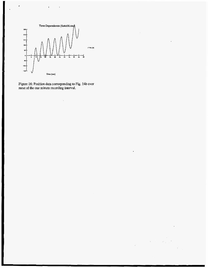
Time Dependence (5x4cO8.csfl

Figure 16: Position data corresponding to Fig. 14b over most of the one minute recording interval.