One-Class Support Measure Machines for Group Anomaly Detection

Krikamol MuandetEmpirical Inference Department

Max Planck Institute for Intelligent SystemsSpemannstraße 38, 72076 Tubingen

Bernhard ScholkopfEmpirical Inference Department

Max Planck Institute for Intelligent SystemsSpemannstraße 38, 72076 Tubingen

Abstract

We propose one-class support measure ma-chines (OCSMMs) for group anomaly detec-tion. Unlike traditional anomaly detection,OCSMMs aim at recognizing anomalous ag-gregate behaviors of data points. The OC-SMMs generalize well-known one-class sup-port vector machines (OCSVMs) to a spaceof probability measures. By formulating theproblem as quantile estimation on distribu-tions, we can establish interesting connec-tions to the OCSVMs and variable kerneldensity estimators (VKDEs) over the inputspace on which the distributions are defined,bridging the gap between large-margin meth-ods and kernel density estimators. In partic-ular, we show that various types of VKDEscan be considered as solutions to a class ofregularization problems studied in this pa-per. Experiments on Sloan Digital Sky Sur-vey dataset and High Energy Particle Physicsdataset demonstrate the benefits of the pro-posed framework in real-world applications.

1 Introduction

Anomaly detection is one of the most important toolsin all data-driven scientific disciplines. Data that donot conform to the expected behaviors often bear someinteresting characteristics and can help domain expertsbetter understand the problem at hand. However, inthe era of data explosion, the anomaly may appearnot only in the data themselves, but also as a resultof their interactions. The main objective of this paperis to investigate the latter type of anomalies. To beconsistent with the previous works (Poczos et al. 2011,Xiong et al. 2011a;b), we will refer to this problem as agroup anomaly detection, as opposed to a traditionalpoint anomaly detection.

Input s

pace

Dist

ributio

n spac

e

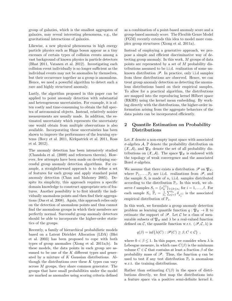
Figure 1: An illustration of two types of group anoma-lies. An anomalous group may be a group of anoma-lous samples which is easy to detect (unfilled points).In this paper, we are interested in detecting anomalousgroups of normal samples (filled points) which is moredifficult to detect because of the higher-order statis-tics. Note that group anomaly we are interested incan only be observed in the space of distributions.

Like traditional point anomaly detection, the groupanomaly detection refers to a problem of finding pat-terns in groups of data that do not conform to expectedbehaviors (Poczos et al. 2011, Xiong et al. 2011a;b).That is, an ultimate goal is to detect interesting ag-gregate behaviors of data points among several groups.In principle, anomalous groups may consist of individ-ually anomalous points, which are relatively easy todetect. On the other hand, anomalous groups of rela-tively normal points, whose behavior as a group is un-usual, is much more difficult to detect. In this work,we are interested in the latter type of group anomalies.Figure 1 illustrates this scenario.

Group anomaly detection may shed light in a widerange of applications. For example, a Sloan Digi-tal Sky Survey (SDSS) has produced a tremendousamount of astronomical data. It is therefore very cru-cial to detect rare objects such as stars, galaxies, orquasars that might lead to a scientific discovery. Inaddition to individual celestial objects, investigatinggroups of them may help astronomers understand theuniverse on larger scales. For instance, the anomalous

group of galaxies, which is the smallest aggregates ofgalaxies, may reveal interesting phenomena, e.g., thegravitational interactions of galaxies.

Likewise, a new physical phenomena in high energyparticle physics such as Higgs boson appear as a tinyexcesses of certain types of collision events among avast background of known physics in particle detectors(Bhat 2011, Vatanen et al. 2012). Investigating eachcollision event individually is no longer sufficient as theindividual events may not be anomalies by themselves,but their occurrence together as a group is anomalous.Hence, we need a powerful algorithm to detect such arare and highly structured anomaly.

Lastly, the algorithm proposed in this paper can beapplied to point anomaly detection with substantialand heterogeneous uncertainties. For example, it is of-ten costly and time-consuming to obtain the full spec-tra of astronomical objects. Instead, relatively noisiermeasurements are usually made. In addition, the es-timated uncertainty which represents the uncertaintyone would obtain from multiple observations is alsoavailable. Incorporating these uncertainties has beenshown to improve the performance of the learning sys-tems (Bovy et al. 2011, Kirkpatrick et al. 2011, Rosset al. 2012).

The anomaly detection has been intensively studied(Chandola et al. (2009) and references therein). How-ever, few attempts have been made on developing suc-cessful group anomaly detection algorithms. For ex-ample, a straightforward approach is to define a setof features for each group and apply standard pointanomaly detection (Chan and Mahoney 2005). De-spite its simplicity, this approach requires a specificdomain knowledge to construct appropriate sets of fea-tures. Another possibility is to first identify the indi-vidually anomalous points and then find their aggrega-tions (Das et al. 2008). Again, this approach relies onlyon the detection of anomalous points and thus cannotfind the anomalous groups in which their members areperfectly normal. Successful group anomaly detectorsshould be able to incorporate the higher-order statis-tics of the groups.

Recently, a family of hierarchical probabilistic modelsbased on a Latent Dirichlet Allocation (LDA) (Bleiet al. 2003) has been proposed to cope with bothtypes of group anomalies (Xiong et al. 2011a;b). Inthese models, the data points in each group are as-sumed to be one of the K different types and gener-ated by a mixture of K Gaussian distributions. Al-though the distributions over these K types can varyacross M groups, they share common generator. Thegroups that have small probabilities under the modelare marked as anomalies using scoring criteria defined

as a combination of a point-based anomaly score and agroup-based anomaly score. The Flexible Genre Model(FGM) recently extends this idea to model more com-plex group structures (Xiong et al. 2011a).

Instead of employing a generative approach, we pro-pose a simple and efficient discriminative way of de-tecting group anomaly. In this work, M groups of datapoints are represented by a set of M probability dis-tributions assumed to be i.i.d. realization of some un-known distribution P. In practice, only i.i.d samplesfrom these distributions are observed. Hence, we cantreat group anomaly detection as detecting the anoma-lous distributions based on their empirical samples.To allow for a practical algorithm, the distributionsare mapped into the reproducing kernel Hilbert space(RKHS) using the kernel mean embedding. By work-ing directly with the distributions, the higher-order in-formation arising from the aggregate behaviors of thedata points can be incorporated efficiently.

2 Quantile Estimation on ProbabilityDistributions

Let X denote a non-empty input space with associatedσ-algebra A, P denote the probability distribution on(X ,A), and PX denote the set of all probability dis-tributions on (X ,A). The space PX is endowed withthe topology of weak convergence and the associatedBorel σ-algebra.

We assume that there exists a distribution P on PX ,where P1, . . . ,P` are i.i.d. realizations from P, andthe sample Si is made of ni i.i.d. samples distributedaccording to the distribution Pi. In this work, we ob-

serve ` samples Si = {x(i)k }1≤k≤ni for i = 1, . . . , `. For

each sample Si, Pi = 1ni

∑nij=1 δx(i)

jis the associated

empirical distribution of Pi.

In this work, we formulate a group anomaly detectionproblem as learning quantile function q : PX → R toestimate the support of P. Let C be a class of mea-surable subsets of PX and λ be a real-valued functiondefined on C, the quantile function w.r.t. (P, C, λ) is

q(β) = inf{λ(C) : P(C) ≥ β,C ∈ C} ,

where 0 < β ≤ 1. In this paper, we consider when λ isLebesgue measure, in which case C(β) is the minimumvolume C ∈ C that contains at least a fraction β of theprobability mass of P. Thus, the function q can beused to test if any test distribution Pt is anomalousw.r.t. the training distributions.

Rather than estimating C(β) in the space of distri-butions directly, we first map the distributions intoa feature space via a positive semi-definite kernel k.

Our class C is then implicitly defined as the set ofhalf-spaces in the feature space. Specifically, Cw ={P | fw(P) ≥ ρ} where (w, ρ) are respectively a weightvector and an offset parametrizing a hyperplane in thefeature space associated with the kernel k. The op-timal (w, ρ) is obtained by minimizing a regularizerwhich controls the smoothness of the estimated func-tion describing C.

3 One-Class Support MeasureMachines

In order to work with the probability distributions ef-ficiently, we represent the distributions as mean func-tions in a reproducing kernel Hilbert space (RKHS)(Berlinet and Agnan 2004, Smola et al. 2007). For-mally, let H denote an RKHS of functions f : X → Rwith reproducing kernel k : X × X → R. The kernelmean map from PX into H is defined as

µ : PX → H, P 7−→∫Xk(x, ·) dP(x) . (1)

We assume that k(x, ·) is bounded for any x ∈ X . Forany P, letting µP = µ(P), one can show that EP[f ] =〈µP, f〉H, for all f ∈ H.

The following theorem due to Fukumizu et al. (2004)and Sriperumbudur et al. (2010) gives a promisingproperty of representing distributions as mean ele-ments in the RKHS.

Theorem 1. The kernel k is characteristic if and onlyif the map (1) is injective.

Examples of characteristic kernels include GaussianRBF kernel and Laplace kernel. Using the character-istic kernel k, Theorem 1 implies that the map (1) pre-serves all information about the distributions. Hence,one can apply many existing kernel-based learning al-gorithms to the distributions as if they are individualsamples with no information loss.

Intuitively, one may view the mean embeddings of thedistributions as their feature representations. Thus,our approach is in line with previous attempts in groupanomaly detection that find a set of appropriate fea-tures for each group. On the one hand, however, themean embedding approach captures all necessary in-formation about the groups without relying heavilyon a specific domain knowledge. On the other hand, itis flexible to choose the feature representation that issuitable to the problem at hand via the choice of thekernel k.

3.1 OCSMM Formulation

Using the mean embedding representation (1), the pri-mal optimization problem for one-class SMM can be

subsequently formulated in an analogous way to theone-class SVM (Scholkopf et al. 2001) as follow:

minimizew,b,ξ,ρ

1

2〈w,w〉H − ρ+

1

ν`

∑i=1

ξi (2a)

subject to 〈w, µPi〉H ≥ ρ− ξi, ξi ≥ 0 (2b)

where ξi denote slack variables and ν ∈ (0, 1] is a trade-off parameter corresponding to an expected fraction ofoutliers within the feature space. The trade-off ν isan upper bound on the fraction of outliers and lowerbound on the fraction of support measures (Scholkopfet al. 2001).

The trade-off parameter ν plays an important role ingroup anomaly detection. Small ν implies that anoma-lous groups are rare compared to the normal groups.Too small ν leads to some anomalous groups being re-jected. On the other hand, large ν implies that anoma-lous groups are common. Too large ν leads to somenormal groups being accepted as anomaly. As groupanomaly is subtle, one need to choose ν very carefullyto reduce the effort in the interpretation of the results.

By introducing Lagrange multipliers α, we have w =∑`i=1 αiµPi =

∑`i=1 αiEPi [k(x, ·)] and the dual form of

(2) can be written as

minimizeα

1

2

∑i=1

∑j=1

αiαj〈µPi , µPj 〉H (3a)

subject to 0 ≤ αi ≤1

ν`,∑i=1

αi = 1 . (3b)

Note that the dual form is a quadratic programmingand depends on the inner product 〈µPi , µPj 〉H. Giventhat we can compute 〈µPi , µPj 〉H, we can employ thestandard QP solvers to solve (3).

3.2 Kernels on Probability Distributions

From (3), we can see that µP is a feature map asso-ciated with the kernel K : PX × PX → R, definedas K(Pi,Pj) = 〈µPi , µPj 〉H. It follows from Fubini’stheorem and reproducing property of H that

〈µPi , µPj 〉H =

∫∫〈k(x, ·), k(y, ·)〉H dPi(x) dPj(y)

=

∫∫k(x, y) dPi(x) dPj(y) . (4)

Hence, K is a positive definite kernel on PX . Giventhe sample sets S1, . . . , S`, one can estimate (4) by

K(Pi, Pj) =1

ni · nj

ni∑k=1

nj∑l=1

k(x(i)k , x

(j)l ) (5)

where x(i)k ∈ Si, x

(j)l ∈ Sj , and ni is the number of

samples in Si for i = 1, . . . , `.

Previous works in kernel-based anomaly detectionhave shown that the Gaussian RBF kernel is moresuitable than some other kernels such as polynomialkernels (Hoffmann 2007). Thus we will focus primar-ily on the Gaussian RBF kernel given by

kσ(x, x′) = exp

(−‖x− x

′‖22σ2

), x, x′ ∈ X (6)

where σ > 0 is a bandwidth parameter. In the sequel,we denote the reproducing kernel Hilbert space asso-ciated with kernel kσ by Hσ. Also, let Φ : X → Hσ bea feature map such that kσ(x, x′) = 〈Φ(x),Φ(x′)〉Hσ .

In group anomaly detection, we always observe thei.i.d. samples from the distribution underlying thegroup. Thus, it is natural to use the empirical ker-nel (5). However, one may relax this assumption andapply the kernel (4) directly. For instance, if we have aGaussian distribution Pi = N (mi,Σi) and a GaussianRBF kernel kσ, we can compute the kernel analyticallyby

K(Pi,Pj) =exp

(− 1

2 (mi −mj)TB−1(mi −mj)

)| 1σ2 Σi + 1

σ2 Σj + I| 12(7)

where B = Σi + Σj + σ2I. This kernel is particularlyuseful when one want to incorporate the point-wise un-certainty of the observation into the learning algorithm(Muandet et al. 2012). More details will be given inSection 4.2 and 5).

4 Theoretical Analysis

This section presents some theoretical analyses. Thegeometrical interpretation of OCSMMs is given in Sec-tion 4.1. Then, we discuss the connection of OCSMMto the kernel density estimator in Section 4.2. In thesequel, we will focus on the translation-invariant kernelfunction to simplify the analysis.

4.1 Geometric Interpretation

For translation-invariant kernel, k(x, x) is constant forall x ∈ X . That is, ‖Φ(x)‖H = τ for some constantρ. This implies that all of the images Φ(x) lie on thesphere in the feature space (cf. Figure 2a). Conse-quently, the following inequality holds

‖µP‖H =

∥∥∥∥∫ k(x, ·) dP(x)

∥∥∥∥H≤∫‖k(x, ·)‖H dP(x) = τ ,

which shows that all mean embeddings lie inside thesphere (cf. Figure 2a). As a result, we can establishthe existence and uniqueness of the separating hyper-plane w in (2) through the following theorem.

Theorem 2. There exists a unique separating hy-perplane w as a solution to (2) that separatesµP1

, µP2, . . . , µP` from the origin.

Proof. Due to the separability of the feature mapsΦ(x), the convex hull of the mean embeddingsµP1

, µP2, . . . , µP` does not contain the origin. The ex-

istence and uniqueness of the hyperplane then followsfrom the supporting hyperplane theorem (Scholkopfand Smola 2001). �

By Theorem 2, the OCSMM is a simple generalizationof OCSVM to the space of probability distributions.Furthermore, the straightforward generalization willallow for a direct application of an efficient learningalgorithm as well as existing theoretical results.

There is a well-known connection between the solutionof OCSVM with translation invariant kernels and thecenter of the minimum enclosing sphere (MES) (Taxand Duin 1999; 2004). Intuitively, this is not the casefor OCSMM, even when the kernel k is translation-invariant, as illustrated in Figure 2b. Fortunately, theconnection between OCSMM and MES can be madeprecise by applying the spherical normalization

〈µP, µQ〉H 7−→〈µP, µQ〉H√

〈µP, µP〉H〈µQ, µQ〉H(8)

After the normalization, ‖µP‖H = 1 for all P ∈ PX .That is, all mean embeddings lie on the unit spherein the feature space. Consequently, the OCSMM andMES are equivalent after the normalization.

Given the equivalence between OCSMM and MES, itis natural to ask if the spherical normalization (8) pre-serves the injectivity of the Hilbert space embedding.In other words, is there an information loss after thenormalization? The following theorem answers thisquestion for kernel k that satisfies some reasonable as-sumptions.

Theorem 3. Assume that k is characteristic and thesamples are linearly independent in the feature spaceH. Then, the spherical normalization preserves theinjectivity of the mapping µ : PX → H.

Proof. Let us assume the normalization does not pre-serve the injectivity of the mapping. Thus, there ex-ist two distinct probability distributions P and Q forwhich

µP = µQ∫k(x, ·) dP(x) =

∫k(x, ·) dQ(x)∫

k(x, ·) d(P−Q)(x) = 0 .

Origin

Φ(x)

µP = Ex∼P[Φ(x)]

Conv({Φ(x)})

(a) feature map and mean map

Origin

ρ/‖w

‖

ROCSVM

ROCSMM

(b) minimum enclosing sphere

Origin

Conv({Φ(x)})

µP

(c) spherical normalization

Figure 2: (a) The two dimensional representation of the RKHS of Gaussian RBF kernels. Since the kernelsdepend only on x − x′, k(x, x) is constant. Therefore, all feature maps Φ(x) (black dots) lie on a sphere infeature space. Hence, for any probability distribution P, its mean embedding µP always lies in the convex hullof the feature maps, which in this case, forms a segment of the sphere. (b) In general, the solution of OCSMMis different from the minimum enclosing sphere. (c) Three dimensional sphere in the feature space. For theGaussian RBF kernel, the kernel mean embeddings of all distributions always lie inside the segment of thesphere. In addition, the angle between any pair of mean embeddings is always greater than zero. Consequently,the mean embeddings can be scaled, e.g., to lie on the sphere, and the map is still injective.

As P 6= Q, the last equality holds if and only if thereexists x ∈ X for which k(x, ·) are linearly dependent,which contradicts the assumption. Consequently, thespherical normalization must preserve the injectivityof the mapping. �

The Gaussian RBF kernel satisfies the assumptiongiven in Theorem 3 as the kernel matrix will be full-rank and thereby the samples are linearly independentin the feature space. Figure 2c depicts an effect of thespherical normalization.

It is important to note that the spherical normalizationdoes not necessarily improve the performance of theOCSMM. It ensures that all the information about thedistributions are preserved.

4.2 OCSMM and Density Estimation

In this section we make a connection between the OC-SMM and kernel density estimation (KDE). First, wegive a definition of the KDE. Let x1, x2, . . . , xn be ani.i.d. samples from some distribution F with unknowndensity f , the KDE of f is defined as

f(y) =1

nh

n∑i=1

k

(y − xih

)(9)

For f to be a density, we require that the kernel satis-fies k(·, ·) ≥ 0 and

∫k(x, ·) dx = 1, which includes, for

example, the Gaussian kernel, the multivariate Stu-dent kernel, and the Laplacian kernel.

When ν = 1, it is well-known that, under some techni-cal assumptions, the OCSVM corresponds exactly tothe KDE (Scholkopf et al. 2001). That is, the solution

w of (2) can be written as a uniform sum over trainingsamples similar to (9). Moreover, setting ν < 1 yieldsa sparse representation where the summand consistsof only support vectors of the OCSVM.

Interestingly, we can make a similar correspondencebetween the KDE and the OCSMM. It follows fromLemma 4 of Muandet et al. (2012) that for cer-tain classes of training probability distributions, theOCSMM on these distributions corresponds to theOCSVM on some training samples equipped withan appropriate kernel function. To understand thisconnection, consider the OCSMM with the GaussianRBF kernel kσ and isotropic Gaussian distributionsN (m1;σ2

1),N (m2;σ22), . . . ,N (mn;σ2

n)1. We analyzethis scenario under two conditions:

(C1) Identical bandwidth. If σi = σj for all 1 ≤i, j ≤ n, the OCSMM is equivalent to the OCSVMon the training samples m1,m2, . . . ,mn with GaussianRBF kernel kσ2+σ2

i(cf. the kernel (7)). Hence, the

OCSMM corresponds to the OCSVM on the means ofthe distributions with kernel of larger bandwidth.

(C2) Variable bandwidth. Similarly, if σi 6= σjfor some 1 ≤ i, j ≤ n, the OCSMM is equivalent tothe OCSVM on the training samples m1,m2, . . . ,mn

with Gaussian RBF kernel kσ2+σ2i. Note that the ker-

nel bandwidth may be different at each training sam-ples. Thus, OCSMM in this case corresponds to theOCSVM with variable bandwidth parameters.

1We adopt the Gaussian distributions here for the sakeof simplicity. More general statement for non-Gaussiandistributions follows straightforwardly.

On the one hand, the above scenario allows theOCSVM to cope with noisy/uncertain inputs, lead-ing to more robust point anomaly detection algorithm.That is, we can treat the means as the measurementsand the covariances as the measurement uncertainties(cf. Section 5.2). On the other hand, one can alsointerpret the OCSMM when ν = 1 as a generalizationof traditional KDE, where we have a data-dependentbandwidth at each data point. This type of KDE isknown in the statistics as variable kernel density es-timators (VKDEs) (Abramson 1982, Breiman et al.1977, Terrell and Scott 1992). For ν < 1, the OC-SMM gives a sparse representation of the VKDE.

Formally, the VKDE is characterized by (9) with anadaptive bandwidth h(xi). For example, the band-width is adapted to be larger where the data are lessdense, with the aim to reduce the bias. There are basi-cally two different views of VKDE. The first is knownas a balloon estimator (Terrell and Scott 1992). Essen-tially, its bandwidth may depend only on the point atwhich the estimate is taken, i.e., the bandwidth in (9)may be written as h(y). The second type of VKDE is asample smoothing estimator (Terrell and Scott 1992).As opposed to the balloon estimator, it is a mixtureof individually scaled kernels centered at each obser-vation, i.e., the bandwidth is h(xi). The advantageof balloon estimator is that it has a straightforwardasymptotic analysis, but the final estimator may notbe a density. The sample smoothing estimator is adensity if k is a density, but exhibits non-locality.

Both types of the VKDEs may be seen from the OC-SMM point of view. Firstly, under the condition (C1),the balloon estimator can be recovered by consider-ing different test distribution Pt = N (mt;σt). Asσt → 0, one obtain the standard KDE on mt. Sim-ilarly, the OCSMM under the condition (C2) withPt = δmt gives the sample smoothing estimator. Inter-estingly, the OCSMM under the condition (C2) withPt = N (mt;σt) results in a combination of these twotypes of the VKDEs.

In summary, we show that many variants of KDE canbe seen as solutions to the regularization functional(2), and thereby provides an insight into a connectionbetween large-margin approach and kernel density es-timation.

5 Experiments

We firstly illustrate a fundamental difference be-tween point and group anomaly detection problems.Then, we demonstrate an advantage of OCSMM onuncertain data when the noise is observed explic-itly. Lastly, we compare the OCSMM with ex-isting group anomaly detection techniques, namely,

K-nearest neighbor (KNN) based anomaly detection(Zhao and Saligrama 2009) with NP-L2 divergence andNP-Renyi divergence (Poczos et al. 2011), and Multi-nomial Genre Model (MGM) (Xiong et al. 2011b) onSloan Digital Sky Survey (SDSS) dataset and HighEnergy Particle Physics dataset.

Model Selection and Setup. One of the long-standing problems of one-class algorithms is modelselection. Since no labeled data is available duringtraining, we cannot perform cross validation. To en-courage a fair comparison of different algorithms inour experiments, we will try out different parame-ter settings and report the best performance of eachalgorithm. We believe this simple approach shouldserve its purpose at reflecting the relative performanceof different algorithms. We will employ the Gaus-sian RBF kernel (6) throughout the experiments. Forthe OCSVM and the OCSMM, the bandwidth pa-

rameter σ2 is fixed at median{‖x(i)k − x(j)l ‖2} for all

i, j, k, l where x(i)k denotes the k-th data point in the

i-th group, and we consider ν = (0.1, 0.2, . . . , 0.9).The OCSVM treats group means as training sam-ples. For synthetic experiments with OCSMM, we usethe empirical kernel (5), whereas the non-linear kernelK(Pi,Pj) = exp(‖µPi − µPj‖2H/2γ2) will be used forreal data where we set γ = σ. Our experiments sug-gest that these choices of parameters usually work wellin practice. For KNN-L2 and KNN-Renyi (α=0.99),we consider when there are 3,5,7,9, and 11 nearestneighbors. For MGM, we follow the same experimen-tal setup as in Xiong et al. (2011b).

5.1 Synthetic Data

To illustrate the difference between point anomalyand group anomaly, we represent the group of datapoints by the 2-dimensional Gaussian distribution. Wegenerate 20 normal groups with the covariance Σ =[0.01, 0.008; 0.008, 0.01]. The means of these groupsare drawn uniformly from [0, 1]. Then, we generate 2anomalous groups of Gaussian distributions whose co-variances are rotated by 60 degree from the covarianceΣ. Furthermore, we perturb one of the normal groupsto make it relatively far from the rest of the datasetto introduce an additional degree of anomaly (cf. Fig-ure 3a). Lastly, we generate 100 samples from each ofthese distributions to form the training set.

For the OCSVM, we represent each group by its empir-ical average. Since the expected proportion of outliersin the dataset is approximately 10%, we use ν = 0.1accordingly for both OCSVM and OCSMM. Figure 3adepicts the result which demonstrates that the OC-SMM can detect anomalous aggregate patterns unde-tected by the OCSVM.

One-Class Support Vector Machine

One-Class Support Measure Machine

(a) OCSVM vs OCSMM (b) The results of the OCSMM on the mixture of Gaussian dataset

Figure 3: (a) The results of group anomaly detection on synthetic data obtained from the OCSVM and theOCSMM. Blue dashed ovals represent the normal groups, whereas red ovals represent the detected anomalousgroups. The OCSVM is only able to detect the anomalous groups that are spatially far from the rest in thedataset, whereas the OCSMM also takes into account other higher-order statistics and therefore can also detectanomalous groups which possess distinctive properties. (b) The results of the OCSMM on the synthetic data ofthe mixture of Gaussian. The shaded boxes represent the anomalous groups that have different mixing proportionto the rest of the dataset. The OCSMM is able to detects the anomalous groups although they look reasonablynormal and cannot be easily distinguished from other groups in the data set based only on an inspection.

Then, we conduct similar experiment as that in Xionget al. (2011b). That is, the groups are representedas a mixture of four 2-dimensional Gaussian distri-butions. The means of the mixture components are[−1,−1], [1,−1], [0, 1], [1, 1] and the covariances areall Σ = 0.15 × I2, where I2 denotes the 2D iden-tity matrix. Then, we design two types of normalgroups, which are specified by two mixing propor-tions [0.22, 0.64, 0.03, 0.11] and [0.22, 0.03, 0.64, 0.11],respectively. To generate a normal group, we first de-cide with probability [0.48, 0.52] which mixing propor-tion will be used. Then, the data points are generatedfrom mixture of Gaussian using the specified mixingproportion. The mixing proportion of the anomalousgroup is [0.61, 0.1, 0.06, 0.23].

We generated 47 normal groups with ni ∼Poisson(300) instances in each group. Note that theindividual samples in each group are perfectly normalcompared to other samples. To test the performanceof our technique, we inject the group anomalies, wherethe individual points are normal, but they together asa group look anomalous. In this anomalous group theindividual points are samples from one of the K = 4normal topics, but the mixing proportion was differentfrom both of the normal mixing proportions. We inject3 anomalous groups into the data set. The OCSMMis trained using the same setting as in the previousexperiment. The results are depicted in Figure 3b.

5.2 Noisy Data

As discussed at the end of Section 3.2, the OCSMMmay be adopted to learn from data points whose un-certainties are observed explicitly. To illustrate thisclaim, we generate samples from the unit circle usingx = cos θ + ε and y = sin θ + ε where θ ∼ (−π, π] andε is a zero-mean isotropic Gaussian noise N (0, 0.05).A different point-wise Gaussian noise N (0, ωi) whereωi ∈ (0.2, 0.3) is further added to each point to simu-late the random measurement corruption. In this ex-periment, we assume that ωi is available during train-ing. This situation is often encountered in many ap-plications such as astronomy and computational biol-ogy. Both OCSVM and OCSMM are trained on thecorrupted data. As opposed to the OCSVM that con-siders only the observed data points, the OCSMM alsouses ωi for every point via the kernel (7). Then, weconsider a slightly more complicate data generated byx = r · cos(θ) and y = r · sin(θ) where r = sin(4θ) + 2and θ ∈ (0, 2π]. The data used in both examples areillustrated in Figure 4.

As illustrated by Figure 4, the density function es-timated by the OCSMM is relatively less susceptibleto the additional corruption than that estimated bythe OCSVM, and tends to estimate the true densitymore accurately. This is not surprising because we alsotake into account an additional information about theuncertainty. However, this experiment suggests thatwhen dealing with uncertain data, it might be ben-

uncorrupted data corrupted data one−class SVM one−class SMM

uncorrupted data corrupted data one−class SVM one−class SMM

Figure 4: The density functions estimated by theOCSVM and the OCSMM using the corrupted data.

eficial to also estimate the uncertainty, as commonlyperformed in astronomy, and incorporate it into themodel. This scenario has not been fully investigatedin AI and machine learning communities. Our frame-work provides one possible way to deal with such ascenario.

5.3 Sloan Digital Sky Survey

Sloan Digital Sky Survey (SDSS)2 consists of a series ofmassive spectroscopic surveys of the distant universe,the milky way galaxies, and extrasolar planetary sys-tems. The SDSS datasets contain images and spectraof more than 930,000 galaxies and more than 120,000quasars.

In this experiment, we are interested in identifyinganomalous groups of galaxies, as previously studiedin Poczos et al. (2011) and Xiong et al. (2011a;b). Toreplicate the experiments conducted in Xiong et al.(2011b), we use the same dataset which consists of505 spatial clusters of galaxies. Each of which con-tains about 10-15 galaxies. The data were prepro-cessed by PCA to reduce the 1000-dimensional featuresto 4-dimensional vectors.

To evaluate the performance of different algorithms todetect group anomaly, we consider artificially randominjections. Each anomalous group is constructed byrandomly selecting galaxies. There are 50 anomalousgroups of galaxies in total. Note that although thesegroups of galaxies contain usual galaxies, their aggre-gations are anomalous due to the way the groups areconstructed.

The average precision (AP) and area under the ROCcurve (AUC) from 10 random repetitions are shown inFigure 5. Based on the average precision, KNN-L2,MGM, and OCSMM achieve similar results on thisdataset and KNN-Renyi outperforms all other algo-rithms. On the other hand, the OCSMM and KNN-

2See http://www.sdss.org for the detail of the surveys.

KNN−L2 KNN−Renyi MGM OCSVM OCSMM

0.1

0.15

0.2

0.25

0.3

0.35

0.4

0.45

0.5

Avera

ge P

recis

ion

KNN−L2 KNN−Renyi MGM OCSVM OCSMM

0.45

0.5

0.55

0.6

0.65

0.7

0.75

0.8

AU

C

Figure 5: The average precision (AP) and area un-der the ROC curve (AUC) of different group anomalydetection algorithms on the SDSS dataset.

Renyi achieve highest AUC scores on this dataset.Moreover, it is clear that point anomaly detection us-ing the OCSVM fails to detect group anomalies.

5.4 High Energy Particle Physics

In this section, we demonstrate our group anomalydetection algorithm in high energy particle physics,which is largely the study of fundamental parti-cles, e.g., neutrinos, and their interactions. Essen-tially, all particles and their dynamics can be de-scribed by a quantum field theory called the Stan-dard Model. Hence, given massive datasets from high-energy physics experiments, one is interested in discov-ering deviations from known Standard Model physics.

Searching for the Higgs boson, for example, has re-cently received much attention in particle physics andmachine learning communities (see e.g., Bhat (2011),Vatanen et al. (2012) and references therein). A newphysical phenomena usually manifest themselves astiny excesses of certain types of collision events amonga vast background of known physics in particle detec-tors.

Anomalies occur as a cluster among the backgrounddata. The background data distribution contaminatedby these anomalies will therefore be different from thetrue background distribution. It is very difficult to de-tect this difference in general because the contamina-tion can be considerably small. In this experiment, weconsider similar condition as in Vatanen et al. (2012)and generate data using the standard HEP MonteCarlo generators such as PYTHIA3. In particular, weconsider a Monte Carlo simulated events where theHiggs is produced in association with the W bosonand decays into two bottom quarks.

The data vector consists of 5 variables (px, py, pz, e,m)corresponding to different characteristics of the topol-ogy of a collision event. The variables px, py, pz, e rep-

3http://home.thep.lu.se/∼torbjorn/Pythia.html

0 0.25 0.5 0.75 10

0.25

0.5

0.75

1

false positive

tru

e p

ositiv

emH = 100GeV

KNN−L2

KNN−Renyi

MGM

OCSVM

OCSMM

0 0.25 0.5 0.75 10

0.25

0.5

0.75

1

false positive

tru

e p

ositiv

e

mH = 115GeV

KNN−L2

KNN−Renyi

MGM

OCSVM

OCSMM

0 0.25 0.5 0.75 10

0.25

0.5

0.75

1

false positive

tru

e p

ositiv

e

mH = 135GeV

KNN−L2

KNN−Renyi

MGM

OCSVM

OCSMM

0 0.25 0.5 0.75 10

0.25

0.5

0.75

1

false positive

tru

e p

ositiv

e

mH = 150GeV

KNN−L2

KNN−Renyi

MGM

OCSVM

OCSMM

Figure 6: The ROC of different group anomaly detection algorithms on the Higgs boson datasets withvarious Higgs masses mH . The associated AUC scores for different settings, sorted in the same or-der appeared in the figure, are (0.6835,0.6655,0.6350,0.5125,0.7085), (0.5645,0.6783,0.5860,0.5263,0.7305),(0.8190,0.7925,0.7630,0.4958,0.7950), and (0.6713,0.6027,0.6165,0.5862,0.7200).

resents the momentum four-vector in units of GeVwith c = 1. The variable m is the particle mass in thesame unit. The signal looks slightly different for dif-ferent Higgs masses mH , which is an unknown free pa-rameter in the Standard Model. In this experiment, weconsider mH = 100, 115, 135, and 150 GeV. We gener-ate 120 groups of collision events, 100 of which containonly background signals, whereas the rest also containthe Higgs boson collision events. For each group, thenumber of observable particles ranges from 200 to 500particles. The goal is to detect the anomalous groupsof signals which might contain the Higgs boson with-out prior knowledge of mH .

Figure 6 depicts the ROC of different group anomalydetection algorithms. The OCSMM and KNN-basedgroup anomaly detection algorithms tend to achievecompetitive performance and outperform the MGMalgorithm. Moreover, it is clear that traditional pointanomaly detection algorithm fails to detect high-levelanomalous structures.

6 Conclusions and Discussions

To conclude, we propose a simple and efficient algo-rithm for detecting group anomalies called one-classsupport measure machine (OCSMM). To handle ag-gregate behaviors of data points, groups are repre-sented as probability distributions which account forhigher-order information arising from those behaviors.The set of distributions are represented as mean func-tions in the RKHS via the kernel mean embedding. Wealso extend the relationship between the OCSVM andthe KDE to the OCSMM in the context of variablekernel density estimation, bridging the gap betweenlarge-margin approach and kernel density estimation.We demonstrate the proposed algorithm on both syn-thetic and real-world datasets, which achieve compet-itive results compared to existing group anomaly de-

tection techniques.

It is vital to note the differences between the OCSMMand hierarchical probabilistic models such as MGMand FGM. Firstly, the probabilistic models assumethat data are generated according to some paramet-ric distributions, i.e., mixture of Gaussian, whereasthe OCSMM is nonparametric in the sense that noassumption is made about the distributions. It istherefore applicable to a wider range of applications.Secondly, the probabilistic models follow a bottom-up approach. That is, detecting group-based anoma-lies requires point-based anomaly detection. Thus,the performance also depends on how well anomalouspoints can be detected. Furthermore, it is computa-tional expensive and may not be suitable for large-scale datasets. On the other hand, the OCSMMadopts the top-down approach by detecting the group-based anomalies directly. If one is interested in find-ing anomalous points, this can be done subsequentlyin a group-wise manner. As a result, the top-downapproach is generally less computational expensiveand can be used efficiently for online applications andlarge-scale datasets.

References

I. S. Abramson. On bandwidth variation in kernelestimates-a square root law. The Annals of Statistics,10(4):1217–1223, 1982.

A. Berlinet and T. C. Agnan. Reproducing Kernel HilbertSpaces in Probability and Statistics. Kluwer AcademicPublishers, 2004.

P. C. Bhat. Multivariate Analysis Methods in ParticlePhysics. Ann.Rev.Nucl.Part.Sci., 61:281–309, 2011.

D. M. Blei, A. Y. Ng, and M. I. Jordan. Latent dirichletallocation. Journal of Machine Learning Research, 3:993–1022, 2003.

J. Bovy, J. F. Hennawi, D. W. Hogg, A. D. Myers, J. A.Kirkpatrick, D. J.Schlegel, N. P. Ross, E. S. Sheldon,

I. D. McGreer, D. P. Schneider, and B. A. Weaver. Thinkoutside the color box: Probabilistic target selection andthe sdss-xdqso quasar targeting catalog. The Astrophys-ical Journal, 729(2):141, 2011.

L. Breiman, W. Meisel, and E. Purcell. Variable kernelestimates of multivariate densities. Technometrics, 19(2):135–144, 1977.

P. K. Chan and M. V. Mahoney. Modeling multipletime series for anomaly detection. In Proceedings ofthe 5th IEEE International Conference on Data Mining(ICDM), pages 90–97. IEEE Computer Society, 2005.

V. Chandola, A. Banerjee, and V. Kumar. Anomaly detec-tion: A survey. ACM Comput. Surv., 41(3):1–58, July2009.

K. Das, J. Schneider, and D. B. Neill. Anomaly pattern de-tection in categorical datasets. In ACM-SIGKDD, pages169–176. ACM, 2008.

K. Fukumizu, F. R. Bach, and M. I. Jordan. Dimension-ality reduction for supervised learning with reproducingkernel hilbert spaces. Journal of Machine Learning Re-search, 5:73–99, December 2004.

H. Hoffmann. Kernel PCA for novelty detection. PatternRecognition, 40(3):863–874, 2007.

J. A. Kirkpatrick, D. J. Schlegel, N. P. Ross, A. D. Myers,J. F. Hennawi, E. S.Sheldon, D. P. Schneider, and B. A.Weaver. A simple likelihood method for quasar targetselection. The Astrophysical Journal, 743(2):125, 2011.

K. Muandet, K. Fukumizu, F. Dinuzzo, and B. Scholkopf.Learning from distributions via support measure ma-chines. In Advances in Neural Information ProcessingSystems (NIPS), pages 10–18. 2012.

B. Poczos, L. Xiong, and J. G. Schneider. Nonpara-metric divergence estimation with applications to ma-chine learning on distributions. In Proceedings of the27th Conference on Uncertainty in Artificial Intelligence(UAI), pages 599–608, 2011.

N. P. Ross, A. D. Myers, E. S. Sheldon, C. Yche, M. A.Strauss, J. Bovy, J. A. Kirkpatrick, G. T. Richards,ric Aubourg, M. R. Blanton, W. N. Brandt, W. C.Carithers, R. A. C. Croft, R. da Silva, K. Dawson,D. J. Eisenstein, J. F. Hennawi, S. Ho, D. W. Hogg,K.-G. Lee, B. Lundgren, R. G. McMahon, J. Miralda-Escud, N. Palanque-Delabrouille, I. Pris, P. Petitjean,M. M. Pieri, J. Rich, N. A. Roe, D. Schiminovich, D. J.Schlegel, D. P. Schneider, A. Slosar, N. Suzuki, J. L.Tinker, D. H. Weinberg, A. Weyant, M. White, andW. M. Wood-Vasey. The sdss-iii baryon oscillation spec-troscopic survey: Quasar target selection for data releasenine. The Astrophysical Journal Supplement Series, 199(1):3, 2012.

B. Scholkopf and A. J. Smola. Learning with Kernels:Support Vector Machines, Regularization, Optimization,and Beyond. MIT Press, Cambridge, MA, USA, 2001.ISBN 0262194759.

B. Scholkopf, J. C. Platt, J. C. Shawe-Taylor, A. J. Smola,and R. C. Williamson. Estimating the support of a high-dimensional distribution. Neural Computation, 13:1443–1471, 2001.

A. Smola, A. Gretton, L. Song, and B. Scholkopf. A hilbertspace embedding for distributions. In Proceedings of the18th International Conference on Algorithmic LearningTheory, pages 13–31. Springer-Verlag, 2007.

B. K. Sriperumbudur, A. Gretton, K. Fukumizu,B. Scholkopf, and G. R. G. Lanckriet. Hilbert space em-beddings and metrics on probability measures. Journalof Machine Learning Research, 2010.

D. M. J. Tax and R. P. W. Duin. Support vector domaindescription. Pattern Recognition Letters, 20:1191–1199,1999.

D. M. J. Tax and R. P. W. Duin. Support vector datadescription. Machine Learning, 54(1):45–66, 2004.

G. R. Terrell and D. W. Scott. Variable kernel densityestimation. The Annals of Statistics, 20(3):1236–1265,1992.

T. Vatanen, M. Kuusela, E. Malmi, T. Raiko, T. Aaltonen,and Y. Nagai. Semi-supervised detection of collectiveanomalies with an application in high energy particlephysics. In IJCNN, pages 1–8. IEEE, 2012.

L. Xiong, B. Poczos, and J. Schneider. Group anomalydetection using flexible genre models. In Proceedingsof Advances in Neural Information Processing Systems(NIPS), 2011a.

L. Xiong, B. Poczos, J. G. Schneider, A. Connolly, andJ. VanderPlas. Hierarchical probabilistic models forgroup anomaly detection. Journal of Machine LearningResearch - Proceedings Track, 15:789–797, 2011b.

M. Zhao and V. Saligrama. Anomaly detection with scorefunctions based on nearest neighbor graphs. In Pro-ceedings of Advances in Neural Information ProcessingSystems (NIPS), pages 2250–2258, 2009.