A COMPUTATIONAL SIMULATION OF HEAT TRANSFER TO TURBULENT FLOW SEPARATION USING NANO FLUID IN A

CONCENTRIC PIPE

OON CHEEN SEAN

DISSERTATION SUBMITTED IN FULFILMENT OF THE REQUIREMENTS FOR THE DEGREE OF MASTER OF

ENGINEERING SCIENCE

FACULTY OF ENGINEERING UNIVERSITY OF MALAYA

KUALA LUMPUR

2013

ii

UNIVERSITI MALAYA

ORIGINAL LITERARY WORK DECLARATION

Name of Candidate: OON CHEEN SEAN

Registration/Matric No: KGA 100039

Name of Degree: MASTER OF ENGINEERING SCIENCE

Title: A COMPUTATIONAL SIMULATION OF HEAT TRANSFER TO TURBULENT

FLOW SEPARATION USING NANO FLUID IN A CONCENTRIC PIPE

Field of Study: HEAT TRANSFER

I do solemnly and sincerely declare that: (1) I am the sole author/writer of this Work; (2) This Work is original; (3) Any use of any work in which copyright exists was done by way of fair dealing and for permitted purposes and any excerpt or extract from, or reference to or reproduction of any copyright work has been disclosed expressly and sufficiently and the title of the work and its authorship have been acknowledged in this Work; (4) I do not have any actual knowledge nor do I ought reasonably to know that the making of this work constitutes an infringement of any copyright work; (5) I hereby assign all and every rights in the copyright to this Work to the University of Malaya (“UM”), who henceforth shall be owner of the copyright in this Work and that any reproduction or use in any form or by any means whatsoever is prohibited without the written consent of UM having been first had and obtained; (6) I am fully aware that if in the course of making this Work I have infringed any copyright whether intentionally or otherwise, I may be subject to legal action or any other action as may be determined by UM.

Candidate’s Signature: Date:

Subscribed and solemnly declared before,

Witness’s Signature: Date:

Name:

Designation:

iii

ABSTRACT

Backward facing step play a vital role in the design of many equipment and

engineering applications where heat transfer is concerned. The investigation is mainly

concentrated on turbulent fluid flows in an annular passage utilizing computational fluid

dynamic package (FLUENT). Present research work is complied into two parts. The first

section is planned to gather results of investigation on various numerical model parameters

and compare with the experimental results obtained previously. The results were then

verified by using various techniques such as mesh independent study, surface roughness

study and the effect of various viscous models. The second part of the research was focused

on the numerical simulation of preliminary experimental setup. The numerical simulation

on heat transfer over a considerable number of parameters were carried out; including wall

heat flux, fluid flow velocity, separation step height, different concentrations and various

nanofluids. The increase of flow reduces the surface temperature along the pipe to a

minimum point then gradually increases up to the maximum and hold for the rest of the

pipe. The minimum surface temperature is obtained at flow reattachment point. The

position of the minimum temperature point is dependent on the flow velocity over sudden

expansion. Generally, the local Nusselt number (Nu) increases with the increase of the

Reynolds number. Heat transfer coefficient of nanofluids increases with increase in the

volume concentration of nanofluids and Reynolds number s. Higher temperature operation

of the nanofluids y ields higher percentage increase in heat transfer rate. Finally, with the

advent of computational fluid dynamic software, a fair and agreeable results were obtained

for the present research.

iv

ABSTRAK

Aliran ke belakang menghadap tetanga memainkan peranan yang penting dalam

reka bentuk peralatan dan aplikasi kejuruteraan yang berkaitan dengan pemindahan haba.

Penyelidikan ini tertumpu pada cecair aliran gelora di dalam saluran anulus menggunakan

pakej dinamik bendalir pengiraan (FLUENT). Kerja-kerja penyelidikan dibahagikan

kepada dua bahagian. Seksyen pertama dirancang untuk mengumpul hasil siasatan ke atas

pelbagai parameter model berangka dan bandingkan dengan keputusan eksperimen yang

diperolehi sebelum ini. Keputusan kemudian disahkan dengan menggunakan pelbagai

teknik seperti jejaring kajian bebas, kajian kekasaran permukaan dan pelbagai model

kelikatan. Kajian di bahagian kedua tertumpu kepada simulasi berangka untuk persediaan

eksperimen. Simulasi berangka ke atas ciri-ciri pemindahan haba ke atas beberapa

parameter telah dijalankan, termasuk fluks haba dinding, aliran halaju bendalir, ketinggian

tannga, pelbagai kepekatan dan pelbagai bendalir nano. Peningkatan aliran mengurangkan

suhu permukaan di sepanjang paip ke titik minimum kemudian meningkat semula. Suhu

permukaan minimum diperolehi pada titik kesambungan aliran. Kedudukan titik suhu

minimum adalah bergantung kepada halaju aliran melalui tetanga. Secara amnya, nombor

Nusselt tempatan (Nu) meningkat dengan peningkatan nombor Reynolds. Pekali

pemindahan haba bendalir nano meningkat dengan peningkatan dalam kepekatan

nanofluids dan nombor Reynolds. Suhu operasi yang lebih tinggi bendalir nano

menyebabkan peratusan peningkatan yang lebih tinggi dalam kadar pemindahan haba.

Akhirnya, dengan munculnya perisian pengiraan dinamik bendalir, ia boleh memberikan

keputusan yang adil dan munasabah dalam penyelidikan ini.

v

ACKNOWLEDGEMENT

I would like to deliver my deepest appreciation to my supervisor, Dr. Kazi Md. Salim

Newaz for allowing me to complete my Master study under his guidance and supervision. It

has been some grey period during the Master candidature but his enormous encouragement

and supports passed me through the hard time. The positive thinking and yet realistic views

of him brought confidence and energy for me to complete the research.

Great appreciation goes to the contribution of my co-supervisor Dr. Ahmad Badarudin

Mohamad Badry for his commitment and cooperation during my Master study.

Thanks and appreciation to Deputy Vice Chancellor Prof. Dr. Mohd Hamdi Bin Abd

Shukor and Deputy Dean Associate Prof. Ir. Dr. Abdul Aziz Bin Abdul Raman for the

commitment and effort to take care of the welfare of the students.

Deepest thanks are extended to my good friends and colleagues, Mr. Tommy Chang Chee

Pang, Mr. Ding lai Chet, Mr. Chan Hon Ki, Mr. Mohd Nashrul Bin Mohd Zubir, Mr.

Hussein Togun and Mr. Emad Sadeghinezhad for the supports and helps when I was in

need. Their willingness to help and offering valuable information are highly appreciated.

Last but not the least, my deep gratitude goes to my parents, family members, special mate

of mine, friends and others for their cooperation, encouragement, constructive suggestion

and full support in completion of this research from the beginning till the end.

vi

TABLE OF CONTENTS

Title Page

Title Page i

Declaration ii

Abstract iii

Abstrak iv

Acknowledgement v

Table of Contents vi

List of Figures viii

List of Tables xii

Nomenclature xiii

Chapter 1 Introduction 1

1.1 Turbulent flow 1

1.2 Backward Facing Step 4

1.3 Application of Step Flow 6

1.4 Modeling of Step Flow 9

1.5 Step Flow with Different Fluids 11

1.6 Objective 13

Chapter 2 Literature review 14

Chapter 3 Methodology 37

3.1 Numerical simulation of air flow in an annular passage 37

3.1.1 Computational Fluid Dynamic (CFD) 42

3.1.2 Mesh Independent Study 47

vii

3.1.3 Surface Roughness Study 47

3.2 Basefluid and Nanofluid Methodology 48

3.2.1 Thermophysical properties of nanofluids 49

Chapter 4 Results and Discussions 53

4.1 Numerical simulation of air flow in an annular passage 54

4.1.1 Mesh Independent Study 63

4.1.2 Surface Roughness 66

4.2 Numerical simulation of base fluid and nanofluids in an annular passage 67

4.2.1 Numerical simulation of base fluid and nanofluids for 0 step height 67 4.2.2 Numerical simulation of base fluid and nanofluids at

13.5 mm step height 72

Chapter 5 Conclusions 80

List of Publications and Awards 83

References 85

Appendices 90

viii

List of Figure Page

Figure 1.1: Backward facing step in sudden expansion pipe. 7

Figure 1.2: Flow geometry. 8

Figure 2.1: Computational domain of the duct from Iwai et al. 16

Figure 2.2: Nusselt number contours on the bottom wall (AR = 16). 17

Figure 2.3: Cf contours on the bottom wall (AR = 16). 17

Figure 2.4: Velocity field with square blockage (ER = 2, Re = 105). 18

Figure 2.5: Variation of the surface temperature with axial distance for (q = 2098 W/m2, Re = 44545). 19 Figure 2.6: Effect of Re, Pr, k and b on the local Nusselt number. 20

Figure 2.7: Computational domain in the plane with a non-uniform grid distribution. 22 Figure 2.8: Distribution of local Nusselt number in the axisymmetric abrupt expansion for d/D = 0.4. 22 Figure 2.9: 2–D Computational domain for Re=44000. 25

Figure 2.10: Streamwise velocity Re=5100, x/h=4. 26

Figure 2.11: Grip refinement: Streamwise velocity profiles for tlen=7% (a) x/h=1.33 (b) 2.66. 26 Figure 2.12: The effect of the Reynolds number on the reattachment length for E=0.001. 27 Figure 2.13: Variation of total averaged Nusselt number as function of Stuart numbers Re=380. 29 Figure 2.14: (a) Increase in nanofluid heat transfer coefficient along the tube axis for Re = 250 and q = 5000 W/m2 for constant and variables properties, (b) heat transfer coefficient for constant properties and (c) heat transfer coefficient for temperature dependent properties. 33 Figure 2.15: Nusselt number distribution using different types of nanoparticles, Re = 400, u = 0.1. (a) Top wall and (b) Bottom wall. 35 Figure 3.1: Experiment setup conducted by Togun et al. 38

ix

Figure 3.2: Schematic diagram of flow in the annular sudden expansion passage (Togun et al., 2011). 38 Figure 3.3: Geometry and dimensions of the model. 40 Figure 3.4: Geometry and boundary conditions are drawn by using GAMBIT. 40 Figure 3.5: Schematic diagram of the annular sudden expansion in annular pipe flow for basefluid and nanofluid. 48 Figure 3.6: Geometry of asymmetry annular test section are drawn by using GAMBIT. 49 Figure 4.1: Vector of air inside the pipe. 53 Figure 4.2: Temperature distribution along the pipe. 54 Figure 4.3: The variation of surface temperature with x/D. 54 Figure 4.4: The graph of Nusselt number versus x/D. 55 Figure 4.5. The graph of local Nusselt number/Nusselt number (Dittus-Boelter) versus x/D. 56 Figure 4.6 Variation of surface temperature versus distance (for heat flux=790 W/m2, D/d=1.8). 57 Figure 4.7: Variation of surface temperature versus distance (for re=17050, D/d=1.8). 58 Figure 4.8: Variation of surface temperature versus distance (for Re=44545, D/d=1.8). 58 Figure 4.9: The graph of surface temperature versus distance with different step height (for Re=39992, q=2098 W/m2). 59 Figure 4.10: The graph of local heat transfer coefficient versus distance with different step height for (Re=39992, q=2098 W/m2). 60 Figure 4.11: The graph of Nusselt number versus distance with different step heights (for Re=39992, q=2098 W/m2). 61 Figure 4.12: Surface temperature distribution (for s=18.5 mm, q=2098 W/m2) Re=17050, 30720, 39992 and 44545 from top to bottom. 62 Figure 4.13: The graph of temperature versus distance with different viscous model (for s=18.5 mm, Re=44545 and q=2098 W/m2). 63

x

Figure 4.14: Comparison of average temperature over various Reynolds numbers at s=18.5 mm and q=2098 W/m2. 64 Figure 4.15: Comparison of average heat transfer coefficient over various Reynolds numbers at s=18.5 mm and q=2098 W/m2. 65 Figure 4.16: Comparison of average Nusselt number over various Reynolds numbers at s=18.5 mm and q=2098 W/m2. 65 Figure 4.17: Graphical representation of temperature versus distance for various surface roughnesses. 66 Figure 4.18: Graph of average temperature versus roughness height for different materials. 67 Figure 4.19: Temperature variation along the test section with wall heat flux of 49 050 W/m2 (0 step height). 68 Figure 4.20: Graph of temperature versus distance for water at various Reynolds numbers (at heat flux=49050 and step height=0). 69 Figure 4.21: Graph of heat transfer coefficeint versus distance for water at various Reynolds numbers (at heat flux=49050 and step height=0). 69 Figure 4.22: Graph of Nusselt number versus distance for water at various Reynolds numbers (at heat flux=49050 and step height=0). 70 Figure 4.23: Graph of Temperature versus distance for water Al2O3 nanofluids with different concentrations (at heat flux of 49050W/m2 and step height=0). 71 Figure 4.24: Graph of heat transfer coefficient versus distance for water Al2O3 nanofluids with different concentration (heat flux of 49050W/m2, step height=0). 71 Figure 4.25: Graph of nusselt number versus distance for water Al2O3 nanofluids with different concentrations (at heat flux of 49050W/m2 and step height=0). 72 Figure 4.26: Temperature variation along the test section with wall heat flux of 49 050 W/m2 (at 13.5 mm step height). 72 Figure 4.27: Graphical representation of temperature versus distance for water at various Reynolds numbers (at heat flux=49050). 74 Figure 4.28: Graphical representation of Heat Transfer Coefficient versus distance at different Reynolds numbers at heat flux of 49050 W/m2. 74 Figure 4.29: Variation of Nusselt Number as a function of distance at different Reynolds numbers at heat flux of 49050 W/m2. 75

xi

Figure 4.30: Temperature variation as a function of versus distance for water Al2O3 nanofluids at different concentrations and at heat flux of 49050W/m2. 76 Figure 4.31: Graphical representation of Heat Transfer Coefficient as a function of distance for water Al2O3 nanofluids at different concentrations and at heat flux of 49050W/m2. 76 Figure 4.32: Nusselt Number variation with distance for water Al2O3 nanofluids at different concentrations and at heat flux of 49050W/m2. 77 Figure 4.33: Average Nusselt number as a function of Reynolds number at different step heights. 77 Figure 4.34: Graphical presentation of temperature versus distance for different types of nanofluids at 1% nano particles concentration (at heat flux of 49050 W/m2). 78

xii

List of Tables Page Table 2.1: Thermophysical properties of the nanofluids. 35 Table 3.1: Dimensions of experimental setup. 39 Table 3.2: Experimental parameters. 39 Table 3.3: Dimensions of the entrance section and test section. 40 Table 3.4: Computaional conditions. 44 Table 3.5: Number of mesh with different interval size. 47 Table 3.6: Roughness height of the commercially available test specimens (Kazi et al., 2010). 48 Table 3.7: Dimensions of the model. 49 Table 3.8: Dimensions of the entrance section and test section. 49 Table 3.9: Thermophysical properties of nano particles. 50 Table 3.10: Thermophysical properties of water-Al2O3 nanofluids at different concentration. 51 Table 3.11: Thermophysical properties of nanofluids with 1% volumetric concentration. 52

xiii

Nomenclature

ρ Density of Air (kg/m3)

ℎ𝑥𝑥 Local heat transfer coefficient (W/m2.K)

u Velocity components in the x direction (m/s)

v Velocity components in the y direction (m/s)

qc Convection heat flux (W/m2)

Tsx Local surface temperature (K)

Red Reynolds number based on hydraulic diameter

Tbx Local bulk air temperature (K)

𝜌𝜌𝑓𝑓 Density of fluid (kg/m3)

d Diameter of the pipe (m)

U Velocity of the fluid (m/s)

Kf Thermal conductivity (W/m.K)

Dh Hydraulic diameter of the annular pipe (m)

Nud Nusselt numbers evaluated from Dittus Boelter correlation

μf Dynamic viscosity of the fluid at film temperature (kg/m.s)

Pr Prandtl number

𝜌𝜌𝑛𝑛𝑓𝑓 Density of nanofluid (kg/m3)

𝜌𝜌𝑏𝑏𝑓𝑓 Density of basefluid (kg/m3)

𝜌𝜌𝑝𝑝 Density of nanoparticle (kg/m3)

Cpnf Specific heat of nanofluid ( kJ/kg.K)

Cpbf Specific heat of basefluid ( kJ/kg.K)

Cpp Specific heat of nanoparticle ( kJ/kg.K)

𝜇𝜇𝑛𝑛𝑓𝑓 Dynamic viscosity of the nanofluid (kg/m.s)

xiv

𝜇𝜇𝑏𝑏𝑓𝑓 Dynamic viscosity of the basefluid (kg/m.s)

𝜙𝜙 Concentration of nanofluid

𝑘𝑘𝑛𝑛𝑓𝑓 Thermal conductivity of nanofluid (W/m.K)

𝑘𝑘𝑏𝑏𝑓𝑓 Thermal conductivity of basefluid (W/m.K)

𝑘𝑘𝑝𝑝 Thermal conductivity of nanoparticle (W/m.K)

1

CHAPTER 1: Introduction

1.1 Turbulent Flow

Turbulent flow separation occurs in many flow situations in nature. Different

pressure gradients generated are due to changes in the geometry of the flow path and

alteration of boundaries introduce by the flow separation. The results of recirculation

flows with separation causes high pressure losses, enhances turbulence and increases

mass and heat transfer rate. All kinds of the separated fluid flows are extensively used in

industrial applications even though there are still lack of knowledge on the information

of the flow around the recirculation zone (Tihon et al.). Separation is a phenomenon

which appears under a variety of flow conditions and encountered in many engineering

problems. The performance of fluid machinery in industrial flows is greatly influenced

by its occurrence. So, to control flow separation, many investigations by numerous

authors have been conducted in fluids engineering. Flow separation on a boundary

surface occurs when the flow stream lines (the closest stream line to the boundary

surface) breaks or separates away from the boundary surface and then the flow

reattached at a different point. If the boundary surface is a finite dimension, then flow

separation is expected due to the flow diverges over the downstream edge and the fluid

flows away from the surface such as air flow across an airfoil. The separation of fluid

flow is represented by viscous flow. This has got scientific importance as well as

practical. From the classical concept, viscosity induces flow separation, it is recognized

as boundary layer separation (Armaly et al., 1983a).

Turbulence is a phenomenon that occurs frequently in nature. It has been the

subject of study for over 100 years. In present days, the prediction and control of

2

turbulent flows have become increasingly important, especially for particle-laden

turbulent flows, due to their frequent occurrence in technological applications involving

industrial systems, energy conversion systems and geophysical applications. Describing

and predicting the turbulent characteristics of particle-laden flows is therefore an

important research topic in applied fluid mechanics.

Many works has been carried out concerning the flow development through heat

exchangers mainly on the comparison of the effects of tube geometry. Comparative

studies have been carried out between tubes having elliptic and circular cross section on

the basis of pressure loss and heat transfer performance. In most cases better results for

staggered banks of finned elliptic tubes submitted to a cross-flow free stream were

reported by (Missirlis et al., 2005)

Heat transfer in separated flows is frequently encountered in various engineering

applications. Some examples include combustors, heat exchangers, axial and centrifugal

compressor blades, gas turbines blades, and microelectronic circuit boards. It is well

known that heat transfer characteristics experience large variation within separated

regions. Thus, it is very essential to understand the mechanisms of heat transfer in such

regions in order to enhance heat transfer. An innovative technique for improving heat

transfer by using ultra fine solid particles in the fluids has been used extensively during

the last decade (Abu-Nada, 2008).

Turbulent flow over a backward-facing step is frequently employed for

benchmarking the performance of turbulence models for separated and reattaching

flows. If a turbulence model can reproduce this flow correctly, then the possibilities that

3

the model is equally successful with other types of turbulent flows would be high.

Separated and reattaching flows are encountered in a host of practical engineering

situations. The flow separation and subsequent reattachment processes generate

extremely complex flow characteristics. Among others, the separated flow, which then

reattaches in the downstream locations, gives rise to flow unsteadiness, pressure

fluctuations, noise, etc. Also, flow separation tends to enhance mixing. It is, therefore,

desirable to develop a new turbulence model for separated and reattaching flows, and an

accurate prediction poses a significant and challenging task (Ahn et al., 1997).

Flow separation and reattachment are of great importance in such fields as

aeronautical, mechanical, civil, and chemical engineering, and in the environment,

because their frequent occurrence may affect fundamental flow characteristics and

result in a drastic change in the performance of fluid machinery and heat transfer

devices. Hence, any modem computational fluid dynamics code should be tested in a

flow problem with separation and reattachment. In particular, the accuracy of numerical

schemes and turbulence models should be thoroughly evaluated. Among a number of

flows with separation and reattachment, the flow over a backward-facing step is one of

those with the simplest geometries; however, when it is turbulent, the flow

structure is very complex, and much remains to be explored (Kasagi and Matsunaga,

1995).

Flow fields with regions of recirculation that also have heat transfer and a

particulate phase are interesting relevant to combustion processes that form the

foundation of combustion unit design, as well as other chemically reacting processes.

The flow structure for such problems have the fundamental features of flow

separation and subsequent reattachment; heat transfer and associated thermal effects,

4

such as buoyancy; and inertial effects associated with the particulate drag (Barton,

1997).

1.2 Backward Facing Step

A widely known case is the backward facing step flow. Indeed it provides an

excellent test flow for studying the basic physical phenomena of separation and

reattachment. This geometry is of particular interest because separation is imposed at

the step edge and one can focus attention on the study of reattachment process, while in

many real engineering flows separation and reattachment are interacting and then

occurring at variable distances. The backward facing step (BFS) flow has been

extensively studied, but many aspects of the flow structure and the dynamics of this

geometrically simple turbulent flow remain incompletely explained.

The principal flow features of turbulent BFS flow are described as follows: a

turbulent boundary layer of thickness, which develops on a surface, encounters a

backward facing step of height. The sudden change in surface geometry causes the

boundary layer to separate at the sharp step edge. The resulting flow behaves

downstream, essentially like a free shear layer, with high speed flow on the upper side

and low speed flow on the lower side. Some distance downstream, the shear layer

impinges on the surface and then forms a closed recirculation region containing

turbulent, moving fluid. A small counter-rotating “corner eddy” developing below the

mean recirculating flow may also exist in this region. The instantaneous location of

reattachment occurs over a region located all around the time averaged reattachment

point and it is found to vary slightly in time about its mean position. At the downstream

5

of reattachment, the boundary layer begins to redevelop undergoing a relaxation

towards a standard turbulent boundary layer state.

Some of the earlier studies have been focused on understanding the parameters

which affect the reattachment process in this flow from the point of consideration of

suppression and control of the separation process. Other studies put a major emphasis

on observation and analysis of such a flow field. The effect of the Reynolds number, as

one of the important parameters, has been studied by (Terekhov and Pakhomov,

2009) and (Kurtbaş, 2008).

Up to now, no systematic and extensive study has been made about the influence

of turbulence on the step flow with various kinds of fluids. In this regard, the precise

aim of the present work is to get new information on the influence of the turbulent flow

on the recirculation region and particularly on its spatial extension. The incoming flow

considered in the present case is a developed turbulent flow. The intension of the

present work is to show that considering a fully developed flow instead of a standard

boundary layer, may considerably modify the flow patern in the wall region of the step.

In a step flow, the outer free shear layer induces mass entrainment of fluid and the free

boundary is characterized by the presence of large eddies. The phenomena observed in

the present flow after a backward facing step is also encountered in many industrial

processes involving fluid separation. The study of more academic configurations in a

laboratory model is thus of particular interest for the understanding and the control of

these phenomena.

Furthermore, the turbulent fluid flow in presence of step is a basic flow of

fundamental interest for turbulence research (Launder and Rodi, 1983) and (Wygnanski

6

et al., 1992). The fully developed flow is similar to a classical turbulent boundary layer

while the outer layer is like a free jet. Consequently, the turbulent fluid flow presents

two major sources of turbulence production: one of them is located in the inner wall

shear layer and characterized by small scale eddies, and the other flow characterized by

strong entrainment of fluid by large eddies. The external turbulent large eddies produce

real changes in the dynamics of the flow over a backward facing step. One of the

important properties to observe is the reattachment length, because it indicates the rate

of mixing in the separated shear layer which is very sensitive to the incoming flow

parameters cited above.

The turbulent backward facing step flow is an excellent test case for the

validation of turbulence models. The flow includes three typical zones of different

types: a separated shear layer when the incoming jet reaches the step edge, a

recirculating flow region extending down to the stagnation point followed by a

relaxation region. These different regions are often used to test the validity and the

degree of universality of one point statistical turbulence closures which have been tuned

against simple academic homogeneous and non homogeneous flows.

1.3 Application of Step Flow

Step flow in the form of backward facing play a vital role in the design of many

equipment and engineering applications where heat transfer is concerned. The noted

heat transfer applications are combustion engines, heat exchangers, environmental

control systems, cooling systems for electronic devices, chemical process instrument

and cooling channels in turbine blades. Mixing of low and high thermal fluid happens in

the reattachment flow region of the considered instrument which affects the heat

7

transfer characteristic. Due to this phenomena, convection over forward and backward

step geometries have been investigated by researches (Abu-Mulaweh, 2003). Fig. 1.1

illustrates the backward facing step in a sudden expanded pipe.

Figure 1.1: Backward facing step in sudden expansion pipe.

In industries, rotating cylindrical surface in annular passage is commonly used.

Thus, the knowledge of this type of flow passage has got special attention. The simplest

representation of this geometry is an annulus space between two concentric-shape

surfaces (Murata and Iwamoto, 2011). Study of separation and reattachment flow was

conducted first in late 1950's. With the development of advanced instrumentations and

numerical codes, the investigations made are more facilitated to study complex three

dimensional flows in the recirculation area. The works were further extended to vertical,

horizontal, inclined etc. cases for different fluids, geometrical shapes and boundary

conditions (Al-aswadi et al., 2010). Large percentage of the research on separation flow

is performed on duct and circular pipe flow on the other hand little is published about

heat transfer and flow phenomena in annular passage. Such knowledge is critical for

optimizing the performance of physical heat exchanging systems in parallel and counter

flow heat exchangers. Purpose of the present research is to compute the heat transfer

rate to turbulent air flow in concentric pipe, and also to investigate the effect of flow

Inlet Outlet

Step Height

Recirculation zone

8

separation due to sudden enlargement in the flow passage. Heat transfer rate along the

walls expected to differ for the long and short stall condition in any given flow situation

as shown in Figure 1.2 (Khoeini et al., 2012).

Figure 1.2: Flow geometry.

In general, this phenomena is encountered in some engineering application such as,

in wide angle diffusers, airfoils with large angle of attack and with sudden increases in

area in channels, heat exchangers, combustors, nuclear reactor cooling channels in

power plant, gas turbine electronic circuiting and the throttling action in house hold

water faucets.

The fluid flows over forward and backward steps can be found in many engineering

systems are good examples. A great deal of mixing of high and low fluid energy occurs

in the recirculation region has a considerable effect on the flow and heat transfer

performance of these devices. For example, the maximum convective heat transfer

coefficient and minimum wall shear stress take place in the neighborhood of reattaching

flow region, while the minimum heat transfer occurs at the corner. Therefore, the

9

studies on separated flows both theoretically and experimentally have been conducted

extensively during the past decade, and the fluid flow over backward step received most

of the attention. Although this geometry is very simple, but the heat transfer and fluid

flow over this type of step contain most of complexities. Consequently, it has been used

in the benchmark investigations. In the benchmark problem, a steady-state two-

dimensional mixed convection turbulent flow in a horizontal channel with a backward-

facing step was solved. By now, plenty of papers were contributed in which the

benchmark problem was solved numerically by different methods.

Fluid flows in channels with flow separation and reattachment of the boundary

layers are encountered in many flow problems. Typical examples are the flows in heat

exchangers and ducts. Among this type of flow problems, a backward-facing step can

be regarded as having the simplest geometry while retaining rich flow physics

manifested by flow separation and flow reattachment in the channel depending on the

Reynolds number and the geometrical parameters such as the step height and the

channel height.

1.4 Modeling of Step Flow

A review of research on laminar mixed convection flow over forward and

backward-facing steps was done by (Abu-Mulaweh, 2003).In that work, a

comprehensive review of such flows those have been reported in several studies in the

open literature was presented. The purpose was to give a detailed summary of the effect

of several parameters such as step height, Reynolds number, Prandtl number and the

buoyancy force on the flow and thermal fields downstream of the step. Several

10

correlation equations were also summarized in that review. There are several works in

which the turbulent flows with heat transfer over forward- and backward-facing steps

were studied theoretically. The governing equations for the thermodynamically

consistent rate-dependent turbulent model were briefly reviewed by (Chowdhury and

Ahmadi, 1992). The requirements of the model were incorporated in a computer code

(STARPIC-RATE) which is the advanced version of TEACH code. The model leaded

to an anisotropic effective viscosity and was capable of predicting the expected

turbulent stresses. The computational model was used to simulate the mean turbulent

flow fields behind a plane backwardfacing step in a channel, and good results were

obtained.

A new turbulent model for predicting flow and heat transfer in separating and

reattaching flows was introduced by (Abe et al., 1994, Abe et al., 1995). The model was

modified from the latest low-Reynolds number k–ε model. After investigating the

characteristics of various time scales for the heat transfer model, they adopted a

composite time scale which gives weight to a shorter scale among the velocity- and

temperature-field time scales. The model predicted quite successfully the separating and

reattaching turbulent flows with heat transfer at the downstream of a backward-facing

step. In a recent study, (Yılmaz and Öztop, 2006) examined the turbulence forced

convection heat transfer over double forward facing step in 2006. The Navier–Stokes

and energy equations were solved numerically by CFD techniques. The solutions were

obtained using the commercial FLUENT code which uses the finite volume method.

Effects of step heights, step lengths and the Reynolds number on heat transfer and fluid

flow were investigated. Results showed that the second step can be used as a control

device for both heat transfer and fluid flow. There are many publications in literature

that experimentally studied the effects of sudden contraction and expansion on

11

characteristics of flow and heat transfer in turbulent condition. Laser-Doppler

velocimeter and cold wire anemometer were used to measure simultaneously the time-

mean turbulent velocity and temperature distributions and their turbulent fluctuation

intensities. Results revealed that the maximum local Nusselt number appears in the

vicinity of the reattachment region and it is approximately twice for the case of

backward-facing step and two and a half times for the case of forward-facing step, than

that of the flat plate value at similar flow and thermal conditions.

1.5 Step Flow with Different Fluids

Conventional heat transfer fluids such as water or ethylene glycol is used in cooling

or heating applications are characterized by poor thermal properties. In the past years,

many different techniques were utilized to improve the heat transfer rate in order to

reach a satisfactory level of thermal efficiency. The heat transfer rate can passively be

enhanced by changing flow geometry, boundary conditions or by improving

thermophysical properties for example, increasing fluid thermal conductivity.

One way to enhance fluid thermal conductivity is to add small solid particles in

the fluid. The first effort to show the possibility of increasing thermal conductivity of a

solid–liquid mixture by more volume fraction of solid particles was conducted back in

1870s (Bianco et al., 2011). Particles of micrometer or millimetre in dimensions were

use in the experiments. Those particles were the cause of numerous problems, such as

abrasion, clogging, high pressure drop and poor suspension stability. Therefore, a new

class of fluid for improving thermal conductivity and avoiding adverse effects due to the

presence of particles is required.

12

To meet these important requirements, a new kind of fluids, called nanofluids

have been developed. Nanofluids are liquid suspensions of nano-sized particles. These

particles have attracted significant attention since anomalously large enhancement in

effective thermal conductivity at low particles concentration were reported

by (Keblinski et al., 2002). Because of their unique features, nanofluids have attracted

attention as a new generation of fluids in building heating, heat exchangers,

technological plants, automotive cooling applications and many other diversified

applications. By employing nanofluids it is possible to reduce the dimensions of heat

transfer equipment, due to the increase in the heat transfer efficiency from the improved

thermophysical properties of the working fluid.

Large portion of the research on separation flow is performed on duct and

circular pipe flow on the other hand, little is published about heat transfer and turbulent

flow phenomena in annular passage. Such knowledge is critical for optimizing the

performance of physical heat exchanging systems in parallel and counter flow heat

exchangers. The objective of the present research is to compute the heat transfer rate to

turbulent air flow in concentric pipe, and also to investigate the effect of flow separation

due to sudden enlargement in the flow passage. Heat transfer rate along the walls

expected to differ for the long and short stall condition in any given flow situation (Oon

et al., 2012).

13

1.6 Objective

-To study numerically the effect of backward facing step in an annular passage flow

separation on heat transfer for the two dimensional axisymmetric turbulent flow.

-To determine the influence of variable parameters such as wall heat flux, fluid flow

velocity, separation step height and various fluids on heat transfer characteristic.

-To investigate performance of heat exchangers based on parameters from the

simulations.

14

CHAPTER 2: Literature Review

The separation of fluid flow is one of important investigation of viscous flow.

This study is worthy, not only for scientific knowledge but also for practical

applications. As per classical concept, flow separation is due to viscosity. Therefore, it

is often expressed as “boundary layer separation". The event of flow separation and

subsequent reattachment due to a sudden expansion or compression in the flow

passages, such as backward-facing steps play an important role in the design of a wide

variety of engineering applications where heating or cooling is required. These heat

transfer applications appear in cooling systems for electronic equipment, combustion

chambers, chemical processes and energy systems equipment, environmental control

systems, high performance heat exchangers, and cooling passages in turbine blades. A

great deal of mixing of high and low energy fluid occurs in the reattachment of flow

region of these devices, thus affecting their heat transfer performance. Due to this, the

problem of laminar and turbulent flow over backward-facing and forward-facing step

geometries in forced, natural, and mixed convection have been investigated.

The turbulent flow in a sudden pipe expansion is an important internal flow

phenomenon with separation which falls in the general class of complex shear flows.

Such flow geometry is of common occurrence in industrial piping systems and

aerospace application. A dominant feature of such a flow is the existence of a

recirculation region characterized by low mean velocities but high turbulence

intensities. This feature is also shared by other fully –separated internal flows such as

those over single and double backward – facing steps and in confined –jet mixing

(ejectors). In hydraulics also, recirculation regions appear in many situations, as for

15

example, in harbors, bays, in the flow around obstacles and sluice gates, and in cooling

ponds (especially when equipped with baffles).

Many industrial problems involve separating and reattaching flows in channels,

usually combined with recirculation bubbles. Heat exchanger flows, for instance, often

bear such kind of behaviors. But despite the complexity of the flow topology,the entire

behavior of most fluid flows is described by the so-called Navier–Stokes equations.

Since in most cases, these equations do not provide the known analytical solutions,

many numerical methods have been developed over the years to solve them. The space

discretization can be based on, the finite element formulation or more usually, the finite

volume method.

The separation of the boundary layer from the solid boundary surface does

not occur in straight pipes or ducts .This is because there is a steady static pressure loss

in the direction of flow. It does occur however tees, Y junction, bends and gradual

enlargements and its effects on pressure losses. (Tihon et al.) studied backward facing

step experimentally and numerically at Reynold number lower than 2000. Expansion

ratio of 1.43, 2, 2.5 and 4 is used in the investigations. 2D model is used to perform

numerical simulation using Fluent software. The experiment and numerical simulation

result shows that increasing of the expansion ratio will make backward facing flow

structure more complex.

(Ko, 1999) studied numerically the two-dimensional, incompressible turbulent

flows in a near-wall Reynolds Stress Model (NRSM) for backward-facing step flows.

Three numerical results are compared with Direct Numerical Simulation and

experimental data. They found that the development of the boundary layer at the

16

downstream of the reattachment point satisfied the NRSM when Reynolds number is

low. However, in high Reynolds number, weak separation bubble and slow developing

boundary layer occurred in NRSM.

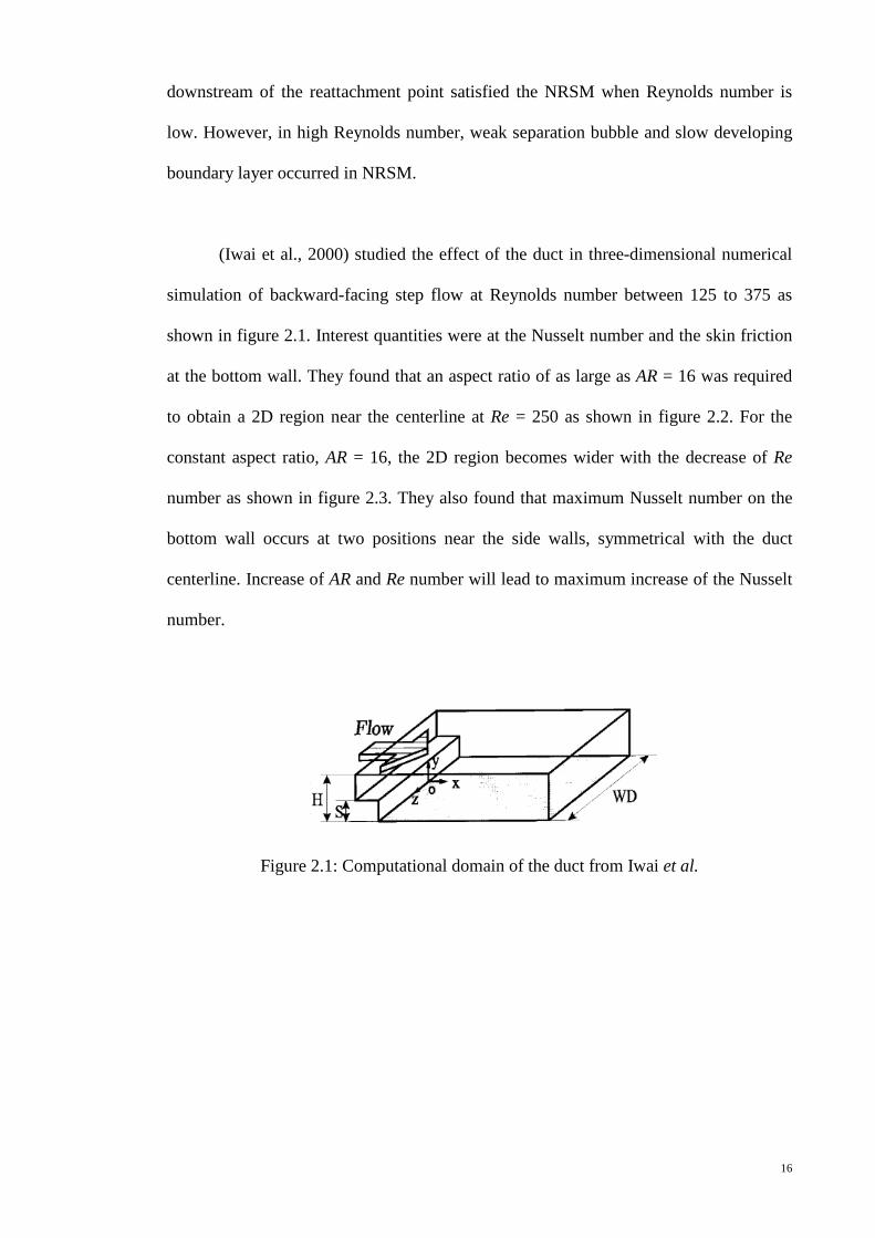
(Iwai et al., 2000) studied the effect of the duct in three-dimensional numerical

simulation of backward-facing step flow at Reynolds number between 125 to 375 as

shown in figure 2.1. Interest quantities were at the Nusselt number and the skin friction

at the bottom wall. They found that an aspect ratio of as large as AR = 16 was required

to obtain a 2D region near the centerline at Re = 250 as shown in figure 2.2. For the

constant aspect ratio, AR = 16, the 2D region becomes wider with the decrease of Re

number as shown in figure 2.3. They also found that maximum Nusselt number on the

bottom wall occurs at two positions near the side walls, symmetrical with the duct

centerline. Increase of AR and Re number will lead to maximum increase of the Nusselt

number.

Figure 2.1: Computational domain of the duct from Iwai et al.

17

(Kim and Baik, 2004) developed a three-dimensional computational fluid

dynamics model with renormalization group (RNG) k-ԑ turbulence scheme to study the

effects of ambient wind direction on flow and dispersion around a group of buildings.

Three flow patterns have been studied numerically such as a portal vortex generated

behind the east wall of the upwind building is symmetric about the center of the street

canyon, a portal vortex generated behind the east wall of the upwind building with its

horizontal axis is not perpendicular to the ambient wind direction and the footprints of a

portal vortex are located behind both the east and north walls of the upwind building. In

their investigation, they stated the numerical models that are suitable for simulation of

urban flow; large-eddy simulation (LES) and Reynolds-averaged Navier-Stokes

equation (RANS). LES is less applied as it requires expensive computing times and

RANS is considered as it widely applied in urban flow and diffusion search. The three-

dimensional CFD model with RNG k-ԑ turbulence is compared with standard k-ԑ

turbulent. They found that the changes in ambient wind direction can highly affect mean

flow circulation and spatial distribution of passive pollutants.

Figure 2.3: Cf contours on the bottom wall (AR = 16)

Figure 2.2: Nusselt number contours on the bottom wall (AR = 16)

18

(Barton, 1997) studied different types of laminar flows which consist of particle-

laden flow, particle-laden flow with heat transfer, single-phase flow with heat transfer,

particle-laden flow with heat transfer and related thermal properties for a backward-

facing step geometry. Eulerian-Lagrangian approach is used in the modeling and the

thermal properties measured are buoyancy and the thermophoresis effect. In the

investigation, the flow particle tends to generate stronger upper and lower recirculation

regions as the particles increase the inertia of the free-stream by overshooting the

streamlines at the expansion. Also, as the particles are gaining momentum, the increases

in inertia in free stream causes stronger recirculation. Finally, higher heat capacities of

the particles successfully augmented the heat capacity of the liquid and further reduce

the temperature in the flowing mixture.

(Chen et al., 2006a) investigate numerically 2 dimensional backward facing

steps using low Reynolds number, incompressible and steady flowing fluid. The lattice

Boltzmann method is utilized in this simulation. A square blockage is placed behind the

sudden expansion to enhance the heat transfer and uniformity of the fluid flow. It was

found that the numerical simulation of temperature field and velocity do agree with the

experimental and numerical results. Figure 2.4 shows the velocity field with square

blockage.

Figure 2.4: Velocity field with square blockage (ER = 2, Re = 105).

19

(Koutmos and Mavridis, 1997) reported a computational study on unsteady

separated flow for different geometries. Time dependent Nevier Stroke equation was

used in the study by using 2 dimensional model. The simulation is performed by using

standard K-epsilon model and Large eddy simulation (LES). The numerical

investigation on backward facing step is executed under low and high Reynolds

number. It was found that the time dependent formulation is better than the steady state

standard k-epsilon model.

(Togun et al., 2011) studied experimentally the effect of step height on heat

transfer to outward expanded air flow stream in a concentric annular passage. The

experiment was done with Re number range from 17050 to 44545, heat flux from 719

W/m2 to 2098 W/m2 and step heights, s = 0, 6mm, 14.5mm, and 18.5mm. They found

that the increase of flow and step height reduces the surface temperature until the lowest

temperature is achieved where reattachment point is located then it increases (figure

2.5). The local heat transfer coefficient (hx) increases with Re number for all cases with

or without step height.

Figure 2.5: Variation of the surface temperature with axial

distance for (q = 2098 W/m2, Re = 44545).

20

(Kolaczkowski et al., 2007) in thier study, offers how to select either a two-

dimensional (2–D), or a three-dimensional model (3–D). They found that the model

with symmetry could be assumed in the tangential direction (axisymmetric option in

FLUENT) and the model with parallel plates, where the gap between the plates is very

much smaller than the width of the plates, could use 2–D model. A model of gas flow in

circular tube, and in a square channel require 3–D model. 3–D requires more

computational resource and it is more complex than 2–D.

(Rajesh Kanna and Manab Kumar, 2006) studied the conjugate heat transfer

characteristic in backward-facing step flow. They studied the effect of Reynolds number

Re, Prandtl number Pr, thermal conductivity ratio, k and thickness of the slab b on the

local Nusselt number by using Alternating Direction Implicit (ADI) discretization

method with centered space. High thermal gradients are observed near the reattachment

location in the solid region shown in figure 2.6. The peak Nu occurs at the downstream

to the reattachment location and at the same location considered for the k values.

Figure 2.6: Effect of Re, Pr, k and b on the local Nusselt number.

21

(Wu et al., 2002) experimentally investigated the mixed convection heat transfer

through vertical annular passage by using water instead of air (Kim et al., 2002) as

flowing fluid. Inner surface was heated uniformly to determine the condition of

turbulence, buoyancy-influence and heat transfer to upward and downward flow. They

found that by increasing buoyancy influence, heat transfer and turbulence production

intensity enhances. They also found that the effect of buoyancy in annular tube is

weaker than that in the circular tube. When heating is applied, laminar flow is changed

to turbulent flow due to the presence of strong buoyancy influence which causes

effective heat transfer enhancement.

(Rouizi et al., 2009) studied numerically the effect of reducing size of the model

on 2–D steady incompressible laminar flows. The objective is to build low-order model

that will fit the original ones. Case of backward-facing step is considered as its

geometry could be simply meshed. Identification technique was derived from the Modal

Identification Method. It can be concluded that a reduced order of model can satisfy the

tests based on computation with other Reynolds number.

(Lee et al., 2011) conducted experiment and numerically studied the heat

transfer and fluid flow properties in circular tube at a uniform wall temperature. Areas

of interest are separated, recirculated and reattached regions produced by an

axisymmetric abrupt expansion and contraction. Diameter ratio of d/D = 0.4 and

Reynolds numbers range from 4,300 – 44,500 are applied. In experimental

investigation, balance-type isothermal heat flux gage was used to measure local heat

transfer coefficients. In numerical investigation, a model of two-equation turbulence

was used. The model shown in figure 2.7 is designed by using the Reynolds-averaged

Navier-Stokes equations, and energy equation for steady, incompressible,

22

axissymmetric and turbulent flow. SIMPLE algorithm was used and second-order

upwind technique was applied to the convective fluxes in the momentum. They found

that a minimum Nusselt number occurs at about 1 step height from the abrupt expansion

step shown in figure 2.8, and the value is up to 1.4 times as high as the fully developed

value. They also found that the reattachment point has strong relationship with the

downstream Reynolds number, which later agreed with the location of maximum

Nusselt number.

(Goldstein et al., 1970) studied experimentally the laminar air-flow in a

downstream-facing step. The observer were interested in visual observations of smoke

filaments in the viscous layer qualitative velocity fluctuation measurements and mean

velocity profiles. Step height varies from 0.36 to 1.02 cm, free steam velocity varies as

0.61 – 2.44 m/s and 0.16 – 0.51 cm in boundary layer displacement thickness at the

step. They found that the laminar reattachment length depends on Reynolds number and

Figure 2.8: Distribution of local Nusselt number in the axisymmetric abrupt expansion for d/D = 0.4.

Figure 2.7: Computational domain in the plane with a non-uniform grid distribution.

23

boundary layer. The shape of the velocity profile at reattachment is found to be similar

to the shape of a laminar boundary layer profile at separation and the boundary layer

profiles downstream of reattachment are similar to those in a laminar boundary layer

developing toward separation except that they are traversed in the reverse sense.

(Zhang, 2003) investigated turbulent flows in constricted conduits with low

Reynolds number. A model of three-dimensional complex conduits was designed, with

variation of renormalization (RNG) k-epsilon and k-omega, to allow incompressible

laminar-to-turbulent fluid flow through it and comparison has been made for different

RNG cases. They found that, both k-epsilon and k-omega model increases the flow

instabilities after tubular constrictions, thus fail to the behavior of laminar flow at low

Reynolds numbers. The low-Reynolds-number (LRN) k-epsilon model is unable to

simulate the transition to turbulent flow and it requires high computational resources

due to the slower convergence. LRN k-epsilon model is adopted well in complex 3–D

tubular flows and able to reproduce the laminar, transition and fully turbulent flows and

even could predict the maximum turbulence fluctuations quite well. It can be concluded

that the LRN k-omega model is suitable for simulation of laminar-transitional-turbulent

flows in the constricted tube.

(Furuichi et al., 2004) investigated experimentally in a large-scale structure of

backward-facing step flow by using an advanced multi-point LDV. The advanced multi-

point LDV has a 1–bit FFT where it is specialized in the time resolution and

measurement in the near wall area. LDV system was used to measure the spatio-

temporal velocity fields around the separated shear layer and reattachment region of

two-dimensional backward facing step. The channel of water, 2300mm length and

expansion ratio, ER=1.5 was used, with Reynolds number fixed as 5000 and turbulent

24

intensity of 0.6%. They found that the moving path of the vortex shedding from

separated shear layer to the reattachment region shows two patterns, one is moving to

near the wall region and the other is moving in the middle of the step height at the

reattachment region. They also found that the turbulence due to reattachment

phenomenon moves from reattachment region to separated shear layer by recirculation

flow. They proposed a self-excitation motion to be a model of large-scale fluctuation.

(Uruba et al., 2007) investigated experimentally on a backward facing step in a

flow through a narrow channel by means of suction or blowing. The flow is set to

Reynolds number 50000 and the intensity of the suction/blowing coefficient was

maintained at -0.035 to 0.035. Preliminary results show that both suction and blowing

can cut down the length of the separation zone to around one third of its result. The 3D

vortex structures close to the step are easily affected by suction compared to blowing.

(Chun and Sung, 1996) studied experimentally the effect of local forcing on flow

structures over a backward-facing step, with a sinusoidal velocity fluctuation which was

applied through a thin-slit near separation line. The experiment was carried out with

Reynolds number varied from 13,000 to 33,000, forcing amplitude, Ao from 0 to 0.07

and forcing frequency, StH from 0 to 5.0. They found that the forcing frequency was

higher than the critical value and the reattachment length was larger than that of the

unforced flow. They also found that the most effective forcing frequency to minimize

the reduction of the reattachment length is close to the vortex shedding frequency of the

unforced flow.

(Armaly et al., 1983b) investigate the backward facing step experimentally and

numerically in a 2 dimensional channel. The range of Reynold number used in the

25

investigation starting from 70 to 8000. The aspect ratio (1:36) was selected to ensure the

fully developed flow. It was shown experimentally that the downstream of the step

remain 2 dimensional for low and high Reynolds numbers only. The performed

investigation also had included numerical prediction for comparisons. It was reported

that as long as the flow maintained its 2 dimensional status in the experiments, both

numerical and experiment results shown good and fair agreement.

(Tota, 2009) studied a turbulent flow over a backward-facing step simulated by

FLOW-3D. A model of Renormalization-group (RNG) k-ε was used with two Reynolds

numbers involved, Reh=5100 and Reh=44000. The numerical results were compared

with the experimental results and showed good agreement. The study observed the

dependency of the turbulent mixing length parameter, tlen in the RNG model. The

model was designed in two dimensional as shown in figure 2.9 where the third-order

upstream advection scheme and GMRES iterative solver were used to solve momentum

and Poisson’s equation for pressure respectively. They found that with the increase of

the value of tlen the velocity profiles move close to the experimental results as shown in

figure 2.10. They also found the reattachment length for tlen=7% is the nearest to the

experimental result whereas tlen=3.5% indicates incorrect result. The streamwise

velocity profiles showed better result after grid refinement applied as shown in figure 2.

11. It can be said that with increase of the value of tlen the turbulent dissipation

decreases. In brief, it was found that there is a value of tlen beyond which mean flow

parameters are not affected.

Figure 2.9: 2–D Computational domain for Re=44000.

26

(Yamamoto et al., 1979) studied the heat transfer characteristics in external

flows over rectangular cavities where the bottom walls were heated at a uniform heat

flux while the other two cavity walls were insulated. They observed that the effects of

the reattachment of separated flow and vortex flow in the cavity on heat transfer were

unexpectedly large. It also found that heat transfer did no always decrease

monotonically with an increase of aspect (depth-width) ratio, in the flow range of

laminar or turbulent.

Figure 2.10: Streamwise velocity Re=5100, x/h=4.

Figure 2.11: Grip refinement: Streamwise velocity profiles for tlen=7% (a) x/h=1.33 (b) 2.66.

27

(Hsu and Chou, 1997) studied numerically hydrodynamic properties of

viscoelastic fluid on a backward-facing step. The study was performed with two-

dimensional, incompressible laminar flow of a second-grade viscoelastic fluid. They

also studied the “overshoot” phenomena, where the development of the main

recirculation zone experiences enlargement first and later shrinkage. The combination

of the line-Gauss-Seidel (LGS) method and alternating direction implicit (ADI) was

applied. They found that, smaller elastic number causing larger main recirculation zone

and longer reattachment length under same Reynolds number. They revealed that the

“overshoot” phenomena is absence in the flow for Newtonian fluids. The secondary

recirculation zone appears at a steady state at Re=75 and elastic number, E=0.001, and

disappears before reaching a steady state for smaller Reynolds and elastic number flow

as shown in figure 2.12.

(Nait Bouda et al., 2008) studied numerically and experimentally a turbulent

wall jet flow over a backward-facing step. Laser Doppler anemometry was applied to

provide better understanding of turbulent flow. As for numerical investigation, two-

Figure 2.12: The effect of the Reynolds number on the reattachment length for E=0.001.

28

dimensional Reynolds Averaged Navier-Stokes (RANS) equation was implemented.

They found that the comparison between experiment and numerical results showed a

good agreement for the mean and turbulent flow fields. However, in the external region

where the turbulent intensity is highly counted, there appears some disagreement due to

the effect of large eddies and slow external motion. The numerical results revealed two

bubbles existence in the recirculation zone. The flow relaxation is found to form more

quickly in the external region rather than internal region.

(Abbassi and Ben Nassrallah, 2007) studied numerically the laminar flow of

magnethydrodynamic (MHD) in backward-facing step. The simulations are performed

for Reynolds number less than Re=380, Stuart number, N, the ratio of electromagnetic

force to inertia force, from 0 to 0.2 and Prandtl number, Pr from 0.02 to 7. They found

that Nusselt number, increases with the increase of Stuart number, N as shown in

figure 2.13. For low Prandtl numbers, heat transfer is not practically dependant by

magnetic field, but depends essentially by diffusion mode. In downstream region, out of

the recirculation zone, the basic flow is damped by magnetic effects, while acceleration

of the flow occurs in near walls.

Figure 2.13: Variation of total averaged Nusselt number as function of Stuart numbers Re=380.

29

(Mohammed et al., 2011) studied the microchannel heat sink (MCHS) made out

of different geometries; one of them is with step. 3 dimensional numerical simulation is

used to solve the conjugate heat transfer governing equations by utilizing Finite Volume

Method. Finite-volume method (FVM) was used to convert the governing equations to

algebraic equations accomplished by using hybrid differencing scheme. The SIMPLE

algorithm was used to enforce mass conservation and to obtain pressure field. Water is

used as working fluid in the simulation and the performance is evaluated based on

pressure drop, wall shear stress, friction factor, heat transfer coefficient and temperature

profile. The step MCHS is the best channel for the hydraulic performance with

moderate degradation of heat transfer compared to conventional straight MCHS.

(Yang et al., 2005) has investigated numerically the homogenous shear flow and

backward-facing step flow with a few linear and non-linear turbulence models. Two

linear models were used in the investigation, such as the standard k–ε model and non-

equilibrium model whereas the non-linear models involves are three quadratic models

from Speziale, Shih, Zhu and Lumley and Huang and also the cubic model of Craft,

Launder and Suga. They found that, under fully developed turbulent flow over

backward-facing step, the non-linear models offers better agreement than linear models.

This is mainly due to the contributions of those non-linear terms representing the

anisotropy of the normal Reynolds stresses.

(Kumar and Dhiman, 2012) numerically studied backward-facing step of

laminar forced convection flow on a circular cylinder for the Reynolds number range 1-

200 and Prandtl number of 0.71. The simulation is conducted using FLUENT and

investigation on the flow and thermal fields are being focused on no temperature

30

dependency. The geometry has been done by GAMBIT consisting of both uniform and

non-uniform grid distribution. The QUICK scheme has been used for momentum and

thermal energy equations and SIMPLE scheme is used for pressure and velocity

equations. It can be found that the insertion of a circular cylinder at a correct position is

really helpful in controlling the velocity field of the backward-facing flow.

(Bsebsu and Bede, 2002) studied theoretically the heat transfer characteristics

of down flow in the single-phase forced-convection with narrow vertical annuli sub-

channels (WWR-M2 channel) using THMOD2 code. The main objective of this

study is to investigate in the turbulent flow region, the applicability of existing

heat transfer equations in the narrow vertical annuli channel, which is modeling

and simulating sub-channel of 3 mm spacing (gap) and 600 mm in active length in

the fuel elements for thermal hydraulic analysis tasks of the WWR-M2 research

reactor or any other type. As a result, it was revealed that by use of equivalent

hydraulic diameter, existing correlations are applicable to a WWR-M2 channel as

narrow as 3 mm in gap for turbulent flow though the precision and Reynolds

number are different among the heat transfer correlations. A new heat transfer

equation for sub-channels of WWR-M2 channel heated at one side or both sides

has been proposed.

(Ota and Kon, 1979) studied the heat transfer measurements in the separated,

reattached and redeveloped regions of the two dimensional airflow on a flat plate with

blunt leading edge. The test plate (20 mm thick, 100 mm wide and 400 mm long) was

made from a stainless steel sheet (0.05 mm thick and 100 mm wide), Bakelite and

plywood. Heating of the plate was done by mean of electric current to both sides of the

plate causing an axisymmetric of flow and temperature fields involved. Heat flux was

31

controlled with sliders and the temperatures on the heating surface were measured

with 0.07 mm copper – constant thermocouple soldered on the back of the stainless

steel sheet. The experiments were carried out under the condition of constant heat flux.

The flow reattachment occurs at about four plate thickness downstream from the leading

edge and the heat transfer coefficient becomes maximum at that point. This behavior is

dependent on the Reynolds number which ranged from 2720 to 17900 in this

investigation. It was found that the heat transfer coefficient increases sharply near the

leading edge.

(Aung et al., 1985) presented theoretical results concerning hydrodynamics and

heat transfer to laminar flow passed through a backward step. Computations were

carried out using the stream function vortices forms of the elliptic partial differential

equations to calculate temperature profiles and local Stanton numbers .The available

results indicate that the shear layer and reattachment length, when normalized by the

step height increases with Reynolds number in the range of 25 <Re < 850.

(Q.Li, 2002) investigated experimentally the convective heat transfer and flow

characteristics in a tube with a constant heat flux at the wall. From data collected on

nanofluids composed of water and Cu, TiO2 and Al2O3 particles, they proposed

empirical correlations for the Nusselt number in both laminar and turbulent flows.

(D.Wen, 2004) investigated the heat transfer performance of water - Al2O3

mixture under laminar flow regime in a copper tube with 4.5 mm inner diameter. They

found that the convective heat transfer coefficient increases with increasing Reynolds

number and particles concentration. Furthermore, the improvement of the heat transfer

coefficient was large in the entrance region of the horizontal heated tube.

32

(Y.Yang, 2005) measured the convective heat transfer coefficient of nanofluids

composed of transmission flu ids and graphitic-based nanoparticles. Results from the

above experimental works have shown that the presence of nanoparticles produces a

clear increase of heat transfer. The nanofluids give a higher heat transfer coefficient than

the base fluid irrespective of Reynolds number, and such enhancement becomes more

significant with an increase of particle concentration.

(R.BenMansour, 2009) studied numerically the conjugate heat transfer to

laminar mixed convection flow of Al 2O3-water nanofluid in a uniformly heated inclined

tube. They found that the presence of nanoparticles intensifies the buoyancy -induced

secondary flow, especially in the developing region. Their results also show an

augmentation of the heat transfer coefficient and a decrease of the wall friction when

using nanofluids.

(S.Z.Heris, 2006) investigated experimentally the convective heat transfer

coefficient of Al2O3-water and CuO-water nanofluids for laminar flow in an annular

tube under a constant wall temperature boundary condition. Their results have shown

that the heat transfer coefficient increases with an increasing Peclet number and

increasing particle volume concentrations while Al2O3-water nanofl uid have shown

larger heat transfer enhancement than CuO-water nanofluid.

(Bianco et al., 2009) investigated numerically the heat transfer of nanofluids in

circular tubes. Forced convection flow of water and aluminium oxide nano particle

mixture is subjected to uniform surface temperature and constant heat flux at surface of

the tube. It was found that the convective heat transfer coefficients to nanofluids are

higher than that of the base fluid. The result also shows the heat transfer enhancement

with higher particle concentration of nanofluids but wall shear stress increases as well.

It was reported in this case that increment in Reynolds number enhances the heat

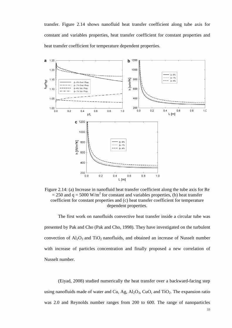
33

transfer. Figure 2.14 shows nanofluid heat transfer coefficient along tube axis for

constant and variables properties, heat transfer coefficient for constant properties and

heat transfer coefficient for temperature dependent properties.

Figure 2.14: (a) Increase in nanofluid heat transfer coefficient along the tube axis for Re

= 250 and q = 5000 W/m2 for constant and variables properties, (b) heat transfer coefficient for constant properties and (c) heat transfer coefficient for temperature

dependent properties.

The first work on nanofluids convective heat transfer inside a circular tube was

presented by Pak and Cho (Pak and Cho, 1998). They have investigated on the turbulent

convection of Al2O3 and TiO2 nanofluids, and obtained an increase of Nusselt number

with increase of particles concentration and finally proposed a new correlation of

Nusselt number.

(Eiyad, 2008) studied numerically the heat transfer over a backward-facing step

using nanofluids made of water and Cu, Ag, Al2O3, CuO, and TiO2. The expansion ratio

was 2.0 and Reynolds number ranges from 200 to 600. The range of nanoparticles

34

volume fraction was 0 ≤ volume fraction ≤ 0.2 and the Prandtl number of the base fluid

(water) was kept constant at 6.2. The flow was assumed Newtonian, two-dimensional,

steady, incompressible, and the base fluid and the nanoparticles were assumed in

thermal equilibrium and no slip occurred. The SIMPLE algorithm was used and second-

order central difference is applied in the diffusion of momentum and energy equations.

A second-order upwind differencing scheme is also applied in terms of convective flow.

They found that Nusselt number inside the recirculation zone is highly dependent on the

thermophysical properties of the nanoparticles, and independent of Reynolds number.

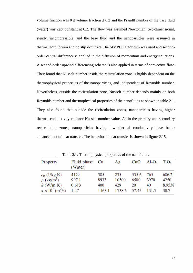
Nevertheless, outside the recirculation zone, Nusselt number depends mainly on both

Reynolds number and thermophysical properties of the nanofluids as shown in table 2.1.

They also found that outside the recirculation zones, nanoparticles having higher

thermal conductivity enhance Nusselt number value. As in the primary and secondary

recirculation zones, nanoparticles having low thermal conductivity have better

enhancement of heat transfer. The behavior of heat transfer is shown in figure 2.15.

Table 2.1: Thermophysical properties of the nanofluids.

35

Nowadays there is a marked increase in research activities in this heat transfer

area, as reviewed in (Murshed et al., 2008), (Kakaç and Pramuanjaroenkij,

2009) and (Das et al., 2006a). A good amount of nanofluids researches is dedicated to

the investigation of thermophysical properties, while a relatively smaller amount of

them is focused on nanofluids convection heat transfer (Murshed et al., 2008), (Das et

al., 2006b) and (Pak and Cho, 1998).

To use nanofluids in heat transfer devices, their higher thermal conductivity is an

encouraging feature, though not a definitive evidence of their applicability. To have a

conclusive picture about the utilization of nanofluids in heat transfer applications, it is

necessary to show their superior performances under convective conditions. In the last

years, different researcher (Pak and Cho, 1998), (Xuan and Li, 2003), (Wen and Ding,

2004), (Zeinali Heris et al., 2007), (Zeinali Heris et al., 2006), (Williams et al.,

2008), (Rea et al., 2009), (Hwang et al., 2009) and (Duangthongsuk and Wongwises,

2009) have focused on the experimental investigation, in both laminar (Wen and Ding,

2004), (Zeinali Heris et al., 2007), (Zeinali Heris et al., 2006), (Rea et al., 2009)

and (Hwang et al., 2009) and turbulent regimes (Pak and Cho, 1998), (Xuan and Li,

Figure 2.15: Nusselt number distribution using different types of nanoparticles, Re = 400, u = 0.1. (a) Top wall and (b) Bottom wall.

36

2003), (Williams et al., 2008) and (Duangthongsuk and Wongwises, 2009), of

nanofluids convection.

37

CHAPTER 3: Methodology

Present research work is complied into two parts. The first section is planned to

gather results of investigation on various numerical model parameters and compare with

the experimental results obtained previously. The results were then being verified by

using different techniques like mesh independent study, surface roughness study and the

effect of various viscous models. The second part of the research was focused on the

numerical simulation of preliminary experimental setup by using the acquired

knowledge. The numerical simulations were conducted by using computational fluid

dynamic package (Fluent). The numerical simulation on heat transfer characteristics

over a considerable number of parameters were carried out; including wall heat flux,

fluid flow velocity, separation step height and various working fluids.

3.1 Numerical simulation of air flow in an annular passage

An experiment was conducted before the numerical simulations to verify the

accuracy and reliability of numerical simulation results. Figure 3.1 shows the

experimental setup conducted by (Togun et al., 2011). The experimental investigation

was focused on the effect of separation flow on the local and average convection heat

transfer. The experimental set-up consists of concentric tubes to form annular passage

with a sudden reduction in passage cross-section created by the variations of outer tube

diameter at the annular entrance section. The outer tube of test section was made of

aluminium having 83 mm inside diameter and 600 mm heated length, which was

subjected to a constant wall heat flux boundary condition. The investigation was

performed in a Re range of 17050–44545 which fall in turbulence flow region and

many industrial applications adopted turbulent flow in cooling and heating processes.

38

The heat flux is varied from 719 W/m2 to 2098 W/m2 and the enhancement of step

heights were, s = 0 (without step), 6 mm, 14.5 mm and 18.5 mm, which refer to d/D = 1,

1.16, 1.53 and 1.80, respectively. The schematic drawing of the annular sudden

expansion pipe flow is presented graphically in Figure 3.2 and the dimensions of

experimental setup are summarized in table 3.1.

Figure 3.1: Experiment setup conducted by Togun et al.

Figure 3.2: Schematic diagram of flow in the annular sudden expansion passage (Togun et al., 2011).

39

Table 3.1: Dimensions of experimental setup. Inner tube Diameter of entrance section Diameter at test section

Di=22 mm D=(83, 71, 54, 46) mm d=83 mm

L=1500 mm L=500 mm L=600 mm

The inner or outer surface temperatures of the annular pipes with sudden

expansion can be influenced by many parameters, such as flow velocity, surface heat

flux, and the step heights. The fluid utilized to conduct heat transfer in these

experiments is air. The inlet and outlet diameter of the pipe are 46 and 83 mm

respectively, the inner tube diameter of the annular pipe is 22 mm. In the simulations, 4

different cases were considered in an annular passage. The surface heat flux of the

annular pipe is selected as 2098 W/m2 with variable Reynolds numbers between 17,050

to 44,545 and D/d = 1.8 which is corresponding to 18.5 mm of step height. The

numerical simulation parameters are summarized in table 3.2. Only Reynolds number of

17,050 and heat flux equal to 2098W/m2 are considered experimentally to verify the

numerical results.

Table 3.2: Experimental parameters.

Variable Parameter Value

Inlet dimension 0.012 m

Outlet dimension 0.0305 m

Reynolds number 1, Re1 17,050

Reynolds number 2, Re2 30,720

Reynolds number 3, Re3 39,993

Reynolds number 4, Re4 45,545

40

The geometry invention of the tube has been designed by using GAMBIT

2.2.30. The geometry of the tube was designed based on the exact experimental tube

dimensions (Togun et al., 2011) (figure 3.3 and figure 3.4). As the geometry of the tube

is symmetrical the geometry was designed by half (axissymetric), using 2–D model, as

suggested in (Kolaczkowski et al., 2007). Table 3.2 and table 3.3 show the dimensions

of the model drawn in GAMBIT. Models are designed with four different step heights,

s=0, 6mm, 14.5mm and18.5mm.

Figure 3.3: Geometry and dimensions of the model.

Figure 3.4: Geometry and boundary conditions are drawn by using GAMBIT.

Table 3.3: Dimensions of the entrance section and test section.

Step height, s (mm) Diameter at entrance section, D (mm)

Diameter at test section, d (mm)

0 30.5 30.5

6.0 24.5 30.5

14.5 16.0 30.5

18.5 12.0 30.5

Outer tube = 500mm Inner tube = 600mm

D= varies (mm) d= constant (mm)

s (mm)

q= constant (mm)

41

Flow Chart of Methodology

Compare the experimental and numerical simulation result (analysis

both result for verification)

Complete numerical simulation for parameters that have been identified over

the proposed geometry

Determine the geometry (step), type of fluid and range of flow velocity (Reynolds number).

Preliminary design – CFD simulation of different geometrical configurations

Feasibility study and conceptual design of different geometrical configurations of annular passage

Interpretations, implications and conclusions of obtained experimental &

CFD simulation results

42

3.1.1 Computational Fluid Dynamic (CFD)

Fluid flow in a physical domain is governed by the laws of conservation of mass

and momentum. These conservation laws, for steady flows in a closed conduit two-

dimensional domain can be stated as follows.

Continuity equation:

( ) ( ) 0=∂∂

+∂∂ v

yu

xρρ

(1)

Momentum conservation equations:

( ) ( )

∂∂

+∂∂

+∂∂

−=∂∂

+∂∂

2

2

2

2

yu

xu

xpuv

yuu

xµρρ

(2)

( ) ( )

∂∂

+∂∂

+∂∂

−=∂∂

+∂∂

2

2

2

2

yv

xv

ypvv

yvu

xµρρ

(3)

where u and v are the velocity components in the x and y directions. These

equations are discretised by using the finite volume scheme.

Flow-solver formulates the principle of mass, momentum and energy

conservation in partial differential equation forms on the basis of two dimensional

Navier-Stokes equations. Navier-Stokes equations are discretized along with cells in the

computational domain by finite volume method.

In all of the above references, the step in backward facing cases is vertical to the

stepped wall. In these geometries, there is a sudden expansion or contraction in the

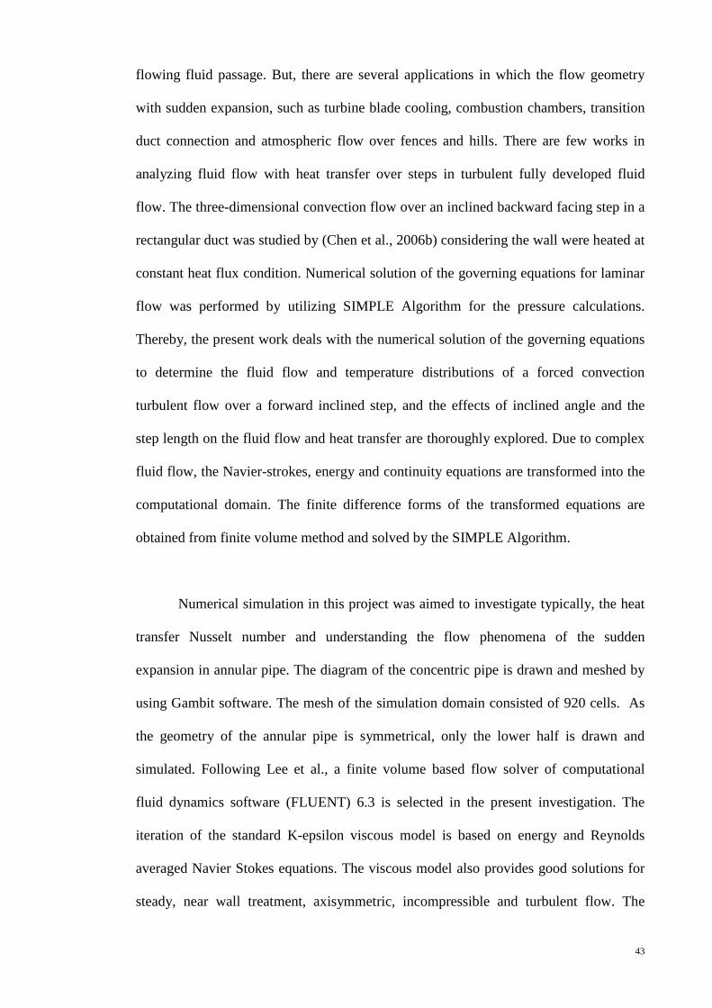
43

flowing fluid passage. But, there are several applications in which the flow geometry

with sudden expansion, such as turbine blade cooling, combustion chambers, transition

duct connection and atmospheric flow over fences and hills. There are few works in

analyzing fluid flow with heat transfer over steps in turbulent fully developed fluid

flow. The three-dimensional convection flow over an inclined backward facing step in a

rectangular duct was studied by (Chen et al., 2006b) considering the wall were heated at

constant heat flux condition. Numerical solution of the governing equations for laminar

flow was performed by utilizing SIMPLE Algorithm for the pressure calculations.

Thereby, the present work deals with the numerical solution of the governing equations

to determine the fluid flow and temperature distributions of a forced convection

turbulent flow over a forward inclined step, and the effects of inclined angle and the

step length on the fluid flow and heat transfer are thoroughly explored. Due to complex

fluid flow, the Navier-strokes, energy and continuity equations are transformed into the

computational domain. The finite difference forms of the transformed equations are

obtained from finite volume method and solved by the SIMPLE Algorithm.

Numerical simulation in this project was aimed to investigate typically, the heat

transfer Nusselt number and understanding the flow phenomena of the sudden

expansion in annular pipe. The diagram of the concentric pipe is drawn and meshed by

using Gambit software. The mesh of the simulation domain consisted of 920 cells. As

the geometry of the annular pipe is symmetrical, only the lower half is drawn and

simulated. Following Lee et al., a finite volume based flow solver of computational

fluid dynamics software (FLUENT) 6.3 is selected in the present investigation. The

iteration of the standard K-epsilon viscous model is based on energy and Reynolds

averaged Navier Stokes equations. The viscous model also provides good solutions for

steady, near wall treatment, axisymmetric, incompressible and turbulent flow. The

44

second order upwind is used to solve the field variables at the finite volume cell faces

for computing the solution. A SIMPLE algorithm is used to establish coupling between

velocity and pressure. According to (Rahgoshay et al., 2012), the SIMPLE algorithm

links the mass conservation and momentum equations through pressure corrections. Due

to the computational robustness and efficiency in iterating the coupled parameters and

higher order differencing schemes, this algorithm was selected over others. A balance

between computing cost as well as accuracy is achieved by this method in numerical

differentiation of the convective terms, with the linear upwind differencing scheme.

table 3.4 shows the computational conditions of the numerical simulation.

Table 3.4: Computaional conditions.

Computational conditions

Density 1.23 kg/m3 Interpolating scheme (turbulence)

2nd Order Upwind

Viscosity 1.7894 x 10-5 kg/m.s Residual error 1 x 10-4 Pressure 101,325 Pa Inlet Boundary Type Velocity Inlet

Space /Time 2D /Unsteady, 2nd-Order Implicit Reference Frame Absolute

Viscous Model k and ε Reynolds number See Table I

CFD algorithm SIMPLE Outlet Boundary Type Pressure outlet Interpolating

scheme (momentum)

2nd Order Upwind

The properties of air were set to the standard atmosphere values at sea level,

pressure 101, 325 Pa, temperature of 300 K, thermal conductivity 0.03 W/m.K and

specific heat, Cp 1.005 kJ/kg.K. The flow solver used was steady state and pressure

based which associates both the momentum and mass conservation equation. Unsteady

assumption is selected for most cases where convergence can be obtained. Simulations

were performed until the residual values were less than 1 x 10-4.

45

The analysis of the backward-facing step flow was performed by using

FLUENT 6.3.26. Four different Reynolds numbers are tested in the simulation,

Re=17050, 30720, 39992 and 44545, producing fully developed turbulent unsteady flow

and heat flux applied to the inner tube varies from q=719 W/m2, 968 W/m2, 1458 W/m2

and 2098 W/m2. Pressure based solver with 2nd –order implicit unsteady formulation,

with standard k-epsilon (Yakhot and C.G., 1992) equation were applied in defining the

model.

Second order upwind is applied in solving the momentum, turbulent kinetic

energy, turbulent dissipation rate and energy discretizations (Lee et al., 2011). A

coupling between pressure and velocity is established through the SIMPLE algorithm.

The boundary condition of the inlet is defined as velocity inlet, whereas for outlet it is

pressure outlet with turbulent intensity of 7% and turbulent length scale 0.06 m. Fluid

material is air having density of 1.225 kg/m3, Cp=1006.43 J/kg-K, thermal conductivity

0.0242 (W/m-K) and viscosity 1.7894x10-5(kg/m-s). Gravity influence is neglected.

The Reynolds number (Red) can be obtained by the following Eq. (4):

where ρf is the density of the fluid, U is the velocity of the fluid, is the hydraulic

diameter of the annular pipe and μf is the dynamic viscosity of the fluid at film

temperature.

46

The local heat transfer coefficients are calculated using convection heat flux as shown

by Eq. (5):

where qc is the convection heat flux, Tsx is the local surface temperature and Tbx is the

local bulk air temperature.

The local Nusselt number (Nu) can be evaluated by Eq. (6):

where d is the diameter of the pipe and Kf is the thermal conductivity.

Using the equations 4-6, the experimental data for expansion ratio D/d=1.8, Heat

flux q=2098 and reynold number Re=17050 to 44545 were reduced. By using equation

5, the local heat transfer coefficient was calculated and subsequently local nusselt

number was evaluated from equation 6. Nusselt number for turbulent fully develop flow

was then calculated from Dittus-Boelter’s correlation (7). The previously calculated

local Nusselt numbers were divided by nusselt numbers evaluated from Dittus Boelter

correlation to obtain the ratio Nu/Nud (Kreith and Bohn, 2001).

Nud = 0.023 Re 0.8 Pr 0.4 (7)

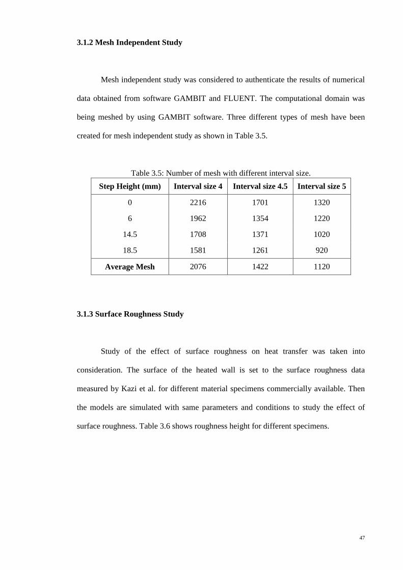
47

3.1.2 Mesh Independent Study

Mesh independent study was considered to authenticate the results of numerical

data obtained from software GAMBIT and FLUENT. The computational domain was

being meshed by using GAMBIT software. Three different types of mesh have been

created for mesh independent study as shown in Table 3.5.

Table 3.5: Number of mesh with different interval size. Step Height (mm) Interval size 4 Interval size 4.5 Interval size 5

0 2216 1701 1320

6 1962 1354 1220

14.5 1708 1371 1020

18.5 1581 1261 920

Average Mesh 2076 1422 1120

3.1.3 Surface Roughness Study

Study of the effect of surface roughness on heat transfer was taken into

consideration. The surface of the heated wall is set to the surface roughness data

measured by Kazi et al. for different material specimens commercially available. Then

the models are simulated with same parameters and conditions to study the effect of

surface roughness. Table 3.6 shows roughness height for different specimens.

48

Table 3.6: Roughness height of the commercially available test specimens (Kazi et al., 2010).

Specimen Roughness Height, µm

Polycarbonate 0.25

SS 316 0.88

Brass 2.3

Aluminium 2.9 3.2 Basefluid and Nanofluid Methodology

A preliminary study on backward facing step of basefluid (water), different

nanofluids and different concentration of nanofluid were conducted using CFD. The

schematic drawing of the annular sudden expansion pipe flow is presented graphically

in Figure 3.5. Figure 3.6 shows the geometry of asymmetry annular test section drawn

in GAMBIT. The inner or outer surface temperature of the annular pipe with sudden

expansion can be influenced by many parameters, such as flow velocity, surface heat

flux, and the step heights. The inlet 33 mm, 39 mm, 52 mm and 60mm, then the outlet

of the tube is 60 mm. The diameter of the inner tube is 20 mm. Table 3.7 and table 3.8

show the dimension of the annular test section with different step heights.

Figure 3.5: Schematic diagram of the annular sudden expansion in annular pipe flow for basefluid and nanofluid.

Di

d D

S

q

0.3 m 1 m

49

Table 3.7: Dimensions of the model. Inner tube Outer tube at entrance section Outer tube at test section

Di=20 mm D=(60, 52, 39, 33) mm d=60 mm

L=1300 mm L=300 mm L=1000 mm

Figure 3.6: Geometry of asymmetry annular test section are drawn by using GAMBIT.

Table 3.8: Dimensions of the entrance section and test section

3.2.1 Thermophysical properties of nanofluids

The numerical data for nanofluid densities were studied by (Brinkman, 1952),

the temperature independent values based on nanoparticle volume fraction were

calculated using equation (8):

Similarly, it has been suggested that the effective specific heat can be calculated

by using equation (9).

Step height, s (mm) Entrance of the tube before expansion, d (mm)

Outlet of the tube after expansion, D (mm)

0 20 20

4 16 20 10.5 9.5 20 13.5 6.5 20

(8)

(9)

50

In this study, dynamic viscosity, µ was considered dependent only on

concentration of nano particles in the basefluid, and the temperature dependency was

neglected.

For the nanaofluids thermal conductivity determination, the same criteria used

by (Khanafer et al., 2003) was introduced. This equation is applicable for the two-phase

mixture containing micro-sized particles. In the absence of any convenient formula for

the calculations of the stagnant thermal conductivity of nanofluids, equation (11) may

approximately apply to obtain a reasonable estimation (Wasp et al., 1977):

where ρ is density, Cp is specific heat, k is thermal conductivity and µ is

dynamic viscosity. Table 3.9 shows the thermophysical properties of nano particles that

were used to calculate the thermophysical properties of different nanofluids.

Table 3.9: Thermophysical properties of nano particles.

Property

Fluid phase

(water)

Nanoparticles

Cu

Ag

CuO

Al2O3

TiO2 Cp (J/kg-K) 4182 385 235 535.6 765 686.2

ρ (kg/m3) 998.2 8933 10500 6500 3970 4250

k (W/m-K) 0.597 400 429 20 40 8.9538

(10)

(11)

51

Table 3.10 shows the thermophysical properties of water-Al2O3 nanofluids at

different concentration. Using the present formulation, several assumptions were made,

such as the flow is consider as single phase model, the concentration of nanofluid is

assume to be constant during the testing and the effect of temperature to the

thermophysical properties is negligible. The thermophysical properties were calculated

using equations 8, 9, 10 and 11. The data were used to run the simulation in order to

investigate the effect of concentration on the behavior and characteristics of water-

Al2O3 nanofluid flowing through various steps height and Reynolds numbers.

Table 3.10: Thermophysical properties of water-Al2O3 nanofluids at different concentration.

Fluid

Volume

concentration (%)

Viscosity, kg/m-s (µ)

Density, kg/m3 (ρ)

Specific

heat, J/kg-K (Cp)

Thermal

conductivity W/m-K (K)

H2O (water) 0% 1.003×10-3 998.2 4182 0.6

Al2O3 - water 1% 1.0886×10-3 1027.9 4147.8 0.6143

Al2O3 - water 2% 1.1988×10-3 1057.6 4113.7 0.6319

Al2O3 - water 3% 1.3337×10-3 1087.4 4079.5 0.6499

Al2O3 - water 4% 1.4933×10-3 1117.1 4045.3 0.6682

The analysis was also conducted by using different types of nanofluids eg: water

based Cu, CuO, Ag, TiO2 and Al2O3. The comparison was done in 1% volumetric

concentration of different nanofluids. The value of the thermophysical properties of the

fluids were calculated by using equations 8, 9, 10 and 11 and presented in table 3.11.

52

Table 3.11: Thermophysical properties of nanofluids with 1% volumetric concentration.

Type of fluid

Density,

kg/m3 (ρ)

Viscosity, kg/m-s (µ)

Thermal conductivity W/m-K (K)

Specific heat J/kg-K (Cp)

Cu - water 1077.5 1.0886×10-3 0.6150 4144

CuO - water 1053.2 1.0886×10-3 0.6135 4145.5

Ag- water 1093.2 1.0886×10-3 0.6150 4142.5

TiO2 - water 1030.7 1.0886×10-3 0.6119 4147

Al2O3 - water 1027.9 1.0886×10-3 0.6143 4147.8

The analysis on the backward-facing step flow was employed using FLUENT

6.3.26. Four different Reynolds numbers Re=17050, 30720, 39992 and 44545 were

simulated in the investigation. Heat flux applied at the test section were q=49050 W/m2.

The analysis was also conducted for different volume fraction range between 0% ≤ φ ≤

4%. The properties calculated were defined in FLUENT’s materials database. The

boundary conditions of the model were defined according to the setting utilized for the

flow separation using air. The working fluids used in the simulation are base fluid

(water) and different nanofluids (with variable thermophysical properties that have been

defined in FLUENT’ material database). Gravity influence is neglected.

53

CHAPTER 4: Results and Discussions

Generally, the presence of backward facing step in the pipe flow shows

reduction of temperature on the inner surface of the pipe. Due to the turbulent flow, the

heat transfer is augmented in some areas. The lowest temperature is obtained at the end

of flow recirculation zone where the flow reattachment happens after the flow separated

at the beginning of the step. The Vector of fluid flow is shown in figure 4.1. After flow

reattachment the fully developed turbulent flow carries the heat though the rest of the

pipe and exhaust as hot air. Figure 4.2 shows the temperature distribution along the pipe

where the colours ranging from blue to red indicate low temperature to high

temperature.

\

Figure 4.1: Vector of air inside the pipe.

54

Figure 4.2: Temperature distribution along the pipe.

4.1 Numerical simulation of air flow in an annular passage

In the simulation process, 4 different cases were considered for flow through an

annular passage. The surface heat fluxes from the annular pipe is selected at 2098 W/m2

with a variable Reynolds number between 17,050 to 44,545 in a given geometry. The

average temperature at Re=17,505 for both numerical and experimental results are

371.77 K and 372.19 K respectively, where the percentage of deviation error is less than

1 %. The temperature versus x/D graph is shown in figure 4.3.

Figure 4.3: The variation of surface temperature with x/D.

55

The evaluated Nusselt numbers for the specific Reynolds numbers are plotted in

figure 4.4. The noticeable trend of the results is the sudden increase in the local Nusselt

number when the fluid flows to the end of the recirculation zone. In a study conducted

by Charwat et al. [10], the obtained result is identical to the present observation due to

the intervallic vortex shedding followed by the reattachment at the corner area of the

recirculation zone. Also, the process of fresh fluid intervallic “filling” and “emptying”

the recirculation zone may contribute to the dramatic increase in Nusselt number.

Lastly, the numerically simulated Nusselt number varationswith x/D at Reynolds

number 17,505 are in reasonable agreement with experimental results representing

location and magnitude of the highest Nusselt number. Observed difference of both

average Nusselt numbers difference are less than 10 %.

Figure 4.4: The graph of Nusselt number versus x/D.

The variation of local Nusselt number ratio (Nu/Nud) with x/D for heat flux

q=2098 W/m2 and expansion ratio D/d=1.8 are presented in figure 4.5. The local

Nusselt number ratio increases to a maximum magnitude then decrease towards the end

56

of the test pipe. The maximum value of local Nusselt number ratio appears between 1

and 2 of x/D for four Reynolds numbers. The highest peak of local Nusselt number

appears in the range of 34.8 to 36.5. The highest local Nusselt number obtained at

Re=44545 which is 4.9% higher than that obtained at turbulent fully developed flow at

Reynolds number Re=17050. The augmentation of heat transfer observed with increase

of Reynolds number where the value of local Nusselt number enhances due to induced

eddies. The region of heat transfer augmentation is found in the distance of four outer

diameters from the expansion.

Figure 4.5. The graph of local Nusselt number/Nusselt number (Dittus-Boelter) versus

x/D.

Figure 4.6 shows the variation of the surface temperature versus distance for

different Reynolds number at heat flux 790 W/m2 and a step height equal to (18.5), i.e.

(d/D = 1.8). Figure 4.6 shows that the surface temperature variation decreases with the

increase of Reynolds number for the same heat flux and step height. Figure 4.7 and

figure 4.8 shows the effect of variation of heat flux on the simulation surface

57

temperature at Reynolds number 17050 and 44545 respectively with step height equal

to (18.5), i.e. (D/d = 1.8). The general shape shows a reduction of surface temperature at

the test section inlet directly behind the step (x = 0). The minimum magnitude of

temperature is obtained at a specific axial position where the flow reattachment takes

place after the separation region due to turbulence augmented heat transfer. Then the

temperature gradually increases along the pipe with the reduction of heat transfer rate. It

is noted that the distance increases with the surface temperature with distance increases

with the increase of heat flux. Thus an optimization analysis of heat exchanger could be

taken as an extension of present investigation.

Figure 4.6 Variation of surface temperature versus distance (for heat flux=790 W/m2,

D/d=1.8).

58

Figure 4.7: Variation of surface temperature versus distance (for re=17050, D/d=1.8).

Figure 4.8: Variation of surface temperature versus distance (for Re=44545, D/d=1.8).

Figure 4.9 shows the variation of surface temperature as a function of distance

with different step heights for Re=39992 and q=2098 W/m2. The entire graph did not

share a common profile, at s=0 and 6 mm, it appears as linear shapes slightly rise of

with surface temperature until the end of the test pipe. On the other hand, in case of

59

s=14.5 mm and 18.5 mm, the curve shows a minimum surface temperature indicating

the presence of reattachment point. For s=0 and 6 mm, the reattachment point could not

be specified as the surface temperature is not having a sudden drop, whereas for s=14.5

mm and 18.5 mm, the reattachment point appears at 0.542 m, where the minimum

surface temperature is obtained. The error of average surface temperature between

experimental and numerical is 1.26 % referring to good numerical approach for

estimating temperature profile. However, for the step heights of 0 and 6 mm, the results

shows almost no fluctuation due to the step heights is too small to induce backward

facing steps.

Figure 4.9: The graph of surface temperature versus distance with different step height (for Re=39992, q=2098 W/m2).

Figure 4.10 representing the local heat transfer coefficient versus distance with

different step height for the case of Re=39992 and q=2098 W/m2. The entire graph did

not share a common profile, where s=0 and 6 mm are maintained, It appears as profile,

with heat transfer coefficient slightly decreasing until the end of the test pipe. But for

60

the step height of s=14.5 mm and 18.5 mm, the hx increases up to a maximum point

(reattachment point), and then decrease slowly. For s=14.5 mm and 18.5 mm, the hx

appears to be similar and overlapping each other, while at s=0 it illustrates higher hx

than s=6 mm. Thus, it opens an avenue for optimization of heat exchangers.

Figure 4.10: The graph of local heat transfer coefficient versus distance with different step height for (Re=39992, q=2098 W/m2).

Figure 4.11 the graph of Nusselt number versus distance with different step

heights at Re=39992 and q=2098 W/m2. The entire graph did not share a common

profile, for s=0 and 6 mm, it appears as linear curve, and for s=14.5 mm and 18.5 mm,

the Nusselt number increases up to a maximum point (reattachment point), and then

decreases slowly. For s=14.5 mm and 18.5 mm, the Nusselt number appears to be

overlapping each other, while at s=0 it illustrates higher Nusselt number than at s=6

mm. It can be concluded that, the effect on Nusselt number is not significant in all cases

when the step heights are varied with ultimately opens up an avenue of optimization of

heat exchangers.

61

Figure 4.11: The graph of Nusselt number versus distance with different step heights (for Re=39992, q=2098 W/m2).

Figure 4.12 represents the surface temperature distribution for different

Reynolds numbers of Re=17050, 30720, 39992 and 44545 for s=18.5 mm and q=2098

W/m2. The reattachment region shows the lowest surface temperature at 300 K for all

Reynolds numbers. The reattachment length simulated is about 0.042 m from the

expansion for all Reynolds numbers. After the fluid passes reattachment region, the

surface temperature increases gradually and the higher temperature is located near the

heated wall approximately at 350 K. The highest temperature is located at the outlet of

the test pipe which is around 383 K.

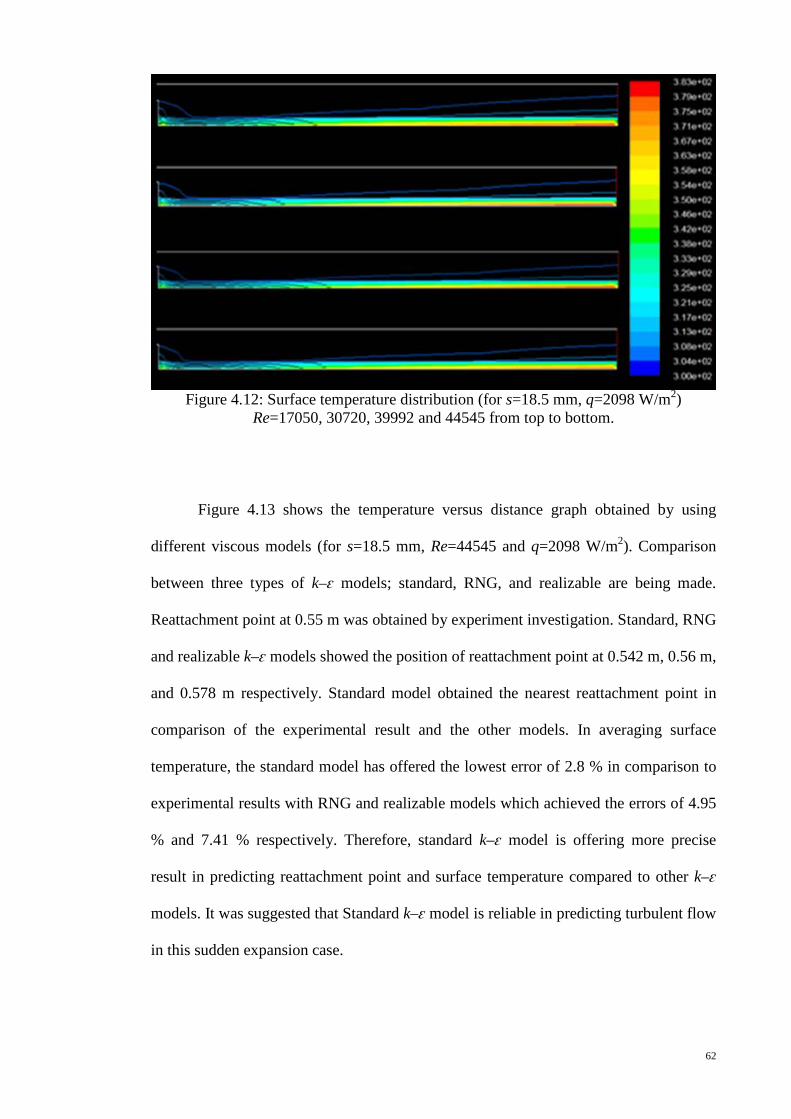
62

Figure 4.12: Surface temperature distribution (for s=18.5 mm, q=2098 W/m2)

Re=17050, 30720, 39992 and 44545 from top to bottom.

Figure 4.13 shows the temperature versus distance graph obtained by using

different viscous models (for s=18.5 mm, Re=44545 and q=2098 W/m2). Comparison

between three types of k–ԑ models; standard, RNG, and realizable are being made.

Reattachment point at 0.55 m was obtained by experiment investigation. Standard, RNG

and realizable k–ԑ models showed the position of reattachment point at 0.542 m, 0.56 m,

and 0.578 m respectively. Standard model obtained the nearest reattachment point in

comparison of the experimental result and the other models. In averaging surface

temperature, the standard model has offered the lowest error of 2.8 % in comparison to

experimental results with RNG and realizable models which achieved the errors of 4.95

% and 7.41 % respectively. Therefore, standard k–ԑ model is offering more precise

result in predicting reattachment point and surface temperature compared to other k–ԑ

models. It was suggested that Standard k–ԑ model is reliable in predicting turbulent flow

in this sudden expansion case.

63

Figure 4.13: The graph of temperature versus distance with different viscous model (for s=18.5 mm, Re=44545 and q=2098 W/m2).

4.1.1 Mesh Independent Study

The mesh independent study shows that with the reduction of meshing interval

sized from 5 to 4.5, the different average temperature is about 10 K at Re=17050. On

the other hand, the reduction of meshing interval size from 4.5 to 4 show only 0.5 K

reduction in average temperature for the same case. It is concluded that the meshing is

good enough for the simulations. Figure 4.14 shows the comparison of average surface

temperature for various interval sizes at s=18.5 mm and q=2098 W/m2. For interval

size=4.5, the data is 2.14 % deviated from the interval size 5 at Reynolds

number=17050, whereas for the interval size of 4.5 and 5, it shows errors of less than

0.1 %. Interval size of 4 offers less deviation compared to other interval sizes, such as

the interval size of 5 which contributes larger error. For the reduction of interval size

64

from 4.5 to 4, the number of meshing element will increase. The result shows the

meshing is good enough to validate the mesh independent study.

Average heat transfer coefficient is being compared for different interval sizes in

figure 4.15. Interval size of 4.5 shows the smallest difference among all the numerical

data. Interval size of 4 and 5 show errors of 2.44 % and 9.76 % respectively compare to

interval size of 4.5 at Reynolds number=39992. Same trend is applied for the Reynolds

number of 30720 and 44545. Finally, the deviation of numerical data for Reynolds

number=17050 is not significant for three interval sizes. It can be conclude that the

interval size of 4 and 4.5 are preferable meshing for heat transfer coefficient

investigation in present case. Figure 4.16 shows the comparison of average Nusselt

number with different interval sizes. Same conclusion can be drawn for the case of

average heat transfer coefficient and average Nusselt number.

Figure 4.14: Comparison of average temperature over various Reynolds numbers at

s=18.5 mm and q=2098 W/m2.

65

Figure 4.15: Comparison of average heat transfer coefficient over various Reynolds

numbers at s=18.5 mm and q=2098 W/m2.

Figure 4.16: Comparison of average Nusselt number over various Reynolds numbers at

s=18.5 mm and q=2098 W/m2.

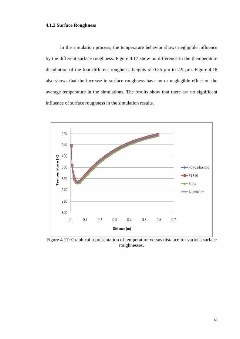
66

4.1.2 Surface Roughness

In the simulation process, the temperature behavior shows negligible influence

by the different surface roughness. Figure 4.17 show no difference in the themperature

distubution of the four different roughness heights of 0.25 µm to 2.9 µm. Figure 4.18

also shows that the increase in surface roughness have no or neglegible effect on the

average temperature in the simulations. The results show that there are no significant

influence of surface roughness in the simulation results.

Figure 4.17: Graphical representation of temperature versus distance for various surface

roughnesses.

67

Figure 4.18: Graph of average temperature versus roughness height for different

materials. 4.2 Numerical simulation of base fluid and nanofluids in an annular passage

Simulation were conducted over a straight annular passage with a different step

height s = 0 and 13.5 mm maintained against expansion ratios of d/D =1 and 1.80

respectively. The test section outer tube for heat flux was constant q=49050 W/m2.

Generally, the surface temperature along the test pipe may be affected by many

variables, such as concentration, heat flux, velocity and the step height of the test pipe.

4.2.1 Numerical simulation of base fluid and nanofluids for 0 step height

The temperature variations at 0 step height simulation are presented graphically

in figure 4.19. There is no separation observed in the present case, after the fully

developed flow reached the heat wall, surface temperature increases along the pipe.

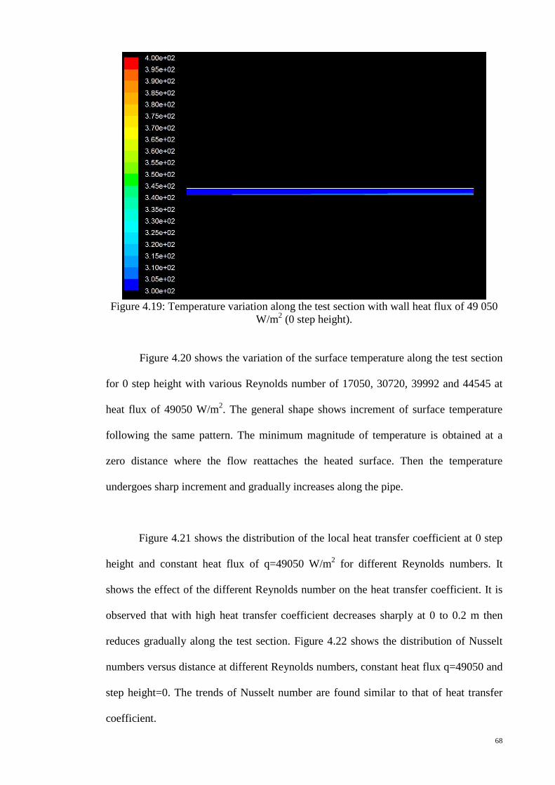
68

Figure 4.19: Temperature variation along the test section with wall heat flux of 49 050

W/m2 (0 step height).

Figure 4.20 shows the variation of the surface temperature along the test section

for 0 step height with various Reynolds number of 17050, 30720, 39992 and 44545 at

heat flux of 49050 W/m2. The general shape shows increment of surface temperature

following the same pattern. The minimum magnitude of temperature is obtained at a

zero distance where the flow reattaches the heated surface. Then the temperature

undergoes sharp increment and gradually increases along the pipe.

Figure 4.21 shows the distribution of the local heat transfer coefficient at 0 step

height and constant heat flux of q=49050 W/m2 for different Reynolds numbers. It

shows the effect of the different Reynolds number on the heat transfer coefficient. It is

observed that with high heat transfer coefficient decreases sharply at 0 to 0.2 m then

reduces gradually along the test section. Figure 4.22 shows the distribution of Nusselt

numbers versus distance at different Reynolds numbers, constant heat flux q=49050 and

step height=0. The trends of Nusselt number are found similar to that of heat transfer

coefficient.

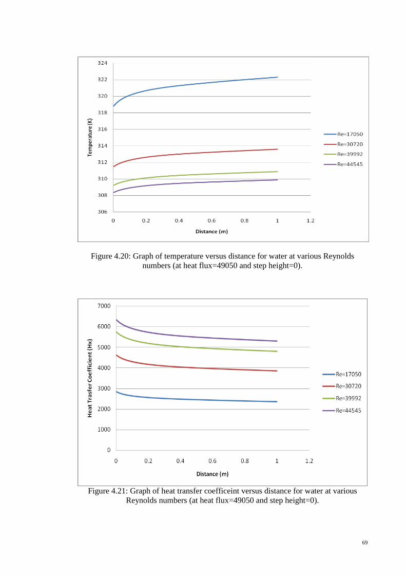
69

Figure 4.20: Graph of temperature versus distance for water at various Reynolds numbers (at heat flux=49050 and step height=0).

Figure 4.21: Graph of heat transfer coefficeint versus distance for water at various

Reynolds numbers (at heat flux=49050 and step height=0).

70

Figure 4.22: Graph of Nusselt number versus distance for water at various Reynolds

numbers (at heat flux=49050 and step height=0).

Further, the simulations were carried out by employing the single phase model

for volume concentrations of φ = 1%, 2%, 3% and 4%, Reynolds number, Re = 17050,

heat flux, q = 49050 W/m2 and at 0 step height. Figure 4.23 presents comparison of

temperature variations at different Al2O3 concentrations of nanofluids. It is observed in

figure 4.23 that the temperature increases with the increase of φ. The curves show

similar pattern for all the concentrations. Figure 4.24 shows the heat transfer coefficient

versus distance for the same concentration parameters. The highest heat transfer

coefficient is obtained at the concentration φ=1% of Al2O3. The heat transfer coefficient

curve decreases when the concentration increases from 1% to 4 %. Figure 4.25 shows

the Nusselt number versus distance for the same oncentration parameters. Again, the 1%

concentration shows the highest Nusselt number. Then, the Nusselt number decreases

when the concentration increases. Both heat transfer coefficient and Nusselt number

shows the similar trend because both temperature different and thermal conductivity

increases with the increase of nano particle concentration in the suspension. Thus

71

overall heat transfer increases with the increase of particle concentration in the

nanofluid.

Figure 4.23: Graph of Temperature versus distance for water Al2O3 nanofluids with

different concentrations (at heat flux of 49050W/m2 and step height=0).

Figure 4.24: Graph of heat transfer coefficient versus distance for water Al2O3

nanofluids with different concentration (heat flux of 49050W/m2, step height=0).

72

Figure 4.25: Graph of nusselt number versus distance for water Al2O3 nanofluids with

different concentrations (at heat flux of 49050W/m2 and step height=0).

4.2.2 Numerical simulation of base fluid and nanofluids at 13.5 mm step height

The temperature variations at 13.5 mm step height simulation are presented

graphically in figure 4.26.

Figure 4.26: Temperature variation along the test section with wall heat flux of 49 050

W/m2 (at 13.5 mm step height).

73

Figure 4.26, shows the variation of the surface temperature along the test section

at 13.5 mm step height with various Reynolds numbers of 17050, 30720, 39992 and

44545 with heat flux of 49050 W/m2. The general shape shows increment of surface

temperature of the same pattern. The minimum magnitude of temperature is obtained at

0.05 m from step where the flow reattachment happens. Then the temperature decreases

to a minimum point then gradually increases along the pipe. Reynolds number of 17050

shows the highest temperature and decreases as the Reynolds number increases due to

augmentation of heat transfer with increase of Reynolds number. The region of heat

transfer augmentations is found to be the distance of ten times diameter of outer

diameter from the expansion.

Figure 4.28 shows the distribution of the local heat transfer coefficient at 13.5

mm step height and constant heat flux of q=49050 W/m2 for different Reynolds

numbers. It shows the effect of the different Reynolds numbers on the heat transfer

coefficient. It started with high heat transfer coefficient and decreases sharply before

0.05 m from the expansion then increases gradually along the test tube. Reynolds

number of 44545 shows the highest heat transfer coefficient which decreases with the

increase of Reynolds number. The heat transfer coefficient increase at 0.1 m from the

expansion is an intervallic vortex shedding followed by the reattachment at the corner

area of the recirculation zone. Also, the process of fresh fluid intervallic “filling” and

“emptying” the recirculation zone may contribute to the dramatic increase in local

Nusselt number. Figure 4.29 shows the distribution of Nusselt numbers versus distance

at different Reynolds numbers at constant heat flux q=49050 and step height=13.5 mm.

The trends of Nusselt number variations are found to be similar to those of heat transfer

coefficient.

74

Figure 4.27: Graphical representation of temperature versus distance for water at

various Reynolds numbers (at heat flux=49050).

Figure 4.28: Graphical representation of Heat Transfer Coefficient versus distance at

different Reynolds numbers at heat flux of 49050 W/m2.

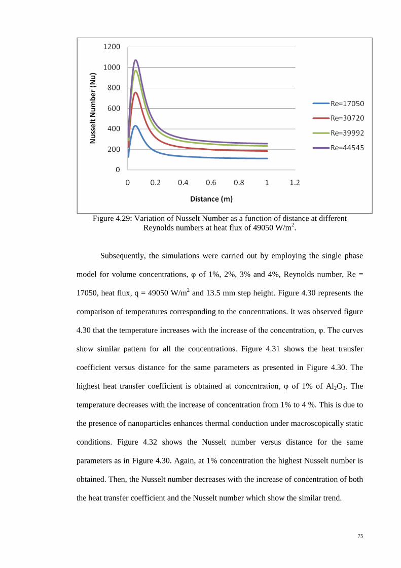
75

Figure 4.29: Variation of Nusselt Number as a function of distance at different

Reynolds numbers at heat flux of 49050 W/m2.

Subsequently, the simulations were carried out by employing the single phase

model for volume concentrations, φ of 1%, 2%, 3% and 4%, Reynolds number, Re =

17050, heat flux, q = 49050 W/m2 and 13.5 mm step height. Figure 4.30 represents the

comparison of temperatures corresponding to the concentrations. It was observed figure

4.30 that the temperature increases with the increase of the concentration, φ. The curves

show similar pattern for all the concentrations. Figure 4.31 shows the heat transfer

coefficient versus distance for the same parameters as presented in Figure 4.30. The

highest heat transfer coefficient is obtained at concentration, φ of 1% of Al2O3. The

temperature decreases with the increase of concentration from 1% to 4 %. This is due to

the presence of nanoparticles enhances thermal conduction under macroscopically static

conditions. Figure 4.32 shows the Nusselt number versus distance for the same

parameters as in Figure 4.30. Again, at 1% concentration the highest Nusselt number is

obtained. Then, the Nusselt number decreases with the increase of concentration of both

the heat transfer coefficient and the Nusselt number which show the similar trend.

76

Figure 4.30: Temperature variation as a function of versus distance for water Al2O3

nanofluids at different concentrations and at heat flux of 49050W/m2.

Figure 4.31: Graphical representation of Heat Transfer Coefficient as a function of distance for water Al2O3 nanofluids at different concentrations and at heat flux of

49050W/m2.

77

Figure 4.32: Nusselt Number variation with distance for water Al2O3 nanofluids at

different concentrations and at heat flux of 49050W/m2.

Average Nusselt number (Nuavg) as function of Reynolds number along the test

section for different step heights are shown in figure 4.33. The result represents

increase of Nusselt number following the dimensions of different step heights. By

increasing the Reynolds number, higher value of average Nusselt number was obtained.

The increase of step height also induces higher average Nusselt number.

Figure 4.33: Average Nusselt number as a function of Reynolds number at different step

heights.

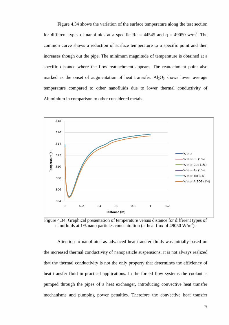
78

Figure 4.34 shows the variation of the surface temperature along the test section

for different types of nanofluids at a specific Re = 44545 and q = 49050 w/m2. The

common curve shows a reduction of surface temperature to a specific point and then

increases though out the pipe. The minimum magnitude of temperature is obtained at a

specific distance where the flow reattachment appears. The reattachment point also

marked as the onset of augmentation of heat transsfer. Al2O3 shows lower average

temperature compared to other nanofluids due to lower thermal conductivity of

Aluminium in comparison to other considered metals.

Figure 4.34: Graphical presentation of temperature versus distance for different types of

nanofluids at 1% nano particles concentration (at heat flux of 49050 W/m2).

Attention to nanofluids as advanced heat transfer fluids was initially based on

the increased thermal conductivity of nanoparticle suspensions. It is not always realized

that the thermal conductivity is not the only property that determines the efficiency of

heat transfer fluid in practical applications. In the forced flow systems the coolant is

pumped through the pipes of a heat exchanger, introducing convective heat transfer

mechanisms and pumping power penalties. Therefore the convective heat transfer

79

coefficient becomes more important than the thermal conductivity value. Evaluation of

cooling efficiency, i.e. ability of the heat transfer fluid to remove heat from the heat

source depends on the flow regime and includes assessment of contributions from

thermal conductivity, viscosity, specific heat, and density of the fluid and can be

estimated from the fluid dynamics equations in assumption of a single phase flow. High

viscosity of nanofluids compared to base fluid increases the power required to pump the

fluid through the system. When the benefit of the increased heat transfer is larger than

the penalty of the increased pumping power, the nanofluid has the potential for

commercial viability. In turbulent flow regime the heat transfer rate (based on the

Dittus-Boelter equation for heating applications) is dependent not only upon the thermal

conductivity (k), but also on the density (ρ), specific heat (cp), viscosity (µ) and flow

velocity (V). Introduction of nanoparticles to the fluid affects all of thermo-physical

properties and should be accounted for in the nanofluid evaluations. Density and

specific heat are proportional to the volume ratio of solid and liquid in the system,

generally with density increasing and specific heat decreasing with addition of solid

nanoparticles to the fluid. The increase in density, specific heat and thermal

conductivity of nanofluids favors the heat transfer coefficient; however the well

described increase in the viscosity of nanoparticle suspensions is not beneficial for heat

transfer. The velocity term also represents the pumping power penalties resulting from

the increased viscosity of nanofluids. It is obvious that nanofluids are multivariable

systems, with each thermo-physical property dependent on several parameters including

nanoparticle material, concentration, size, and shape, properties of the base fluid, and

presence of additives, surfactants, electrolyte strength, and pH. Thus, the challenge in

the development of nanofluids for heat transfer applications is in understanding of how

micro- and macro-scale interactions between the nanoparticles and the fluid affect the

properties of the suspensions.

80

CHAPTER 5: Conclusions

Numerical simulations were conducted for expansion ratios of d/D = 1, 1.16,

1.53 and 1.80. The parameters varied are heat flux, q=719 W/m2, 968 W/m2, 1458

W/m2, and 2098 W/m2 and also Reynolds number, Re=17050, 30720, 39992, and

44545.

The mesh interval size of 6 is suitable for the specific dimension of the pipe as it

is capable of determining heat transfer coefficient and Nusselt number. Mesh interval

size of 6 shows good agreement in achieving surface temperature along the test pipe

with 8.99 % error. Standard k–ԑ model is suitable for the investigation as it offers better

result in calculating the surface temperatures compared to RNG and realizable models.

Standard k–ԑ is able to predict position of reattachment point and surface temperature

more accurately. Thus, the standard k–ԑ model is suitable for investigating turbulent

flow in sudden expansion annular passage in the present case of simple and

axisymmetric geometry.

The increase of flow reduces the surface temperature along the pipe to a

minimum point then increases through the rest of the pipe. The minimum surface

temperature is obtained at flow reattachment point. The position of the minimum

temperature point is dependent on the flow velocity over sudden expansion. Generally,

the local Nusselt number (Nu) increases with the increase of the Reynolds number.

Simulations were conducted for an annular passage with different step heights

and expansion ratios. Generally, the surface temperature along the test pipe may be

81

affected by many variables, such as concentration, heat flux, velocity and the step height

of the test pipe.

Numerically the effect of backward facing step in an annular passage flow

separation on heat transfer for the two dimensional axisymmetric turbulent flow is

studied. Then the influence of variable parameters such as wall heat flux, fluid flow

velocity, separation step height and various fluids on heat transfer characteristic is

determined. The augmentation of heat transfer in the distance of 4 diameters in air and

10 diameters in water after expansion is suggested to increase the performance of heat

exchangers based on the simulation design and parameters.

Heat transfer coefficient of nanofluids increases with increase in the volume

concentration of nanofluids and Reynolds number. Higher temperature operation of the

nanofluids yields higher percentage increase in heat transfer rate. Increase of velocity

and step height causes the surface temperature reduction up to a specific point (lowest

temperature) along the test section and then increases. This lowest temperature

represents the flow reattachment point. The position of this lowest temperature is mainly

a function of step height.

The local heat transfer coefficient (hx) increases with increase of the Reynolds

number for all cases of step heights. In the separation region (recirculation zone) the

local heat transfer coefficient improves until it reaches a maximum value at the

reattachment point. Average Nusselt number decrease with increase of the concentration

of nanofluids due to increase of thermal conductivity of the suspension. Nusselt number

increases with the increase of Reynolds number for all concentrations. Finally, with the

82

advent of computational fluid dynamic software (Fluent), it could provide fair and

agreeable results for the present research.

83

List of Publications and Awards

Academic Journals

1. Numerical Simulation of Heat Transfer to Separation Air Flow in an Annular

Pipe. International Communications in Heat and Mass Transfer. 2012

(Published; ISI-Cited Publication, Q1)

2. Performance investigation of a power augmented vertical axis wind turbine for

urban high-rise application. Renewable Energy. 2013 (Published; ISI-Cited

Publication, Q2)

3. Exhaust Air and Wind Energy Recovery System for Clean Energy Generation,

International Journal of Environmental Sciences and Development. 2011

(Published, ISI-Cited Publication)

Proceedings

1. A Computational Simulation of Heat Transfer to Separation Air Flow in a

Concentric Pipe. International Conference on Applications and Design in

Mechanical Engineering (ICADME). Penang. 27-28 February 2012. (Published;

ISI-Cited Publication)

2. Vertical axis wind turbine with omni-directional-guide-vane for urban high rise

application. International Conference of WREC-Asia & SuDBE2011,

Chongqing, China 28-31 October 2011 (Published, ISI-Cited Publication)

84

3. Exhaust Air and Wind Energy Recovery system for Clean Energy Generation.

Proceedings of International Conference on Environment and Industrial

Innovation (ISI Proceedings). Kuala Lumpur. 4-5 June 2011. (Published,

ISI/SCOPUS Cited Publication)

Award

1. Malaysia Technology Expo Gold Medal award. (Exhaust Air / Wind Energy

Recovery System) 17-19 February 2011, Kuala Lumpur.

85

References

ABBASSI, H. & BEN NASSRALLAH, S. 2007. MHD flow and heat transfer in a backward-facing step. International Communications in Heat and Mass Transfer, 34, 231-237.

ABE, K., KONDOH, T. & NAGANO, Y. 1994. A new turbulence model for predicting fluid flow and heat transfer in separating and reattaching flows—I. Flow field calculations. International Journal of Heat and Mass Transfer, 37, 139-151.

ABE, K., KONDOH, T. & NAGANO, Y. 1995. A new turbulence model for predicting fluid flow and heat transfer in separating and reattaching flows—II. Thermal field calculations. International Journal of Heat and Mass Transfer, 38, 1467-1481.

ABU-MULAWEH, H. I. 2003. A review of research on laminar mixed convection flow over backward- and forward-facing steps. International Journal of Thermal Sciences, 42, 897-909.

ABU-NADA, E. 2008. Application of nanofluids for heat transfer enhancement of separated flows encountered in a backward facing step. International Journal of Heat and Fluid Flow, 29, 242-249.

AHN, J. W., PARK, T. S. & SUNG, H. J. 1997. Application of a near-wall turbulence model to the flows over a step with inclined wall. International Journal of Heat and Fluid Flow, 18, 209-217.

AL-ASWADI, A. A., MOHAMMED, H. A., SHUAIB, N. H. & CAMPO, A. 2010. Laminar forced convection flow over a backward facing step using nanofluids. International Communications in Heat and Mass Transfer, 37, 950-957.

ARMALY, B. F., DURST, F., PEREIRA, J. C. F. & SCHOENUNG, B. 1983a. EXPERIMENTAL AND THEORETICAL INVESTIGATION OF BACKWARD-FACING STEP FLOW. Journal of Fluid Mechanics, 127, 473-496.

ARMALY, B. F., DURST, F., PEREIRA, J. C. F. & SCHÖNUNG, B. 1983b. Experimental and theoretical investigation of backward-facing step flow. Journal of Fluid Mechanics, 127, 473-496.

AUNG, W., BARON, A. & TSOU, F. K. 1985. WALL INDEPENDENCY AND EFFECT OF INITIAL SHEAR-LAYER THICKNESS IN SEPARATED FLOW AND HEAT-TRANSFER. International Journal of Heat and Mass Transfer, 28, 1757-1771.

BARTON, I. E. 1997. Laminar flow over a backward-facing step with a stream of hot particles. International Journal of Heat and Fluid Flow, 18, 400-410.

BIANCO, V., CHIACCHIO, F., MANCA, O. & NARDINI, S. 2009. Numerical investigation of nanofluids forced convection in circular tubes. Applied Thermal Engineering, 29, 3632-3642.

BIANCO, V., MANCA, O. & NARDINI, S. 2011. Numerical investigation on nanofluids turbulent convection heat transfer inside a circular tube. International Journal of Thermal Sciences, 50, 341-349.

BRINKMAN, H. C. 1952. The Viscosity of Concentrated Suspensions and Solutions. Journal of Chemical Physics, 20, 571-581.

BSEBSU, F. M. & BEDE, G. 2002. Theoretical study in single-phase forced-convection heat transfer characteristics for narrow annuli fuel coolant channels. periodica polytechnica ser. Mech. Eng 46, 15–27.

CHEN, C.-K., YEN, T.-S. & YANG, Y.-T. 2006a. Lattice Boltzmann method simulation of backward-facing step on convective heat transfer with field

86

synergy principle. International Journal of Heat and Mass Transfer, 49, 1195-1204.

CHEN, Y. T., NIE, J. H., HSIEH, H. T. & SUN, L. J. 2006b. Three-dimensional convection flow adjacent to inclined backward-facing step. International Journal of Heat and Mass Transfer, 49, 4795-4803.

CHOWDHURY, S. J. & AHMADI, G. 1992. A thermodynamically consistent rate-dependent model for turbulence—part II. Computational results. International Journal of Non-Linear Mechanics, 27, 705-718.

CHUN, K. B. & SUNG, H. J. 1996. Control of turbulent separated flow over a backward-facing step by local forcing. Experiments in Fluids, 21, 417-426.

D.WEN, Y. D. 2004. Experimental investigation into convective heat transfer of nanofluids at the entrance region under laminar flow conditions. Int. J. Heat MassTransfer, 5181-5188.

DAS, S. K., CHOI, S. U. S. & PATEL, H. E. 2006a. Heat Transfer in Nanofluids—A Review. Heat Transfer Engineering, 27, 3-19.

DAS, S. K., CHOI, S. U. S. & PATEL, H. E. 2006b. Heat transfer in nanofluids - A review. Heat Transfer Engineering, 27, 3-19.

DUANGTHONGSUK, W. & WONGWISES, S. 2009. Heat transfer enhancement and pressure drop characteristics of TiO2-water nanofluid in a double-tube counter flow heat exchanger. International Journal of Heat and Mass Transfer, 52, 2059-2067.

EIYAD, A.-N. 2008. Application of nanofluids for heat transfer enhancement of separated flows encountered in a backward facing step. International Journal of Heat and Fluid Flow, 29, 242-249.

FURUICHI, N., HACHIGA, T. & KUMADA, M. 2004. An experimental investigation of a large-scale structure of a two-dimensional backward-facing step by using advanced multi-point LDV. Experiments in Fluids, 36, 274-281.

GOLDSTEIN, R. J., ERIKSEN, V. L., OLSON, R. M. & ECKERT, E. R. G. 1970. Laminar Separation, Reattachment, and Transition of the Flow Over a Downstream-Facing Step. Journal of Basic Engineering, 92, 732-739.

HSU, C.-H. & CHOU, T.-Y. 1997. Unsteady flow of a second-grade fluid past a backward-facing step. International Journal of Non-Linear Mechanics, 32, 947-960.

HWANG, K. S., JANG, S. P. & CHOI, S. U. S. 2009. Flow and convective heat transfer characteristics of water-based Al2O3 nanofluids in fully developed laminar flow regime. International Journal of Heat and Mass Transfer, 52, 193-199.

IWAI, H., NAKABE, K. & SUZUKI, K. 2000. Flow and heat transfer characteristics of backward-facing step laminar flow in a rectangular duct. International Journal of Heat and Mass Transfer, 43, 457-471.

KAKAÇ, S. & PRAMUANJAROENKIJ, A. 2009. Review of convective heat transfer enhancement with nanofluids. International Journal of Heat and Mass Transfer, 52, 3187-3196.

KASAGI, N. & MATSUNAGA, A. 1995. Three-dimensional particle-tracking velocimetry measurement of turbulence statistics and energy budget in a backward-facing step flow. International Journal of Heat and Fluid Flow, 16, 477-485.

KAZI, S. N., DUFFY, G. G. & CHEN, X. D. 2010. Mineral scale formation and mitigation on metals and a polymeric heat exchanger surface. Applied Thermal Engineering, 30, 2236-2242.

KEBLINSKI, P., PHILLPOT, S. R., CHOI, S. U. S. & EASTMAN, J. A. 2002. Mechanisms of heat flow in suspensions of nano-sized particles (nanofluids). International Journal of Heat and Mass Transfer, 45, 855-863.

87

KHANAFER, K., VAFAI, K. & LIGHTSTONE, M. 2003. Buoyancy-driven heat transfer enhancement in a two-dimensional enclosure utilizing nanofluids. International Journal of Heat and Mass Transfer, 46, 3639-3653.

KHOEINI, D., AKHAVAN-BEHABADI, M. A. & SABOONCHI, A. 2012. Experimental study of condensation heat transfer of R-134a flow in corrugated tubes with different inclinations. International Communications in Heat and Mass Transfer, 39, 138-143.

KIM, J.-J. & BAIK, J.-J. 2004. A numerical study of the effects of ambient wind direction on flow and dispersion in urban street canyons using the RNG k–ε turbulence model. Atmospheric Environment, 38, 3039-3048.

KIM, W. S., TALBOT, C., CHUNG, B. J. & JACKSON, J. D. 2002. Variable Property Mixed Convection Heat Transfer to Air Flowing Through a Vertical Passage of Annular Cross Section: Part 1. Chemical Engineering Research and Design, 80, 239-245.

KO, S. 1999. A near-wall reynolds stress model for backward-facing step flows. Journal of Mechanical Science and Technology, 13, 200-210.

KOLACZKOWSKI, S. T., CHAO, R., AWDRY, S. & SMITH, A. 2007. Application of a CFD Code (FLUENT) to Formulate Models of Catalytic Gas Phase Reactions in Porous Catalyst Pellets. Chemical Engineering Research and Design, 85, 1539-1552.

KOUTMOS, P. & MAVRIDIS, C. 1997. A computational investigation of unsteady separated flows. International Journal of Heat and Fluid Flow, 18, 297-306.

KREITH, F. & BOHN, M. S. 2001. Principles of Heat Transfer, Colorado, Cengage Learning.

KUMAR, A. & DHIMAN, A. K. 2012. Effect of a circular cylinder on separated forced convection at a backward-facing step. International Journal of Thermal Sciences, 52, 176-185.

KURTBAŞ, İ. 2008. The effect of different inlet conditions of air in a rectangular channel on convection heat transfer: Turbulence flow. Experimental Thermal and Fluid Science, 33, 140-152.

LAUNDER, B. E. & RODI, W. 1983. THE TURBULENT WALL JET - MEASUREMENTS AND MODELING. Annual Review of Fluid Mechanics, 15, 429-459.

LEE, D., LEE, J., PARK, H. & KIM, M. 2011. Experimental and numerical study of heat transfer downstream of an axisymmetric abrupt expansion and in a cavity of a circular tube. Journal of Mechanical Science and Technology, 25, 395-401.

MISSIRLIS, D., YAKINTHOS, K., PALIKARAS, A., KATHEDER, K. & GOULAS, A. 2005. Experimental and numerical investigation of the flow field through a heat exchanger for aero-engine applications. International Journal of Heat and Fluid Flow, 26, 440-458.

MOHAMMED, H. A., GUNNASEGARAN, P. & SHUAIB, N. H. 2011. Influence of channel shape on the thermal and hydraulic performance of microchannel heat sink. International Communications in Heat and Mass Transfer, 38, 474-480.

MURATA, A. & IWAMOTO, K. 2011. Heat and fluid flow in cylindrical and conical annular flow-passages with through flow and inner-wall rotation. International Journal of Heat and Fluid Flow, 32, 378-391.

MURSHED, S. M. S., LEONG, K. C. & YANG, C. 2008. Thermophysical and electrokinetic properties of nanofluids – A critical review. Applied Thermal Engineering, 28, 2109-2125.

NAIT BOUDA, N., SCHIESTEL, R., AMIELH, M., REY, C. & BENABID, T. 2008. Experimental approach and numerical prediction of a turbulent wall jet over a

88

backward facing step. International Journal of Heat and Fluid Flow, 29, 927-944.

OON, C. S., TOGUN, H., KAZI, S. N., BADARUDIN, A., ZUBIR, M. N. M. & SADEGHINEZHAD, E. 2012. Numerical simulation of heat transfer to separation air flow in an annular pipe. International Communications in Heat and Mass Transfer, 39, 1176-1180.

OTA, T. & KON, N. 1979. Heat transfer in the separated and reattached flow over blunt flat plates —Effects of nose shape. International Journal of Heat and Mass Transfer, 22, 197-206.

PAK, B. C. & CHO, Y. I. 1998. Hydrodynamic and heat transfer study of dispersed fluids with submicron metallic oxide particles. Experimental Heat Transfer, 11, 151-170.

Q.LI, Y. X., PROC. 2002. Convective heat transfer performances of fluids with nano -particles. Int.Heat Transfer Conference,Grenoble,France, 483-488.

R.BENMANSOUR, N. G., C.T.NGUYEN 2009. Developing laminar mixed convection of nanofluids in an inclined tube w ith uniform wall heat flux. Int.J.Num.Meth. Heat Fluid Flow, 19, 146-164.

RAHGOSHAY, M., RANJBAR, A. A. & RAMIAR, A. 2012. Laminar pulsating flow of nanofluids in a circular tube with isothermal wall. International Communications in Heat and Mass Transfer, 39, 463-469.

RAJESH KANNA, P. & MANAB KUMAR, D. 2006. Conjugate heat transfer study of backward-facing step flow – A benchmark problem. International Journal of Heat and Mass Transfer, 49, 3929-3941.

REA, U., MCKRELL, T., HU, L. W. & BUONGIORNO, J. 2009. Laminar convective heat transfer and viscous pressure loss of alumina-water and zirconia-water nanofluids. International Journal of Heat and Mass Transfer, 52, 2042-2048.

ROUIZI, Y., FAVENNEC, Y., VENTURA, J. & PETIT, D. 2009. Numerical model reduction of 2D steady incompressible laminar flows: Application on the flow over a backward-facing step. Journal of Computational Physics, 228, 2239-2255.

S.Z.HERIS, S. G. E., M.N.ESFAHANY, 2006. Exprimental invistegation of oxide nanofluids laminar flow convective heat transfer. Int.Commun.Heat Mass Transfer, 529-535.

TEREKHOV, V. I. & PAKHOMOV, M. A. 2009. Predictions of turbulent flow and heat transfer in gas–droplets flow downstream of a sudden pipe expansion. International Journal of Heat and Mass Transfer, 52, 4711-4721.

TIHON, J., PĚNKAVOVÁ, V., HAVLICA, J. & ŠIMČÍK, M. The transitional backward-facing step flow in a water channel with variable expansion geometry. Experimental Thermal and Fluid Science.

TOGUN, H., SALMAN, Y. K., SULTAN ALJIBORI, H. S. & KAZI, S. N. 2011. An experimental study of heat transfer to turbulent separation fluid flow in an annular passage. International Journal of Heat and Mass Transfer, 54, 766-773.

TOTA, P. V. 2009. Turbulent Flow Over a Backward-Facing Step Using the RNG k-ε Model [Online]. Available: www.flow3d.com/pdfs/tn/FloSci-TN81.pdf [Accessed].

URUBA, V., JONÁŠ, P. & MAZUR, O. 2007. Control of a channel-flow behind a backward-facing step by suction/blowing. International Journal of Heat and Fluid Flow, 28, 665-672.

WASP, E. J., KENNY, J. P. & GANDHI, R. L. 1977. Solid-liquid flow slurry pipeline transportation, Clausthal, Germany, Trans Tech Publications.

89

WEN, D. & DING, Y. 2004. Experimental investigation into convective heat transfer of nanofluids at the entrance region under laminar flow conditions. International Journal of Heat and Mass Transfer, 47, 5181-5188.

WILLIAMS, W., BUONGIORNO, J. & HU, L.-W. 2008. Experimental Investigation of Turbulent Convective Heat Transfer and Pressure Loss of Alumina/Water and Zirconia/Water Nanoparticle Colloids (Nanofluids) in Horizontal Tubes. Journal of Heat Transfer, 130, 042412-7.

WU, T.-H., XU, Z. & JACKSON, J. D. 2002. Mixed Convection Heat Transfer to Water Flowing Through a Vertical Passage of Annular Cross Section: Part 2. Chemical Engineering Research and Design, 80, 246-251.

WYGNANSKI, I., KATZ, Y. & HOREV, E. 1992. On the applicability of various scaling laws to the turbulent wall jet. Journal of Fluid Mechanics, 234, 669-690.

XUAN, Y. & LI, Q. 2003. Investigation on convective heat transfer and flow features of nanofluids. Journal of Heat Transfer, 125, 151-155.

Y.YANG, Z. G. Z., E.A.GRULKE,W.B.ANDERSON,G.WU, 2005. Heat transfer properties of nanoparticle-in-fluid dispersions (nanofluids) in laminar flow. Int.J. Heat Mass Transfer, 48, 1107-1116.

YAKHOT, V., ORSZAG, S.A., THANGAM, S., GATSKI, T.B., SPEZIALE, & C.G. 1992. Development of turbulence models for shearflows by a double expansion technique. Physics of Fluids A4, 1510–1520.

YAMAMOTO, H., SEKI, N. & FUKUSAKO, S. 1979. Forced Convection Heat Transfer on Heated Bottom Surface of a Cavity. Journal of Heat Transfer, 101, 475-479.

YANG, X. D., MA, H. Y. & HUANG, Y. N. 2005. Prediction of homogeneous shear flow and a backward-facing step flow with some linear and non-linear K–ε turbulence models. Communications in Nonlinear Science and Numerical Simulation, 10, 315-328.

YıLMAZ, I. L. & ÖZTOP, H. F. 2006. Turbulence forced convection heat transfer over double forward facing step flow. International Communications in Heat and Mass Transfer, 33, 508-517.

ZEINALI HERIS, S., ETEMAD, S. G. & NASR ESFAHANY, M. 2006. Experimental investigation of oxide nanofluids laminar flow convective heat transfer. International Communications in Heat and Mass Transfer, 33, 529-535.

ZEINALI HERIS, S., NASR ESFAHANY, M. & ETEMAD, S. G. 2007. Experimental investigation of convective heat transfer of Al2O3/water nanofluid in circular tube. International Journal of Heat and Fluid Flow, 28, 203-210.

ZHANG, Z., & KLEINSTREUER, C. 2003. Low-Reynolds-Number Turbulent Flows in Locally Constricted Conduits : A Comparison Study Introduction. AIAA Journal, 41(5), 831-840.

90

Appendices

Temperature (K)

D/x Re=17050 (Exp.) Re=17050 Re=30720 Re=39992 Re=44545

0.196721 383 398.625 361.007 349.036 344.587 0.393443 365 374.627 345.82 336.721 333.349 0.590164 362.1 364.896 339.677 331.743 328.809 0.786885 360.4 358.484 335.631 328.467 325.821 0.983607 359.5 354.071 332.862 326.23 323.783 1.180328 351.366 331.109 324.798 322.473 1.377049 359.1 350.404 330.392 324.185 321.904 1.57377 358 350.666 330.459 324.211 321.918 1.770492 351.665 330.999 324.621 322.284 1.967213 363.1 353.118 331.82 325.258 322.856 2.163934 354.926 332.854 326.064 323.583 2.360656 357.036 334.076 327.022 324.447 2.557377 369.5 359.36 335.457 328.116 325.434 2.754098 361.772 336.911 329.274 326.48 2.95082 364.202 338.376 330.441 327.538 3.147541 366.638 339.846 331.611 328.599 3.344262 373.1 369.083 341.322 332.787 329.666 3.540984 371.547 342.812 333.975 330.745 3.737705 374.025 344.314 335.174 331.833 3.934426 376.507 345.821 336.377 332.925 4.131148 378.98 347.321 337.576 334.014 4.327869 381.43 348.809 338.764 335.092 4.52459 386.3 383.85 350.277 339.938 336.158 4.721311 386.233 351.725 341.095 337.209 4.918033 388.577 353.149 342.233 338.243 5.114754 390.882 354.552 343.354 339.26 5.311475 393.147 355.933 344.457 340.262 5.508197 395.376 357.294 345.544 341.249 5.704918 397.568 358.636 346.616 342.223 5.901639 395.1 399.725 359.961 347.676 343.185 6.098361 401.849 361.27 348.723 344.136 6.295082 403.939 362.564 349.76 345.078 6.491803 405.997 363.843 350.786 346.01 6.688525 408.022 365.107 351.802 346.934 6.885246 410.014 366.357 352.807 347.849 7.081967 411.974 367.591 353.803 348.754 7.278689 398.5 413.899 368.811 354.788 349.651

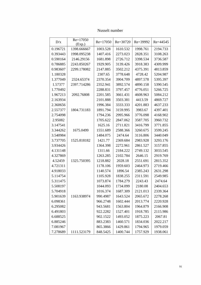
91

Nusselt number

D/x Re=17050 (Exp.) Re=17050 Re=30720 Re=39992 Re=44545

0.196721 1398.666667 1003.528 1610.532 1998.761 2194.733 0.393443 1998.095238 1407.416 2273.023 2828.351 3108.263 0.590164 2146.29156 1681.898 2726.712 3398.534 3736.587 0.786885 2243.850267 1929.905 3139.426 3918.383 4309.999 0.983607 2299.178082 2147.885 3502.212 4375.391 4813.859 1.180328 2307.65 3778.648 4728.42 5204.987 1.377049 2324.65374 2370.354 3904.709 4897.578 5395.397 1.57377 2397.714286 2352.941 3892.574 4890.158 5390.545

1.770492 2288.831 3797.457 4776.051 5266.725 1.967213 2092.76808 2201.585 3661.431 4608.963 5084.212 2.163934 2101.888 3503.381 4413.59 4869.727 2.360656 1996.384 3333.333 4201.883 4637.233 2.557377 1804.731183 1891.794 3159.995 3983.67 4397.401 2.754098 1794.236 2995.966 3776.098 4168.902 2.95082 1705.622 2847.062 3587.705 3960.732

3.147541 1625.16 2711.821 3416.799 3771.855 3.344262 1675.0499 1551.689 2588.366 3260.675 3599.245 3.540984 1484.075 2474.64 3116.806 3440.049 3.737705 1525.818182 1421.77 2369.684 2983.928 3293.176 3.934426 1364.398 2272.961 2861.527 3157.855 4.131148 1311.66 2184.222 2749.132 3033.545 4.327869 1263.285 2102.784 2646.15 2919.769 4.52459 1325.750395 1218.882 2028.18 2551.691 2815.352

4.721311 1178.106 1959.603 2464.973 2719.466 4.918033 1140.574 1896.54 2385.243 2631.298 5.114754 1105.928 1838.255 2311.591 2549.985 5.311475 1073.874 1784.279 2243.43 2474.64 5.508197 1044.093 1734.099 2180.08 2404.653 5.704918 1016.374 1687.309 2121.013 2339.364 5.901639 1163.938974 990.4987 1643.524 2065.672 2278.268 6.098361 966.2748 1602.444 2013.774 2220.928 6.295082 943.5681 1563.804 1964.879 2166.908 6.491803 922.2282 1527.401 1918.785 2115.986 6.688525 902.1522 1493.052 1875.223 2067.81 6.885246 883.2383 1460.571 1834.036 2022.217 7.081967 865.3866 1429.861 1794.965 1979.059 7.278689 1111.523179 848.5425 1400.744 1757.929 1938.061

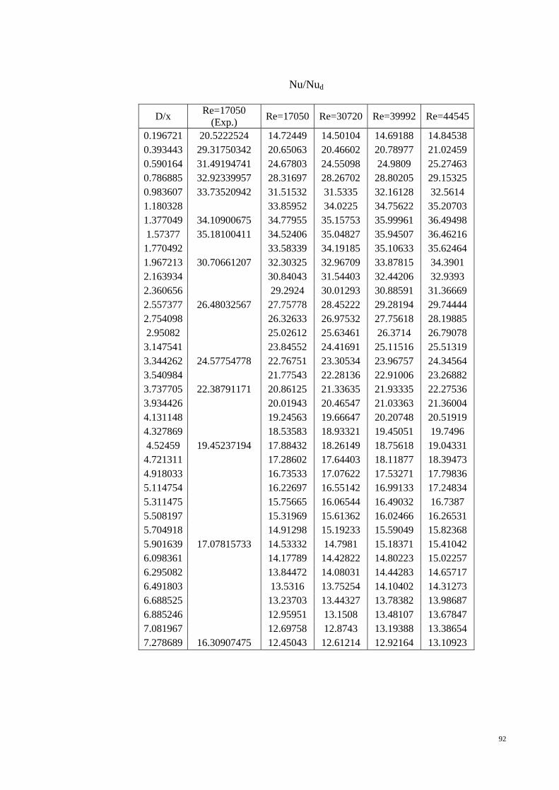
92

Nu/Nud

D/x Re=17050 (Exp.) Re=17050 Re=30720 Re=39992 Re=44545

0.196721 20.5222524 14.72449 14.50104 14.69188 14.84538 0.393443 29.31750342 20.65063 20.46602 20.78977 21.02459 0.590164 31.49194741 24.67803 24.55098 24.9809 25.27463 0.786885 32.92339957 28.31697 28.26702 28.80205 29.15325 0.983607 33.73520942 31.51532 31.5335 32.16128 32.5614 1.180328 33.85952 34.0225 34.75622 35.20703 1.377049 34.10900675 34.77955 35.15753 35.99961 36.49498 1.57377 35.18100411 34.52406 35.04827 35.94507 36.46216 1.770492 33.58339 34.19185 35.10633 35.62464 1.967213 30.70661207 32.30325 32.96709 33.87815 34.3901 2.163934 30.84043 31.54403 32.44206 32.9393 2.360656 29.2924 30.01293 30.88591 31.36669 2.557377 26.48032567 27.75778 28.45222 29.28194 29.74444 2.754098 26.32633 26.97532 27.75618 28.19885 2.95082 25.02612 25.63461 26.3714 26.79078 3.147541 23.84552 24.41691 25.11516 25.51319 3.344262 24.57754778 22.76751 23.30534 23.96757 24.34564 3.540984 21.77543 22.28136 22.91006 23.26882 3.737705 22.38791171 20.86125 21.33635 21.93335 22.27536 3.934426 20.01943 20.46547 21.03363 21.36004 4.131148 19.24563 19.66647 20.20748 20.51919 4.327869 18.53583 18.93321 19.45051 19.7496 4.52459 19.45237194 17.88432 18.26149 18.75618 19.04331 4.721311 17.28602 17.64403 18.11877 18.39473 4.918033 16.73533 17.07622 17.53271 17.79836 5.114754 16.22697 16.55142 16.99133 17.24834 5.311475 15.75665 16.06544 16.49032 16.7387 5.508197 15.31969 15.61362 16.02466 16.26531 5.704918 14.91298 15.19233 15.59049 15.82368 5.901639 17.07815733 14.53332 14.7981 15.18371 15.41042 6.098361 14.17789 14.42822 14.80223 15.02257 6.295082 13.84472 14.08031 14.44283 14.65717 6.491803 13.5316 13.75254 14.10402 14.31273 6.688525 13.23703 13.44327 13.78382 13.98687 6.885246 12.95951 13.1508 13.48107 13.67847 7.081967 12.69758 12.8743 13.19388 13.38654 7.278689 16.30907475 12.45043 12.61214 12.92164 13.10923

93

Cold water Tank Material: Perspex Capacity: (100L)

Water loop Type: stainless steel Diameter: 25mm Overall length: 4.5m

DC power supply Power: 10kW Length: 1m

Chiller

Backward Facing Step Test Rig

Pump Type: centrifugal/stainless steel Power: 1.5 kW Maximum Flow rate: 500l/min Max Velocity: 8m/s

Cooling coil Material: Cooper tube Diameter: 5mm

Cooling unit: 5kW

Magnetic Flowmeter Max Flow rate: 500l/min Max Pressure:170 kPa (absolute P) Min Pressure:100 (absolute P) Max Temperature : 60oC Diameter: (22mm)

Thermocouple (type k) Temperature resolution: 0.01-0.05oC Tempt range: 30-60 oC

DC motor Maximum speed: 100rpm Variable speed control

0.25m

Scale

Length: 4m

1.5m

Differential Pressure transducer Max DP: 0.4 bar Min DP: 0.01 bar

94

Test section

Electrical wire connection

Thermocouple K type Total number: 60 nos

Test section Diameter: 60 mm Length: 1.0m Material: stainless steel

95

Section length: 10mm Number of thermocouples: 30 Interval between thermocouples: 3mm Type: k Thermocouple Diameter: <0.5mm Thermocouple length: 1m Mounting type: welded with epoxy

Section length: 20mm Number of thermocouples: 20 Interval between thermocouples: 3mm Type: k Thermocouple Diameter: <0.5mm Thermocouple length: 1m Mounting type: welded with epoxy

Section length: 70mm Number of thermocouples: 10 Interval between thermocouples: 3mm Type: k Thermocouple Diameter: <0.5mm Thermocouple length: 1m Mounting type: welded with epoxy

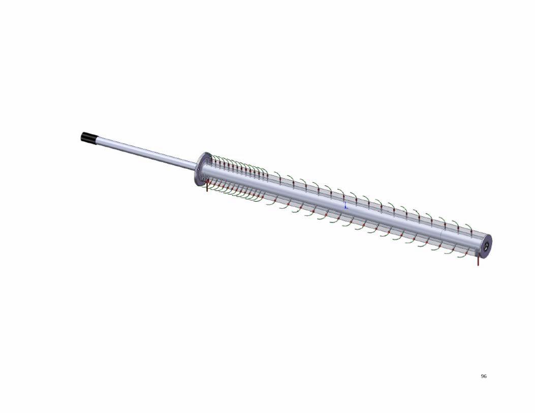
96

97

Backward facing step heat exchanger (2D diagram)

98

Specification

1. Liquid will be pumped to the piping line which will enter the test section and

return back to the tank

2. Tank (100L in size) will be made out of Perspex or non corrosive material

3. Pump power rating (1.5kW)

4. Network pipe is 22mm in diameter

5. All signals from Dp cell, Flowmeter, pump rotation, temperature sensor, and

tyristor will be sent to data logger and processor for further data manipulation

6. Heater power will be controlled by the tyristor which received output signal

from the Data processing unit (DAQ)

7. Pump speed will be controlled by inverter which operate based on flowmeter

signal connected to the DAQ

8. The chiller will receive temperature from the inlet line (T1) instead from the

tank. The refrigerant temperature of the chiller will be automatically adjusted

(by hunting method or any equivalent technique) to meet the line temperature

9. The chiller must have the capability to control the line temperature (T3) on top

of the chiller line temperature (T3)

10. Three temperature sensor are attached to the rod heater which will be sent to the

data logger for averaging

11. This average temperature will serve as the reference for the heater power to

control the amount of power input.