abstract datatypes in pvs - pvs specification...

Abstract Datatypes in PVS

Technical Report CSL-93-9R • December 1993, Substantially RevisedJune 1997

S. OwreN. ShankarOwre,[email protected]

http://pvs.csl.sri.com/

Owre,[email protected]

http://pvs.csl.sri.com/

title

SRI InternationalComputer Science Laboratory • 333 Ravenswood Avenue • Menlo Park CA 94025

The development of the initial version of PVS was funded by internal research funding fromSRI International. More recent versions of PVS have been developed with funding fromARPA, AFOSR, NASA, NSF, and NRL. Support for the preparation of this document camefrom the National Aeronautics and Space Administration Langley Research Center underContract NAS1-18969. This report is a revised and updated version of Technical ReportSRI-CSL-93-09.

Contents

Contents i

1 Introduction 1

2 Lists: A Simple Abstract Datatype 52.1 Positive type occurrence. . . . . . . . . . . . . . . . . . . . . . . . . . . . . 6

3 Binary Trees 93.0.0.1 Definition by cases. . . . . . . . . . . . . . . . . . . . . . . 103.0.0.2 The ord function. . . . . . . . . . . . . . . . . . . . . . . . 113.0.0.3 Extensionality axioms. . . . . . . . . . . . . . . . . . . . . 113.0.0.4 Accessor–constructor axioms. . . . . . . . . . . . . . . . . 123.0.0.5 Eta axiom. . . . . . . . . . . . . . . . . . . . . . . . . . . 123.0.0.6 Structural induction. . . . . . . . . . . . . . . . . . . . . . 123.0.0.7 Definition by recursion. . . . . . . . . . . . . . . . . . . . 133.0.0.8 Subterm relation. . . . . . . . . . . . . . . . . . . . . . . . 153.0.0.9 Well-foundedness. . . . . . . . . . . . . . . . . . . . . . . . 163.0.0.10 The every combinator. . . . . . . . . . . . . . . . . . . . . 163.0.0.11 The some combinator. . . . . . . . . . . . . . . . . . . . . 163.0.0.12 The map combinator. . . . . . . . . . . . . . . . . . . . . . 17

4 Ordered Binary Trees 19

5 In-line and Enumeration Types 23

6 Disjoint Unions 25

7 Mutually Recursive Datatypes 27

8 Lifting Subtyping on Recursive Datatype Parameters 29

i

ii CONTENTS

9 Representations of Recursive Ordinals 31

10 Some Illustrative Proofs about Ordered Binary Trees 3510.1 A Low-level Proof . . . . . . . . . . . . . . . . . . . . . . . . . . . . . . . . 3510.2 A Semi-automated Proof . . . . . . . . . . . . . . . . . . . . . . . . . . . . . 4810.3 Proof Status . . . . . . . . . . . . . . . . . . . . . . . . . . . . . . . . . . . . 54

11 Built-in Datatype Simplifications 55

12 Some Proof Strategies 59

13 Limitations of the PVS Abstract Datatype Mechanism 61

14 Related Work 63

15 Conclusions 6515.0.0.13 Acknowledgements. . . . . . . . . . . . . . . . . . . . . . . 65

Bibliography 67

Chapter 1

Introduction

PVS is a specification and verification environment developed at SRI International.1 Severaldocuments describe the use of PVS [OSRSC98]; this document explains the PVS mecha-nisms for defining and using abstract datatypes.2 It describes a PVS specification for thedata structure of ordered binary trees, defines various operations on this structure, andcontains PVS proofs of some useful properties of these operations. It also describes vari-ous other data structures that can be captured by the PVS abstract datatype mechanism,and documents the built-in capabilities of the PVS proof checker for simplifying abstractdatatype expressions. The exposition does assume some general familiarity with formalmethods but does not require any specific knowledge of PVS.

PVS provides a mechanism for defining abstract datatypes of a certain class. Thisclass includes all of the “tree-like” recursive data structures that are freely generated by anumber of constructor operations.3 For example, the abstract datatype of lists is generatedby the constructors null and cons. The abstract datatype of stacks is generated by theconstructors empty and push. An unordered list or a bag is an example of a data structurethat is not freely generated since two different sequences of insertions of elements into abag can yield equivalent bags. The queue datatype is freely generated but is not consideredrecursive in PVS since the accessor head returning the first element of the queue is not aninverse of the enqueue constructor. This means that the queue datatype must either be

1PVS is freely available and can be obtained via FTP from /pub/pvs/ through the Internet host ftp.

csl.sri.com. The URL http://www.csl.sri.com/pvs.html provides access to PVS-related informationand documents.

2The PVS abstract datatype mechanism is still evolving. Some of the contemplated changes couldinvalidate parts of the description in this report. This report itself updates SRI CSL Technical ReportCSL-93-9 so that it is accurate with respect to the alpha version of PVS 2.1. Future versions of the reportwill be similarly revised to maintain accuracy.

3The abstract datatype mechanism of PVS is partly inspired by the shell principle used in the Boyer-Moore theorem prover [BM79]. Similar mechanisms exist in a number of other specification and programminglanguages.

1

ftp.csl.sri.com

ftp.csl.sri.com

2 Introduction

explicitly axiomatized or implemented using some other datatype such as the list or stackdatatype.

At the semantic level, a recursive datatype introduces a new type constructor that isa solution to a recursive type equation of the form T = τ [T ]. Typically, the recursiveoccurrences of the type name T on the right-hand side must occur only positively (asdefined in Section 2.1) in the type expression τ [T ] and the datatype is the least solution tothe recursion equation. For example, the datatype of lists of element type A is the leastsolution to the type equation T = null+A× T , where + is the disjoint union operationand the × operation returns the Cartesian product. The minimality of lists datatype yieldsa structural induction principle asserting that any list predicate P , if P is closed under thelist datatype operations, i.e., where P (null) and ∀x, l : P (l) ⊃ P (cons(x, l)), then P holdsof all lists. The induction principle also yields a structural recursion theorem asserting thata function that is defined by induction on the structure is total and uniquely defined. Bythe semantic definition of lists, the equality relation on the lists datatype is also the leastequality where the constructor cons can be regarded as a congruence. The minimalityof the equality relation asserts that the constructor cons is an injective operation fromA × list to list. As a consequence of the minimality of equality on the datatype, onecan define accessor functions such as car and cdr on lists constructed using cons, deriveextensionality principles, and define functions by case analysis on the constructor. The PVSdatatype mechanism is used to generate theories introducing the datatype operations forconstructing, recognizing, and accessing datatype expressions, defining structural recursionschemes over datatype expressions, and asserting axioms such as those for extensionalityand induction.

The datatype of lazy lists or streams is also generated by the same recursion schemeusing the constructors null and cons but it is a co-recursive datatype (or a co-datatype)rather than a recursive datatype in that it is the greatest solution to the same recursionequation corresponding to lists. PVS does not yet have a similar mechanism for introducingco-datatypes, and this would be a useful extension to the language. Such a theory ofsequences has been formalized in PVS by Hensel and Jacobs [HJ97] (see also the URL:http://www.cs.kun.nl/~bart/sequences.html).

PVS is a specification language with a set-theoretic semantics. Types are thereforeinterpreted as sets of elements and a function type [A -> B] is interpreted as the set of alltotal maps from the set corresponding to A to that for B. The use of set-theoretic semanticsleads to some important constraints on the form of recursive definitions that can be usedin PVS datatype declarations.

In Section 2, we first present the declaration for the list datatype to convey the syntac-tic restrictions on such datatype declarations. The outcome of such datatype declarations interms of generated theories is explained in detail for the datatype of binary trees in Section 3.In Section 4, the binary tree data structure is used to define ordered binary trees. Section 5shows how enumerated datatypes can be defined as simple forms of PVS datatypes. Sec-

http://www.cs.kun.nl/~bart/sequences.html

Introduction 3

tion 6 shows the definition for disjoint unions. Mutually recursive datatypes are describedin Section 7. Subtyping on recursive datatypes is described in Section 8. In Section 9,datatypes are used to construct effective representations for recursive ordinals which arethen used as lexicographic termination measures for recursive functions. Section 10 showssome proofs about ordered binary trees which use some of the built-in simplifications shownin 11 along with the proof strategies described in Section 12. Some limitations of the PVSdatatype mechanism are described in Section 13, followed by a discussion of related workin Section 14.

4 Introduction

Chapter 2

Lists: A Simple Abstract Datatype

The PVS prelude contains the following declaration of the abstract datatype of lists of agiven element type.

1list[t:TYPE] : DATATYPEBEGINnull: null?cons (car: t, cdr :list) :cons?END list

Here list is declared as a type that is parametric in the type t with two constructorsnull and cons. The constructor null takes no arguments. The predicate recognizer null?holds for exactly those elements of the list datatype that are identical to null. Theconstructor cons takes two arguments where the first is of the type t and the second is alist. The recognizer predicate cons? holds for exactly those elements of the list typethat are constructed using cons, namely, those that are not identical to null. There aretwo accessors corresponding to the two arguments of cons. The accessors car and cdrcan be applied only to lists satisfying the cons? predicate so that car(cons(x, l)) is xand cdr(cons(x, l)) is l. Note that car(null) is not a well typed expression in that itgenerates a invalid proof obligation, a type correctness condition (TCC), that cons?(null)must hold.

The rules on datatype declarations as enforced by the PVS typechecker are:

1. The constructors must be pairwise distinct, i.e., there should be no duplication amongthe constructors.

2. The recognizers must be pairwise distinct, and also distinct from any of the construc-tors and the datatype name itself.

5

6 Lists: A Simple Abstract Datatype

3. There must be at least one non-recursive constructor, that is, one that has no recursiveoccurrences of the datatype in its accessor types.1

4. The recursive occurrences of the datatype name in its definition must be positive asdescribed in Section 2.1.

When the list abstract datatype is typechecked, three theories are generated in thefile list adt.pvs. The first theory, list adt, contains the basic declarations and axiomsformalizing the datatype, including an induction scheme and an extensionality axiom foreach constructor. The second theory, list adt map, defines a map operation that liftsa function of type [s -> t] to a function of type [list[s] -> list[t]]. The thirdtheory, list adt reduce, formalizes a general-purpose recursion operator over the abstractdatatype. These theories are examined in more detail below for the case of binary trees.An important point to note about the generated datatype axioms is that apart from theinduction and extensionality axioms, all the other axioms are automatically applied byPVS proof commands such as assert and beta so that the relevant axioms need never beexplicitly invoked during a proof.

2.1 Positive type occurrence.

For each recursive datatype defined by means of the PVS DATATYPE declaration, the type-checker generates theories, definitions, and axioms similar to those shown above for the caseof binary trees. In general, such a datatype can take individual and type parameters, andis specified in terms of the constructors, and the corresponding recognizers and accessors.The type of the accessor fields can be given recursively in terms of the datatype itself aslong as this recursive occurrence of the type is positive in a certain restricted sense. A typeoccurrence T is positive in a type expression τ iff either

1. τ ≡ T.

2. T occurs positively in a supertype τ ′ of τ .

3. τ ≡ [τ1→τ2] where T occurs positively in τ2. For example, T occurs positively insequence[T] where sequence[T] is defined in the PVS prelude as the function type[nat -> T].

1This is a needless restriction which will be removed in future versions of PVS. It was intended to ensurethat the recursive datatype had a base object. However, it turns out that the restriction does not alwaysguarantee the existence of such a base object such as when the base constructor has an accessor of anempty type. Also datatypes violating this restriction can be well-formed such as a datatype okay with onerecursive constructor mk okay that has one accessor get of type list[okay]. The base object in this case ismk okay(null). When there is no base object, then the datatype is empty.

2.1 Positive type occurrence. 7

4. τ ≡ [τ1, . . . , τn] where T occurs positively in some τi.

5. τ ≡ [# l1 : τ1, . . . , ln : τn #] where T occurs positively in some τi.

6. τ ≡ datatype[τ1, . . . , τn], where datatype is a previously defined datatype and T occurspositively in τi, where τi is a positive parameter of datatype.

The recursive occurrences of the datatype name in its definition must be positive sothat we can assign a set-theoretic interpretation to all types. It is easy to see that violatingthis condition in the recursion leads to contradictions. For example, a datatype T with anaccessor of type [T -> bool] would yield a contradiction since the cardinality of [T ->bool] is that of the power-set of T which by Cantor’s theorem must be strictly greaterthan the cardinality of T. However, we have that distinct accessor elements lead to distinctdatatype elements as well, and hence a contradiction. Similarly, an accessor type of [[T-> bool] -> bool] is also easily ruled out by cardinality considerations even though theoccurrence of T in it is positive in terms of its polarity.

A positive type parameter T in a datatype declaration is one that only occurs positivelyin the type of an accessor. Positive type parameters in datatypes have a special role. Asan example of a nested recursive datatype with recursion on the positive parameters, asearch tree with leaf nodes bearing values of type T can be declared as in 2 . Note that therecursive occurrence of leaftree is as a (positive) parameter to the list datatype.

2leaftree[T : TYPE] : DATATYPEBEGINleaf(val : T) : leaf?node(subs : list[leaftree]): node?END leaftree

Positive datatype parameters are also used to generate the combinators every, some,and map which are described in detail for the datatype of binary trees in Section 3.

8 Lists: A Simple Abstract Datatype

Chapter 3

Binary Trees

A binary tree is a recursive data structure that in the base case is a leaf node, and inthe recursive case consists of a value component, and left and right subtrees that arethemselves binary trees. Binary trees can be formalized in several ways. In most imperativeprogramming languages, they are defined as record structures containing pointers to thesubtrees. They can also be encoded in terms of more primitive recursive data structuressuch as the s-expressions of Lisp. In a declarative specification language, one can formalizebinary trees by enumerating the relevant axioms. One difficulty with this latter approachis the amount of effort involved in correctly identifying all of the relevant axioms. Anotherdifficulty is that it can be tedious to explicitly invoke these axioms during a proof. This is themotivation for providing a concise abstract datatype mechanism in PVS that is integratedwith the theorem prover. With binary trees, the declaration of the datatype is similar tothat for lists above.

3binary_tree[T : TYPE] : DATATYPEBEGINleaf : leaf?node(val : T, left : binary_tree, right : binary_tree) : node?

END binary_tree

The two constructors leaf and node have corresponding recognizers leaf? and node?. Theleaf constructor does not have any accessors. The node constructor has three arguments:the value at the node, the left subtree, and the right subtree. The accessor functions corre-sponding to these three arguments are val, left, and right, respectively. When the abovedatatype declaration is typechecked, the theories binary tree adt, binary tree adt map,and binary tree adt reduce are generated. The first of these has the form:

9

10 Binary Trees

4binary_tree_adt[T: TYPE]: THEORYBEGIN

binary_tree: TYPE

leaf?, node?: [binary_tree -> boolean]

leaf: (leaf?)

node: [[T, binary_tree, binary_tree] -> (node?)]

val: [(node?) -> T]

left: [(node?) -> binary_tree]

right: [(node?) -> binary_tree]

Various axioms and definitions omitted.

END binary_tree_adt

Note that the theory is parametric in the value type T.The first declaration above declares binary tree as a type. The two recognizer predi-

cates on binary trees leaf? and node? are then declared. The constructor leaf is declaredto have type (leaf?) which is the subtype of binary tree constrained by the leaf? pred-icate. The node constructor is declared as a function with domain type [T, binary tree,binary tree] and range type (node?) which is again the subtype of binary tree con-strained by the node? predicate. The three accessors on value (nonleaf) nodes are thendeclared. Each of these accessors takes as its domain the subset of binary trees that areconstructed by means of the node constructor. Note that when binary tree adt is instan-tiated with an empty actual parameter type, the subtype (node?) must be empty sincethere is no value component corresponding to an element of (node?).

The remainder of this section presents the axioms and definitions that are generatedfrom the datatype declaration for binary trees. These axioms and definitions are not meantto be minimal and some of them are in fact redundant.

3.0.0.1 Definition by cases.

The primitive CASES construct is used for definition by cases on the outermost constructorof a a PVS datatype expression. The syntax of the CASES construct is

CASES expression OF selections ENDCASES

Binary Trees 11

where each selection (typically one selection per constructor) is of the form pattern : ex-pression and a pattern is a constructor of arity n applied to n distinct variables. Thereare no explicit axioms characterizing the behavior of CASES. In the case of the binary treedatatype, when w, x, y, and z range over binary trees, a and b range over the parametertype T, u ranges over the range type range, and v ranges over the type [T, binary tree,binary tree -> range], we implicitly assume the two axioms:

CASES leaf OF leaf : u, node(a, y, z) : v(a, y, z) = u

CASES node(b, w, x) OF leaf : u, node(a, y, z) : v(a, y, z) = v(b, w, x)

Note that in the above axioms, the left-hand side occurrences of a, y, and z in v(a, y, z)are bound.

3.0.0.2 The ord function.

The function ord assigns a number to a datatype construction, i.e., a datatype term givensolely in terms of the constructors, according to its outermost constructor. The ord functionis mainly used to enumerate the elements of an enumerated type (see Section 5). The ordfunction is defined using CASES in 5 .

5ord(x: binary_tree): upto(1) =CASES x OF leaf: 0, node(node1_var, node2_var, node3_var): 1 ENDCASES

Thus ord(leaf) is 0, whereas ord(node(x, A, B)) is 1.

3.0.0.3 Extensionality axioms.

An extensionality axiom is generated corresponding to each constructor. The one for theleaf terms essentially asserts that leaf is the unique term of type (leaf?).

6binary_tree_leaf_extensionality: AXIOM(FORALL (leaf?_var: (leaf?), leaf?_var2: (leaf?)):

leaf?_var = leaf?_var2);

For the node constructor, the extensionality axiom is:

7binary_tree_node_extensionality: AXIOM(FORALL (node?_var: (node?)),

(node?_var2: (node?)):val(node?_var) = val(node?_var2)AND left(node?_var) = left(node?_var2)AND right(node?_var) = right(node?_var2)

IMPLIES node?_var = node?_var2)

In other words, any two value nodes that agree on all the accessors are equal.

12 Binary Trees

3.0.0.4 Accessor–constructor axioms.

Each accessor–constructor pair generates an axiom indicating the effect of applying theaccessor to an expression constructed using the constructor. For example, the axiom corre-sponding to val and node has the form:

8binary_tree_val_node: AXIOM(FORALL (node1_var: T), (node2_var: binary_tree),

(node3_var: binary_tree):val(node(node1_var, node2_var, node3_var)) = node1_var)

We do not need an explicit axiom asserting that the recognizers leaf? and node? hold ofdisjoint subsets of the type of binary trees. This property can be derived from the ordfunction and the semantics of the CASES construct described above.

3.0.0.5 Eta axiom.

The eta rule is a useful corollary to the extensionality axiom above and the accessor–constructor axioms shown above. It is introduced as an axiom in the binary tree adttheory as shown below though it does follow as a lemma from extensionality.1

9binary_tree_node_eta: AXIOM(FORALL (node?_var: (node?)):

node(val(node?_var), left(node?_var), right(node?_var)) = node?_var)

3.0.0.6 Structural induction.

The theory binary tree adt also contains a structural induction scheme and a few recursionschemes. The induction scheme for binary trees is stated as:

10binary_tree_induction: AXIOM(FORALL (p: [binary_tree -> boolean]):

p(leaf)AND(FORALL (node1_var: T), (node2_var: binary_tree),

(node3_var: binary_tree): p(node2_var) AND p(node3_var)IMPLIES p(node(node1_var, node2_var, node3_var)))

IMPLIES (FORALL (binary_tree_var: binary_tree): p(binary_tree_var)))

In other words, to prove a property of all binary trees, it is sufficient to prove in the basecase that the property holds of the binary tree leaf, and that in the induction case, theproperty holds of a binary tree node(v, A, B) assuming (the induction hypothesis) that

1In future versions of PVS, it is intended that these will become lemmas with automatically generatedproofs.

Binary Trees 13

it holds of the subtrees A and B. One simple consequence of the induction axiom is theproperty that all binary trees are either leaf nodes or value nodes. This is also introducedas an axiom in the theory binary tree adt.

11binary_tree_inclusive: AXIOM(FORALL (binary_tree_var: binary_tree):

leaf?(binary_tree_var) OR node?(binary_tree_var))

3.0.0.7 Definition by recursion.

As another consequence of induction, we can demonstrate the existence and uniquenessof functions defined by structural recursion over binary trees. It is, however, convenientto have a more direct means for defining such recursive functions. PVS therefore providesvarious recursion combinators2 which can be used to define recursive functions over datatypeelements. One difficulty with defining a fully general recursion combinator is that it has tobe parametric in the range type of the function being defined. Since PVS only provides suchtype parametricity at the level of theories, the generic recursion combinators are defined ina separate theory binary tree adt reduce which provides the additional type parameter.The recursion combinators for the common cases of functions returning natural numbersand sub-ε0 ordinals (see Section 9) are defined in the theory binary tree adt itself.

The recursion combinator used for defining recursive functions over binary trees thatreturn natural number values, is shown below. The idea is that we want to define a functionf by the following recursion over binary trees:

f(leaf) = a

f(node(v, A, B)) = g(v, f(A), f(B))

We define such an f by taking a and g as arguments to the function reduce nat. Note theuse of the CASES construct to define a pattern-matching case split over a datatype valuethat in this case is a binary tree.

2A combinator is a lambda expression without any free variables, but the term can also be applied to anoperation that can be used as a building block for other operations.

14 Binary Trees

12reduce_nat(leaf?_fun: nat, node?_fun: [[T, nat, nat] -> nat]):[binary_tree -> nat] =

LAMBDA (binary_tree_adtvar: binary_tree):CASES binary_tree_adtvar OFleaf: leaf?_fun,node(node1_var, node2_var, node3_var):

node?_fun(node1_var,reduce_nat(leaf?_fun,

node?_fun)(node2_var),

reduce_nat(leaf?_fun,node?_fun)

(node3_var))ENDCASES;

The reduce nat recursion combinator is useful for defining a “size” function as shownin 22 but has the weakness that node? fun only has access to the val field of the node.The theory binary tree adt also contains a variant REDUCE nat where the leaf? fun isa function and the node? fun function takes an additional argument. The definition isomitted here since a more generic version of this recursion combinator is described below.

A generic version of the structural recursion combinator on binary trees is defined inbinary tree adt reduce where the type nat in the definition of reduce nat has beengeneralized to an arbitrary parameter type range.

13binary_tree_adt_reduce[T: TYPE, range: TYPE]: THEORYBEGIN

IMPORTING binary_tree_adt[T]

reduce(leaf?_fun: range, node?_fun: [[T, range, range] -> range]):[binary_tree[T] -> range] =

LAMBDA (binary_tree_var: binary_tree[T]):CASES binary_tree_var OFleaf: leaf?_fun,node(node1_var, node2_var, node3_var):

node?_fun(node1_var,reduce(leaf?_fun,

node?_fun)(node2_var),reduce(leaf?_fun,

node?_fun)(node3_var))ENDCASES

14

END binary_tree_adt_reduce

Binary Trees 15

The theory binary tree adt reduce also contains the more flexible recursion combi-nator REDUCE where the leaf? fun and node? fun functions take binary tree var as anargument.

14REDUCE(leaf?_fun: [binary_tree[T] -> range], node?_fun:[[T, range, range, binary_tree[T]] -> range]):

[binary_tree[T] -> range] =LAMBDA (binary_tree_var: binary_tree[T]):CASES binary_tree_var OFleaf: leaf?_fun(binary_tree_var),node(node1_var, node2_var, node3_var):

node?_fun(node1_var,REDUCE(leaf?_fun,

node?_fun)(node2_var),REDUCE(leaf?_fun,

node?_fun)(node3_var),binary_tree_var)

ENDCASES

PVS 2 introduced certain extensions to the datatype mechanism that were absent inPVS 1. These include a primitive subterm relation, the some, every, and map combinators,and recursion through parameters of previously defined datatypes.

3.0.0.8 Subterm relation.

The primitive subterm relation is defined on datatype objects and checks whether one objectoccurs as a (not necessarily proper) subterm of another object. This relation is defined assubterm.

15subterm(x: binary_tree, y: binary_tree): boolean =x = yOR CASES y OF

leaf: FALSE,node(node1_var, node2_var, node3_var):

subterm(x, node2_var) OR subterm(x, node3_var)ENDCASES

The proper subterm relation is defined by <<. The proper subterm relation is useful as awell-founded termination relation that can be given along with the measure for a recursivelydefined function.

16 Binary Trees

16<<(x: binary_tree, y: binary_tree): boolean =CASES y OFleaf: FALSE,node(node1_var, node2_var, node3_var):

(x = node2_var OR x << node2_var)OR x = node3_var OR x << node3_var

ENDCASES

3.0.0.9 Well-foundedness.

The next axiom asserts that datatype objects are well-founded with respect to the propersubterm relation. The induction axiom binary tree induction can be derived as a con-sequence of the axiom binary tree well founded and the well-founded induction lemmawf induction in the prelude.

17binary_tree_well_founded: AXIOM well_founded?[binary_tree](<<);

3.0.0.10 The every combinator.

The PVS typechecker generates the combinators every and some corresponding to the pos-itive parameters of a datatype. For example, every checks if all values of this parametertype in an instance of the datatype satisfy a given predicate on the parameter type. Fur-thermore, if all the type parameters of a datatype are positive, then a map combinator isalso generated.

The every combinator in the theory binary tree adt takes a predicate p on the positivetype parameter T, and checks that every occurrence of an object of the type parameter in abinary tree satisfies the predicate. The binary tree adt theory also contains a non-curriedvariant of every that is written as every(p, a) instead of every(p)(a).

18every(p: PRED[T])(a: binary_tree): boolean =CASES a OFleaf: TRUE,node(node1_var, node2_var, node3_var):

p(node1_var)AND every(p)(node2_var) AND every(p)(node3_var)

ENDCASES

3.0.0.11 The some combinator.

The some combinator is the dual to every and checks that some occurrence of a value oftype T in the binary tree satisfies the given predicate.3

3For operations like some and every, PVS allows a notational convenience where (some! x: p(x)) isshorthand for some(lambda x: p(x)).

Binary Trees 17

19some(p: PRED[T])(a: binary_tree): boolean =CASES a OFleaf: FALSE,node(node1_var, node2_var, node3_var):

p(node1_var) OR some(p)(node2_var) OR some(p)(node3_var)ENDCASES

3.0.0.12 The map combinator.

Finally, when all the type parameters of a datatype definition occur positively in the def-inition, as is the case with binary tree, a theory binary tree adt map is generated thatdefines the curried and non-curried versions of the map combinator. In addition to theparameter T, binary tree adt map takes a range type parameter T1. The map combinatorapplies a function f from T to T1 to every value of type T in a given binary tree[T] toreturn a result of type binary tree[T1]. We omit the definition of the non-curried variantof map.

20binary_tree_adt_map[T: TYPE, T1: TYPE]: THEORYBEGIN

IMPORTING binary_tree_adt

map(f: [T -> T1])(a: binary_tree[T]): binary_tree[T1] =CASES a OFleaf: leaf[T1],node(node1_var, node2_var, node3_var):

node[T1](f(node1_var),map(f)(node2_var), map(f)(node3_var))

ENDCASES

END binary_tree_adt_map

In summary, the datatype mechanism accepts parametric recursive type definitions interms of constructors, accessors, and recognizers. The recursive occurrences of the datatypemust be positive. The typechecker generates recognizer subtypes, accessor-constructor ax-ioms, extensionality axioms, a structural induction scheme, a subterm ordering relation,and various recursion combinators. With respect to positively occurring type parameters,the typechecker generates the some and every combinators. When all type parameters arepositive, the typechecker also generates a map combinator. We next examine the use of theabove theories formalizing binary trees in the definition of ordered binary trees.

18 Binary Trees

Chapter 4

Ordered Binary Trees

In ordered binary trees, the values in the nodes are ordered relative to each other: the valueat a node is no less than any of the values in the left subtree, and no greater than any of thevalues in the right subtree. Such a data structure has many obvious uses since the valuesare maintained in sorted form and the average time for looking up a value or inserting anew value is logarithmic in the number of nodes.

The PVS specification of ordered binary trees is given in the theory obt below. It isworth noting the use of theory parameters in this specification. The body of the theory obthas been elided from the specification displayed below.

21obt [T : TYPE, <= : (total_order?[T])] : THEORYBEGINIMPORTING binary_tree[T]

A, B, C: VAR binary_treex, y, z: VAR Tpp: VAR pred[T]i, j, k: VAR nat

definitions and lemmas shown below in~ 22 to~ 28

END obt

The theory obt takes the type T of the values kept in the binary tree as its first parameter.Its second parameter is the total ordering used to order the binary tree. This parameter,represented as <=, has the type (total order?[T]) consisting of those binary relations onT that are total orderings, that is, those that are reflexive, transitive, antisymmetric, andlinear. Note that the type of the second parameter to this theory depends on the firstparameter T.

19

20 Ordered Binary Trees

We can now use the every combinator to define when a binary tree is ordered relativeto the theory parameter <=. This notion is captured by the predicate ordered? on binarytrees. Since ordered? will be defined by a direct recursion, its definition will need a measurethat demonstrates the termination of the recursion. In the definition of size below, therecursion combinator reduce nat is used to count the number of value nodes in a givenbinary tree. This function is defined to return 0 when given a leaf, and to increment thesum of the sizes of the left and right subtrees by 1 when given a node.

22size(A) : nat =reduce_nat(0, (LAMBDA x, i, j: i + j + 1))(A)

The recursive definition of ordered? shown below returns TRUE in the base case sincea leaf node is clearly an ordered tree by itself. In the recursive case, the definition ensuresthat the left and right subtrees of the given tree A are themselves ordered. It also usesevery to check that all the values in the left subtree are no greater than the value val(A)at A, and the values in the right subtree are no less than the value at A.

The measure size is used to demonstrate the termination of the recursion displayed byordered?. The proper subterm relation shown in 16 could also be used as a well-foundedrelation in establishing the termination of ordered? by writing MEASURE A BY << (see 34 )in place of MEASURE size.

23ordered?(A) : RECURSIVE bool =(IF node?(A) THEN (every((LAMBDA y: y<=val(A)), left(A)) AND

every((LAMBDA y: val(A)<=y), right(A)) ANDordered?(left(A)) ANDordered?(right(A)))

ELSE TRUE ENDIF)MEASURE size

When the above definition is typechecked, two proof obligations (TCCs) are generatedcorresponding to the termination requirements for the two recursive calls. The first onerequires that the size of the left subtree of a binary tree A must be smaller than the sizeof A. The second proof obligation requires that the size of the right subtree of A mustbe smaller than the size of A. Note how the governing IF-THEN-ELSE condition and thepreceding conjuncts are included as antecedents in the proof obligations below.

Ordered Binary Trees 21

24ordered?_TCC1: OBLIGATION(FORALL (A):

node?(A)AND every((LAMBDA y: y <= val(A)), left(A))AND every((LAMBDA y: val(A) <= y), right(A))

IMPLIES size(left(A)) < size(A));

ordered?_TCC2: OBLIGATION(FORALL (v: [binary_tree[T] -> bool], A):

node?(A)AND every((LAMBDA y: y <= val(A)), left(A))AND every((LAMBDA y: val(A) <= y), right(A)) AND v(left(A))

IMPLIES size(right(A)) < size(A));

The PVS Emacs command M-x tc typechecks a file in PVS. The PVS Emacs command M-xtcp can be used to both typecheck the file and attempt to prove the resulting TCCs usingthe existing proof (if there is one) or a built-in strategy according to the source of the TCC(subtype, termination, existence, assuming, etc.). As it turns out, the termination-tccstrategy automatically proves both ordered? TCC1 and ordered? TCC2.

The next definition in the obt theory is that of the insert operation. The terminsert(x, A) returns that binary tree obtained by inserting the value x at the appro-priate position in the binary tree A. The insert operation is also defined by recursion butemploys the CASES construct instead of the IF-THEN-ELSE conditional. In the base case,when the argument A matches the term leaf, the binary tree containing the single value xis returned as the result. In the recursion case, the argument A has the form node(y, B,C), and if x is at most y according to the given total ordering on the type T, then we recon-struct the node with value y, left subtree insert(x, B), and right subtree C. Otherwise,we reconstruct the node with value y, left subtree B, and right subtree insert(x, C).

25insert(x, A): RECURSIVE binary_tree[T] =(CASES A OF

leaf: node(x, leaf, leaf),node(y, B, C): (IF x<=y THEN node(y, insert(x, B), C)

ELSE node(y, B, insert(x, C))ENDIF)

ENDCASES)MEASURE size(A)

When the above definition is typechecked, two termination proof obligations aregenerated corresponding to the two recursive invocations of insert. Both proof obli-gations insert TCC1 and insert TCC2 are automatically discharged by the defaulttermination-tcc strategy.

22 Ordered Binary Trees

26insert_TCC1: OBLIGATION(FORALL (B: binary_tree[T], C: binary_tree[T], y: T, A, x):

A = node(y, B, C) AND x <= y IMPLIES size(B) < size(A));

insert_TCC2: OBLIGATION(FORALL (B: binary_tree[T], C: binary_tree[T], y: T, A, x):

A = node(y, B, C) AND NOT x <= y IMPLIES size(C) < size(A))

The following lemma states an interesting property of insert. Its proof requires theuse of induction over binary trees. It asserts that if every value in the tree A has propertypp, and the value x also has property pp, then every value in the result of inserting x intoA has property pp.

27ordered?_insert_step: LEMMApp(x) AND every(pp, A) IMPLIES every(pp, insert(x, A))

The theorem ordered? insert asserts the important property of insert that it returnsan ordered binary tree when given an ordered binary tree.

28ordered?_insert: THEOREMordered?(A) IMPLIES ordered?(insert(x, A))

We examine some proofs of this theorem in Section 10.

Chapter 5

In-line and Enumeration Types

The example of binary trees illustrated how abstract datatypes can be declared as theories(that are automatically expanded) within PVS. Abstract datatypes can be declared withinother theories as long as they do not employ any parameters. Note that PVS has typeparameterization only at the theory level and not at the declaration level. For example,the type of combinators constructed out of the K and S combinators is captured by thefollowing declaration that can occur at the declaration level within a theory. The axiomsgenerated by the DATATYPE declaration can be viewed using the PVS Emacs command M-xppe.

29combinators : THEORYBEGINcombinators: DATATYPE

BEGINK: K?S: S?app(operator, operand: combinators): app?

END combinators

x, y, z: VAR combinators

reduces_to: PRED[[combinators, combinators]]

K: AXIOM reduces_to(app(app(K, x), y), x)S: AXIOM reduces_to(app(app(app(S, x), y), z), app(app(x, z), app(y, z)))

END combinators

The most frequently used such in-line abstract datatypes are enumeration types. Forexample, the type of colors consisting of red, white, and blue can given by the followingin-line datatype declaration.

23

24 In-line and Enumeration Types

30colors: DATATYPEBEGINred: red?white: white?blue: blue?

END colors

The above declaration is a rather verbose way of defining the type of colors. PVS pro-vides an abbreviation mechanism that allows the above declaration to be expressed moresuccinctly as shown below.

31colors: TYPE = red, white, blue

All of the axiomatized properties of such enumeration types are built into the PVS proofchecker as shown in the previous section so that no axioms about enumeration types needever be explicitly used.

Chapter 6

Disjoint Unions

The type constructor for the disjoint union of two types is popular enough to be included inseveral languages. The disjoint union of two sets A and B is a set in which each element istagged according to whether it is from A or from B. It is easy to see that the type analogueof the disjoint union operation can be defined using the DATATYPE mechanism of PVS asshown below:

32disj_union[A, B: TYPE] : DATATYPEBEGIN

inl(left : A): inl?inr(right : B): inr?

END disj_union

The type disj union[nat, bool] then includes values such as inl(1) and inr(TRUE).Rushby [Rus95] presents a toy compiler verification exercise [WW93] in PVS and

presents an extensive discussion of the use of disjoint unions in PVS specifications andproofs.

25

26 Disjoint Unions

Chapter 7

Mutually Recursive Datatypes

Mutually recursive datatypes arise quite frequently in programming and specification. Acommon example is that of a language definition where type expressions contain terms andvice-versa. Mutually recursive type definitions are not directly admissible using the PVSdatatype mechanism. But most typical mutual recursive types can, in fact, be defined as asingle datatype in PVS with subtypes that group together classes of constructors. PVS 2 hasbeen extended to admit such datatypes with sub-datatypes. The example below describesthe class of arithmetic expressions that include numbers, sums, and conditional expressionsclassified by the sub-datatype term, where the test component of a conditional expressionis a boolean expression classified by the subdatatype expr. Thus sub-datatypes are a wayof collecting together groups of constructors of a datatype that form one part of a mutuallyrecursive datatype definition. In the example below, boolean expressions are defined asequalities between arithmetic expressions, and conditional arithmetic expressions containboolean subexpressions, so that arithmetic and boolean expressions are mutually recursive.

33arith: DATATYPE WITH SUBTYPES expr, termBEGINnum(n:int): num? :termsum(t1:term,t2:term): sum? :term

% ...eq(t1: term, t2: term): eq? :exprift(e: expr, t1: term, t2: term): ift? :term

% ...END arith

The only restriction on the use of subdatatypes other than those listed in Section 2 isthat the sub-datatypes should be pairwise distinct and differ from the datatype itself. Inparticular, sub-datatypes need not actually be used in which case they are empty. It ispossible to define mutual recursive types that lead to empty constructor subtypes such as if

27

28 Mutually Recursive Datatypes

the eq constructor in the arith datatype was specified as eq(t1: expr, t2: expr): eq?: expr.

An evaluator for such arithmetic/boolean expressions can be defined as eval whoserange type is a disjoint union of bool and int (according to whether the input expressionis of type expr or term. The function eval is therefore dependently typed to return valuesof type (bool?) on inputs of type expr and values of type (int?) on inputs of type term.

34arith_eval: THEORYBEGINIMPORTING arith

value: DATATYPEBEGINbool(b:bool): bool?int(i:int): int?END value

eval(a: arith): RECURSIVEv: value | IF expr(a) THEN bool?(v) ELSE int?(v) ENDIF =

CASES a OFnum(n): int(n),sum(n1, n2): int(i(eval(n1)) + i(eval(n2))),eq(n1, n2): bool(i(eval(n1)) = i(eval(n2))),ift(e, n1, n2): IF b(eval(e)) THEN eval(n1) ELSE eval(n2) ENDIFENDCASESMEASURE a BY <<

END arith_eval

Chapter 8

Lifting Subtyping on RecursiveDatatype Parameters

The datatype mechanism in PVS 2.0 had the limitation that though the type of nat ofnatural numbers is a subtype of the type int of integers, the type list[nat] of lists overthe natural numbers is not a subtype of the type list[int] of lists over the integers. Thedatatype mechanism in PVS 2.1 has been modified to lift such subtyping over positiveparameters to the corresponding abstract datatypes. In general, given a datatype D with apositive type parameter, we have

D[x: T | p(x)] ≡ d: D[T] | every(p)(d).

While cons[nat] is neither syntactically nor semantically identical to cons[int],constructor applications involving cons[int] and cons[nat] such as cons[nat](0,null[nat]) and cons[int](0, null[int]) are syntactically identical. Also, constructorsthat are declared to have no accessors (e.g., null) are syntactically equal, so null[int] ≡null[real], but null[int] and null[bool] belong to incompatible types.

In general, when a constructor, accessor, or recognizer occurs as an operator of anapplication, the actual parameter is only used for testing compatibility. Note that theactual parameter is not actually ignored. For example, the expression cons[nat](-1,null) is not type correct and generates the unprovable proof obligation -1 > 0.

When multiple parameters are involved, only the positive ones satisfy the subtypingequivalences given above. Thus in the datatype declaration

dt[t1, t2: TYPE, c: t1]: DATATYPEBEGINb: b?c(a1:[t1 -> t2], a2: dt): c?END dt

29

30 Lifting Subtyping on Recursive Datatype Parameters

only t2 occurs positively, so dt[int, nat, 3] is a subtype of dt[int, int, 3], but bearsno relation to dt[nat, nat, 3] or to dt[int, nat, 2].

Chapter 9

Representations of RecursiveOrdinals

Ordinals are needed to provide lexicographic termination measures for recursive functions.The Ackermann function provides a well known example of a doubly recursive functionthat requires a lexicographic measure. Peter’s version [Pet67] of the Ackermann function isdefined in the theory ackermann as ack.

35ackermann: THEORYBEGINi, j, k, m, n: VAR nat

ack(m,n): RECURSIVE nat =(IF m=0 THEN n+1

ELSIF n=0 THEN ack(m-1,1)ELSE ack(m-1, ack(m, n-1))

ENDIF)MEASURE lex2(m, n)

...END ackermann

The lexicographic termination measure for ack is computed by the function lex2 (see 39 )which returns a representation for the ordinal in the lexicographic ordering. The ordinalε0 is the least ordinal x such that x = ωx, and therefore includes 0, 1, . . . , ω, ω + 1, . . . ω +ω, . . . , 3 ∗ ω, . . . , ω2, . . . , ωω, . . . , ω.

.ω

, . . . . The sub-ε0 ordinals can be represented using theCantor normal form which asserts that to any non-zero ordinal α, there are n ordinalsα1, . . . , αn with α1 ≤ . . . ≤ αn < α, such that α = ωα1 + ωα2 + . . . + ωαn . We can makethis representation slightly more compact by adding natural number coefficients so that to

31

32 Representations of Recursive Ordinals

any α, there are ordinals α1, . . . , αn such that α1 ≤ . . . ≤ αn < α, and natural numbersc1, . . . , cn such that α = c1∗ωα1 +c2∗ωα2 +. . .+cn∗ωαn . It is easy to see that a lexicographicmeasure can be given by n ∗ ω0 +m ∗ ω which is just n+m ∗ ω.

We now explain how the sub-ε0 ordinals are defined in the PVS prelude. We start bydefining an ordstruct datatype that represents ordinal-like structures.

36ordstruct: DATATYPEBEGINzero: zero?add(coef: posnat, exp: ordstruct, rest: ordstruct): nonzero?END ordstruct

In intuitive terms, the ordinal represented by zero is 0, and the ordinal repre-sented by add(c, alpha, beta) given by, say ordinal(add(c, alpha, beta)) is c ∗ωordinal (alpha) + ordinal(beta). We can then define an ordering relation on ordstructterms as given by < in 37 . It compares add(i, u, v) against add(j, z, w) by eitherrecursively ensuring u < z, or checking that u is syntactically identical to z and either i <j or i = j and recursively v < w.

37ordinals: THEORYBEGINi, j, k: VAR posnatm, n, o: VAR natu, v, w, x, y, z: VAR ordstructsize: [ordstruct->nat] = reduce[nat](0, (LAMBDA i, m, n: 1 + m+n));

<(x, y): RECURSIVE bool =CASES x OF

zero: NOT zero?(y),add(i, u, v): CASES y OF

zero: FALSE,add(j, z, w): (u<z) OR

(u=z) AND (i<j) OR(u=z) AND (i=j) AND (v<w)

ENDCASESENDCASES

MEASURE size(x);

This is not quite the ordering relation we want since it will obviously only work for normal-ized (and therefore, canonical) representations where the exponent ordinals appear in sorted(decreasing) order. In particular, note that the use of syntactic identity on ordstruct termswill not work unless the terms are in fact canonical representatives. It is easy to define apredicate which identifies an ordstruct term as being in the required Cantor normal formby defining a recursive predicate ordinal? as shown in 38 .

Representations of Recursive Ordinals 33

38>(x, y): bool = y < x;<=(x, y): bool = x < y OR x = y;>=(x, y): bool = y < x OR y = x

ordinal?(x): RECURSIVE bool =CASES x OFzero: TRUE,add(i, u, v): (ordinal?(u) AND ordinal?(v) AND

CASES v OFzero: TRUE,add(k, r, s): r < u

ENDCASES)ENDCASESMEASURE size

ordinal: NONEMPTY_TYPE = (ordinal?)

The definition of ordinal? checks add(i, u, v) to recursively ensure that u and v areordinals, and that in add(i, u, add(k, r, s)), we have r < u. This latter use of theordering relation is acceptable since we have already checked that r and u are proper normalforms. The definition of lex2 is given in 39 . Note that add(n, zero, zero) represents n,add(m, add(1, zero, zero), zero) represents m ∗ ω, and add(m, add(1,zero,zero),add(n,zero, zero)) represents n+m ∗ ω.1

39lex2(m, n): ordinal =(IF m=0

THEN IF n = 0THEN zeroELSE add(n, zero, zero)

ENDIFELSIF n = 0 THEN add(m, add(1,zero,zero),zero)ELSE add(m, add(1,zero,zero), add(n,zero, zero))

ENDIF)

lex2_lt: LEMMAlex2(i, j) < lex2(m, n) =(i < m OR (i = m AND j < n))

Returning to the example of the Ackermann function in 35 , the measure lex2(m, n)generates three termination TCCs corresponding to the three recursive invocations of thefunction.

1The PVS CONVERSION mechanism can be used to gracefully embed the natural numbers into the ordinal

type by converting 0 to zero, and a positive number n to add(n, zero, zero).

34 Representations of Recursive Ordinals

40ack_TCC2: OBLIGATION(FORALL (m, n): NOT m = 0 AND n = 0IMPLIES lex2(m - 1, 1) < lex2(m, n));

ack_TCC5: OBLIGATION(FORALL (m, n):

NOT m = 0 AND NOT n = 0IMPLIES lex2(m, n - 1) < lex2(m, n));

ack_TCC6: OBLIGATION(FORALL (v: [[nat, naturalnumber] -> nat], m, n):

NOT m = 0 AND NOT n = 0IMPLIES lex2(m - 1, v(m, n - 1)) < lex2(m, n));

All three TCCs are proved automatically by the default termination-tcc strategy.

Chapter 10

Some Illustrative Proofs aboutOrdered Binary Trees

We present two proofs of ordered? insert shown in 28 . The second proof exhibits agreater level of automation than the first proof. The first proof illustrates the various low-level datatype related proof commands that are provided by PVS, and the second proofillustrates how these commands can be combined to form more powerful and automaticproof strategies. Strategies are similar to the tactics of the LCF [GMW79] family of proofcheckers.

10.1 A Low-level Proof

When we invoke M-x pr on ordered? insert, the theorem to be proved is displayed inthe *pvs* buffer, and we are prompted for an inference rule by the Rule? prompt. Sincethe proof is by induction, the first step in the proof is the command (induct "A"). Thisindicates that we wish to invoke the induct strategy with A as the induction variable. Theinduction strategy finds the induction axiom corresponding to the datatype of A, instantiatesit suitably, and simplifies it to generate the base and induction cases. We are then presentedthe base case of the proof. (The induction case can be displayed with the PVS Emacscommand M-x siblings.

35

36 Some Illustrative Proofs about Ordered Binary Trees

41ordered?_insert :|-------

1 (FORALL (A: binary_tree[T], x: T):ordered?(A) IMPLIES ordered?(insert(x, A)))

Rule? (induct "A")Inducting on A,this yields 2 subgoals:ordered?_insert.1 :|-------

1 (FORALL (x: T): ordered?(leaf) IMPLIES ordered?(insert(x, leaf)))

In the next step, we replace the universally quantified variable with a Skolem constant andflatten the sequent by simplifying all top-level propositional connectives that are disjunctive(i.e., negations, positive implications and disjunctions, and negative conjunctions).

42Rule? (skosimp)Skolemizing and flattening,this simplifies to:ordered?_insert.1 :-1 ordered?(leaf)|-------

1 ordered?(insert(x!1, leaf))

The obvious step now is to open up the definitions of insert and ordered?. This is doneby two invocations of the expand rule.

43Rule? (expand "insert")Expanding the definition of insert,this simplifies to:ordered?_insert.1 :[-1] ordered?(leaf)|-------

1 ordered?(node(x!1, leaf, leaf))

Rule? (expand "ordered?")Expanding the definition of ordered?,this simplifies to:ordered?_insert.1 :|-------

1 (every((LAMBDA (y: T): y <= x!1), leaf)AND every((LAMBDA (y: T): x!1 <= y), leaf)AND ordered?(leaf) AND ordered?(leaf))

The problem now is that all the occurrences of ordered? are expanded so that the an-tecedent formula ordered?(leaf) reduces to TRUE and vanishes from the sequent. This

10.1 A Low-level Proof 37

formula in its unexpanded form is actually useful since it occurs in the consequent partof the sequent. We could press on and expand ordered? once again or, alternatively, wecould undo this step of the proof and expand ordered? more selectively using the command(expand "ordered?" +).

44Rule? (undo)This will undo the proof to:ordered?_insert.1 :[-1] ordered?(leaf)|-------

1 ordered?(node(x!1, leaf, leaf))Sure? (Y or N): yordered?_insert.1 :[-1] ordered?(leaf)|-------

1 ordered?(node(x!1, leaf, leaf))

Rule? (expand "ordered?" +)Expanding the definition of ordered?,this simplifies to:ordered?_insert.1 :[-1] ordered?(leaf)|-------

1 (every((LAMBDA (y: T): y <= x!1), leaf)AND every((LAMBDA (y: T): x!1 <= y), leaf)AND ordered?(leaf) AND ordered?(leaf))

Now an invocation of assert eliminates the occurrences of the subformula ordered?(leaf)in the consequent since it appears in the antecedent. Expanding every then completes thebase case of the proof without any further work.


45Rule? (assert)Simplifying, rewriting, and recording with decision procedures,this simplifies to:ordered?_insert.1 :[-1] ordered?(leaf)|-------

1 (every((LAMBDA (y: T): y <= x!1), leaf)AND every((LAMBDA (y: T): x!1 <= y), leaf))

Rule? (expand "every")Expanding the definition of every,this simplifies to:ordered?_insert.1 :[-1] ordered?(leaf)|-------

1 TRUEwhich is trivially true.This completes the proof of ordered?_insert.1.

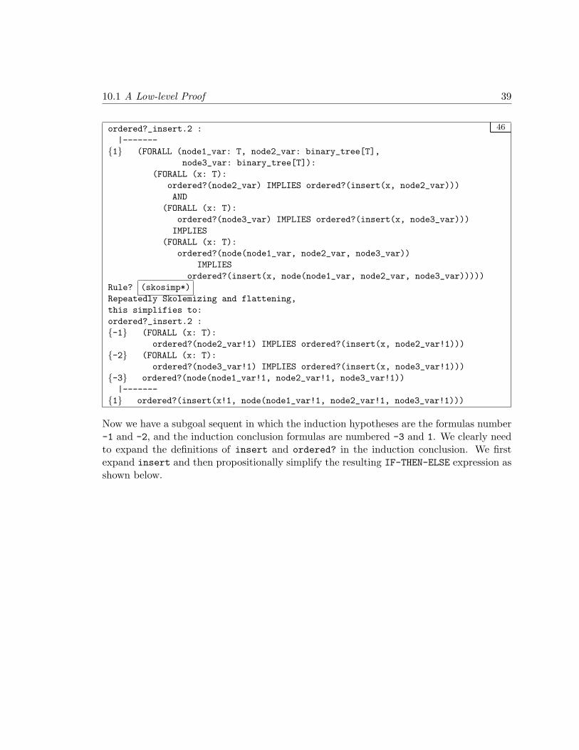
Having completed the base case of the proof, we are left with the induction case. Ourfirst step here is to apply the rule skosimp*. This is a strategy that repeatedly performsa skolem! followed by a flatten until nothing changes, i.e., it is an iterated form of theskosimp command.


46ordered?_insert.2 :|-------

1 (FORALL (node1_var: T, node2_var: binary_tree[T],node3_var: binary_tree[T]):

(FORALL (x: T):ordered?(node2_var) IMPLIES ordered?(insert(x, node2_var)))AND

(FORALL (x: T):ordered?(node3_var) IMPLIES ordered?(insert(x, node3_var)))IMPLIES

(FORALL (x: T):ordered?(node(node1_var, node2_var, node3_var))

IMPLIESordered?(insert(x, node(node1_var, node2_var, node3_var)))))

Rule? (skosimp*)Repeatedly Skolemizing and flattening,this simplifies to:ordered?_insert.2 :-1 (FORALL (x: T):

ordered?(node2_var!1) IMPLIES ordered?(insert(x, node2_var!1)))-2 (FORALL (x: T):

ordered?(node3_var!1) IMPLIES ordered?(insert(x, node3_var!1)))-3 ordered?(node(node1_var!1, node2_var!1, node3_var!1))|-------

1 ordered?(insert(x!1, node(node1_var!1, node2_var!1, node3_var!1)))

Now we have a subgoal sequent in which the induction hypotheses are the formulas number-1 and -2, and the induction conclusion formulas are numbered -3 and 1. We clearly needto expand the definitions of insert and ordered? in the induction conclusion. We firstexpand insert and then propositionally simplify the resulting IF-THEN-ELSE expression asshown below.


47Rule? (expand "insert" +)Expanding the definition of insert,this simplifies to:ordered?_insert.2 :[-1] (FORALL (x: T):

ordered?(node2_var!1) IMPLIES ordered?(insert(x, node2_var!1)))[-2] (FORALL (x: T):

ordered?(node3_var!1) IMPLIES ordered?(insert(x, node3_var!1)))[-3] ordered?(node(node1_var!1, node2_var!1, node3_var!1))|-------

1 IF x!1 <= node1_var!1THEN ordered?(node(node1_var!1, insert(x!1, node2_var!1), node3_var!1))

ELSE ordered?(node(node1_var!1, node2_var!1, insert(x!1, node3_var!1)))ENDIF

Rule? (prop)Applying propositional simplification,this yields 2 subgoals:ordered?_insert.2.1 :-1 x!1 <= node1_var!1[-2] (FORALL (x: T):



1 ordered?(node(node1_var!1, insert(x!1, node2_var!1), node3_var!1))

The propositional simplification step generates two subgoals according to whether the recur-sive invocation of insert is on the left or the right subtree. We first consider the insertioninto the left subtree given by subgoal ordered? insert.2.1. We can instantiate the in-duction hypothesis numbered -2 by applying the inst? command which uses syntacticmatching to find instantiating terms for the universally quantified variable in -2.


48Rule? (inst?)Found substitution:x gets x!1,Instantiating quantified variables,this simplifies to:ordered?_insert.2.1 :[-1] x!1 <= node1_var!1-2 ordered?(node2_var!1) IMPLIES ordered?(insert(x!1, node2_var!1))[-3] (FORALL (x: T):


[1] ordered?(node(node1_var!1, insert(x!1, node2_var!1), node3_var!1))

The next step is to expand the definition of ordered? in the induction conclusion. Notethat the second argument to the expand proof command is a list of the formula numberswhere the expansion is to be performed. It makes the proof considerably less robust if itexplicitly mentions such formula numbers, though this can be unavoidable in some cases.1

49Rule? (expand "ordered?" (-4 1))Expanding the definition of ordered?,this simplifies to:ordered?_insert.2.1 :[-1] x!1 <= node1_var!1[-2] ordered?(node2_var!1) IMPLIES ordered?(insert(x!1, node2_var!1))[-3] (FORALL (x: T):

ordered?(node3_var!1) IMPLIES ordered?(insert(x, node3_var!1)))-4 (every((LAMBDA (y: T): y <= node1_var!1), node2_var!1)

AND every((LAMBDA (y: T): node1_var!1 <= y), node3_var!1)AND ordered?(node2_var!1) AND ordered?(node3_var!1))

|-------1 (every((LAMBDA (y: T): y <= node1_var!1), insert(x!1, node2_var!1))

AND every((LAMBDA (y: T): node1_var!1 <= y), node3_var!1)AND ordered?(insert(x!1, node2_var!1)) AND ordered?(node3_var!1))

Applying propositional simplification prop to the resulting subgoal generates two fur-ther subgoals. The first of these is easily proved by rewriting using the lemmaordered? insert step. Note that this is a conditional rewrite rule and has the formA ⊃ B, where the rewriting given by B can be applied to a matching instance σ(B) onlywhen the corresponding σ(A) (the condition) is provable. The rewrite proof strategy at-tempts to discharge these conditions automatically, and any undischarged conditions aregenerated as subgoals.

1PVS is currently being enhanced to allow labels to be introduced for sequent formulas so that formulaselection in the PVS proof commands can be done with labels as an alternative to formula numbers.


50Rule? (prop)Applying propositional simplification,this simplifies to:ordered?_insert.2.1 :-1 ordered?(insert(x!1, node2_var!1))[-2] x!1 <= node1_var!1[-3] (FORALL (x: T):

ordered?(node3_var!1) IMPLIES ordered?(insert(x, node3_var!1)))-4 every((LAMBDA (y: T): y <= node1_var!1), node2_var!1)-5 every((LAMBDA (y: T): node1_var!1 <= y), node3_var!1)-6 ordered?(node2_var!1)-7 ordered?(node3_var!1)|-------

1 every((LAMBDA (y: T): y <= node1_var!1), insert(x!1, node2_var!1))

Rule? (rewrite "ordered?_insert_step")Found matching substitution:A gets node2_var!1,x gets x!1,pp gets (LAMBDA (y: T): y <= node1_var!1),Rewriting using ordered?_insert_step,This completes the proof of ordered?_insert.2.1.

We have now completed the part of the proof corresponding to the insertion into theleft subtree. Next, we proceed to the case when the insert operation is applied to the rightsubtree. This case is similar to the proof of ordered? insert.2.1.

51ordered?_insert.2.2 :[-1] (FORALL (x: T):



1 x!1 <= node1_var!12 ordered?(node(node1_var!1, node2_var!1, insert(x!1, node3_var!1)))

As in 48 earlier, we apply the step inst?.


52Rule? (inst?)Found substitution:x gets x!1,Instantiating quantified variables,this simplifies to:ordered?_insert.2.2 :-1 ordered?(node2_var!1) IMPLIES ordered?(insert(x!1, node2_var!1))[-2] (FORALL (x: T):


[1] x!1 <= node1_var!1[2] ordered?(node(node1_var!1, node2_var!1, insert(x!1, node3_var!1)))

It however instantiates the formula -1 which is not the appropriate induction hypothesisfor the right branch. To apply the inst? step with greater selectivity, we undo the last stepand supply a further argument to inst? indicating the number of the quantified formulato be instantiated.

53Rule? (inst? -2)Found substitution:x gets x!1,Instantiating quantified variables,this simplifies to:ordered?_insert.2.2 :[-1] (FORALL (x: T):

ordered?(node2_var!1) IMPLIES ordered?(insert(x, node2_var!1)))-2 ordered?(node3_var!1) IMPLIES ordered?(insert(x!1, node3_var!1))[-3] ordered?(node(node1_var!1, node2_var!1, node3_var!1))|-------

[1] x!1 <= node1_var!1[2] ordered?(node(node1_var!1, node2_var!1, insert(x!1, node3_var!1)))

Now, as before, we expand the definition of ordered? in the induction conclusion formulas-3 and 2.


54Rule? (expand "ordered?" (-3 2))Expanding the definition of ordered?,this simplifies to:ordered?_insert.2.2 :[-1] (FORALL (x: T):

ordered?(node2_var!1) IMPLIES ordered?(insert(x, node2_var!1)))[-2] ordered?(node3_var!1) IMPLIES ordered?(insert(x!1, node3_var!1))-3 (every((LAMBDA (y: T): y <= node1_var!1), node2_var!1)


|-------[1] x!1 <= node1_var!12 (every((LAMBDA (y: T): y <= node1_var!1), node2_var!1)

ANDevery((LAMBDA (y: T): node1_var!1 <= y), insert(x!1, node3_var!1))

AND ordered?(node2_var!1) AND ordered?(insert(x!1, node3_var!1)))

Propositional simplification yields a single goal sequent.

55Rule? (prop)Applying propositional simplification,this simplifies to:ordered?_insert.2.2 :-1 ordered?(insert(x!1, node3_var!1))[-2] (FORALL (x: T):

ordered?(node2_var!1) IMPLIES ordered?(insert(x, node2_var!1)))-3 every((LAMBDA (y: T): y <= node1_var!1), node2_var!1)-4 every((LAMBDA (y: T): node1_var!1 <= y), node3_var!1)-5 ordered?(node2_var!1)-6 ordered?(node3_var!1)|-------

1 every((LAMBDA (y: T): node1_var!1 <= y), insert(x!1, node3_var!1))[2] x!1 <= node1_var!1

As before, we attempt to rewrite the formula 1 using the lemma ordered? insert step,but as shown in 56 , this does not terminate the current branch of the proof.


56Rule? (rewrite "ordered?_insert_step")Found matching substitution:A gets node3_var!1,x gets x!1,pp gets (LAMBDA (y: T): node1_var!1 <= y),Rewriting using ordered?_insert_step,this simplifies to:ordered?_insert.2.2 :[-1] ordered?(insert(x!1, node3_var!1))[-2] (FORALL (x: T):

ordered?(node2_var!1) IMPLIES ordered?(insert(x, node2_var!1)))[-3] every((LAMBDA (y: T): y <= node1_var!1), node2_var!1)[-4] every((LAMBDA (y: T): node1_var!1 <= y), node3_var!1)[-5] ordered?(node2_var!1)[-6] ordered?(node3_var!1)|-------

1 node1_var!1 <= x!1[2] every((LAMBDA (y: T): node1_var!1 <= y), insert(x!1, node3_var!1))[3] x!1 <= node1_var!1

We are left with having to discharge one of the conditions of the rewrite rule, namelynode1 var!1 <= x!1. This follows from the other consequent formula x!1 <= node1 var!1and the observation that <= here is a linear ordering. The proof now requires that the typeinformation of <= be made explicit using the typepred command.

57Rule? (typepred "<=")<= does not uniquely resolve - one of:obt.<= : (total_order?[T]),reals.<= : [[real, real] -> bool],ordinals.<= : [[ordstruct, ordstruct] -> bool]

Restoring the state.ordered?_insert.2.2 :[-1] ordered?(insert(x!1, node3_var!1))[-2] (FORALL (x: T):


1 node1_var!1 <= x!1[2] every((LAMBDA (y: T): node1_var!1 <= y), insert(x!1, node3_var!1))[3] x!1 <= node1_var!1


However, the command (typepred "<=") does not succeed since the typechecker is un-able to resolve among the many possible references for <=. The more explicit command(typepred "obt.<=") does succeed.2

58Rule? (typepred "obt.<=")Adding type constraints for obt.<=,this simplifies to:ordered?_insert.2.2 :-1 total_order?[T](obt.<=)[-2] ordered?(insert(x!1, node3_var!1))[-3] (FORALL (x: T):


[1] node1_var!1 <= x!1[2] every((LAMBDA (y: T): node1_var!1 <= y), insert(x!1, node3_var!1))[3] x!1 <= node1_var!1

We then expand the definition of total order?.

59Rule? (expand "total_order?")Expanding the definition of total_order?,this simplifies to:ordered?_insert.2.2 :-1 partial_order?(obt.<=) & dichotomous?(obt.<=)[-2] ordered?(insert(x!1, node3_var!1))[-3] (FORALL (x: T):



Applying flatten removes the conjunction in -1.2Note that in PVS 2.1, the typechecking of input expressions to proof commands automatically resolves

such ambiguities in favor of expressions occurring in the goal sequent. Thus, this ambiguity is no longerreported.


60Rule? (flatten)Applying disjunctive simplification to flatten sequent,this simplifies to:ordered?_insert.2.2 :-1 partial_order?(obt.<=)-2 dichotomous?(obt.<=)[-3] ordered?(insert(x!1, node3_var!1))[-4] (FORALL (x: T):



Expanding the definition of dichotomous? yields the needed linearity property of the or-dering relation.

61Rule? (expand "dichotomous?")Expanding the definition of dichotomous?,this simplifies to:ordered?_insert.2.2 :[-1] partial_order?(obt.<=)-2 (FORALL (x: T), (y: T): (obt.<=(x, y) OR obt.<=(y, x)))[-3] ordered?(insert(x!1, node3_var!1))[-4] (FORALL (x: T):



When this linearity property is heuristically instantiated, we get a tautologous subgoal thatis polished off with prop, thus completing the proof.


62Rule? (inst?)Found substitution:y gets x!1,x gets node1_var!1,Instantiating quantified variables,this simplifies to:ordered?_insert.2.2 :[-1] partial_order?(obt.<=)-2 (obt.<=(node1_var!1, x!1) OR obt.<=(x!1, node1_var!1))[-3] ordered?(insert(x!1, node3_var!1))[-4] (FORALL (x: T):


[1] node1_var!1 <= x!1[2] every((LAMBDA (y: T): node1_var!1 <= y), insert(x!1, node3_var!1))[3] x!1 <= node1_var!1Rule? (prop)Applying propositional simplification,This completes the proof of ordered?_insert.2.2.This completes the proof of ordered?_insert.2.Q.E.D.Run time = 12.32 secs.Real time = 1916.88 secs.

The above exercise illustrates several aspects of PVS proofs of theorems involvingabstract datatypes. The induct strategy automatically employs the datatype inductionscheme. Most of the datatype axioms need never be explicitly invoked in a proof — theabove proof does not mention any datatype axioms.

More general lessons about PVS are also illustrated by the above exercise. Primaryamong these are the use of undo to backtrack in a proof, the use of expand and rewrite torewrite using definitions and rewrite rules, assert to simplify using the decision proceduresand the assertions in the sequent, and inst? to heuristically instantiate a suitably quantifiedvariable using matching.

We now examine a more automated proof of the same theorem.

10.2 A Semi-automated Proof

We can now retry the proof of the theorem ordered? insert using a more high-level strat-egy defined in PVS. This strategy is called induct-and-simplify. It applies the induct

10.2 A Semi-automated Proof 49

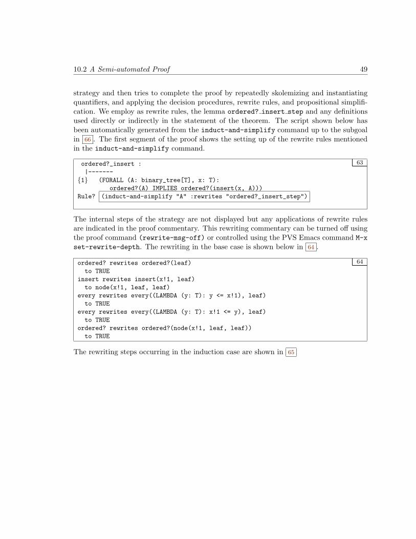
strategy and then tries to complete the proof by repeatedly skolemizing and instantiatingquantifiers, and applying the decision procedures, rewrite rules, and propositional simplifi-cation. We employ as rewrite rules, the lemma ordered? insert step and any definitionsused directly or indirectly in the statement of the theorem. The script shown below hasbeen automatically generated from the induct-and-simplify command up to the subgoalin 66 . The first segment of the proof shows the setting up of the rewrite rules mentionedin the induct-and-simplify command.

63ordered?_insert :|-------

1 (FORALL (A: binary_tree[T], x: T):ordered?(A) IMPLIES ordered?(insert(x, A)))

Rule? (induct-and-simplify "A" :rewrites "ordered?_insert_step")

The internal steps of the strategy are not displayed but any applications of rewrite rulesare indicated in the proof commentary. This rewriting commentary can be turned off usingthe proof command (rewrite-msg-off) or controlled using the PVS Emacs command M-xset-rewrite-depth. The rewriting in the base case is shown below in 64 .

64ordered? rewrites ordered?(leaf)to TRUE

insert rewrites insert(x!1, leaf)to node(x!1, leaf, leaf)

every rewrites every((LAMBDA (y: T): y <= x!1), leaf)to TRUE

every rewrites every((LAMBDA (y: T): x!1 <= y), leaf)to TRUE

ordered? rewrites ordered?(node(x!1, leaf, leaf))to TRUE

The rewriting steps occurring in the induction case are shown in 65


65ordered? rewrites ordered?(node(node1_var!1, node2_var!1, node3_var!1))to (every((LAMBDA (y: T): y <= node1_var!1), node2_var!1)


insert rewrites insert(x!1, node(node1_var!1, node2_var!1, node3_var!1))to (IF x!1 <= node1_var!1

THEN node(node1_var!1, insert(x!1, node2_var!1), node3_var!1)ELSE node(node1_var!1, node2_var!1, insert(x!1, node3_var!1))ENDIF)

ordered? rewritesordered?(node(node1_var!1, insert(x!1, node2_var!1), node3_var!1))to (every((LAMBDA (y: T): y <= node1_var!1), insert(x!1, node2_var!1))

AND every((LAMBDA (y: T): node1_var!1 <= y), node3_var!1)AND ordered?(insert(x!1, node2_var!1)) AND ordered?(node3_var!1))

ordered? rewritesordered?(node(node1_var!1, node2_var!1, insert(x!1, node3_var!1)))to (every((LAMBDA (y: T): y <= node1_var!1), node2_var!1)

ANDevery((LAMBDA (y: T): node1_var!1 <= y), insert(x!1, node3_var!1))

AND ordered?(node2_var!1) AND ordered?(insert(x!1, node3_var!1)))ordered?_insert_step rewritesevery((LAMBDA (y: T): y <= node1_var!1), insert(x!1, node2_var!1))to TRUE

One subgoal results from the induct-and-simplify command as shown in 66 . This sub-goal is nearly the same as subgoal ordered? insert.2.2 in 55 from the previous proofattempt. This means that the induct-and-simplify strategy completed the base case andmost of the induction branch of the proof automatically. The subgoal in 66 corresponds tothe case of insertion into the right subtree. The strategy failed to complete this branch of theproof because it was unable to apply the rewrite rule ordered? insert step automatically.This application failed because one of the conditions of the rewrite rule, node1 var!1 <=x!1, could not be discharged. This condition follows from formula number 1 in 66 and thelinearity of the <= relation. The latter constraint is, however, buried in the type constraint(total order?) of <=. This information has to be made explicit before the proof can besuccessfully completed.


66By induction on A, and by repeatedly rewriting and simplifying,this simplifies to:ordered?_insert :-1 ordered?(insert(node1_var!1, node2_var!1))-2 ordered?(insert(x!1, node3_var!1))-3 every((LAMBDA (y: T): y <= node1_var!1), node2_var!1)-4 every((LAMBDA (y: T): node1_var!1 <= y), node3_var!1)-5 ordered?(node2_var!1)-6 ordered?(node3_var!1)|-------

1 x!1 <= node1_var!12 every((LAMBDA (y: T): node1_var!1 <= y), insert(x!1, node3_var!1))

The rest of proof can be completed interactively as in the previous proof attempt butwe attempt a slightly different sequence of steps this time. The first step is identical to thatin 56 where the ordered? insert step lemma is manually invoked as a rewrite rule usingthe rewrite strategy.

67Rule? (rewrite "ordered?_insert_step")Found matching substitution:A gets node3_var!1,x gets x!1,pp gets (LAMBDA (y: T): node1_var!1 <= y),Rewriting using ordered?_insert_step,this simplifies to:ordered?_insert :[-1] ordered?(insert(node1_var!1, node2_var!1))[-2] ordered?(insert(x!1, node3_var!1))[-3] every((LAMBDA (y: T): y <= node1_var!1), node2_var!1)[-4] every((LAMBDA (y: T): node1_var!1 <= y), node3_var!1)[-5] ordered?(node2_var!1)[-6] ordered?(node3_var!1)|-------

1 node1_var!1 <= x!1[2] x!1 <= node1_var!1[3] every((LAMBDA (y: T): node1_var!1 <= y), insert(x!1, node3_var!1))

The next step is also identical to that of 58 where the type constraints for the <= operatorare explicitly introduced into the sequent.


68Rule? (typepred "obt.<=")Adding type constraints for obt.<=,this simplifies to:ordered?_insert :-1 total_order?[T](obt.<=)[-2] ordered?(insert(node1_var!1, node2_var!1))[-3] ordered?(insert(x!1, node3_var!1))[-4] every((LAMBDA (y: T): y <= node1_var!1), node2_var!1)[-5] every((LAMBDA (y: T): node1_var!1 <= y), node3_var!1)[-6] ordered?(node2_var!1)[-7] ordered?(node3_var!1)|-------

[1] node1_var!1 <= x!1[2] x!1 <= node1_var!1[3] every((LAMBDA (y: T): node1_var!1 <= y), insert(x!1, node3_var!1))

The main difference from the previous proof attempt is that we now invoke a somewhatpowerful variant of the all-purpose grind strategy where the :if-match flag is set to allindicating that all matching instances of any quantified formulas are to be used. If wedo not supply this option, the heuristic instantiator picks the wrong instance since thetype constraints for <= themselves provide matching instances for the one relevant typeconstraint, namely, dichotomous?(obt.<=).


69Rule? (grind :if-match all)

reflexive? rewrites reflexive?(obt.<=)to FORALL (x: T): obt.<=(x, x)

transitive? rewrites transitive?(obt.<=)to FORALL (x: T), (y: T), (z: T): obt.<=(x, y) & obt.<=(y, z) => obt.<=(x, z)

preorder? rewrites preorder?(obt.<=)to FORALL (x: T): obt.<=(x, x)

& FORALL (x: T), (y: T), (z: T):obt.<=(x, y) & obt.<=(y, z) => obt.<=(x, z)

antisymmetric? rewrites antisymmetric?(obt.<=)to FORALL (x: T), (y: T): obt.<=(x, y) & obt.<=(y, x) => x = y

partial_order? rewrites partial_order?(obt.<=)to (FORALL (x: T): obt.<=(x, x)

& FORALL (x: T), (y: T), (z: T):obt.<=(x, y) & obt.<=(y, z) => obt.<=(x, z))& FORALL (x: T), (y: T): obt.<=(x, y) & obt.<=(y, x) => x = y

dichotomous? rewrites dichotomous?(obt.<=)to (FORALL (x: T), (y: T): (obt.<=(x, y) OR obt.<=(y, x)))

total_order? rewrites total_order?[T](obt.<=)to ((FORALL (x: T): obt.<=(x, x)

& FORALL (x: T), (y: T), (z: T):obt.<=(x, y) & obt.<=(y, z) => obt.<=(x, z))

& FORALL (x: T), (y: T): obt.<=(x, y) & obt.<=(y, x) => x = y)& (FORALL (x: T), (y: T): (obt.<=(x, y) OR obt.<=(y, x)))

Trying repeated skolemization, instantiation, and if-lifting,Q.E.D.Run time = 48.86 secs.Real time = 230.49 secs.

The above semi-automated proof attempt illustrates the power that is gained fromcombining high-level strategies (e.g., induct-and-simplify and grind) to handle the easyportions of a proof with low-level manual interaction to carry out the more delicate steps.Note that the inner workings of these strategies which are hidden in the above proof canbe observed by invoking them with a $ suffix as in induct-and-simplify$ and grind$.

The proofs of the lemmas ordered? insert step in 27 and search insert shownin 70 below can be completed automatically by the single command:

(induct-and-simplify "A")


70search(x, A): RECURSIVE bool =(CASES A OFleaf: FALSE,node(y, B, C): (IF x = y THEN TRUE

ELSIF x<=y THEN search(x, B)ELSE search(x, C)

ENDIF)ENDCASES)

MEASURE size(A)

search_insert: THEOREM search(y, insert(x, A)) = (x = y OR search(y, A))

10.3 Proof Status

To conclude the development of binary trees and ordered binary trees, we can apply thePVS Emacs command M-x prt to recheck all the proofs and print out the proof status.3

The output of this command is shown below. It indicates that not only have all the theoremsbeen proved but so have any non-axioms (lemmas, TCCs, etc.) used in any of these proofs.

71Proof summary for theory obtordered?_TCC1..........................................proved - completeordered?_TCC2..........................................proved - completeinsert_TCC1............................................proved - completeinsert_TCC2............................................proved - completeordered?_insert_step...................................proved - completeordered?_insert........................................proved - completesearch_insert..........................................proved - completeTheory totals: 7 formulas, 7 attempted, 7 succeeded.

3The command M-x status-proof-theory or M-x spt can be used to get the proof status withoutrechecking the proofs.

Chapter 11

Built-in Datatype Simplifications

As indicated at the outset, the primary advantage of using abstract datatypes in PVS isthat a lot of knowledge about such datatypes and their operations is built into the system.To illustrate the sort of datatype simplifications that are built into PVS, consider the theorybinary props shown below.

55

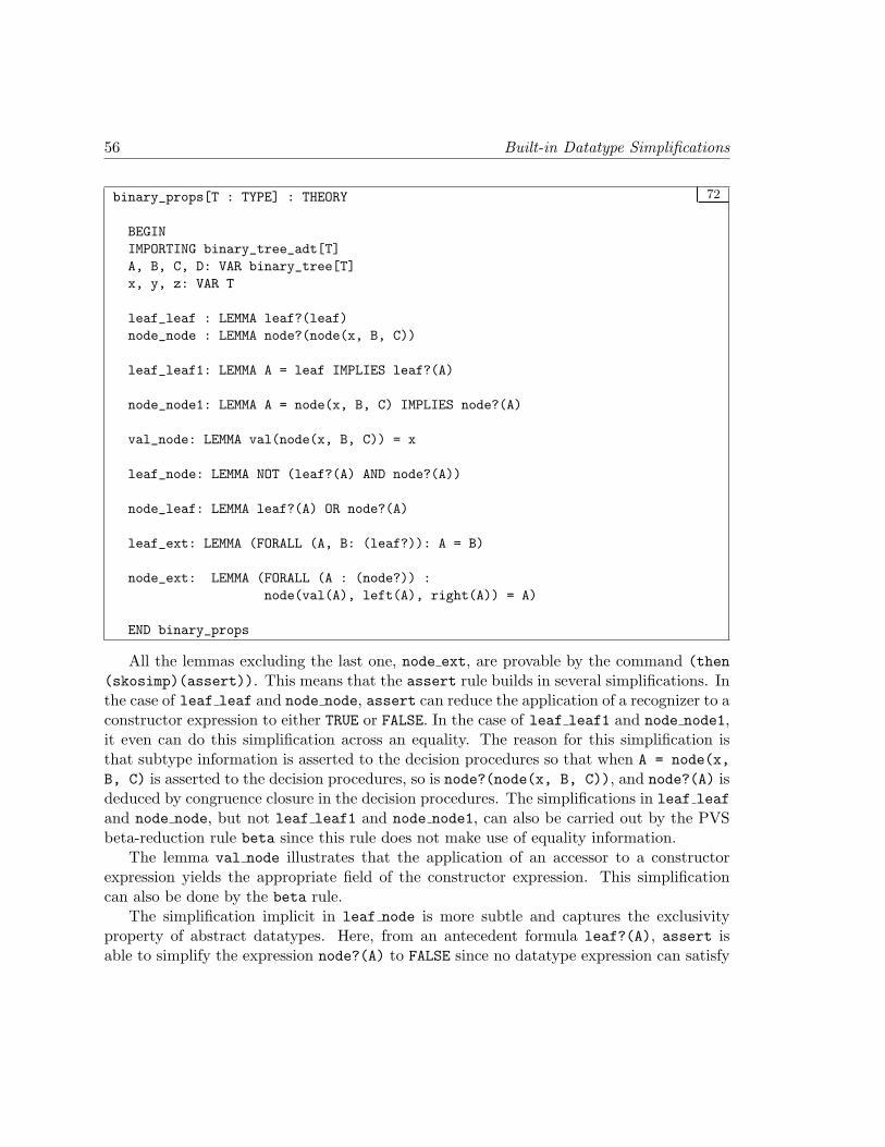
56 Built-in Datatype Simplifications

72binary_props[T : TYPE] : THEORY

BEGINIMPORTING binary_tree_adt[T]A, B, C, D: VAR binary_tree[T]x, y, z: VAR T

leaf_leaf : LEMMA leaf?(leaf)node_node : LEMMA node?(node(x, B, C))

leaf_leaf1: LEMMA A = leaf IMPLIES leaf?(A)

node_node1: LEMMA A = node(x, B, C) IMPLIES node?(A)

val_node: LEMMA val(node(x, B, C)) = x

leaf_node: LEMMA NOT (leaf?(A) AND node?(A))

node_leaf: LEMMA leaf?(A) OR node?(A)

leaf_ext: LEMMA (FORALL (A, B: (leaf?)): A = B)

node_ext: LEMMA (FORALL (A : (node?)) :node(val(A), left(A), right(A)) = A)

END binary_props

All the lemmas excluding the last one, node ext, are provable by the command (then(skosimp)(assert)). This means that the assert rule builds in several simplifications. Inthe case of leaf leaf and node node, assert can reduce the application of a recognizer to aconstructor expression to either TRUE or FALSE. In the case of leaf leaf1 and node node1,it even can do this simplification across an equality. The reason for this simplification isthat subtype information is asserted to the decision procedures so that when A = node(x,B, C) is asserted to the decision procedures, so is node?(node(x, B, C)), and node?(A) isdeduced by congruence closure in the decision procedures. The simplifications in leaf leafand node node, but not leaf leaf1 and node node1, can also be carried out by the PVSbeta-reduction rule beta since this rule does not make use of equality information.

The lemma val node illustrates that the application of an accessor to a constructorexpression yields the appropriate field of the constructor expression. This simplificationcan also be done by the beta rule.

The simplification implicit in leaf node is more subtle and captures the exclusivityproperty of abstract datatypes. Here, from an antecedent formula leaf?(A), assert isable to simplify the expression node?(A) to FALSE since no datatype expression can satisfy

Built-in Datatype Simplifications 57

two recognizers. The simplification implicit in node leaf captures the inclusivity propertyof abstract datatypes. Here, assert is able to determine that a recognizer holds of anexpression by demonstrating that all the other recognizers are false on the expression. Ingeneral, when confronted with the application of a recognizer r to a datatype expression e,the simplifier evaluates the truth value of each recognizer of that datatype when applied tothe given expression using the decision procedures. If r(e) is determined to be TRUE by thedecision procedures, then r(e) is obviously simplified to TRUE by the simplifier. If for someother recognizer r′, r′(e) is determined to be TRUE by the decision procedures, then r(e) issimplified to FALSE. If for all recognizers r′ distinct from r, r′(e) is determined to be FALSE,then r(e) is simplified to TRUE.

The lemma leaf ext essentially illustrates that for constructors such as leaf that haveno accessors, there is no distinction between the forms leaf?(A) and A = leaf. It alsoillustrates how the subtype information is used implicitly to simplify A = B to TRUE.

The lemma node ext is the only one that cannot be proved by the command (then(skosimp)(assert)). Here, this command simplifies the goal sequent to a single sub-goal that is then proved by means of the (apply-extensionality) command. This il-lustrates that the extensionality axiom for datatypes is built into the primitive PVS ruleextensionality and is also employed by the strategies replace-extensionality andapply-extensionality.

58 Built-in Datatype Simplifications

Chapter 12

Some Proof Strategies

We briefly explain the definitions of the proof strategies induct-and-simplify andgrind that were used in Section 10. The PVS manuals [OSRSC98] provides more de-tails. These strategies are quite useful for proofs of datatype-related theorems. Theinduct-and-simplify strategy takes an argument list of the form:

(var &optional (fnum 1) name (defs t) (if-match best)theories rewrites exclude)

where

• var is the induction variable and is the only required argument

• fnum is the formula number of the induction formula where the induction variable isuniversally quantified; it defaults to 1

• name names the induction scheme to be employed

• defs indicates which definitions of constants used in the current goal are to be installedas rewrite rules; it defaults to t indicating that all relevant definitions must be installed

• if-match instructs the heuristic instantiator to use none, one, all, or the best matchinginstantiation for a quantified formula; it defaults to best

• theories is the list of theories to be installed as rewrite rules

• rewrites is the list of formulas or definitions that are to be installed as rewrite rules,and

• exclude is a list of formulas or definitions that should be removed from the rewriterule base

59

60 Some Proof Strategies

The body of the definition of the strategy has the form:

(then(install-rewrites$ :defs defs :theories theories :rewrites rewrites:exclude exclude)(try (induct var fnum name)(then (skosimp*) (assert) (repeat (lift-if))(repeat*(then (assert) (bddsimp) (skosimp*)(if if-match (inst? :if-match if-match) (skip)) (lift-if))))

(skip)))

The induct-and-simplify strategy first installs the rewrites using install-rewrites$on defs, theories, rewrites, and exclude. It then introduces the appropriate instanceof the induction scheme using induct. Then the strategy carries out one round of skolem-ization (introduction of new constants for outermost universally bound variables) usingskosimp*, rewriting and simplification using assert, and repeated lifting of condition-als to the top level using lift-if. Following this, there are repeated rounds of rewrit-ing/simplification, propositional simplification, skolemization, heuristic instantiation, andif-lifting until each resulting subgoal has stabilized.

The grind strategy is similar. It takes the following argument list:

(&optional (defs !) theories rewrites exclude (if-match t) (updates? t))

where the only new argument from induct-and-simplify is updates? which when set toNIL blocks the if-lifting of update applications of the form (A WITH [(i) := b])(j) to(IF i = j THEN b ELSE A(j) ENDIF).

The body of the definition of grind is:

(then(install-rewrites$ :defs defs :theories theories :rewrites rewrites:exclude exclude)(then (bddsimp) (assert)) (replace*)(reduce$ :if-match if-match :updates? updates?))

Here the rewrite rules are installed using install-rewrites$, and followed by propo-sitional simplification, rewriting and simplification, equality replacement, followed by re-peated applications of these steps along with heuristic instantiation and if-lifting.

It should be clear from the above definition that it is fairly straightforward to writepowerful proof strategies using the constructs provided by the PVS proof checker.

Chapter 13

Limitations of the PVS AbstractDatatype Mechanism

The abstract datatype mechanism of PVS is intended to capture a fairly large class ofdatatypes whose axioms can be easily and systematically generated. This class contains allthe freely generated term algebras over an order-sorted signature which includes the variousstack and tree-like data structures. It excludes such important datatypes as integers (whichare built into PVS), bags, sets, and queues. It also excludes various lazy data structuressuch as lazy lists or streams. These latter structures can be introduced by implementing asimilar mechanism for introducing co-datatypes as for datatypes.

The DATATYPE mechanism is a primitive construct of PVS and is not merely a defini-tional extension of PVS. It therefore has the disadvantage that it is not possible to provegeneral theorems about all recursive datatypes in the way that one can about all inductivedefinitions given as least fixed points. For example, Bird’s fusion theorem [Bir95] cannotbe uniformly proved for all recursive datatypes and has to be proved for each datatypeindividually [Sha96].

61

62 Limitations of the PVS Abstract Datatype Mechanism

Chapter 14

Related Work

There are a number of algebraic specification languages such as Larch [GJMW93],OBJ [FGJM85], and ACT-ONE [EM85] that can be used to specify abstract datatypesbut these specifications are manually axiomatized and not automatically generated from asuccinct description as is the case with the PVS DATATYPE construct. The axioms are usedas rewrite rules so that there is no built-in automation of the simplification of datatypeexpressions.

The programming language ML [MTH90] has a similar recursive datatype mechanism.Unlike the PVS mechanism, the ML construct allows arbitrary forms of recursion. As notedearlier, such recursive type definitions do not always have a proper set-theoretic semantics.Gunter [Gun93] explains how certain recursive datatypes that are admissible in ML canlead to unsoundnesses if admitted into a higher-order logic.

The HOL system has a mechanism for defining abstract datatypes [Mel89] that is some-what more restrictive than that of PVS: there are more constraints on recursion and HOLlacks the useful notion of subtyping that is available in PVS. However, the HOL constructis definitional in that a recursively specified datatype is defined in terms of the primitivetype constructors available in HOL. In particular, any newly defined recursive datatype isshown to be interpretable as a subset of some existing datatype based on finitely branchingtrees. The axioms generated from the datatype declaration are shown to be sound withrespect to this interpretation. Isabelle/ZF and Isabelle/HOL both have a similar but moregeneral facility for defining datatypes and co-datatypes [Pau97]. The Isabelle datatypemechanism also accomodates infinitely branching trees. The Coq system has a facility fordefining recursive and co-recursive datatypes which, like PVS and unlike HOL and Isabelle,is a primitive construct of the Coq logic [Gim96].

The shell principle used in the Boyer-Moore theorem prover [BM79, BM88] is quitesimilar to the PVS DATATYPE mechanism. It permits recursive datatypes to be specified bymeans of constructors, accessors, and recognizers. Like PVS, the axioms corresponding to

63

64 Related Work

a shell datatype are built into the inference mechanisms of the theorem prover. The shellprinciple, however, has many serious limitations. It is complicated by the lack of types orsubtypes in the Boyer-Moore logic. The shell principle only allows one constructor and abottom object thus ruling out a great many useful datatypes where multiple constructorsare required.

Chapter 15

Conclusions

We have described the DATATYPE mechanism of PVS and demonstrated its use in proofconstruction. This mechanism captures a large class of commonly used type definitionswithin a succinct notation. A number of facts about these automatically generated abstractdatatypes are built into the inference mechanisms of PVS so that it is possible to obtaina significant degree of automation when proving theorems involving datatypes. The highlevel of automation in the low-level inference mechanisms in PVS makes it easy to definepowerful and flexible high-level proof strategies.

15.0.0.13 Acknowledgements.

The design and implementation of PVS was directed by John Rushby of the SRI ComputerScience Laboratory. He, along with Rick Butler of NASA and Mandayam Srivas, suggestedseveral improvements to this document. Donald Syme of Cambridge University carefullyproofread the document and gave numerous helpful suggestions. We are also grateful toUlrich Hensel of TU Dresden for his as yet unheeded suggestion to incorporate corecursivedatatypes.

65

66 Conclusions

Bibliography

[Bir95] Richard S. Bird. Functional algorithm design. In Bernhard Moller, editor,Mathematics of Program Construction ’95, number 947 in Lecture Notes inComputer Science, pages 2–17. Springer-Verlag, 1995. 61

[BM79] R. S. Boyer and J S. Moore. A Computational Logic. Academic Press, NewYork, NY, 1979. 1, 63

[BM88] R. S. Boyer and J S. Moore. A Computational Logic Handbook. AcademicPress, New York, NY, 1988. 63

[EM85] H. Ehrig and B. Mahr. Fundamentals of Algebraic Specification 1. Springer-Verlag, Berlin, 1985. 63

[FGJM85] Kokichi Futatsugi, Joseph Goguen, Jean-Pierre Jouannaud, and Jose Meseguer.Principles of OBJ2. In Brian K. Reid, editor, 12th ACM Symposium on Princi-ples of Programming Languages, pages 52–66. Association for Computing Ma-chinery, 1985. 63

[Gim96] Eduardo Gimenez. A tutorial on recursive types in Coq. Draft. Availablefrom ftp://cri.ens-lyon.fr/pub/LIP/COQ/V6.1.beta/doc/RecTutorial.ps.gz, March 1996. 63

[GJMW93] John V. Guttag and James J. Horning with S. J. Garland, K. D. Jones,A. Modet, and J. M. Wing. Larch: Languages and Tools for Formal Speci-fication. Texts and Monographs in Computer Science. Springer-Verlag, 1993.63

[GMW79] M. Gordon, R. Milner, and C. Wadsworth. Edinburgh LCF: A Mechanized Logicof Computation, volume 78 of Lecture Notes in Computer Science. Springer-Verlag, 1979. 35

[Gun93] Elsa L. Gunter. Why we can’t have SML style datatype declarations in HOL.In L. J. M. Claesen and M. J. C. Gordon, editors, Higher Order Logic Theorem

67

ftp://cri.ens-lyon.fr/pub/LIP/COQ/V6.1.beta/doc/RecTutorial.ps.gz

ftp://cri.ens-lyon.fr/pub/LIP/COQ/V6.1.beta/doc/RecTutorial.ps.gz

68 BIBLIOGRAPHY

Proving and its Applications, number 20 in IFIP Transactions A, pages 561–568. North-Holland, 1993. 63

[HJ97] Ulrich Hensel and Bart Jacobs. Proof principles for datatypes with iteratedrecursion. In Category Theory in Computer Science, 1997. Also appears asTechnical Report CSI-R9703, Computing Science Institute, Faculty of Mathe-matics and Informatics, Catholic University of Nijmegen. 2

[Mel89] Thomas F. Melham. Automating recursive type definitions in higher orderlogic. In G. Birtwistle and P. A. Subrahmanyam, editors, Current Trends inHardware Verification and Theorem Proving, pages 341–386, New York, NY,1989. Springer-Verlag. 63

[MTH90] R. Milner, M. Tofte, and R. Harper. The Definition of Standard ML. MITPress, 1990. 63

[OSRSC98] S. Owre, N. Shankar, J. M. Rushby, and D. W. J. Stringer-Calvert. User Guidefor the PVS Specification and Verification System. Computer Science Labo-ratory, SRI International, Menlo Park, CA, September 1998. Three volumes:Language, System, and Prover Reference Manuals. 1, 59

[Pau97] L. C. Paulson. Mechanizing coinduction and corecursion in higher-order logic.Journal of Logic and Computation, 7:175–204, March 1997. 63

[Pet67] R. Peter. Recursive Functions. Academic Press, New York, NY, 1967. 31

[Rus95] John Rushby. Proof Movie II: A proof with PVS. Technical report, ComputerScience Laboratory, SRI International, Menlo Park, CA, 1995. Available, withspecification files, at http://www.csl.sri.com/movie.html. 25

[Sha96] N. Shankar. Steps towards mechanizing program transformations using PVS.Science of Computer Programming, 26(1–3):33–57, 1996. 61

[WW93] Debora Weber-Wulff. Proof Movie—a proof with the Boyer-Moore prover.Formal Aspects of Computing, 5(2):121–151, 1993. 25

http://www.csl.sri.com/movie.html

abstract datatypes in pvs - pvs specification...

Documents