DEFORMABLE MODELS WITH APPLICATION TO HUMAN

CEREBRAL CORTEX RECONSTRUCTION FROM MAGNETIC

RESONANCE IMAGES

by

Chenyang Xu

A dissertation submitted to the Johns Hopkins University in conformity with the

requirements for the degree of Doctor of Philosophy

Baltimore, Maryland

January, 1999

c Chenyang Xu 1999

All rights reserved

Abstract

Constructing a mathematical representation of an object boundary (boundary map-

ping) from images is an important problem that is of importance to several active

research areas such as image analysis, computer vision, and medical imaging. The

focus of this dissertation is to investigate deformable models, a boundary mapping

technique that incorporates both image information and prior knowledge about the

boundary geometry to extract a meaningful boundary description. A key problem

with methods reported in the literature is that they have diÆculties in reliably map-

ping boundaries when the models are not initialized near target boundaries or are

applied to reconstruct boundaries with concavities.

In this research, we make three main contributions to the area of boundary map-

ping. First, we developed a method called the gradient vector ow deformable model

that is robust to both model initialization and boundary concavities. Second, we

developed a generalization of the �rst method that allows for improved performance

in converging to narrow boundary indentations and greater accuracy in localizing

boundaries. Third, we developed a method for reconstructing the central layer of the

human cerebral cortex from magnetic resonance images that uses our proposed de-

formable model as a core component. Our methods are validated on both simulated

images and real magnetic resonance images.

This thesis is prepared under the direction of Dr. Jerry L. Prince.

ii

Acknowledgements

I would like to thank my research advisor, Dr. Jerry L. Prince, for his friendship,

encouragement, and guidance during the course of my research. He has been a valu-

able source of ideas and stimulating discussions on both technical and non-technical

topics. It has been my great fortune and honor to earn my degree under his super-

vision. I would like to thank those who served as members of my Graduate Board

Oral committee. Their time and energy is gratefully acknowledged. I would like to

thank Dr. John Goutsias, Dr. Howard L. Weinert, and Dr. Lawrence B. Wol� for

their supportive role throughout my graduate student career. I would like to thank

both Dr. Michael I. Miller and Dr. Howard L. Weinert for their helpful comments

and suggestions in helping this dissertation take its �nal form. Both the assistance

of the faculty and sta� and the �nancial support from the Department of Electrical

and Computer Engineering throughout the years deserves much appreciation. The

support of the National Science Foundation is gratefully acknowledged.

I would like to thank all of my colleagues and friends whose friendship and en-

couragement have made my experience at the Johns Hopkins University a memorable

one. In particular, I would like to thank Dzung L. Pham for his helpful input and

stimulating discussions regarding my research as well as his proofreading of my tech-

nical publications to improve their overall presentation quality. I would like to thank

Maryam E. Etemad and Daphne N. Yu for their assistance in processing brain MR

data for my research and proofreading several papers. I would like to thank Diego So-

colinsky for pointing out the references to the solvability of the GVF Euler equation.

I would like to thank Carol Prince who has prepared desserts for our weekly group

meeting throughout the years, which is no doubt a great source of energy and sup-

port to my research. I would like to thank Dr. Nick Bryan, Dr. Christos Davatzikos,

and Dr. Susan Resnick for having many helpful discussions on brain mapping and

providing much needed data and expertise. I would like to thank Dr. Ron Kikinis at

the Harvard Medical School for providing brain MR data used in this research.

Finally I would like to thank my parents Dechang Xu and Yongtuan Yang and

my brother Chenguan Xu back home for all that they have done for me. I would

especially like to thank my wife Wei Shu who with her patience, understanding, and

love has helped me to achieve this goal. This dissertation is dedicated to them.

iii

Contents

Abstract ii

Acknowledgements iii

List of Figures vii

List of Tables xi

1 Introduction 1

1.1 Deformable Models . . . . . . . . . . . . . . . . . . . . . . . . . . . . 3

1.2 Related Work . . . . . . . . . . . . . . . . . . . . . . . . . . . . . . . 41.3 Brain Cortex Reconstruction . . . . . . . . . . . . . . . . . . . . . . . 61.4 Thesis Contributions . . . . . . . . . . . . . . . . . . . . . . . . . . . 8

1.5 Previous Publications . . . . . . . . . . . . . . . . . . . . . . . . . . . 9

1.6 Thesis Organization . . . . . . . . . . . . . . . . . . . . . . . . . . . . 9

2 Background 10

2.1 Deformable Contours . . . . . . . . . . . . . . . . . . . . . . . . . . . 10

2.2 Deformable Surfaces . . . . . . . . . . . . . . . . . . . . . . . . . . . 12

3 Gradient Vector Flow Deformable Models 14

3.1 Behavior of Traditional Deformable Contours . . . . . . . . . . . . . 15

3.2 Generalized Force Balance Equations . . . . . . . . . . . . . . . . . . 19

3.3 Gradient Vector Flow Deformable Contour . . . . . . . . . . . . . . . 20

3.3.1 Edge Map . . . . . . . . . . . . . . . . . . . . . . . . . . . . . 21

3.3.2 Gradient Vector Flow . . . . . . . . . . . . . . . . . . . . . . . 22

3.3.3 Numerical Implementation . . . . . . . . . . . . . . . . . . . . 233.4 GVF Fields and Deformable Contours: Demonstrations . . . . . . . . 25

3.4.1 Convergence to Boundary Concavity . . . . . . . . . . . . . . 25

3.4.2 Streamlines . . . . . . . . . . . . . . . . . . . . . . . . . . . . 27

3.4.3 Deformable Contour Initialization and Convergence . . . . . . 29

3.5 Gray-level Images and Higher Dimensions . . . . . . . . . . . . . . . 32

iv

3.5.1 Gray-level Images . . . . . . . . . . . . . . . . . . . . . . . . . 32

3.5.2 Higher Dimensions . . . . . . . . . . . . . . . . . . . . . . . . 33

3.6 Summary . . . . . . . . . . . . . . . . . . . . . . . . . . . . . . . . . 38

3.A Derivation of the GVF Euler Equation . . . . . . . . . . . . . . . . . 383.B Metaspheres . . . . . . . . . . . . . . . . . . . . . . . . . . . . . . . . 40

4 Generalized Gradient Vector Flow Deformable Models 43

4.1 Generalized GVF . . . . . . . . . . . . . . . . . . . . . . . . . . . . . 44

4.2 Experimental Results . . . . . . . . . . . . . . . . . . . . . . . . . . . 46

4.3 GGVF and Shape Analysis . . . . . . . . . . . . . . . . . . . . . . . . 53

4.4 GGVF and the Central Layer of Thick Boundaries . . . . . . . . . . . 584.5 Variational Framework for Generalizing GVF . . . . . . . . . . . . . . 60

4.6 Summary . . . . . . . . . . . . . . . . . . . . . . . . . . . . . . . . . 63

5 Human Cerebral Cortex Reconstruction from MR Images 64

5.1 Methods . . . . . . . . . . . . . . . . . . . . . . . . . . . . . . . . . . 655.1.1 Data Acquisition and Preprocessing . . . . . . . . . . . . . . . 65

5.1.2 Fuzzy Segmentation of GM, WM and CSF . . . . . . . . . . . 665.1.3 Estimation of Initial Surface with the Correct Topology . . . . 695.1.4 Re�nement of the Initial Surface Using a Deformable Surface

Model . . . . . . . . . . . . . . . . . . . . . . . . . . . . . . . 76

5.1.5 Reconstructed Surface . . . . . . . . . . . . . . . . . . . . . . 79

5.2 Results . . . . . . . . . . . . . . . . . . . . . . . . . . . . . . . . . . . 815.2.1 Qualitative Results . . . . . . . . . . . . . . . . . . . . . . . . 82

5.2.2 Quantitative Results . . . . . . . . . . . . . . . . . . . . . . . 82

5.3 Applications . . . . . . . . . . . . . . . . . . . . . . . . . . . . . . . . 915.3.1 Cortical Di�erential Geometry and Thickness Computation . . 915.3.2 A Spherical Map for Cortical Geometry . . . . . . . . . . . . . 93

5.4 Summary . . . . . . . . . . . . . . . . . . . . . . . . . . . . . . . . . 945.A Landmark Picking and Landmark Errors . . . . . . . . . . . . . . . . 95

6 Conclusions and Future Work 97

6.1 Gradient Vector Flow Deformable Models . . . . . . . . . . . . . . . 97

6.1.1 Main Results . . . . . . . . . . . . . . . . . . . . . . . . . . . 986.1.2 Future Work . . . . . . . . . . . . . . . . . . . . . . . . . . . . 98

6.2 Generalized Gradient Vector Flow Deformable Models . . . . . . . . . 99

6.2.1 Main Results . . . . . . . . . . . . . . . . . . . . . . . . . . . 99

6.2.2 Future Work . . . . . . . . . . . . . . . . . . . . . . . . . . . . 100

6.3 Brain Cortex Reconstruction . . . . . . . . . . . . . . . . . . . . . . . 100

6.3.1 Main Results . . . . . . . . . . . . . . . . . . . . . . . . . . . 101

6.3.2 Future Work . . . . . . . . . . . . . . . . . . . . . . . . . . . . 101

6.4 Overall Perspective . . . . . . . . . . . . . . . . . . . . . . . . . . . . 102

v

A Deformable Model Implementation 103

A.1 Deformable Contours . . . . . . . . . . . . . . . . . . . . . . . . . . . 103

A.2 Deformable Surfaces . . . . . . . . . . . . . . . . . . . . . . . . . . . 104

A.2.1 Simplex Meshes: a Surface Representation for Deformable Sur-faces . . . . . . . . . . . . . . . . . . . . . . . . . . . . . . . . 105

A.2.2 Triangle Mesh Generation . . . . . . . . . . . . . . . . . . . . 107

A.2.3 Simplex Mesh Generation through Dual Operation on Triangle

Meshes . . . . . . . . . . . . . . . . . . . . . . . . . . . . . . . 110

A.2.4 Deformable Surface Implementation . . . . . . . . . . . . . . . 112

B Di�erential Geometry Quantities on Simplex Meshes 115

Bibliography 120

vi

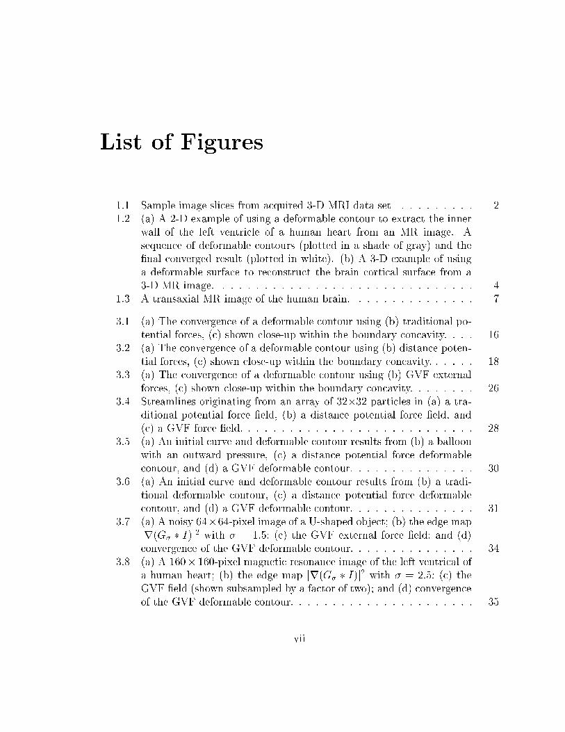
List of Figures

1.1 Sample image slices from acquired 3-D MRI data set . . . . . . . . . 2

1.2 (a) A 2-D example of using a deformable contour to extract the inner

wall of the left ventricle of a human heart from an MR image. A

sequence of deformable contours (plotted in a shade of gray) and the

�nal converged result (plotted in white). (b) A 3-D example of using

a deformable surface to reconstruct the brain cortical surface from a3-D MR image. . . . . . . . . . . . . . . . . . . . . . . . . . . . . . . 4

1.3 A transaxial MR image of the human brain. . . . . . . . . . . . . . . 7

3.1 (a) The convergence of a deformable contour using (b) traditional po-tential forces, (c) shown close-up within the boundary concavity. . . . 16

3.2 (a) The convergence of a deformable contour using (b) distance poten-

tial forces, (c) shown close-up within the boundary concavity. . . . . . 18

3.3 (a) The convergence of a deformable contour using (b) GVF external

forces, (c) shown close-up within the boundary concavity. . . . . . . . 263.4 Streamlines originating from an array of 32�32 particles in (a) a tra-

ditional potential force �eld, (b) a distance potential force �eld, and

(c) a GVF force �eld. . . . . . . . . . . . . . . . . . . . . . . . . . . . 283.5 (a) An initial curve and deformable contour results from (b) a balloon

with an outward pressure, (c) a distance potential force deformablecontour, and (d) a GVF deformable contour. . . . . . . . . . . . . . . 30

3.6 (a) An initial curve and deformable contour results from (b) a tradi-

tional deformable contour, (c) a distance potential force deformablecontour, and (d) a GVF deformable contour. . . . . . . . . . . . . . . 31

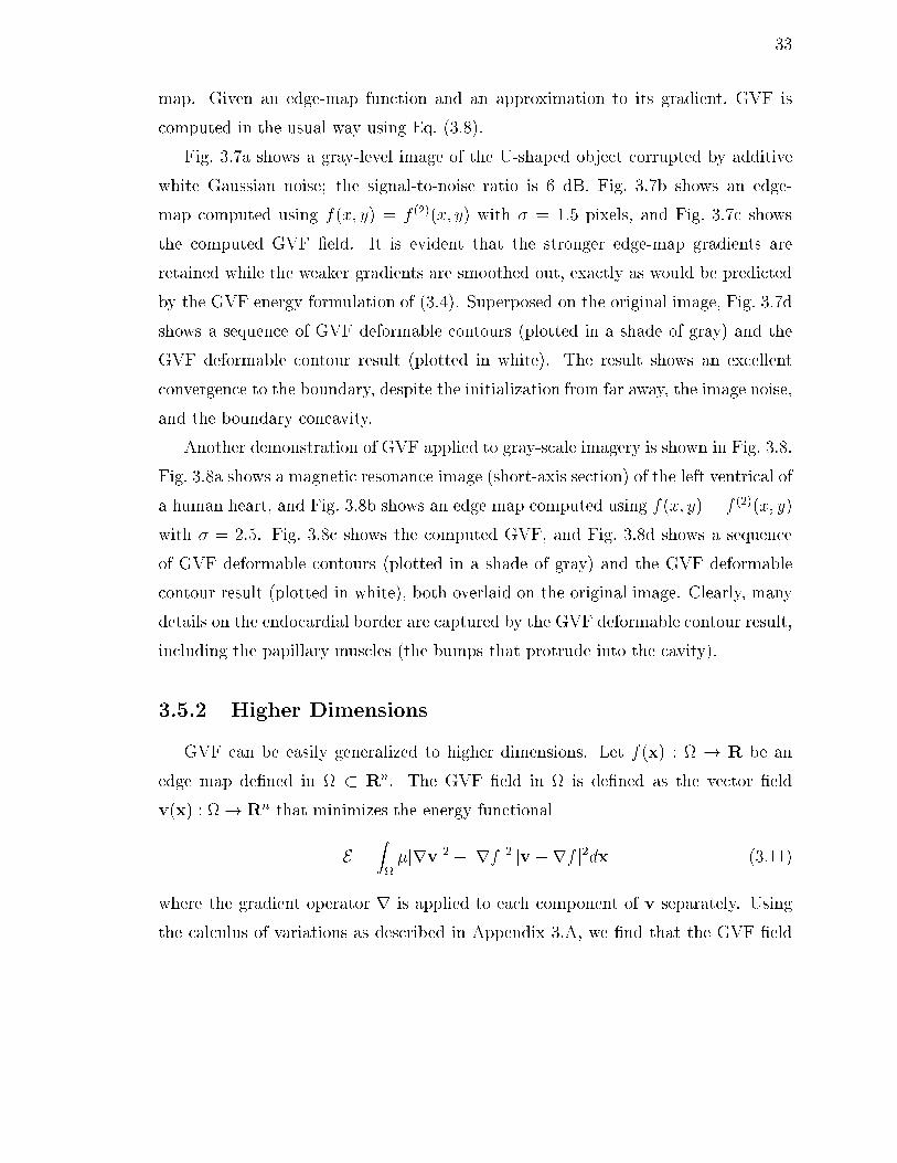
3.7 (a) A noisy 64�64-pixel image of a U-shaped object; (b) the edge map

jr(G� � I)j2 with � = 1:5; (c) the GVF external force �eld; and (d)convergence of the GVF deformable contour. . . . . . . . . . . . . . . 34

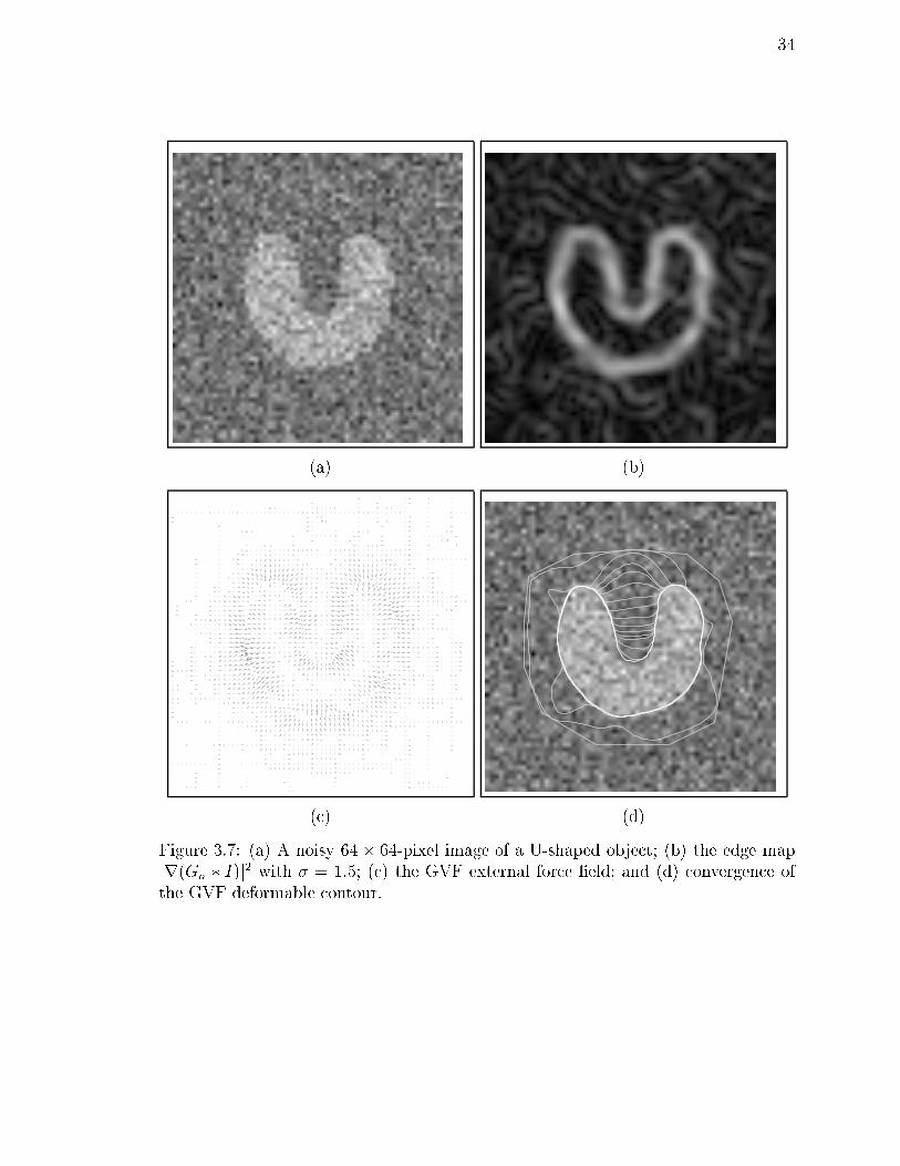
3.8 (a) A 160� 160-pixel magnetic resonance image of the left ventrical ofa human heart; (b) the edge map jr(G� � I)j2 with � = 2:5; (c) the

GVF �eld (shown subsampled by a factor of two); and (d) convergence

of the GVF deformable contour. . . . . . . . . . . . . . . . . . . . . . 35

vii

3.9 (a) Isosurface of a 3-D object de�ned on a 643 grid; (b) positions of

planes A and B on which the 3-D GVF vectors are depicted in (c) and

(d), respectively; (e) the initial con�guration of a deformable surface

using GVF and its positions after (f) 10, (g) 40, and (h) 100 iterations. 373.10 Sample metaspheres: (a) a = (2; 2; 2), b = 0, m = 0, n = 0, and

c = 0; (b) a = (2; 2; 1), b = (0:5; 0:5; 0), m = 0, n = (6; 6; 6), and

c = 0; (c) a = (2; 2; 2), b = (0:5; 0:5; 0), m = (4; 4; 4), n = (4; 4; 4),

and c = 0; and (d) a = (2; 0:5; 0:5), b = 0, m = 0, n = 0, and c = �0:4. 424.1 Plots of both (a) the GVF and (b) the GGVF weighting functions. . 46

4.2 (a) A square with a long, thin indentation and broken boundary; (b)

original GVF �eld (zoomed); (c) proposed GGVF �eld (zoomed); (d)

initial contour position for both the GVF deformable contour and theGGVF deformable contour; (e) �nal result of the GVF deformable

contour; and (f) �nal result of the GGVF deformable contour. . . . . 474.3 Harmonic curves: r = a + b cos(m� + c) . . . . . . . . . . . . . . . . . 49

4.4 Maximum radial error (MRE). . . . . . . . . . . . . . . . . . . . . . . 504.5 (a) Impulse noise corrupted image and the initial deformable contour;

(b) and (c) deformable contour results using traditional external forces

r(G�(x; y)� I(x; y)) where � = 1 and 9; (d) deformable contour resultusing distance potential force; (e) GVF deformable contour result with� = 0:1; and (f) GGVF deformable contour result with � = 0:2. The

edge map used for both GVF and GGVF is f = G�(x; y)�I(x; y), where� = 1, respectively. All deformable contour results are computed using

� = 0:25 and � = 0. . . . . . . . . . . . . . . . . . . . . . . . . . . . . 514.6 (a) A 160� 160-pixel magnetic resonance image of the left ventrical of

a human heart; (b) the edge map jr(G�(x; y) � I(x; y))j2 with � = 2:5;

(c) the result of GVF deformable contour with � = 0:1; and (d) theresult of GGVF deformable contour with � = 0:15. The parameters

used for both deformable contours are � = 0:1 and � = 0. . . . . . . . 544.7 GGVF �elds computed from objects with various shapes. . . . . . . . 56

4.8 The magnitude of the GVF �eld gives information about the medial

axis of a shape. . . . . . . . . . . . . . . . . . . . . . . . . . . . . . . 57

4.9 The medialness map M1(x; y) (q = 0:05) of a teardrop shape, shown

as (a) a gray-level image and (b) a surface plot. . . . . . . . . . . . . 58

4.10 GGVF vector �eld converges to the center of a thick edge. . . . . . . 594.11 GGVF deformable contour results from simulated images with bound-

ary thickness equal to 3 pixels (a)-(c), 6 pixels (d)-(f), and 9 pixels(g)-(i). . . . . . . . . . . . . . . . . . . . . . . . . . . . . . . . . . . . 61

4.12 Maximum radial error for thick boundaries (MRE). . . . . . . . . . . 62

5.1 Block diagram of the overall cortical surface reconstruction system. . 65

viii

5.2 Sample slices from acquired MRI data set. . . . . . . . . . . . . . . . 67

5.3 Sample slices after the cerebral tissue extraction. . . . . . . . . . . . . 68

5.4 Sample slice from membership functions computed using AFCM. (a)

GM, (b) WM, and (c) CSF. . . . . . . . . . . . . . . . . . . . . . . . 705.5 Resolution problems in determining the cortical surface. (a) ideal im-

age, and (b) sampled image. . . . . . . . . . . . . . . . . . . . . . . . 71

5.6 (a) Isosurface of WM membership function with the incorrect topology,

(b) estimated initial surface with the correct topology. . . . . . . . . . 75

5.7 Illustration of behavior of C(x). . . . . . . . . . . . . . . . . . . . . . 77

5.8 Initial deformable contour shown in black and �nal converged contour

shown in white. . . . . . . . . . . . . . . . . . . . . . . . . . . . . . . 78

5.9 A surface rendering of reconstructed cortical surface from one subject

displayed from multiple views: (a) top, (b) bottom, (c) left, (d) right,

(e) left medial, and (f) right medial. . . . . . . . . . . . . . . . . . . . 80

5.10 Cross sectional views of the reconstructed cortical surface: (a) axial,

(b) coronal, and (c) sagittal. . . . . . . . . . . . . . . . . . . . . . . . 815.11 Medial view of surface rendering of all six reconstructed cortical surface. 835.12 From left to right and top to bottom, the coronal slice across the ante-

rior commissure for subjects 1 to 6 superimposed with the cross sectionof the corresponding reconstructed cortical surface. . . . . . . . . . . 84

5.13 Surface renderings of (a) shrink-wrapping method versus (b) proposed

method. Cross-sections of (c) shrink-wrapping method versus (d) pro-posed method. . . . . . . . . . . . . . . . . . . . . . . . . . . . . . . . 89

5.14 (a) Front and (b) lateral views of a cortical mean curvature map. (c)Colormap used for plotting the map. . . . . . . . . . . . . . . . . . . 91

5.15 (a) Front and (b) lateral views of a cortical thickness map. (c) Col-

ormap used for plotting the map. . . . . . . . . . . . . . . . . . . . . 925.16 (a) A spherical map depicting mean curvature. The central sulcus is

outlined in black. (b) Manually identi�ed central sulcus. . . . . . . . 945.17 Manually identi�ed sulci on (a) the spherical map, and (b) the cortical

surface. . . . . . . . . . . . . . . . . . . . . . . . . . . . . . . . . . . 95

5.18 Illustration of the con�guration of ideal landmark, actual landmark,and closest point on the surface. . . . . . . . . . . . . . . . . . . . . . 96

A.1 (a) a loop; (b) double edges. . . . . . . . . . . . . . . . . . . . . . . . 106

A.2 A simplex mesh. . . . . . . . . . . . . . . . . . . . . . . . . . . . . . . 106

A.3 Illustration of a dual operation. . . . . . . . . . . . . . . . . . . . . . 107

A.4 A triangle and its subdivided triangles. . . . . . . . . . . . . . . . . . 108

A.5 Subdividing to improve a triangular approximation to a sphere. . . . 109

A.6 Surface rendering of a brain triangle mesh obtained by computing the

isosurface from a brain image volume and its zoom view with edges

superimposed on the mesh. . . . . . . . . . . . . . . . . . . . . . . . . 110

ix

A.7 The dual meshes of meshes shown in Fig. A.5. . . . . . . . . . . . . . 112

A.8 The dual mesh of the mesh shown in Fig. A.6. . . . . . . . . . . . . . 113

A.9 Vertex structure on a simplex mesh. . . . . . . . . . . . . . . . . . . . 114

B.1 Unit normal estimation using three neighboring nodes. . . . . . . . . 116

x

List of Tables

5.1 Size and Euler characteristics of meshes from the original isosurface

calculation. . . . . . . . . . . . . . . . . . . . . . . . . . . . . . . . . 74

5.2 Euler characteristic of largest resulting surface after each iteration. . . 74

5.3 Euler characteristics of surfaces generated for six subjects at di�erent

iterations. . . . . . . . . . . . . . . . . . . . . . . . . . . . . . . . . . 85

5.4 GM percentage measure of reconstructed surfaces for six subjects . . 855.5 Landmark errors (in mm) . . . . . . . . . . . . . . . . . . . . . . . . 865.6 GM percentage using AFCM GM segmentation . . . . . . . . . . . . 88

5.7 GM percentage using true GM segmentation . . . . . . . . . . . . . . 88

5.8 Landmark errors for phantom data (in mm) . . . . . . . . . . . . . . 90

xi

1

Chapter 1

Introduction

Over the last decade, there has been increasing research activity on deriving a

mathematical description of object boundaries from images. This task, also known

as boundary mapping, is a fundamental step for many active research areas in image

analysis, computer vision, and medical imaging. Boundary mapping is aimed at

helping us to augment our understanding of and to form conclusions about various

properties of objects of interest in images. The applications of boundary mapping

include image segmentation [45, 81, 100, 93, 125, 6], motion tracking [69, 107, 21,

76], shape modeling [106, 98, 76, 24], object recognition [24, 124, 49], and image

registration and warping [30, 15, 109].

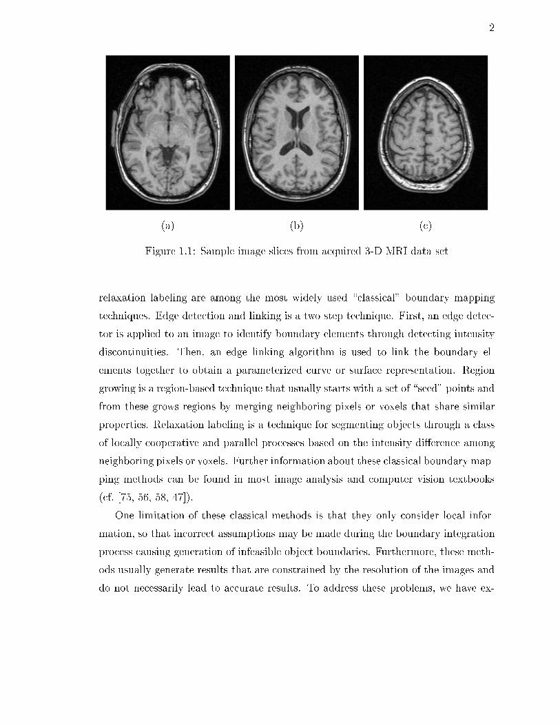
Mapping object boundaries from images is a diÆcult task due to the tremendous

variability of object shapes and diverse image sources. For example, one important

task in medical imaging is the boundary mapping of the brain cortex from 3-D mag-

netic resonance (MR) images (Fig. 1.1), where we are facing highly convoluted shape

of brain cortex, imaging noise, sampling artifacts, and large-scale image data set.

Imaging noise and sampling artifacts especially may cause the boundaries of objects

of interest to be indistinct and disconnected. How to integrate these boundaries into

a coherent and consistent mathematical description is a challenging problem that a

boundary mapping technique has to address.

Boundary mapping methods abound in the literature of image analysis, com-

puter vision, and medical imaging. Edge detection and linking, region growing, and

2

(a) (b) (c)

Figure 1.1: Sample image slices from acquired 3-D MRI data set

relaxation labeling are among the most widely used \classical" boundary mapping

techniques. Edge detection and linking is a two step technique. First, an edge detec-

tor is applied to an image to identify boundary elements through detecting intensity

discontinuities. Then, an edge linking algorithm is used to link the boundary el-

ements together to obtain a parameterized curve or surface representation. Region

growing is a region-based technique that usually starts with a set of \seed" points and

from these grows regions by merging neighboring pixels or voxels that share similar

properties. Relaxation labeling is a technique for segmenting objects through a class

of locally cooperative and parallel processes based on the intensity di�erence among

neighboring pixels or voxels. Further information about these classical boundary map-

ping methods can be found in most image analysis and computer vision textbooks

(cf. [75, 56, 58, 47]).

One limitation of these classical methods is that they only consider local infor-

mation, so that incorrect assumptions may be made during the boundary integration

process causing generation of infeasible object boundaries. Furthermore, these meth-

ods usually generate results that are constrained by the resolution of the images and

do not necessarily lead to accurate results. To address these problems, we have ex-

3

plored a boundary mapping technique called deformable models which is based on the

work of Kass et al. [62]. Various names have been used to refer deformable models

in the literature. In 2-D, deformable models are usually referred as snakes, active

contours, balloons, and deformable contours. In 3-D, they are usually referred as

active surfaces and deformable surfaces. In this thesis, we shall refer 2-D deformable

models as deformable contours and 3-D deformable models as deformable surfaces.

1.1 Deformable Models

Deformable models are elastic curves or surfaces de�ned within an image domain

that can move under the in uence of internal forces coming from within the curve or

surface itself and external forces computed from the image data. The internal and

external forces are de�ned so that the deformable model will conform to an object

boundary or other desired features within an image. Fig. 1.2 shows two examples of

using both a deformable contour and a deformable surface to reconstruct anatomical

boundaries from MR images. The results shown in this �gure are obtained using the

deformable models developed in this thesis.

Mathematically, deformable models are represented as parameterized manifolds

(curves or surfaces) x(u), where u is the parameter of the manifold. The shape of

the manifold is typically determined by a variational formulation whose general form

is the following: �nd the x(u) that minimize the energy functional

E = Eint + Eext =ZU

Eint(x(u)) +Eext(x(u)) du: (1.1)

This functional can be viewed as a representation of the energy of the manifold, and

the �nal shape of the manifold corresponds to the minimum of this energy. The

�rst term Eint prescribes a priori knowledge about the model such as its material

properties (elasticity and rigidity). It can be used to characterize the deformation of

a membrane or a thin-plate, for example. The second term Eext is usually derived

from image data and takes a minimum when the deformable model lies in the feature

of interest such as object boundary. More discussion about deformable models is

provided in Chapter 2.

4

(a) (b)

Figure 1.2: (a) A 2-D example of using a deformable contour to extract the inner wall

of the left ventricle of a human heart from an MR image. A sequence of deformablecontours (plotted in a shade of gray) and the �nal converged result (plotted in white).(b) A 3-D example of using a deformable surface to reconstruct the brain cortical

surface from a 3-D MR image.

1.2 Related Work

Although the name deformable models or snakes �rst appeared in work by Ter-

zopoulos and his collaborators [105, 62, 106, 108], the ideas of deforming an elastic

template date back much further to the work of Fischler and Elschlager's spring-

loaded templates [43] (1973) and Widrow's rubber mask technique [114] (1973). How-

ever, the popularity of deformable models to date is mostly credited to the work of

\Snakes" by Kass, Witkin, and Terzopoulos [62] (1987). Since the publication of

\Snakes", deformable models have grown to be one of the most active research areas

in the boundary mapping community. A complete review of deformable models is

beyond the scope of this thesis. Instead, we refer the interested readers to a survey

paper by McInerney and Terzopoulos [77]. Here, we shall only review work that is

needed to understand the methods developed in this thesis.

There are basically two types of deformable models discussed in the literature:

parametric deformable models (cf. [62, 5, 20, 76]) and geometric deformable models

5

(cf. [11, 73, 12, 113]). Geometric deformable models, based on the theory of curve

evolution and geometric ows [96, 63, 64, 3], represents curves and surfaces implicitly

as a level set of an evolving scalar function. Parametric deformable models, on the

other hand, represents curves and surfaces explicitly in its parametric forms. In this

thesis, we shall focus on parametric deformable models, although we expect our results

to have applications in geometric deformable models as well.

Parametric deformable models synthesize parametric curves or surfaces within

an image domain and allow them to move towards desired features, usually edges.

Typically, the model is drawn toward the edges by potential forces, which are de�ned

to be the negative gradient of a potential function. Additional forces, such as pressure

forces [20], together with the potential forces comprise the external forces. There are

also internal forces designed to hold the model together (elasticity forces) and to keep

it from bending excessively (bending forces).

There are two key diÆculties with parametric deformable models. First, the

initial model must, in general, be close to the true boundary or else it will likely

converge to the wrong result. Several methods have been proposed to address this

problem including multiresolution methods [68], pressure forces [20], and distance

potentials [21]. The basic idea is to increase the capture range of the external force

�elds and to guide the model toward the desired boundary. The second problem is

that deformable models have diÆculties progressing into boundary concavities [33, 1].

Although pressure forces [20], control points [33], domain-adaptivity [32], directional

attractions [1], and the use of solenoidal �elds [90] have been proposed, these methods

solve only one problem or both problems but with the price of creating new diÆculties.

For example, multiresolution methods have addressed the issue of capture range, but

specifying how the deformable model should move across di�erent resolutions remains

problematic. Another example is that of pressure forces, which can push a deformable

model into boundary concavities, but cannot be too strong or \weak" edges will be

overwhelmed [103]. Pressure forces must also be initialized to push out or push in, a

condition that mandates careful initialization.

One of the contributions of this thesis is the development of two new classes of

external force �elds derived from generalized vector di�usion equations that address

6

both problems listed above.

1.3 Brain Cortex Reconstruction

Our research on deformable models was motivated by one of the most interesting

and challenging problems in computational neuroanatomy: human cerebral cortex

reconstruction from MR images. This research is an important and fundamental

step in both image-guided neurosurgery [50, 110] and human brain mapping such

as brain geometry analysis [48, 59, 42, 91], functional mapping [27, 104, 41], spatial

normalization of brain images [102, 10, 29], and brain image registration [16, 22, 17, 30,

15]. Furthermore, extracted cortical surfaces can be used to study the morphological

variability of the brain in aging and among di�erent populations.

Geometrically, the human cerebral cortex is a thin folded sheet of gray matter

(GM) that lies inside the cerebrospinal uid (CSF) and outside the white matter

(WM) of the brain, as shown in Fig. 1.3. Reconstruction of the cortex from MR

images is problematic, however, due to diÆculties such as imaging noise, partial

volume averaging, image intensity inhomogeneities, convoluted cortical structures,

and the requirement to preserve anatomical topology. Preservation of topology is

important for morphometric analysis, surgical path planning, and functional mapping

where a representation consistent with anatomical structure is required.

Recently, there has been a considerable amount of work in this area of research.

Mangin et al. [74] and Teo et al. [104] reconstructed the cortex using a voxel-based

method. Volumetric registration proposed by Collins et al. [22] and Christensen

et al. [15] allows the generation of cortical surfaces from MR brain image volumes

given a template volume and its associated reconstructed cortical surface. Methods

of tracing 2-D contours either manually or automatically through 2-D image slices

followed by contour tiling to reconstruct the cortical surface have been described by

Drury et al. [42] and Klein et al. [65]. Dale & Sereno [27], MacDonald et al. [72],

Davatzikos & Bryan [31], and Sandor & Leahy [95] have used methods based on

deformable surface models to reconstruct cortical surfaces. The deformable surface

model is a suitable tool for cortical surface reconstruction due to its ability to deform

7

Ventricles

Ventricles

Sulcus

Gyrus

Gray matterWhite matter

CSF

Figure 1.3: A transaxial MR image of the human brain.

8

through a continuum and yield a continuous, smooth surface representation of the

cortex. Traditional deformable surface models, however, have diÆculties progressing

into convoluted regions resulting in reconstructed surfaces that lack the deep cortical

folds [74, 31, 95, 72].

In this thesis, we developed a systematic method for obtaining a parametric surface

representation of the central layer of the human cerebral cortex that addresses the

above diÆculties.

1.4 Thesis Contributions

Three main contributions are made in this thesis:

1. Gradient vector ow: A new deformable model formulation for boundary

mapping is developed. This new model uses a new type of external force called

gradient vector ow (GVF). The GVF external force has three advantages com-

pared to traditional external forces. First, it has a large capture range and allows

deformable models to be initialized far away from the object boundary. Second,

it can attract deformable models to move into boundary concavities where con-

ventional methods have diÆculties. Third, the GVF formulation is applicable

to any dimension allowing it to be applied in a wide range of applications. This

method is applied to both simulated images and real MR images.

2. Generalized gradient vector ow: Based on the GVF formulation, a gen-

eralization is developed to generate a family of vector �elds that share similar

properties as those of the GVF vector �eld. This generalization, called gen-

eralized gradient vector ow (GGVF), allows selection of external forces that

are superior to the GVF external forces for certain applications. An important

property called GGVF medialness, which results in an e�ective method for re-

constructing the central layer of thick boundaries, is introduced and analyzed.

We validate this method with both simulated and real MR images.

3. Brain cortex reconstruction: A new method based on the GGVF deformable

surfaces for reconstructing the human brain cortex is developed. Important ad-

9

vantages of this method over existing methods are that it reconstructs the entire

cortical surface including deep convoluted folds and that the reconstructed corti-

cal surface maintains the correct anatomical topology. This method is validated

on both phantom and real MR brain images. Next, a method for computing

di�erential geometry quantities on the reconstructed cortical surface and a pre-

liminary method for estimating the cortex thickness is developed. Finally, a

method that transforms the reconstructed cortical surface to a spherical map is

presented.

1.5 Previous Publications

Portions of this thesis have been previously published. The gradient vector ow

algorithm was published in [121, 123]. The generalized gradient vector ow algorithm

was published in [120, 122]. The brain cortex reconstruction method was published

in [118, 117, 119] and a journal version of this reconstruction technique has been

submitted as well [116]. The spherical mapping method was published in [115].

1.6 Thesis Organization

This thesis is organized as follows. In Chapter 2, we provide background materials

about deformable models. In Chapter 3, we develop the GVF deformable model. In

Chapter 4, we develop the GGVF deformable model, and study the medialness prop-

erty of GGVF vector �eld as well as the problem of central layer reconstruction of

thick boundaries. In Chapter 5, we develop the brain cortex reconstruction method

as well as methods for computing di�erential geometry quantities and mapping the

cortical surface to a sphere. Details of implementing deformable models and com-

puting di�erential geometry quantities can be found in thesis Appendices A and B.

Finally, we conclude the thesis in Chapter 6 with a summary and a discussion of

future research areas.

10

Chapter 2

Background

In this chapter, we provide a brief overview of traditional deformable contours

and surfaces. For each model, we start by introducing its variational formulation.

We then describe the commonly used external energy. Finally, we provide the solu-

tion to the variational formulation known as the Euler equation. Details of discrete

implementation are deferred to the end of this dissertation (Appendix A). A more

comprehensive treatment of deformable models can be found in [62, 21, 76].

2.1 Deformable Contours

A traditional deformable contour is a curve x(s) = [x(s); y(s)], s 2 [0; 1], that

moves through the spatial domain of an image to minimize the energy functional

E =Z 1

0

1

2(�jx0(s)j2 + �jx00(s)j2) + Eext(x(s))ds (2.1)

where � and � are weighting parameters that control the contour's tension and rigid-

ity, respectively, and x0(s) and x00(s) denote the �rst and second derivatives of x(s)

with respect to s. The external energy Eext is a function derived from the image

so that it takes on its smaller values at the features of interest, such as boundaries.

Given a gray-level image I(x; y), viewed as a function of continuous position variables

(x; y), typical external energies designed to lead a deformable contour toward step

11

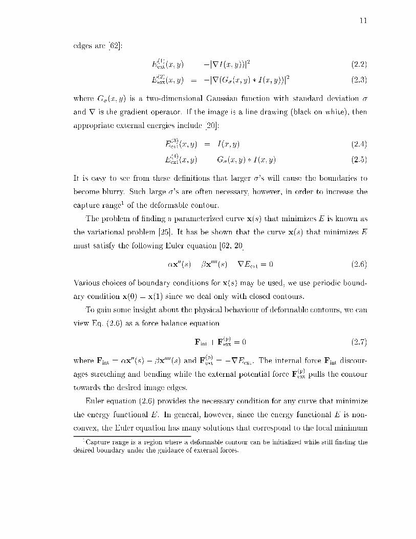
edges are [62]:

E(1)ext(x; y) = �jrI(x; y))j2 (2.2)

E(2)ext(x; y) = �jr(G�(x; y) � I(x; y))j2 (2.3)

where G�(x; y) is a two-dimensional Gaussian function with standard deviation �

and r is the gradient operator. If the image is a line drawing (black on white), then

appropriate external energies include [20]:

E(3)ext(x; y) = I(x; y) (2.4)

E(4)ext(x; y) = G�(x; y) � I(x; y) (2.5)

It is easy to see from these de�nitions that larger �'s will cause the boundaries to

become blurry. Such large �'s are often necessary, however, in order to increase the

capture range1 of the deformable contour.

The problem of �nding a parameterized curve x(s) that minimizes E is known as

the variational problem [25]. It has be shown that the curve x(s) that minimizes E

must satisfy the following Euler equation [62, 20]

�x00(s)� �x0000(s)�rEext = 0 (2.6)

Various choices of boundary conditions for x(s) may be used, we use periodic bound-

ary condition x(0) = x(1) since we deal only with closed contours.

To gain some insight about the physical behaviour of deformable contours, we can

view Eq. (2.6) as a force balance equation

Fint + F(p)ext = 0 (2.7)

where Fint = �x00(s) � �x0000(s) and F(p)ext = �rEext. The internal force Fint discour-

ages stretching and bending while the external potential force F(p)ext pulls the contour

towards the desired image edges.

Euler equation (2.6) provides the necessary condition for any curve that minimize

the energy functional E. In general, however, since the energy functional E is non-

convex, the Euler equation has many solutions that correspond to the local minimum

1Capture range is a region where a deformable contour can be initialized while still �nding the

desired boundary under the guidance of external forces.

12

of E [20, 19]. Although a global minimum can be found using several existing global

optimization techniques such as graduated non-convexity algorithms [8] and genetic

algorithms [34, 66], they are generally much more computational intensive than local

minimization techniques such as gradient descent methods. In this work, we will use

gradient descent methods to �nd the minimum. One of the consequence of using gra-

dient descent methods is that a good initialization is required to obtain a satisfactory

solution. This issue will be discussed in detail later in this thesis, and methods to

address this issue will be proposed as well. We note that the solution to the Euler

equation is assured to be a smooth curve that is at least twice-di�erentiable, as long

as either � or � is non-zero. Details on the mathematic properties of deformable

models can be found in [19].

To �nd a solution to (2.6), the deformable contour is made dynamic by treating

x as function of time t as well as s | i.e., x(s; t). We note that adding a time

directive term of x is equivalent to applying gradient descent algorithm to �nd the

local minimum of Eq. (2.1) [19]. Then, the partial derivative of x with respect to t is

then set equal to the left hand side of (2.6) as follows

xt(s; t) = �x00(s; t)� �x0000(s; t)�rEext (2.8)

When the solution x(s; t) stabilizes, the term xt(s; t) vanishes and we achieve a so-

lution of (2.6). A numerical solution to (2.8) can be found by discretizing the equa-

tion and solving the discrete system iteratively (cf. [62]). Details are provided in

Appendix A.1. We note that most deformable contour implementations use either a

parameter that multiplies xt in order to control the temporal step-size, or a parameter

that multiplies rEext, which permits separate control of the external force strength.

In this thesis, we normalize the external forces so that the maximum magnitude is

equal to one, and use a unit temporal step-size for all the experiments.

2.2 Deformable Surfaces

A traditional deformable surface is a surface x(u) = [x(u); y(u); z(u)], u =

(u1; u2) 2 [0; 1] � [0; 1], that moves through the spatial domain of a 3-D image to

13

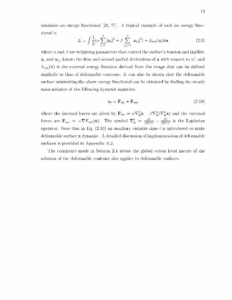
minimize an energy functional [21, 77]. A typical example of such an energy func-

tional is

E =Z1

2(�

2Xi=1

jxij2 + �2X

i;j=1

jxijj2) + Eext(x)du (2.9)

where � and � are weighting parameters that control the surface's tension and rigidity,

xi and xij denote the �rst and second partial derivatives of x with respect to ui, and

Eext(x) is the external energy function derived from the image that can be de�ned

similarly as that of deformable contours. It can also be shown that the deformable

surface minimizing the above energy functional can be obtained by �nding the steady

state solution of the following dynamic equation:

xt = Fint + Fext (2.10)

where the internal forces are given by Fint = �r2ux � �r2

u(r2

ux) and the external

forces are Fext = �rEext(x). The symbol r2u= @

2

(@u1)2+ @

2

(@u2)2is the Laplacian

operator. Note that in Eq. (2.10) an auxiliary variable time t is introduced to make

deformable surface x dynamic. A detailed discussion of implementation of deformable

surfaces is provided in Appendix A.2.

The comments made in Section 2.1 about the global versus local nature of the

solution of the deformable contours also applies to deformable surfaces.

14

Chapter 3

Gradient Vector Flow Deformable

Models

It is known that traditional deformable models have problems associated with

initialization and poor convergence to boundary concavities [83, 33, 1]. In this chap-

ter, we present a new class of external forces for deformable models that addresses

both problems listed above. These �elds, which we call gradient vector ow (GVF)

�elds, are dense vector �elds derived from images by minimizing a certain energy

functional in a variational framework. The minimization is achieved by solving a pair

of decoupled linear partial di�erential equations which di�uses the gradient vectors

of a gray-level or binary edge map computed from the image. We call the deformable

models that uses the GVF �eld as its external force a GVF deformable model. The

GVF deformable model is distinguished from nearly all previous deformable formu-

lations in that its external forces cannot be written as the negative gradient of a

potential function. Because of this, it cannot be formulated using the standard en-

ergy minimization framework; instead, it is speci�ed directly from a force balance

condition.

GVF can be de�ned in any dimension; however, in this chapter, we focus our

attention on two-dimensional problems for convenience. We shall refer 2-D deformable

models as deformable contours and those that use GVF as their external forces GVF

deformable contours. We note that all the discussions on GVF deformable contours

15

are valid to GVF deformable models in general. Accordingly, we show several 2-D

examples and one 3-D example at the end of the chapter.

Particular advantages of a GVF deformable contour over a traditional deformable

contour are its insensitivity to initialization and its ability to move into boundary

concavities. As we show in this chapter, its initializations can be inside, outside,

or across the object's boundary. Unlike the balloon model, the GVF deformable

contour does not need prior knowledge about whether to shrink or expand towards

the boundary. The GVF deformable contour also has a large capture range, which

means that, barring interference from other objects, it can be initialized far away

from the boundary. This increased capture range is achieved through a di�usion

process that does not blur the edges themselves, so multiresolution methods are not

needed. The external force model that is closest in spirit to GVF is the distance

potential forces of Cohen and Cohen [21]. Like GVF, these forces originate from an

edge map of the image and can provide a large capture range. We show, however,

that unlike GVF, distance potential forces cannot move a deformable contour into

boundary concavities. We believe that this is a property of all conservative forces

which characterize nearly all deformable contour external forces, and that exploring

non-conservative external forces, such as GVF, is an important direction for future

research in deformable contour models.

3.1 Behavior of Traditional Deformable Contours

An example of the behavior of a traditional deformable contour is shown in

Fig. 3.1. Fig. 3.1a shows a 64� 64-pixel line-drawing of a U-shaped object (shown in

gray) having a boundary concavity at the top. It also shows a sequence of curves (in

black) depicting the iterative progression of a traditional deformable contour (� = 0:6,

� = 0:0) initialized outside the object but within the capture range of the potential

force �eld. The potential force �eld F(p)ext = �rE(4)

ext (de�ned in Eq. (2.5)) where

� = 1:0 pixel is shown in Fig. 3.1b. We note that the �nal solution in Fig. 3.1a solves

the Euler equations of the deformable contour formulation, but remains split across

the concave region.

16

(a) (b)

(c)

Figure 3.1: (a) The convergence of a deformable contour using (b) traditional poten-

tial forces, (c) shown close-up within the boundary concavity.

17

The reason for the poor convergence of this deformable contour is revealed in

Fig. 3.1c, where a close-up of the external force �eld within the boundary concavity

is shown. Although the external forces correctly point toward the object boundary,

within the boundary concavity the forces point horizontally in opposite directions.

Therefore, the deformable contour is pulled apart toward each of the \�ngers" of the

U-shape, but not made to progress downward into the concavity. There is no choice

of � and � that will correct this problem.

Another key problem with traditional deformable contour formulations, the prob-

lem of limited capture range, can be understood by examining Fig. 3.1b. In this

�gure, we see that the magnitude of the external forces die out quite rapidly away

from the object boundary. Increasing � in (2.5) will increase this range, but the

boundary localization will become less accurate and distinct, ultimately obliterating

the concavity itself when � becomes too large.

Cohen and Cohen [21] proposed an external force model that signi�cantly increases

the capture range of a traditional deformable contour. These external forces are the

negative gradient of a potential function that is computed using a Euclidean (or cham-

fer) distance map. We refer to these forces as distance potential forces to distinguish

them from the traditional potential forces de�ned in Section 2.1. Fig. 3.2 shows the

performance of a deformable contour using distance potential forces. Fig. 3.2a shows

both the U-shaped object (in gray) and a sequence of contours (in black) depicting

the progression of the deformable contour from its initialization far from the object to

its �nal con�guration. The distance potential forces shown in Fig. 3.2b have vectors

with large magnitudes far away from the object, explaining why the capture range is

large for this external force model.

As shown in Fig. 3.2a, this deformable contour also fails to converge to the bound-

ary concavity. This can be explained by inspecting the magni�ed portion of the dis-

tance potential forces shown in Fig. 3.2c. We see that, like traditional potential forces,

these forces also point horizontally in opposite directions, which pulls the deformable

contour apart but not downward into the boundary concavity. We note that Cohen

and Cohen's modi�cation to the basic distance potential forces, which applies a non-

linear transformation to the distance map [21], does not change the direction of the

18

(a) (b)

(c)

Figure 3.2: (a) The convergence of a deformable contour using (b) distance potential

forces, (c) shown close-up within the boundary concavity.

19

forces, only their magnitudes. Therefore, the problem of convergence to boundary

concavities is not solved by distance potential forces.

3.2 Generalized Force Balance Equations

The deformable contour solutions shown in Figs. 3.1a and 3.2a both satisfy the

Euler equations (2.6) for their respective energy model. Accordingly, the poor �nal

con�gurations can be attributed to convergence to a local minimum of the objective

function (2.1). Several researchers have sought solutions to this problem by formulat-

ing deformable contours directly from a force balance equation in which the standard

external force F(p)ext is replaced by a more general external force F

(g)ext as follows

Fint + F(g)ext = 0 (3.1)

The choice of F(g)ext can have a profound impact on both the implementation and

the behavior of a deformable contour. Broadly speaking, the external forces F(g)ext

can be divided into two classes: static and dynamic. Static forces are those that

are computed from the image data, and do not change as the deformable contour

progresses. Standard deformable contour potential forces are static external forces.

Dynamic forces are those that change as the deformable contour deforms.

Several types of dynamic external forces have been invented to try to improve upon

the standard deformable contour potential forces. For example, the forces used in mul-

tiresolution deformable contours [68] and the pressure forces used in balloons [20] are

dynamic external forces. The use of multiresolution schemes and pressure forces, how-

ever, adds complexity to a deformable contour's implementation and unpredictability

to its performance. For example, pressure forces must be initialized to either push

out or push in, and may overwhelm weak boundaries if they act too strongly [103].

Conversely, they may not move into boundary concavities if they are pushing in the

wrong direction or act too weakly.

In this chapter, we present a new type of static external force, one that does not

change with time or depend on the position of the deformable contour itself. The un-

derlying mathematical premise for this new force comes from the Helmholtz theorem

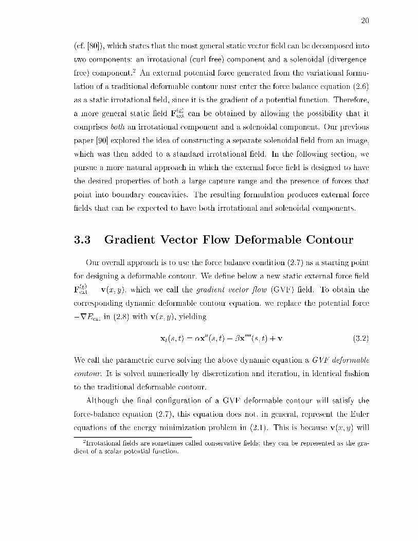
20

(cf. [80]), which states that the most general static vector �eld can be decomposed into

two components: an irrotational (curl-free) component and a solenoidal (divergence-

free) component.2 An external potential force generated from the variational formu-

lation of a traditional deformable contour must enter the force balance equation (2.6)

as a static irrotational �eld, since it is the gradient of a potential function. Therefore,

a more general static �eld F(g)ext can be obtained by allowing the possibility that it

comprises both an irrotational component and a solenoidal component. Our previous

paper [90] explored the idea of constructing a separate solenoidal �eld from an image,

which was then added to a standard irrotational �eld. In the following section, we

pursue a more natural approach in which the external force �eld is designed to have

the desired properties of both a large capture range and the presence of forces that

point into boundary concavities. The resulting formulation produces external force

�elds that can be expected to have both irrotational and solenoidal components.

3.3 Gradient Vector Flow Deformable Contour

Our overall approach is to use the force balance condition (2.7) as a starting point

for designing a deformable contour. We de�ne below a new static external force �eld

F(g)ext = v(x; y), which we call the gradient vector ow (GVF) �eld. To obtain the

corresponding dynamic deformable contour equation, we replace the potential force

�rEext in (2.8) with v(x; y), yielding

xt(s; t) = �x00(s; t)� �x0000(s; t) + v (3.2)

We call the parametric curve solving the above dynamic equation a GVF deformable

contour. It is solved numerically by discretization and iteration, in identical fashion

to the traditional deformable contour.

Although the �nal con�guration of a GVF deformable contour will satisfy the

force-balance equation (2.7), this equation does not, in general, represent the Euler

equations of the energy minimization problem in (2.1). This is because v(x; y) will

2Irrotational �elds are sometimes called conservative �elds; they can be represented as the gra-

dient of a scalar potential function.

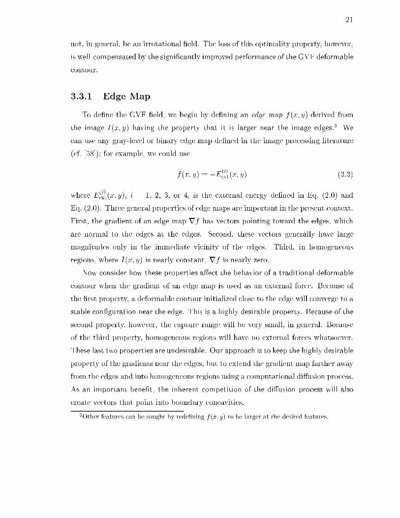
21

not, in general, be an irrotational �eld. The loss of this optimality property, however,

is well-compensated by the signi�cantly improved performance of the GVF deformable

contour.

3.3.1 Edge Map

To de�ne the GVF �eld, we begin by de�ning an edge map f(x; y) derived from

the image I(x; y) having the property that it is larger near the image edges.3 We

can use any gray-level or binary edge map de�ned in the image processing literature

(cf. [58]); for example, we could use

f(x; y) = �E(i)ext(x; y) (3.3)

where E(i)ext(x; y), i = 1, 2, 3, or 4, is the external energy de�ned in Eq. (2.0) and

Eq. (2.0). Three general properties of edge maps are important in the present context.

First, the gradient of an edge map rf has vectors pointing toward the edges, which

are normal to the edges at the edges. Second, these vectors generally have large

magnitudes only in the immediate vicinity of the edges. Third, in homogeneous

regions, where I(x; y) is nearly constant, rf is nearly zero.

Now consider how these properties a�ect the behavior of a traditional deformable

contour when the gradient of an edge map is used as an external force. Because of

the �rst property, a deformable contour initialized close to the edge will converge to a

stable con�guration near the edge. This is a highly desirable property. Because of the

second property, however, the capture range will be very small, in general. Because

of the third property, homogeneous regions will have no external forces whatsoever.

These last two properties are undesirable. Our approach is to keep the highly desirable

property of the gradients near the edges, but to extend the gradient map farther away

from the edges and into homogeneous regions using a computational di�usion process.

As an important bene�t, the inherent competition of the di�usion process will also

create vectors that point into boundary concavities.

3Other features can be sought by rede�ning f(x; y) to be larger at the desired features.

22

3.3.2 Gradient Vector Flow

We de�ne the gradient vector ow to be the vector �eld v(x; y) = [u(x; y); v(x; y)]

that minimizes the energy functional

E =Z Z

�(ux2 + uy

2 + vx2 + vy

2) + jrf j2jv�rf j2dxdy (3.4)

This variational formulation follows a standard principle, that of making the result

smooth when there is no data. In particular, we see that when jrf j is small, theenergy is dominated by sum of the squares of the partial derivatives of the vector

�eld, yielding a slowly-varying �eld. On the other hand, when jrf j is large, thesecond term dominates the integrand, and is minimized by setting v = rf . This

produces the desired e�ect of keeping v nearly equal to the gradient of the edge map

when it is large, but forcing the �eld to be slowly-varying in homogeneous regions.

The parameter � is a regularization parameter governing the tradeo� between the �rst

term and the second term in the integrand. This parameter should be set according

to the amount of noise present in the image (more noise, increase �).

We note that the smoothing term | the �rst term within the integrand of (3.4)

| is the same term used by Horn and Schunck in their classical formulation of optical

ow [57]. It has recently been shown that this term corresponds to an equal penalty

on the divergence and curl of the vector �eld [51]. Therefore, the vector �eld resulting

from this minimization can be expected to be neither entirely irrotational nor entirely

solenoidal.

Using the calculus of variations [25], it can be shown that the GVF �eld can be

found by solving the following Euler equations

�r2u� (u� fx)(fx2 + fy

2) = 0 (3.5a)

�r2v � (v � fy)(fx2 + fy

2) = 0 (3.5b)

where r2 is the Laplacian operator. These equations provide further intuition be-

hind the GVF formulation. We note that in a homogeneous region (where I(x; y) is

constant), the second term in each equation is zero because the gradient of f(x; y)

is zero. Therefore, within such a region, u and v are each determined by Laplace's

23

equation, and the resulting GVF �eld is interpolated from the region's boundary, re-

ecting a kind of competition among the boundary vectors. This explains why GVF

yields vectors that point into boundary concavities.

3.3.3 Numerical Implementation

Equations (3.5a) and (3.5b) can be solved by treating u and v as functions of time

and solving

ut(x; y; t) = �r2u(x; y; t)� (u(x; y; t)� fx(x; y))(fx(x; y)2 + fy(x; y)

2) (3.6a)

vt(x; y; t) = �r2v(x; y; t)� (v(x; y; t)� fy(x; y))(fx(x; y)2 + fy(x; y)

2) (3.6b)

The steady-state solution of these linear parabolic equations is the desired solution of

the Euler equations (3.5a) and (3.5b). Note that these equations are decoupled, and

therefore can be solved as separate scalar partial di�erential equations in u and v.

The equations in (3.6) are known as generalized di�usion equations, and are known

to arise in such diverse �elds as heat conduction, reactor physics, and uid ow [14].

Here, they have appeared from our description of desirable properties of deformable

contour external force �elds as represented in the energy functional of (3.4).

For convenience, we rewrite Equation (3.6) as follows

ut(x; y; t) = �r2u(x; y; t)� b(x; y)u(x; y; t) + c1(x; y) (3.7a)

vt(x; y; t) = �r2v(x; y; t)� b(x; y)v(x; y; t) + c2(x; y) (3.7b)

where

b(x; y) = fx(x; y)2 + fy(x; y)

2

c1(x; y) = b(x; y)fx(x; y)

c2(x; y) = b(x; y)fy(x; y)

Any digital image gradient operator (cf. [58]) can be used to calculate fx and fy. In

the examples shown in this paper, we use simple central di�erences. The coeÆcients

b(x; y), c1(x; y), and c2(x; y), can then be computed and �xed for the entire iterative

process.

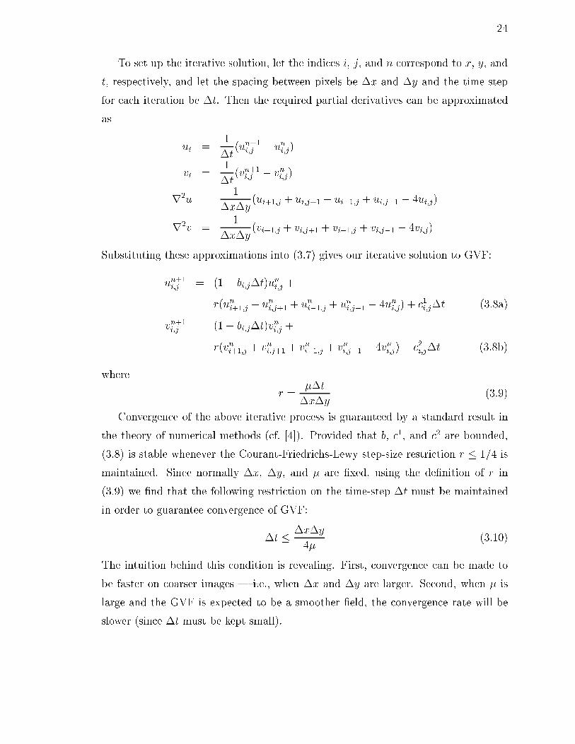
24

To set up the iterative solution, let the indices i, j, and n correspond to x, y, and

t, respectively, and let the spacing between pixels be �x and �y and the time step

for each iteration be �t. Then the required partial derivatives can be approximated

as

ut =1

�t(un+1

i;j� un

i;j)

vt =1

�t(vn+1

i;j� vn

i;j)

r2u =1

�x�y(ui+1;j + ui;j+1 + ui�1;j + ui;j�1 � 4ui;j)

r2v =1

�x�y(vi+1;j + vi;j+1 + vi�1;j + vi;j�1 � 4vi;j)

Substituting these approximations into (3.7) gives our iterative solution to GVF:

un+1i;j

= (1� bi;j�t)un

i;j+

r(uni+1;j + un

i;j+1 + uni�1;j + un

i;j�1 � 4uni;j) + c1

i;j�t (3.8a)

vn+1i;j

= (1� bi;j�t)vn

i;j+

r(vni+1;j + vn

i;j+1 + vni�1;j + vn

i;j�1 � 4vni;j) + c2

i;j�t (3.8b)

where

r =��t

�x�y(3.9)

Convergence of the above iterative process is guaranteed by a standard result in

the theory of numerical methods (cf. [4]). Provided that b, c1, and c2 are bounded,

(3.8) is stable whenever the Courant-Friedrichs-Lewy step-size restriction r � 1=4 is

maintained. Since normally �x, �y, and � are �xed, using the de�nition of r in

(3.9) we �nd that the following restriction on the time-step �t must be maintained

in order to guarantee convergence of GVF:

�t � �x�y

4�(3.10)

The intuition behind this condition is revealing. First, convergence can be made to

be faster on coarser images | i.e., when �x and �y are larger. Second, when � is

large and the GVF is expected to be a smoother �eld, the convergence rate will be

slower (since �t must be kept small).

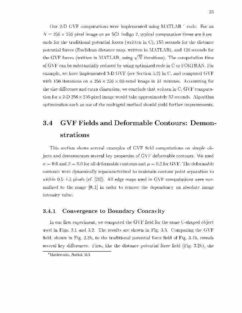
25

Our 2-D GVF computations were implemented using MATLAB 4 code. For an

N = 256� 256-pixel image on an SGI Indigo-2, typical computation times are 8 sec-

onds for the traditional potential forces (written in C), 155 seconds for the distance

potential forces (Euclidean distance map, written in MATLAB), and 420 seconds for

the GVF forces (written in MATLAB, usingpN iterations). The computation time

of GVF can be substantially reduced by using optimized code in C or FORTRAN. For

example, we have implemented 3-D GVF (see Section 5.2) in C, and computed GVF

with 150 iterations on a 256� 256� 60-voxel image in 31 minutes. Accounting for

the size di�erence and extra dimension, we conclude that written in C, GVF computa-

tion for a 2-D 256�256-pixel image would take approximately 53 seconds. Algorithm

optimization such as use of the multigrid method should yield further improvements.

3.4 GVF Fields and Deformable Contours: Demon-

strations

This section shows several examples of GVF �eld computations on simple ob-

jects and demonstrates several key properties of GVF deformable contours. We used

� = 0:6 and � = 0:0 for all deformable contours and � = 0:2 for GVF. The deformable

contours were dynamically reparameterized to maintain contour point separation to

within 0.5{1.5 pixels (cf. [70]). All edge maps used in GVF computations were nor-

malized to the range [0; 1] in order to remove the dependency on absolute image

intensity value.

3.4.1 Convergence to Boundary Concavity

In our �rst experiment, we computed the GVF �eld for the same U-shaped object

used in Figs. 3.1 and 3.2. The results are shown in Fig. 3.3. Comparing the GVF

�eld, shown in Fig. 3.3b, to the traditional potential force �eld of Fig. 3.1b, reveals

several key di�erences. First, like the distance potential force �eld (Fig. 3.2b), the

4Mathworks, Natick MA

26

(a) (b)

(c)

Figure 3.3: (a) The convergence of a deformable contour using (b) GVF external

forces, (c) shown close-up within the boundary concavity.

27

GVF �eld has a much larger capture range than traditional potential forces. A second

observation, which can be seen in the closeup of Fig. 3.3c, is that the GVF vectors

within the boundary concavity at the top of the U-shape have a downward component.

This stands in stark contrast to both the traditional potential forces of Fig. 3.1c and

the distance potential forces of Fig. 3.2c. Finally, it can be seen from Fig. 3.3b that

the GVF �eld behaves in an analogous fashion when viewed from the inside of the

object. In particular, the GVF vectors are pointing upward into the \�ngers" of the

U shape, which represent concavities from this perspective.

Fig. 3.3a shows the initialization, progression, and �nal con�guration of a GVF

deformable contour. The initialization is the same as that of Fig. 3.2a, and the

deformable contour parameters are the same as those in Figs. 3.1 and 3.2. Clearly,

the GVF deformable contour has a broad capture range and superior convergence

properties. The �nal deformable contour con�guration closely approximates the true

boundary, arriving at a sub-pixel interpolation through bilinear interpolation of the

GVF force �eld.

3.4.2 Streamlines

Streamlines are the paths over which free particles move when placed in an external

force �eld. By looking at their streamlines, we can examine the capture ranges and

motion inducing properties for various deformable contour external forces. Fig. 3.4

shows the streamlines of points arranged on a 32�32 grid for the traditional potentialforces, distance potential forces, and GVF forces used in the simulations of Figs. 3.1,

3.2, and 3.3.

Several properties can be observed from these �gures. First, the capture ranges of

the GVF force �eld and the distance potential force �eld are clearly much larger than

that of the traditional potential force �eld. In fact, both distance potential forces and

GVF forces will attract a deformable contour that is initialized on the image border.

Second, it is clear that GVF is the only force providing both a downward force within

the boundary concavity at the top of the U-shape and an upward force within the

\�ngers" of the U-shape. In contrast, both traditional deformable contour forces

28

(a) (b)

(c)

Figure 3.4: Streamlines originating from an array of 32�32 particles in (a) a tradi-

tional potential force �eld, (b) a distance potential force �eld, and (c) a GVF force

�eld.

29

and distance potential forces provide only sideways forces in these regions. Third,

the distance potential forces appear to have boundary points that act as regional

points of attraction. In contrast, the GVF forces attract points uniformly toward the

boundary.

3.4.3 Deformable Contour Initialization and Convergence

In this section we present several examples that compare di�erent deformable

contour models with the GVF deformable contour, showing various e�ects related to

initialization, boundary concavities, and subjective contours. The object under study

is the line drawing drawn in gray in both Figs. 3.5 and 3.6. This �gure may depict,

for example, the boundary of a room having two doors at the top and bottom and

two alcoves at the left and right. The open doors at the top and bottom represent

subjective contours that we desire to connect using the deformable contour (cf. [62]).

The deformable contour results shown in Figs. 3.5b{d all used the initialization

shown in Fig. 3.5a. We �rst note that for this initialization, the traditional potential

forces were too weak to overpower the deformable contour's internal forces, and the

deformable contour shrank to a point at the center of the �gure (result not shown).

To try to �x this problem, a balloon model with outward pressure forces just strong

enough to cause the deformable contour to expand into the boundary concavities

was implemented; this result is shown in Fig. 3.5b. Clearly, the pressure forces also

caused the balloon to bulge outward through the openings at the top and bottom,

and therefore the subjective contours are not reconstructed well.

The deformable contour result obtained using the distance potential force model

is shown in Fig. 3.5c. Clearly, the capture range is now adequate and the subjective

boundaries at the top and bottom are reconstructed well. But this deformable contour

fails to �nd the boundary concavities at the left and right, for the same reason that

it could not proceed into the top of the U-shaped object of the previous sections.

The GVF deformable contour result, shown in Fig. 3.5d, is clearly the best result. It

has reconstructed both the subjective boundaries and the boundary concavities quite

well. The slight rounding of corners, which can also be seen in Figs. 3.5b and 3.5c,

30

(a) (b)

(c) (d)

Figure 3.5: (a) An initial curve and deformable contour results from (b) a balloon

with an outward pressure, (c) a distance potential force deformable contour, and (d)a GVF deformable contour.

31

(a) (b)

(c) (d)

Figure 3.6: (a) An initial curve and deformable contour results from (b) a traditional

deformable contour, (c) a distance potential force deformable contour, and (d) a GVFdeformable contour.

32

is a fundamental characteristic of deformable contours caused by the regularization

coeÆcients � and �.5

The deformable contour results shown in Figs. 3.6b{d all used the initialization

shown in Fig. 3.6a, which is deliberately placed across the boundary. In this case,

the balloon model cannot be sensibly applied because it is not clear whether to apply

inward or outward pressure forces. Instead, the result of a deformable contour with

traditional potential forces is shown in Fig. 3.6b. This deformable contour stops at a

very undesirable con�guration because its only points of contact with the boundary

are normal to it and the remainder of the deformable contour is outside the capture

range of the other parts of the boundary. The deformable contour resulting from

distance potential forces is shown in Fig. 3.6c. This result shows that although the

distance potential force deformable contour possesses an insensitivity to initialization,

it is incapable of progressing into boundary concavities. The GVF deformable contour

result, shown in Fig. 3.6d, is again the best result. The GVF deformable contour

appears to have both an insensitivity to initialization and an ability to progress into

boundary concavities.

3.5 Gray-level Images and Higher Dimensions

In this section, we describe and demonstrate how GVF can be used in gray-level

imagery and in higher dimensions.

3.5.1 Gray-level Images

The underlying formulation of GVF is valid for gray-level images as well as bi-

nary images. To compute GVF for gray-level images, the edge-map function f(x; y)

must �rst be calculated. Two possibilities are f (1)(x; y) = jrI(x; y)j or f (2)(x; y) =jr(G�(x; y)� I(x; y))j, where the latter is more robust in the presence of noise. Othermore complicated noise-removal techniques such as median �ltering, morphological

�ltering, and anisotropic di�usion could also be used to improve the underlying edge

5The e�ect is only caused by � in this example since � = 0.

33

map. Given an edge-map function and an approximation to its gradient, GVF is

computed in the usual way using Eq. (3.8).

Fig. 3.7a shows a gray-level image of the U-shaped object corrupted by additive

white Gaussian noise; the signal-to-noise ratio is 6 dB. Fig. 3.7b shows an edge-

map computed using f(x; y) = f (2)(x; y) with � = 1:5 pixels, and Fig. 3.7c shows

the computed GVF �eld. It is evident that the stronger edge-map gradients are

retained while the weaker gradients are smoothed out, exactly as would be predicted

by the GVF energy formulation of (3.4). Superposed on the original image, Fig. 3.7d

shows a sequence of GVF deformable contours (plotted in a shade of gray) and the

GVF deformable contour result (plotted in white). The result shows an excellent

convergence to the boundary, despite the initialization from far away, the image noise,

and the boundary concavity.

Another demonstration of GVF applied to gray-scale imagery is shown in Fig. 3.8.

Fig. 3.8a shows a magnetic resonance image (short-axis section) of the left ventrical of

a human heart, and Fig. 3.8b shows an edge map computed using f(x; y) = f (2)(x; y)

with � = 2:5. Fig. 3.8c shows the computed GVF, and Fig. 3.8d shows a sequence

of GVF deformable contours (plotted in a shade of gray) and the GVF deformable

contour result (plotted in white), both overlaid on the original image. Clearly, many

details on the endocardial border are captured by the GVF deformable contour result,

including the papillary muscles (the bumps that protrude into the cavity).

3.5.2 Higher Dimensions

GVF can be easily generalized to higher dimensions. Let f(x) : ! R be an

edge map de�ned in � Rn. The GVF �eld in is de�ned as the vector �eld

v(x) : ! Rn that minimizes the energy functional

E =Z�jrvj2 + jrf j2 jv �rf j2dx (3.11)

where the gradient operator r is applied to each component of v separately. Using

the calculus of variations as described in Appendix 3.A, we �nd that the GVF �eld

34

(a) (b)

(c) (d)

Figure 3.7: (a) A noisy 64� 64-pixel image of a U-shaped object; (b) the edge mapjr(G� � I)j2 with � = 1:5; (c) the GVF external force �eld; and (d) convergence of

the GVF deformable contour.

35

(a) (b)

(c) (d)

Figure 3.8: (a) A 160� 160-pixel magnetic resonance image of the left ventrical of ahuman heart; (b) the edge map jr(G� � I)j2 with � = 2:5; (c) the GVF �eld (shown

subsampled by a factor of two); and (d) convergence of the GVF deformable contour.

36

must satisfy the Euler equation

�r2v � (v �rf)jrf j2 = 0 (3.12)

where r2 is also applied to each component of the vector �eld v separately.

A solution to these Euler equations can be found by introducing a time vari-

able t and �nding the steady-state solution of the following linear parabolic partial

di�erential equation

vt = �r2v � (v�rf)jrf j2 (3.13)

where vt denotes the partial derivative of v with respect to t. Equation (3.13) com-

prises n decoupled scalar linear second-order parabolic partial di�erential equations

in each element of v. Therefore, in principle, it can be solved in parallel. In analogous

fashion to the 2-D case, �nite di�erences can be used to approximate the required

derivatives and each scalar equation can be solved iteratively.

An experiment using GVF in three dimensions was carried out using the object

shown in Fig. 3.9a, which was created on a 643 grid, and rendered using an isosurface

algorithm. This object belongs to a family of closed surfaces calledmetaspheres which

is described in detail in Appendix 3.B. The 3-D GVF �eld was computed using a

numerical approximation to (3.13) and � = 0:15. This GVF result on the two planes

shown in Fig. 3.9b, is shown projected onto these planes in Figs. 3.9c and d. The

same characteristics observed in 2-D GVF �eld are apparent here as well.

Next, a deformable surface using 3-D GVF was initialized as the sphere shown in

Fig. 3.9e, which is neither entirely inside nor entirely outside the object. Intermediate

results after 10 and 40 iterations of the deformable surface algorithm are shown in

Figs. 3.9f and g. The �nal result after 100 iterations is shown in Fig. 3.9h. The

resulting surface is smoother than the isosurface rendering in Fig. 3.9a because of the

internal forces in the deformable surface model.

37

(a)

(b)

(c)

(d)

(e)

(f)

(g)

(h)

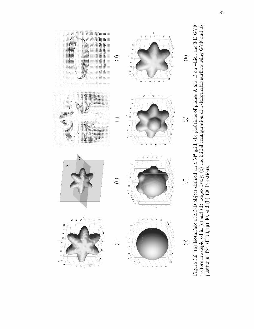
Figure3.9:(a)Isosurfaceofa3-Dobjectde�nedona643grid;(b)positionsofplanesAandBonwhichthe3-DGVF

vectorsaredepictedin(c)and(d),respectively;(e)theinitialcon�gurationofadeformablesurfaceusingGVFandits

positionsafter(f)10,(g)40,and(h)100iterations.

38

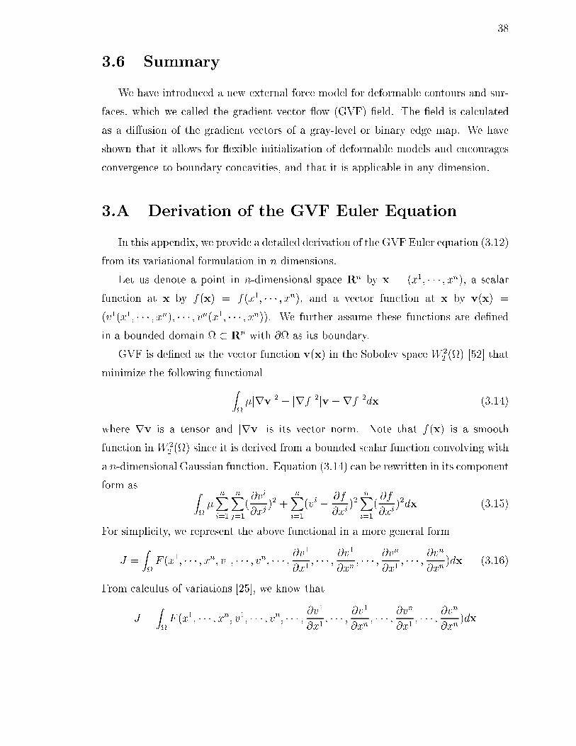
3.6 Summary

We have introduced a new external force model for deformable contours and sur-

faces, which we called the gradient vector ow (GVF) �eld. The �eld is calculated

as a di�usion of the gradient vectors of a gray-level or binary edge map. We have

shown that it allows for exible initialization of deformable models and encourages

convergence to boundary concavities, and that it is applicable in any dimension.

3.A Derivation of the GVF Euler Equation

In this appendix, we provide a detailed derivation of the GVF Euler equation (3.12)

from its variational formulation in n dimensions.

Let us denote a point in n-dimensional space Rn by x = (x1; � � � ; xn), a scalar

function at x by f(x) = f(x1; � � � ; xn), and a vector function at x by v(x) =

(v1(x1; � � � ; xn); � � � ; vn(x1; � � � ; xn)). We further assume these functions are de�ned

in a bounded domain � Rn with @ as its boundary.

GVF is de�ned as the vector function v(x) in the Sobolev space W 22 () [52] that

minimize the following functional

Z�jrvj2 + jrf j2jv �rf j2dx (3.14)

where rv is a tensor and jrvj is its vector norm. Note that f(x) is a smooth

function in W 22 () since it is derived from a bounded scalar function convolving with

a n-dimensional Gaussian function. Equation (3.14) can be rewritten in its component

form as Z�

nXi=1

nXj=1

(@vi

@xj)2 +

nXi=1

(vi � @f

@xi)2

nXi=1

(@f

@xi)2dx (3.15)

For simplicity, we represent the above functional in a more general form

J =ZF (x1; � � � ; xn; v1; � � � ; vn; � � � ; @v

1

@x1; � � � ; @v

1

@xn; � � � ; @v

n

@x1; � � � ; @v

n

@xn)dx (3.16)

From calculus of variations [25], we know that

J =ZF (x1; � � � ; xn; v1; � � � ; vn; � � � ; @v

1

@x1; � � � ; @v

1

@xn; � � � ; @v

n

@x1; � � � ; @v

n

@xn)dx

39

is stationary if and only if its �rst variation vanishes, i.e.,

ÆJ = 0 (3.17)

for every permissible variation Ævi 2 W 22 (), i = 1; � � � ; n.

By applying the laws of variation [54], we can then proceed to derive the stationary

solution to Eq. (3.17) as the following.

ÆJ = ÆZF (x1; � � � ; xn; v1; � � � ; vn; � � � ; @v

1

@x1; � � � ; @v

1

@xn; � � � ; @v

n

@x1; � � � ; @v

n

@xn)dx

=ZÆF (x1; � � � ; xn; v1; � � � ; vn; � � � ; @v

1

@x1; � � � ; @v

1

@xn; � � � ; @v

n

@x1; � � � ; @v

n

@xn)dx

=Z

24 nXi=1

@F

@viÆvi +

nXi=1

nXj=1

@F

@vij

Ævijdx

35 ; (vi � @vi

@xj)

=nXi=1

24Z

@F

@viÆvidx+

Z

nXj=1

@F

@vij

Ævijdx

35 :

Using integration by parts, we have

ÆJ =nXi=1

24Z

@F

@viÆvidx�

nXj=1

Z

@

@xj

@F

@vij

!Ævjdx+

nXj=1

Z@

@F

@vij

Ævi�idS

35

where �i is the projection of outward normal unit vector � along xi axis at @ and

dS represents the element of area on the boundary @. After rearranging the above

equation, we obtain

ÆJ =nXi=1

Z

24@F@vi

�nX

j=1

@

@xj

@F

@vij

!35 Ævjdx+ nX

i=1

nXj=1

Z@

@F

@vij

�iÆvidS = 0:

Since variations of Ævi, i = 1; � � � ; n are independent of each other, it follows that all

the coeÆcients of Ævi in the integrands of all the integrals must each vanish identically

in , giving n scalar Euler equations

@F

@vi�

nXj=1

@

@xj

@F

@vij

!= 0 (3.18)

and n natural boundary conditions

nXj=1

@F

@vij

�i = 0 (3.19)

40

where i = 1; � � � ; n. Substituting the de�nition of F in Eq. (3.15) and after some

algebra, we obtain the Euler equations and boundary conditions for GVF as follows:

�nX

j=1

@2vi

@(xj)2 �

vi � @f

@xj

! @f

@xj

!2

= 0 (3.20)

nXj=1

@vi

@xj�i = 0 on @ (3.21)

where i = 1; � � � ; n. Equation (3.20) and (3.21) can be written in a compact form

using the vector notation

�r2v � (v�rf)jrf j2 = 0 (3.22)

rv � � = 0 on @ (3.23)

This is a decoupled vector partial di�erential equation (PDE) with a Neumann bound-

ary condition. Each of its scalar equations is a linear, second-order, variable coeÆcient

PDE of the elliptic type. It has been shown that these scalar equations of GVF are

uniquely solvable [92, 26]6.

3.B Metaspheres

In this appendix, we describe a family of closed surfaces that can be used to

generate 3-D computational phantoms. These surfaces, which we call metaspheres,

are a generalization of basic harmonic curves given in [112].

Let us de�ne x = (x; y; z), a = (ax; ay; az), b = (bx; by; bz), m = (mx; my; mz),

and n = (nx; ny; nz). Then a metasphere x(�; �) is given by

x = (ax + bx cos(mx�) cos(nx�)) sin(�) cos(�) (3.24a)

y = (ay + by cos(my�) cos(ny�)) sin(�) sin(�) (3.24b)

z = (az + bz cos(mz�) cos(nz�)) cos(�) (3.24c)

where 0 � � < �, 0 � � < 2�, and (ax; ay; az) is the metasphere radius in the

directions of three axes, (bx; by; bz) is the ripple amplitude of harmonics components

6We would like to thank Diego Socolinsky for pointing out the references to the solvability of the

GVF Euler equation.

41

on the metasphere, and (mx; my; mz) and (nx; ny; nz) are the ripple frequencies. Three

examples of metasphere surfaces generated from Eq. (3.24) are shown in Figs. 3.10 a-c.

It is possible to bend the metasphere to add the variety of possible shape. A

metasphere that bends in x-y plane, ~x(�; �) = (~x; ~y; ~z), is given by

~x = x cos(cx) + y sin(cx) (3.25a)

~y = �x cos(cx) + y sin(cx) (3.25b)

~z = z (3.25c)

where c is a parameter that adjusts the amount of bending. Bending in other planes

is analogously de�ned. Fig. 3.10d shows a simple metasphere with bending.

42

(a) (b)

(c) (d)

Figure 3.10: Sample metaspheres: (a) a = (2; 2; 2), b = 0, m = 0, n = 0, and c = 0;

(b) a = (2; 2; 1), b = (0:5; 0:5; 0), m = 0, n = (6; 6; 6), and c = 0; (c) a = (2; 2; 2),

b = (0:5; 0:5; 0), m = (4; 4; 4), n = (4; 4; 4), and c = 0; and (d) a = (2; 0:5; 0:5),b = 0, m = 0, n = 0, and c = �0:4.

43

Chapter 4

Generalized Gradient Vector Flow

Deformable Models

In the previous chapter, we developed a new external force, called gradient vec-

tor ow (GVF), The GVF �eld has a large capture range, which means that the

deformable model can be initialized far away from the target boundary. The GVF

�eld also tends to force the deformable model into boundary concavities, where the

traditional deformable model have poor convergence. It still has diÆculties, however,

forcing a deformable model into long, thin boundary indentations, which is a crucial

requirement in applications such as brain cortex reconstruction.

In this chapter, we generalize the GVF formulation to include two spatially-varying

weighting functions. These weighting functions de�ne a tradeo� between smoothness

of the resulting GVF �eld and its conformity to the gradient of the underlying edge

map. The external force �elds derived from this new generalized GVF (GGVF) im-

prove the deformable model convergence into long, thin boundary indentations, while

maintaining other desirable properties of GVF, such as the extended capture range.

The original GVF is a special case of GGVF. In order to compare the performance

between GGVF deformable models and others, we performed a quantitative analysis

on a series of simulated test images and show the corresponding results.

In addition to being used as an external force �eld, GGVF can also be used as a

new type of image representation. In particular, it synthesizes a medial property of a

44

shape together with its boundary information. The medial property plays an impor-

tant role in shape analysis and computer vision and we shall describe a preliminary

study of medialness derived from the GGVF. An immediate application of GGVF

medialness is that we can use GGVF deformable models to reconstruct the central

layer of a thick boundary. Finally, we present an alternative generalization of GVF

through a variational formulation. This generalization satis�es a minimum principle

and results in similar performance as GGVF but requires more computations. We

note that all the GGVF formulas described in this chapter are presented in a vector

notation so that it can be used in any dimension, however, we give examples and

results in two-dimensional for convenience.

4.1 Generalized GVF

As was described in the previous chapter, GVF has many desirable properties

as an external force for deformable models. It still has diÆculties, however, forcing

a deformable model into long, thin boundary indentations. We hypothesized that

this diÆculty could be caused by excessive smoothing of the GVF �eld near the

boundaries, governed by the coeÆcient � in (3.13). We reasoned that introducing a

spatially-varying weighting function, instead of the constant �, and decreasing the

smoothing e�ect near strong gradients, could solve this problem. In the following

formulation, which we have termed generalized GVF (GGVF), we replace both � and

jrf j2 in (3.13) by more general weighting functions. An alternative generalization,

which follows from a variational formulation, is given in Section 4.5.

We de�ne GGVF as the equilibrium solution of the following vector partial di�er-

ential equation

vt = g(jrf j)r2v � h(jrf j)(v�rf) (4.1)

The �rst term on the right is referred to as the smoothing term since this term alone

will produce a smoothly varying vector �eld. The second term is referred as the data

term since it encourages the vector �eld v to be close to rf computed from the edge

map. The weighting functions g(�) and h(�) apply to the smoothing and data terms,

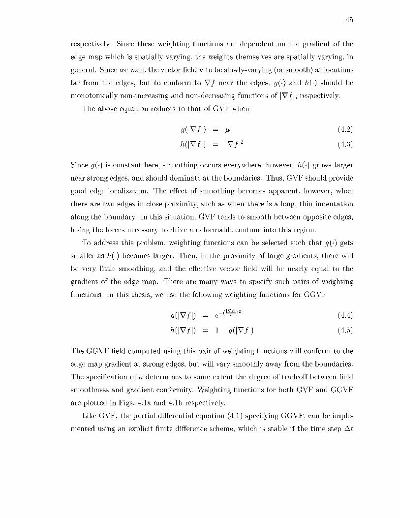
45

respectively. Since these weighting functions are dependent on the gradient of the

edge map which is spatially varying, the weights themselves are spatially varying, in

general. Since we want the vector �eld v to be slowly-varying (or smooth) at locations

far from the edges, but to conform to rf near the edges, g(�) and h(�) should be

monotonically non-increasing and non-decreasing functions of jrf j, respectively.The above equation reduces to that of GVF when

g(jrf j) = � (4.2)

h(jrf j) = jrf j2 (4.3)

Since g(�) is constant here, smoothing occurs everywhere; however, h(�) grows largernear strong edges, and should dominate at the boundaries. Thus, GVF should provide

good edge localization. The e�ect of smoothing becomes apparent, however, when

there are two edges in close proximity, such as when there is a long, thin indentation

along the boundary. In this situation, GVF tends to smooth between opposite edges,

losing the forces necessary to drive a deformable contour into this region.

To address this problem, weighting functions can be selected such that g(�) getssmaller as h(�) becomes larger. Then, in the proximity of large gradients, there will

be very little smoothing, and the e�ective vector �eld will be nearly equal to the

gradient of the edge map. There are many ways to specify such pairs of weighting

functions. In this thesis, we use the following weighting functions for GGVF

g(jrf j) = e�(jrf j�

)2 (4.4)

h(jrf j) = 1� g(jrf j) (4.5)

The GGVF �eld computed using this pair of weighting functions will conform to the

edge map gradient at strong edges, but will vary smoothly away from the boundaries.

The speci�cation of � determines to some extent the degree of tradeo� between �eld

smoothness and gradient conformity. Weighting functions for both GVF and GGVF

are plotted in Figs. 4.1a and 4.1b respectively.

Like GVF, the partial di�erential equation (4.1) specifying GGVF, can be imple-

mented using an explicit �nite di�erence scheme, which is stable if the time step �t

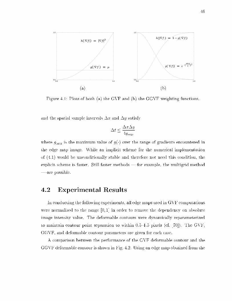
46

0.0 1.00.0

1.0

(a)

0.0 1.00.0

1.0

κ

(b)

Figure 4.1: Plots of both (a) the GVF and (b) the GGVF weighting functions.

and the spatial sample intervals �x and �y satisfy

�t � �x�y

4gmax

where gmax is the maximum value of g(�) over the range of gradients encountered in

the edge map image. While an implicit scheme for the numerical implementation

of (4.1) would be unconditionally stable and therefore not need this condition, the

explicit scheme is faster. Still faster methods | for example, the multigrid method

| are possible.

4.2 Experimental Results

In conducting the following experiments, all edge maps used in GVF computations

were normalized to the range [0; 1] in order to remove the dependency on absolute

image intensity value. The deformable contours were dynamically reparameterized

to maintain contour point separation to within 0.5{1.5 pixels (cf. [70]). The GVF,

GGVF, and deformable contour parameters are given for each case.

A comparison between the performance of the GVF deformable contour and the

GGVF deformable contour is shown in Fig. 4.2. Using an edge map obtained from the

47

(a) (b) (c)

(d) (e) (f)

Figure 4.2: (a) A square with a long, thin indentation and broken boundary; (b)

original GVF �eld (zoomed); (c) proposed GGVF �eld (zoomed); (d) initial contourposition for both the GVF deformable contour and the GGVF deformable contour;

(e) �nal result of the GVF deformable contour; and (f) �nal result of the GGVF

deformable contour.

48

original image shown in Fig. 4.2a, both the GVF �eld (� = 0:2) and the GGVF �eld

(� = 0:05) were computed, as shown zoomed in Figs. 4.2b and 4.2c, respectively. We

note that in this experiment both the GVF �eld and the GGVF �eld were normal-

ized with respect to their magnitudes and used as external forces. Next, a deformable

contour (� = 0:25, � = 0) was initialized at the position shown in Fig. 4.2d and al-

lowed to converge within each of the external force �elds. The GVF result, shown

in Fig. 4.2e, stops well short of convergence to the long, thin, boundary indentation.

On the other hand, the GGVF result, shown in Fig. 4.2f, is able to converge com-

pletely to this same region. It should be noted that both GVF and GGVF have wide

capture ranges (which is evident because the initial contour is fairly far away from

the object), and they both preserve subjective contours (meaning that they cross the

short boundary gaps).

It turns out that a good result similar to that of GGVF in Fig. 4.2f can be achieved

using GVF with � = 0:01. Because � is small in homogeneous regions as well as near

the edges, the convergence of GVF is very slow | it takes an order of magnitude

longer than GGVF or GVF with � = 0:2. If the GVF iterations are terminated early,

then the result has an undesirably small capture range. This result shows that GGVF

can be thought of as a faster GVF that preserves boundary detail and has a large

capture range. The GGVF and GVF results will never be exactly the same, however,

since the smoothing parameter of GGVF goes to zero at edges, an impossibility for

GVF.

We compared the accuracy of di�erent deformable contour formulations using the

simple harmonic curves. These curves were generated according to the equation

r = a + b cos(m� + c) (4.6)

by setting a, b, c to suitable values and varying m. Curves corresponding to m = 0,

2, 4, 6, and 8 were digitized on a 201 � 201 grid to give the images in Fig. 4.3. In

order to eliminate the problem of capture range for traditional deformable contours

so that comparisons could be made, we initialized the deformable contours at the true

curves, and let them deform under the di�erent external forces. After convergence, we

computed the maximum distance in the radial direction between the true boundary

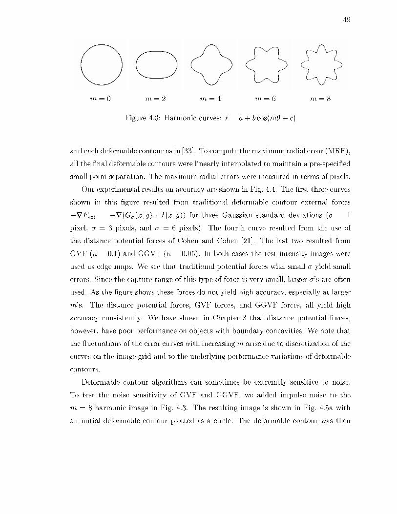
49

m = 0 m = 2 m = 4 m = 6 m = 8

Figure 4.3: Harmonic curves: r = a + b cos(m� + c)

and each deformable contour as in [33]. To compute the maximum radial error (MRE),

all the �nal deformable contours were linearly interpolated to maintain a pre-speci�ed

small point separation. The maximum radial errors were measured in terms of pixels.

Our experimental results on accuracy are shown in Fig. 4.4. The �rst three curves

shown in this �gure resulted from traditional deformable contour external forces

�rEext = �r(G�(x; y) � I(x; y)) for three Gaussian standard deviations (� = 1

pixel, � = 3 pixels, and � = 6 pixels). The fourth curve resulted from the use of

the distance potential forces of Cohen and Cohen [21]. The last two resulted from

GVF (� = 0:1) and GGVF (� = 0:05). In both cases the test intensity images were

used as edge maps. We see that traditional potential forces with small � yield small

errors. Since the capture range of this type of force is very small, larger �'s are often

used. As the �gure shows these forces do not yield high accuracy, especially at larger

m's. The distance potential forces, GVF forces, and GGVF forces, all yield high

accuracy consistently. We have shown in Chapter 3 that distance potential forces,

however, have poor performance on objects with boundary concavities. We note that

the uctuations of the error curves with increasingm arise due to discretization of the

curves on the image grid and to the underlying performance variations of deformable

contours.

Deformable contour algorithms can sometimes be extremely sensitive to noise.

To test the noise sensitivity of GVF and GGVF, we added impulse noise to the

m = 8 harmonic image in Fig. 4.3. The resulting image is shown in Fig. 4.5a with

an initial deformable contour plotted as a circle. The deformable contour was then

50

0 2 4 6 8m

0.0

0.5

1.0

1.5

2.0

Max

Err

or, p

ixel

σ = 1σ = 3σ = 6distanceGVFGGVF

Figure 4.4: Maximum radial error (MRE).

51

(a) (b) MRE = 49.0 (c) MRE = 7.2

(d) MRE = 52.3 (e) MRE = 2.3 (f) MRE = 2.2

Figure 4.5: (a) Impulse noise corrupted image and the initial deformable contour;(b) and (c) deformable contour results using traditional external forces r(G�(x; y) �I(x; y)) where � = 1 and 9; (d) deformable contour result using distance potentialforce; (e) GVF deformable contour result with � = 0:1; and (f) GGVF deformablecontour result with � = 0:2. The edge map used for both GVF and GGVF is f =

G�(x; y) � I(x; y), where � = 1, respectively. All deformable contour results are

computed using � = 0:25 and � = 0.

52

allowed to converge, being driven by external force �elds calculated from the noisy

image. The results for traditional deformable contours with � = 1 and � = 9 are

shown in Figs. 4.5b and 4.5c, respectively. The problem with Fig. 4.5b is that the

deformable contour is simply captured by the local impulsive spikes, rather than

the dominant �gure. In Fig. 4.5c, the large � blurs the boundary too much and

the deformable contour cannot latch onto the detail. The contour resulting from

the distance potential forces is shown in Fig. 4.5d. Since this external force uses a

binary edge map to begin with, it is attracted to the nearest detected edge points,

which do not belong to the dominant �gure. The results for both GVF and GGVF

deformable contours are shown in Figs. 4.5e and 4.5f, respectively. These results,

barely distinguishable from each other, demonstrate their abilities to be both captured

from a long distance and to converge extremely well to the dominant shape.

It is natural to ask whether there might be a smoothing strategy that would im-

prove the results of the distance potential forces. For example, it may be possible to

improve the edge map by pre�ltering the image before creating the edge map or by ap-

plying a nonlinear �lter to the edge map itself. We have tried several approaches along

these lines and have found that it is very diÆcult to eliminate extraneous boundary

points while simultaneously preserving the boundary itself. Another approach is to

�lter the distance potential itself in order to smooth out the energy valleys caused by

the extraneous edge points. This approach attens the valley in which the true edge is

located and does not eliminate the extraneous valleys, and the converged deformable

contour has poor �delity to the truth.

GVF and GGVF both improve over the distance potential forces by applying a

very narrow �lter to the edge map followed by a vector di�usion that allows the

dominant edge map to obliterate the e�ects of the extraneous edge points scattered

throughout the image. It should be noted that if GVF were run with a small � pa-

rameter, it would not smooth out the extraneous edges. This highlights an important

advantage of GGVF over GVF: that GGVF can support convergence to very thin

boundary concavities while simultaneously eliminating extraneous edge points.

Finally, we compared the qualitative performance of GVF and GGVF deformable

contours on a magnetic resonance image of the left ventricle of a human heart. The

53

original image is shown in Fig. 4.6a, and its gray-level edge map is shown in Fig. 4.6b.

The goal in this experiment is to extract the boundary description of the inner wall or

endocardium of the left ventricle. The initial positions of both GVF and GGVF de-

formable contours are shown as circles in gray overlaid on the real images (Figs. 4.6c

and 4.6d). The �nal contours are shown in white. Many details of the endocardial

border are captured by both GVF and GGVF; however, the papillary muscle pro-

truding into the cavity at about the 1 o'clock position is represented best by GGVF.

In many cases, GGVF and GVF will perform very similarly. Our experiments

have revealed certain di�erences, however, and these may be important in practice.

GGVF will generally show better convergence to thin boundary concavities. If the

� parameter is suÆciently small, however, GVF may achieve similar convergence

properties. But in this case, GVF will require signi�cantly longer computation time,

and noise in the edge map may cause erroneous convergence. In short, GGVF can

be thought of as a computationally faster version of GVF, with better boundary

localization, especially with respect to concave boundaries, and with better noise

immunity.

4.3 GGVF and Shape Analysis

In addition to its use as an external �eld for deformable models, GGVF appears

to have interesting connections to the medial axis analysis of shape. The medial axis

transform (MAT) [9] has long been used to describe both an object's shape and the

relationship among an object's natural parts [88]. The MAT representation is known

to be extremely sensitive to small boundary perturbations, however. To address

this diÆculty, Pizer et al. [87] introduced the multi-scale medial axis transform or

core which incorporates a scale space into the MAT by computing the maximum

medialness over scale. Medialness is a measure of how close a point is to an object's

skeleton. Because core analysis operates across scales, it reduces the noise sensitivity

of the MAT yet maintains almost all the desirable properties of MAT. In this section,

we show that by applying a simple algebraic transformation on the magnitude of a

GGVF �eld, we get a representation strongly resembling a medialness function.

54

(a) (b)

(c) (d)

Figure 4.6: (a) A 160� 160-pixel magnetic resonance image of the left ventrical of a

human heart; (b) the edge map jr(G�(x; y) � I(x; y))j2 with � = 2:5; (c) the result

of GVF deformable contour with � = 0:1; and (d) the result of GGVF deformablecontour with � = 0:15. The parameters used for both deformable contours are � = 0:1

and � = 0.

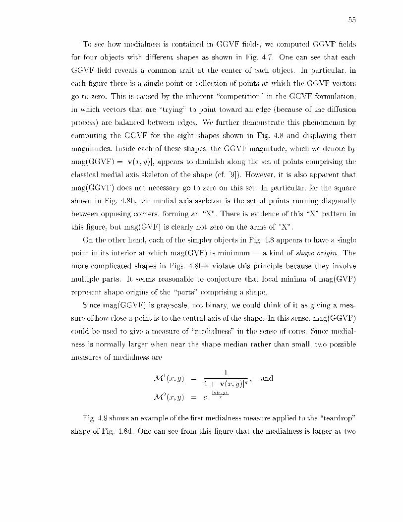
55

To see how medialness is contained in GGVF �elds, we computed GGVF �elds

for four objects with di�erent shapes as shown in Fig. 4.7. One can see that each

GGVF �eld reveals a common trait at the center of each object. In particular, in

each �gure there is a single point or collection of points at which the GGVF vectors

go to zero. This is caused by the inherent \competition" in the GGVF formulation,

in which vectors that are \trying" to point toward an edge (because of the di�usion

process) are balanced between edges. We further demonstrate this phenomenon by

computing the GGVF for the eight shapes shown in Fig. 4.8 and displaying their

magnitudes. Inside each of these shapes, the GGVF magnitude, which we denote by

mag(GGVF) = jv(x; y)j, appears to diminish along the set of points comprising the

classical medial axis skeleton of the shape (cf. [9]). However, it is also apparent that

mag(GGVF) does not necessary go to zero on this set. In particular, for the square

shown in Fig. 4.8b, the medial axis skeleton is the set of points running diagonally

between opposing corners, forming an \X". There is evidence of this \X" pattern in

this �gure, but mag(GVF) is clearly not zero on the arms of \X".

On the other hand, each of the simpler objects in Fig. 4.8 appears to have a single

point in its interior at which mag(GVF) is minimum | a kind of shape origin. The

more complicated shapes in Figs. 4.8f{h violate this principle because they involve

multiple parts. It seems reasonable to conjecture that local minima of mag(GVF)

represent shape origins of the \parts" comprising a shape.

Since mag(GGVF) is grayscale, not binary, we could think of it as giving a mea-

sure of how close a point is to the central axis of the shape. In this sense, mag(GGVF)

could be used to give a measure of \medialness" in the sense of cores. Since medial-

ness is normally larger when near the shape median rather than small, two possible

measures of medialness are

M1(x; y) =1

1 + jv(x; y)jq ; and

M2(x; y) = e�jv(x;y)j

�

Fig. 4.9 shows an example of the �rst medialness measure applied to the \teardrop"

shape of Fig. 4.8d. One can see from this �gure that the medialness is larger at two

56

(a) (b)

(c) (d)

Figure 4.7: GGVF �elds computed from objects with various shapes.

57

(a) (b)

(c) (d)

(e) (f)

(g) (h)

Figure 4.8: The magnitude of the GVF �eld gives information about the medial axis

of a shape.

58

(a) (b)

Figure 4.9: The medialness map M1(x; y) (q = 0:05) of a teardrop shape, shown as

(a) a gray-level image and (b) a surface plot.

other locations besides the skeleton, namely the object boundary and far outside

the object. It makes sense that medialness should be larger on the boundary since

the relevant shape near the boundary is the boundary itself. This observation will

prove to be useful in the next section where boundaries of certain thickness are con-

cerned. Also, as one moves farther away from the shape, the shape itself becomes

irrelevant, and every point should be medial. Therefore, it appears that the use of

mag(GGVF) has very strong potential use in shape analysis using medial axis ideas

and in particular to the concept of medialness in cores.

4.4 GGVF and the Central Layer of Thick Bound-

aries

The previous discussion on boundary mapping implicitly assumes boundaries in

images have negligible thickness. Boundaries of certain thickness, however, may also

occur either naturally in images such as the cortex of a brain or as a result of certain

59

Figure 4.10: GGVF vector �eld converges to the center of a thick edge.

boundary detection operations [28]. A natural way to represent such a thick boundary

is by reconstructing a curve or surface representation of its geometric central layer [28].

For example, Davatzikos and Prince have extracted central layers using deformable

models with a novel external force de�ned as the displacement from a deformable

model point to the center of image mass of a circular disk around this point [33]. One

limitation of this method is that boundaries with di�erent thicknesses require disks

with di�erent radii, prior knowledge that is not usually available.

Here, we show that it is possible use a GGVF deformable model to �nd central

layers accurately without any prior knowledge of the boundary thickness. As was

shown in the previous section, medialness de�ned through GGVF is larger on the

boundary. This observation can be made more precise by considering boundaries

with certain thickness. Fig. 4.10 shows an example of GGVF applied to a thick

boundary. One can see from this �gure that gradients at each side of the thick

boundary are di�used by GGVF towards the center layer of the thick boundary. The

vectors goes to zero at the center where the di�usion of gradients from both sides are

balanced. The GGVF di�usion process will lead GGVF vectors to converge to the

center regardless of the boundary thickness. This observation indicates that GGVF

deformable models can be used to reconstruct the central layer of thick boundaries,

as well as thin boundaries.

We demonstrate this property on simulated images (201 � 201) generated using

60

harmonic curves (Eq. (4.6)) corresponding to m = 0; 4; and 8 with thickness of 3,

6, and 9 pixels. Fig. 4.11 shows both the simulated images (in gray) and the recon-

structed central layers (in black) using GGVF deformable contours (� = 0:05; � = 0:1,

and � = 0). The maximum radial errors are computed for all the reconstructions.

Fig. 4.12 shows the maximum radial errors for the central layer reconstruction of

boundaries with di�erent thickness as a function of harmonic curves' frequency m.

We can make several observations from this plot. First, the overall maximum radial

error is around 12pixel except when m = 8 and thickness is 9 pixels where the error is

slightly larger than a pixel. Second, the errors increase as the boundary become more

convoluted. Further study to characterize the relationship among accuracy, curvature,

and thickness is warranted. Our primary interest in thick boundaries is motivated by

reconstructing the brain cortex with typical thickness range from 3 to 5 voxels. In

this application, GGVF deformable models are expected to work well. In Chapter 5,

we have a detailed error study on GGVF application to cortex reconstruction from

real MR brain images.

4.5 Variational Framework for Generalizing GVF

GVF can also be generalized by starting from its variational formulation Eq. (3.11)

introduced in Chapter 3. Spatially-varying weighting functions can be used, leading

to the following new variational formulation

E =Zg(jrf j)jrvj2 + h(jrf j)jv�rf j2dx

where j � j is a vector norm and rv is a second-order tensor. Using the calculus of

variations, we obtain the following Euler equation

r � [g(jrf j)rv]� h(jrf j)(v�rf) = 0

The solution of this vector equation can be obtained by computing the steady state

solution of the following generalized di�usion equation

vt = r � [g(jrf j)rv]� h(jrf j)(v�rf)

61

(a) m = 0 (b) m = 4 (c) m = 8

(d) m = 0 (e) m = 4 (f) m = 8

(g) m = 0 (h) m = 4 (i) m = 8

Figure 4.11: GGVF deformable contour results from simulated images with boundarythickness equal to 3 pixels (a)-(c), 6 pixels (d)-(f), and 9 pixels (g)-(i).

62

0 2 4 6 8m

0.0

0.5

1.0

1.5

Max

Err

or, p

ixel

thickness: 3 pixelsthickness: 6 pixelsthickness: 9 pixels

Figure 4.12: Maximum radial error for thick boundaries (MRE).

63

or written more explicitly

vt = rg(jrf j) � rv + g(jrf j)r2v � h(jrf j)(v�rf)

This result is di�erent than GGVF. To understand the nature of the di�erence,

we note that if rg(jrf j) � rv = 0, we get GGVF. This condition is data-dependent,

however, and is satis�ed in homogeneous regions, but is generally non-zero near the

edges. We have implemented this generalized GVF and found that it has very similar

properties as GGVF and usually yields a very similar result. This version is more

computationally demanding, however. Therefore, despite the aesthetically pleasing

property that it satis�es a minimum principle, we advocate GGVF when a general-

ization to GVF is desired.

4.6 Summary

We have presented a new class of external force models for deformable models.

It is a generalization of the GVF formulation that includes two spatially-varying

weighting functions. We showed that GGVF improves deformable model convergence

into long, thin boundary indentations and maintains other desirable properties of

GVF such as an extended capture range. We also showed that GGVF has excellent

performance on noisy and real medical images. In addition, the GGVF �eld was

shown to have potential applications in shape analysis, as well. The magnitude of the

�eld was shown to have information related to a shape's medial axis, and to the scale

space concept of medialness in the theory of cores. We have also shown that GGVF

deformable models can be used to reconstruct the central layers of thick boundaries.

Finally, we described an alternative approach to generalize the GVF by starting from

its variational formulation.

64

Chapter 5

Human Cerebral Cortex

Reconstruction from MR Images

In this chapter, we describe a systematic method for obtaining a parametric surface

representation of the central layer of the human cerebral cortex. The core component

of this method consists of an enhancement to the GGVF deformable models developed

in Chapter 4 by incorporating prior knowledge about brain anatomy. This method

also features a novel procedure to initialize deformable surfaces using an isosurface

algorithm. The deformable surface model is applied on membership functions com-

puted by an adaptive fuzzy segmentation rather than on image intensity volumes.

The resulting method is a largely automated method that reconstructs the entire

central cortical layer including deep convoluted sulci and gyri, while maintaining the

correct surface topology. Because of incorporating adaptive fuzzy segmentation in the

method, the method is robust to the partial volume averaging e�ects, image intensity

inhomogeneities, and raw image intensity variation across subjects.

This chapter is organized as follows. In Section 5.1, we describe our new cortical

surface reconstruction method. In Section 5.2, we present and discuss both qualitative

and quantitative results of applying our method to six di�erent subjects as well as

a simulated MR brain volume. In Section 5.3, we present some preliminary results

on brain geometry analysis. Finally, in Section 5.4, we summarize the results of this

chapter.

65

Raw MR images

Reconstructed cortical surface

1. Preprocessing

2. Fuzzy segmentation

3. GM/WM interface estimation

4. Deformable surface model

white matter

gray matter

initial surface

Figure 5.1: Block diagram of the overall cortical surface reconstruction system.

5.1 Methods

In this section, we present our method for reconstruction of the cortical surface

from MR brain image data. This method consists of four major steps. First, the

acquired data is preprocessed to extract the cerebrum and interpolated to cubic voxels.

Second, the brain image volume is segmented into fuzzy membership functions of GM,

WM, and CSF tissue classes using an adaptive segmentation algorithm that is robust

to image intensity inhomogeneities. Third, an iterative process of median �ltering and

isosurface generation on the WM membership function produces an initial estimate

of the cortical surface that is topologically correct. Fourth, our deformable surface

algorithm moves this surface toward the central layer of the cortex yielding the �nal

reconstructed cortical surface. Fig. 5.1 shows an overall ow diagram of our method.

Throughout this section, we use results from one subject as an example to illustrate

the method.

5.1.1 Data Acquisition and Preprocessing

Our algorithm uses T1-weighted volumetric MR image data with voxel size on the

order of 1 mm3. This data provides adequate contrast between gray matter, white

66

matter, and cerebrospinal uid in a single intensity parameter, and has �ne enough

resolution to resolve the complex structure of the cortex. It has been tested on both

axially acquired image data with in-plane resolution of 0.9375�0.9375 mm and out-

of-plane resolution of 1.5 mm and on coronal data with comparable resolution �gures.

The algorithm is easily modi�ed to use multi-spectral data, but the resolution must

be the same or better.

The �rst step in our method is to preprocess the image volume to remove skin,

bone, fat, and other non-cerebral tissue. We used a semi-automated software package

developed by Christos Davatzikos and Jerry Miller at Johns Hopkins University [46].

This package features a combination of region growing algorithms and mathematical

morphology operators to ease the processing of cerebral tissue extraction. It also

provides some manual editing features that were used to remove the cerebellum and

brain stem (since we are only interested in the cerebral cortex). We note that further

automation may be possible using the methods proposed in [94, 61, 67], but in our

experience some manual intervention was always required even with these approaches.

Fig. 5.3 shows the three slices from Fig. 5.2 after this procedure was applied.

The �nal step in preprocessing is to trilinearly interpolate the segmented volume

to cubic voxels having the in-plane resolution in all three directions. This reduces the

directional dependency in subsequent processing.

5.1.2 Fuzzy Segmentation of GM, WM and CSF

There has been a trend in the recent literature favoring the use of fuzzy seg-

mentations over hard segmentations in de�ning anatomical structures [13]. Fuzzy

segmentations retain more information from the original image than hard segmen-

tations by taking into account the possibility that more than one tissue class may

be present in a single voxel. This circumstance often occurs when imaging very �ne

structures, resulting in partial volume averaging. Small errors in the data acquisition

or segmentation will also be less of a factor in fuzzy segmentations since this will

only alter the segmentation by some fractional number while in a hard segmentation,

small errors might change the entire classi�cation of a voxel.

67

(a) (b)

(c)

Figure 5.2: Sample slices from acquired MRI data set.

68

(a) (b)

(c)

Figure 5.3: Sample slices after the cerebral tissue extraction.

69

MR images sometimes su�er from intensity inhomogeneities caused predominantly

by nonuniformities in the RF �eld during acquisition [23, 35]. The result is a slowly-

varying shading artifact appearing across images that can produce errors in intensity-

based segmentation methods. In particular, this artifact may cause the position of

the reconstructed cortex in various regions of the brain to be shifted slightly from

its true position. Robustness to intensity inhomogeneities is therefore an important

requirement in a cortical surface reconstruction algorithm.

Recently, Pham and Prince reported a new method called adaptive fuzzy c-means

(AFCM) [84, 85, 86] to obtain fuzzy segmentations of MR images that are robust to

intensity inhomogeneities. AFCM iteratively estimates the fuzzy membership func-

tions for each tissue class, the mean intensities (called centroids) of each class, and

the inhomogeneity of the image, modeled as a smoothly varying gain �eld. The fuzzy

membership functions, constrained to be between zero and one, re ect the degree of

similarity between the observed voxel intensity and the centroid of that tissue class.

A typical result from AFCM is shown in Fig. 5.4.

5.1.3 Estimation of Initial Surface with the Correct Topology

In order to use a deformable surface model to accurately reconstruct the extremely

convoluted cortical surface, a good initial surface is required. In the past, deformable

surfaces have been typically initialized using simple geometric objects (e.g., a sphere

or ellipsoid) outside the cortical surface or by manual interaction [72, 94, 42, 31].

When initialized from outside the cortical surface, however, deformable surfaces have

diÆculty progressing into the sulci [31]. As shown in Fig. 5.5, the primary diÆculty

with this approach is that sulci can be narrow relative to the resolution of the scanner,

so the imaged sulci become connected [74]. As a result, these deformable surfaces

produce cortical surface reconstructions that lack deep folds. Manual initializations

yield better results but they are labor intensive and time consuming for 3-D data

sets.

Because of the presence of WM, there is more space between the cortical folds

on the inside of the cortex than there is on the outside (see Fig. 5.5). Therefore,

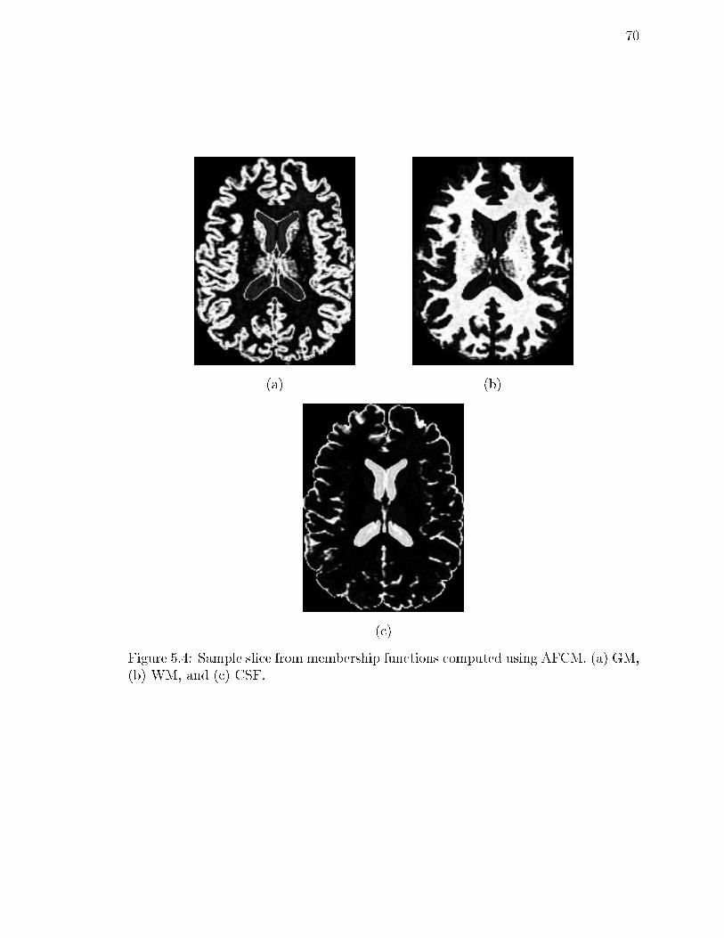
70

(a) (b)

(c)

Figure 5.4: Sample slice from membership functions computed using AFCM. (a) GM,(b) WM, and (c) CSF.

71

White Matter

Gray Matter CSF

(a)

White Matter

Gray Matter CSF

(b)

Figure 5.5: Resolution problems in determining the cortical surface. (a) ideal image,

and (b) sampled image.

initializing the deformable surface on the inside of the cortex is a promising strat-

egy [27, 118, 104]. Ideally, we desire an initial surface that is on the inside of the

cortex, is close to the �nal surface, and has the correct topology | that of a sphere.

As shown in Fig. 5.5, the GM-WM interface is both inside and close to the cortex. Ac-

cordingly, our approach is to �nd a surface that approximates the GM-WM interface

by �nding an isosurface of a �ltered WM membership function. Filtering is required

in order to make the initial surface have the correct topology. We now describe this

approach in detail.

Using an Isosurface Algorithm

An isosurface is a surface that passes through all locations in space where a

continuous data volume is equal to a constant value. The construction of isosurfaces

is a well-studied problem [71, 79, 60]. The result of a typical isosurface algorithm

usually consists of a set of triangle meshes that are discrete representations of the

corresponding continuous isosurfaces.

Since voxels at the GM-WM interface contain both GM and WM, an isosurface

can be computed on the WM membership function obtained from AFCM to yield an

estimate of the GM-WM interface. In order to use isosurfaces in the context of our

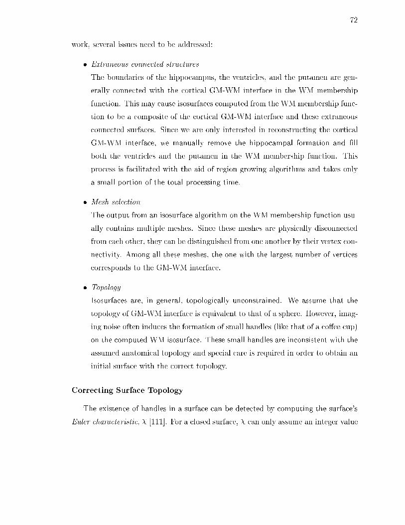
72

work, several issues need to be addressed:

� Extraneous connected structures

The boundaries of the hippocampus, the ventricles, and the putamen are gen-

erally connected with the cortical GM-WM interface in the WM membership

function. This may cause isosurfaces computed from the WM membership func-

tion to be a composite of the cortical GM-WM interface and these extraneous

connected surfaces. Since we are only interested in reconstructing the cortical

GM-WM interface, we manually remove the hippocampal formation and �ll

both the ventricles and the putamen in the WM membership function. This

process is facilitated with the aid of region growing algorithms and takes only

a small portion of the total processing time.

� Mesh selection

The output from an isosurface algorithm on the WM membership function usu-

ally contains multiple meshes. Since these meshes are physically disconnected

from each other, they can be distinguished from one another by their vertex con-

nectivity. Among all these meshes, the one with the largest number of vertices

corresponds to the GM-WM interface.

� Topology

Isosurfaces are, in general, topologically unconstrained. We assume that the

topology of GM-WM interface is equivalent to that of a sphere. However, imag-

ing noise often induces the formation of small handles (like that of a co�ee cup)

on the computed WM isosurface. These small handles are inconsistent with the

assumed anatomical topology and special care is required in order to obtain an

initial surface with the correct topology.

Correcting Surface Topology

The existence of handles in a surface can be detected by computing the surface's

Euler characteristic, � [111]. For a closed surface, � can only assume an integer value

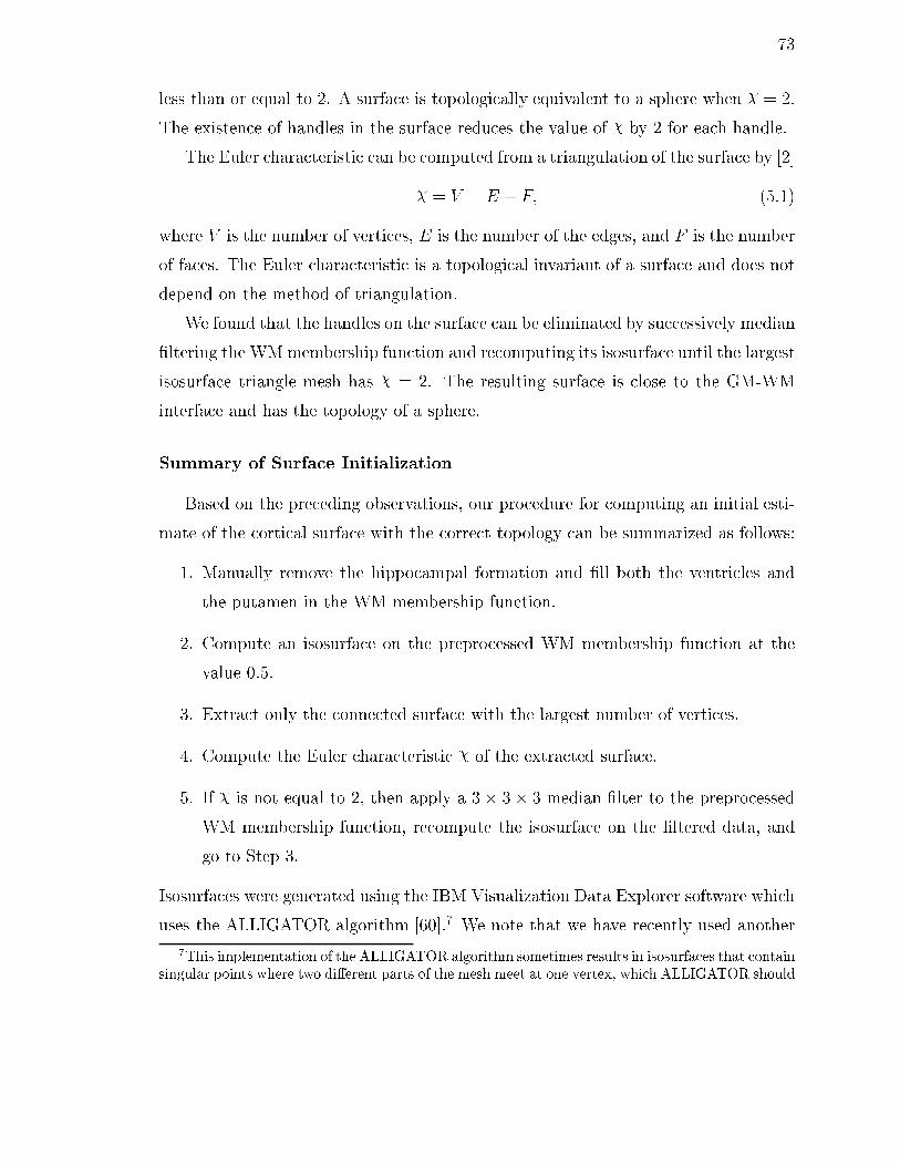
73

less than or equal to 2. A surface is topologically equivalent to a sphere when � = 2.

The existence of handles in the surface reduces the value of � by 2 for each handle.

The Euler characteristic can be computed from a triangulation of the surface by [2]

� = V � E + F; (5.1)

where V is the number of vertices, E is the number of the edges, and F is the number

of faces. The Euler characteristic is a topological invariant of a surface and does not

depend on the method of triangulation.

We found that the handles on the surface can be eliminated by successively median

�ltering the WMmembership function and recomputing its isosurface until the largest

isosurface triangle mesh has � = 2. The resulting surface is close to the GM-WM

interface and has the topology of a sphere.

Summary of Surface Initialization

Based on the preceding observations, our procedure for computing an initial esti-

mate of the cortical surface with the correct topology can be summarized as follows:

1. Manually remove the hippocampal formation and �ll both the ventricles and

the putamen in the WM membership function.

2. Compute an isosurface on the preprocessed WM membership function at the

value 0.5.

3. Extract only the connected surface with the largest number of vertices.

4. Compute the Euler characteristic � of the extracted surface.

5. If � is not equal to 2, then apply a 3� 3� 3 median �lter to the preprocessed

WM membership function, recompute the isosurface on the �ltered data, and

go to Step 3.

Isosurfaces were generated using the IBM Visualization Data Explorer software which

uses the ALLIGATOR algorithm [60].7 We note that we have recently used another

7This implementation of the ALLIGATOR algorithm sometimes results in isosurfaces that contain

singular points where two di�erent parts of the mesh meet at one vertex, which ALLIGATOR should

74

Table 5.1: Size and Euler characteris-

tics of meshes from the original isosurface

calculation.

# of vertices � # of meshes

360,104 �1010 1

506 �6 1

250 { 499 2 1100 { 249 2 11

50 { 99 2 28

25 { 49 2 97

6 { 24 2 1970

Table 5.2: Euler characteristic of

largest resulting surface after each

iteration.

# of iterations �

0 �10101 �562 �143 �4

4 { 7 �28 0

9 2

isosurface algorithm from Visualization Toolkit software [97] and obtained identical

results. Except for Step 1, all of the steps are performed automatically.

A typical result of applying the above procedure to one of our data sets is shown

in Tables 5.1 and 5.2, and Fig. 5.6. Table 5.1 shows the number of meshes and their

� values before any median �ltering has taken place. The one mesh that is clearly

much larger than all other meshes represents an estimate of the GM-WM interface

with an incorrect topology. Table 5.2 shows how the � of the largest resulting mesh

is increasing with each iteration and eventually converges to the desired value of 2.

Although there is no theoretical proof that successive median �ltering will cause the

Euler characteristic to converge to 2, we have found empirically that this is the case.

Experimental results on the convergence of the deformable surface initialization are

provided in Section 5.2.2.

Fig. 5.6a shows the result of the isosurface algorithm on the original WM mem-

bership function at a value of 0.5. Multiple meshes and topological inconsistencies are

present. Fig. 5.6b shows the �nal, topologically correct mesh after nine iterations of

our procedure. We see that although we have not yet applied the deformable surface

model, many of the prominent geometrical characteristics of this cortical surface are

prohibit. In this case, methods to remove singular points were also incorporated into the iterative

procedure.

75

(a)

(b)

Figure 5.6: (a) Isosurface of WM membership function with the incorrect topology,

(b) estimated initial surface with the correct topology.

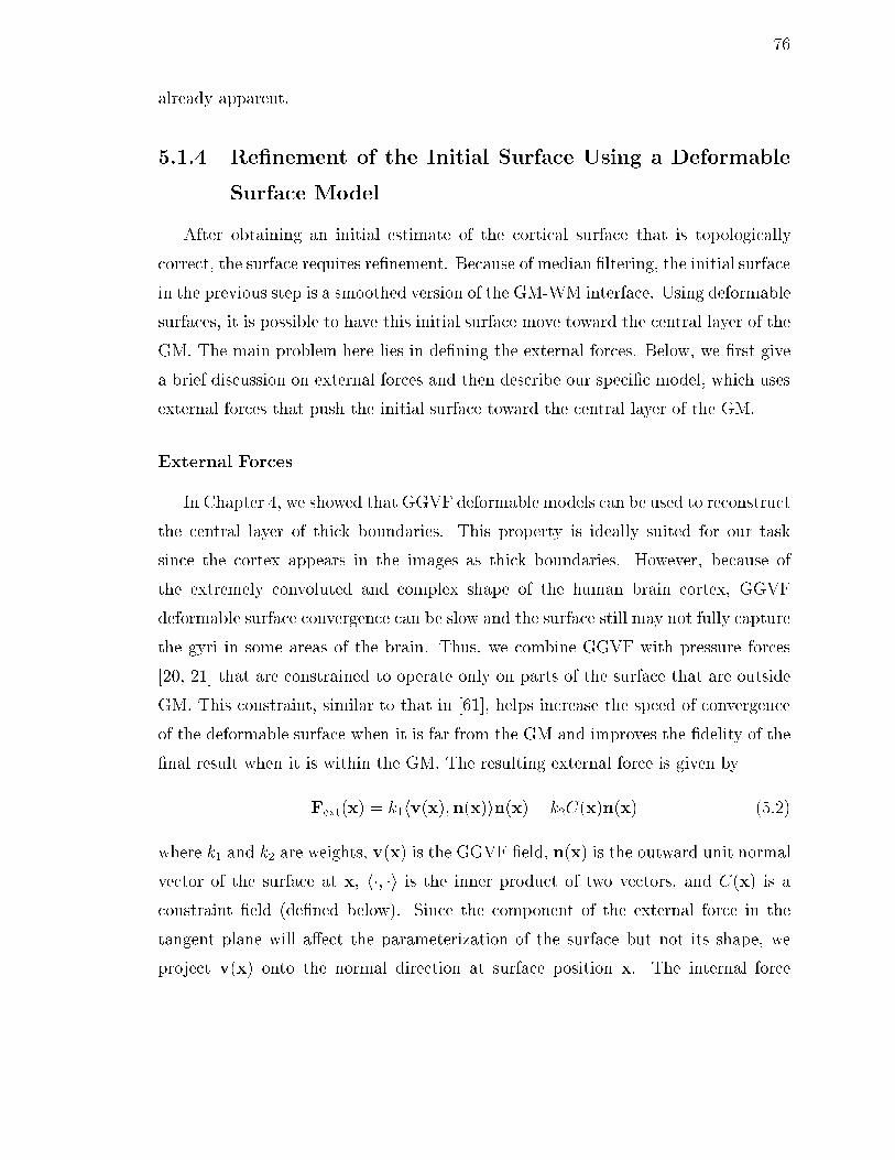
76

already apparent.

5.1.4 Re�nement of the Initial Surface Using a Deformable

Surface Model

After obtaining an initial estimate of the cortical surface that is topologically

correct, the surface requires re�nement. Because of median �ltering, the initial surface

in the previous step is a smoothed version of the GM-WM interface. Using deformable

surfaces, it is possible to have this initial surface move toward the central layer of the

GM. The main problem here lies in de�ning the external forces. Below, we �rst give

a brief discussion on external forces and then describe our speci�c model, which uses

external forces that push the initial surface toward the central layer of the GM.

External Forces

In Chapter 4, we showed that GGVF deformable models can be used to reconstruct

the central layer of thick boundaries. This property is ideally suited for our task

since the cortex appears in the images as thick boundaries. However, because of

the extremely convoluted and complex shape of the human brain cortex, GGVF

deformable surface convergence can be slow and the surface still may not fully capture

the gyri in some areas of the brain. Thus, we combine GGVF with pressure forces

[20, 21] that are constrained to operate only on parts of the surface that are outside

GM. This constraint, similar to that in [61], helps increase the speed of convergence

of the deformable surface when it is far from the GM and improves the �delity of the

�nal result when it is within the GM. The resulting external force is given by

Fext(x) = k1hv(x);n(x)in(x) + k2C(x)n(x) (5.2)

where k1 and k2 are weights, v(x) is the GGVF �eld, n(x) is the outward unit normal

vector of the surface at x, h�; �i is the inner product of two vectors, and C(x) is a

constraint �eld (de�ned below). Since the component of the external force in the

tangent plane will a�ect the parameterization of the surface but not its shape, we

project v(x) onto the normal direction at surface position x. The internal force

77

x

uwm(x) ugm(x)

C(x)

x

δ

Figure 5.7: Illustration of behavior of C(x).

is therefore solely responsible for controlling the surface parameterization while the

external force is solely responsible for deforming the surface toward the feature of

interest.

The constrained pressure force C(x)n(x) is designed to push the surface outward

only until it enters the GM, whereupon the pressure force then turns o� and GGVF

completes the convergence. To accomplish this, we de�ne the strength of the pressure

force, as controlled by the constraint �eld C(x), to be

C(x) =

8<:

0 if j2 � uwm(x) + ugm(x)� 1j < Æ

2 � uwm(x) + ugm(x)� 1 otherwise

where uwm(x) and ugm(x) are the WM and GM membership functions. Here, Æ is

a threshold that controls the width of the GM region where the pressure force is

disabled, i.e. C(x) = 0. In our experiments we used Æ = 0:5. The behavior of C(x)

is illustrated in Fig. 5.7 where one-dimensional pro�les of GM and WM membership

functions and the corresponding C(x) are plotted. It is easy to see that when x is

in the WM, C(x) is positive, which causes the pressure force to push a deformable

surface towards the GM. When x is in the GM, C(x) is zero and the GGVF force is

the only external force. When x is outside the GM in the CSF or background, C(x)

is negative, causing the pressure force to push the deformable surface back toward

78

Figure 5.8: Initial deformable contour shown in black and �nal converged contourshown in white.

the GM.

To demonstrate the behavior of these external forces, we applied a 2-D deformable

contour, a 2-D analog to deformable surfaces in 3-D, using the external forces de�ned

in Eq. (5.2) to the computer phantom shown in Fig. 5.8. Here, the gray ribbon is

analogous to the cortical GM, sandwiched between the WM and the CSF. In the

�gure, the initial deformable contour is the circle shown in black, while the �nal

converged contour is shown in white. We note that the �nal contour rests on the

center of the simulated GM.

Adaptive Parameters

Because of image noise, relatively large internal forces are desirable where the

deformable surface is far from the GM. Large internal forces cause the deformable

surfaces to be very smooth, however, and prevent the surface from accurately con-

forming to the central cortical layer. Therefore, lower internal forces are desirable

where the deformable surface lies within the GM. We achieve this by allowing � and

� to be spatially varying parameters in Eq. (2.9) with respect to the strength of the

79

constraint �eld C(x) as follows

�(x) =

8<:

� if jC(x)j = 0

�� otherwise;

and

�(x) =

8<:

� if jC(x)j = 0

�� otherwise

where �� � � and �� � �.

5.1.5 Reconstructed Surface

As an example, we carried out the complete surface reconstruction on the sample

data set appearing in Figs. 5.2, 5.3, 5.4, and 5.6. Di�erent views of the reconstructed

surface are shown in Fig. 5.9, and cross sectional views are shown in Fig. 5.10. The

parameters used to achieve this result are �1 = 2� 104 and �2 = 2� 105 for AFCM;

� = 0:2 for GGVF; and � = 0:25, � = 0, �� = 0:75, �� = 0, k1 = 0:5, and k2 = 0:01 for

the deformable surface. While this may appear to be a large number of parameters

to tune, we have found that they are fairly robust to both changes in their values and

the data. In fact, all the results presented in the following section use these same

parameters.

At �rst glance, the sulci in the surface shown in Fig. 5.9 appear too open and

do not resemble those from a normal brain. Note, however, that this reconstruction

represents the central layer of the cortical GM, an object that we are not accustomed

to viewing. The central layer is not the brain's outer surface such as what would

be seen from a cadaver brain or a standard isosurface reconstruction of the cortical

surface. Careful inspection reveals exquisite depiction of the major sulci including the

central sulci, superior temporal sulci, calcarine sulci, parietal occipital sulci, and the

Sylvian �ssure. Secondary sulci such as the pre- and post- central sulci, the superior

frontal sulci, and the cingulate sulci are also readily discernible. Their prominence in

these pictures is to some extent because we are depicting a more open brain surface,

but also because the central cortical layer is the most natural representation of the

overall geometry of the cortex.

80

(a) (b)

(c) (d)

(e) (f)

Figure 5.9: A surface rendering of reconstructed cortical surface from one subject

displayed from multiple views: (a) top, (b) bottom, (c) left, (d) right, (e) left medial,and (f) right medial.

81

(a) (b) (c)

Figure 5.10: Cross sectional views of the reconstructed cortical surface: (a) axial, (b)

coronal, and (c) sagittal.

The cross sectional pictures in Fig. 5.10 show how the reconstructed surface tracks

the central cortical layer over the entire cortex, including its deepest folds. In fact,

because the surface is initialized inside the cortex, the most diÆcult areas to recon-

struct are typically the gyri, not the sulci. A typically diÆcult area is the superior

temporal gyri, which is not particularly well-reconstructed on the left side of the pic-

ture in Fig. 5.10b. Other features of interest appearing on these cross-sections are the

various \islands" of apparently disconnected surface intersections. These features are

actually parts of the surface protruding through the image plane; the surface being

portrayed is simply-connected with the topology of a sphere.

5.2 Results

We applied the described cortical surface reconstruction method to MR brain

images from six subjects, four of which were taken from the Baltimore Longitudinal

Study on Aging [99]. The same parameters used in the example from the previous

section were used for these six studies. Using an SGI O2 workstation with a 174 MHz

R10000 processor, the total processing time per study varied between 4.5 and 6 hours.

The time required for manual interaction varied between 0.5 hours and 1 hour for a

trained operator and AFCM required approximately 1 hour. The automated steps

82

in GM/WM interface estimation take about 0.5 hours and produce a mesh with

between 200,000 and 400,000 vertices. Because of the large number of vertices in the

mesh, it takes the deformable surface algorithm about 3 hours to produce the �nal

reconstructed surface. Note that both AFCM and the deformable surface algorithm

are fully automated steps.

5.2.1 Qualitative Results

Fig. 5.11 shows the right medial surface of each of the six reconstructed cortical

surfaces. Prominent sulci include the calcarine �ssure, the parieto-occipital sulcus,

and the cingulate sulcus. Fig. 5.12 shows a coronal view of a slice taken approximately

at the anterior commissure of each reconstructed cortical surface. These �gures show

that the surfaces reside on the central cortical layer and that buried gyri (such as the

insula) are found. Although most gyri are properly depicted, certain regions, such as

the superior temporal gyrus, are sometimes not found accurately. This is particularly

apparent in Figs. 5.12e and 5.12f. We are considering further improvements to correct

these de�ciencies.

5.2.2 Quantitative Results

Several quantitative validation experiments were performed to evaluate the ro-

bustness and accuracy of our surface reconstruction approach. These are described

in this section.

Initialization Algorithm Validation

Application of our method to multiple subjects allowed a preliminary validation

of the convergence of the deformable surface initialization algorithm introduced in

Section 5.1.3. The results are shown in Table 5.3, where we observe that the median

�lter used in the iterative process e�ectively eliminates handles on the surfaces, and

that in all six cases the Euler characteristic of the surface converged to 2 in fewer

than 10 iterations.

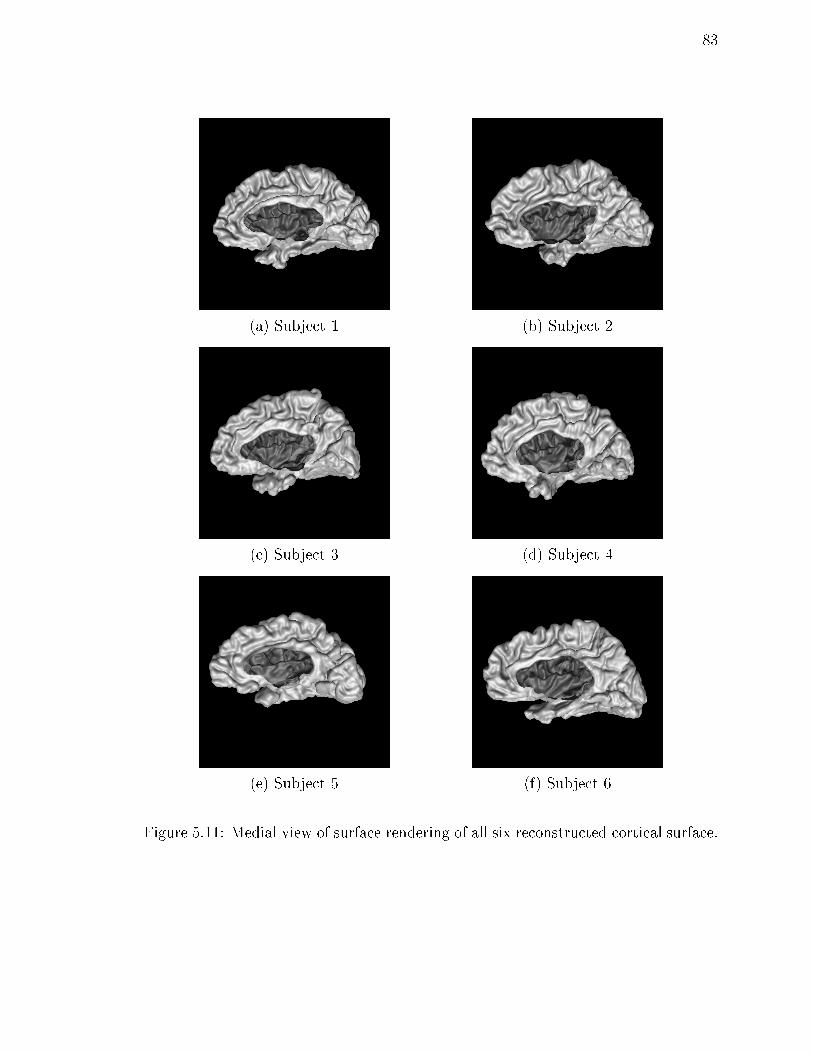
83

(a) Subject 1 (b) Subject 2

(c) Subject 3 (d) Subject 4

(e) Subject 5 (f) Subject 6

Figure 5.11: Medial view of surface rendering of all six reconstructed cortical surface.

84

(a) Subject 1 (b) Subject 2

(c) Subject 3 (d) Subject 4

(e) Subject 5 (f) Subject 6

Figure 5.12: From left to right and top to bottom, the coronal slice across the an-

terior commissure for subjects 1 to 6 superimposed with the cross section of thecorresponding reconstructed cortical surface.

85

Table 5.3: Euler characteristics of surfaces generated for six subjects at di�erent

iterations.

Iteration(s) 0 1 2 3 4 5 6 7 8 9

Subject 1 -757 -49 -6 2 { { { { { {

Subject 2 -1010 -56 -14 -4 -2 -2 -2 -2 0 2

Subject 3 -666 -50 -16 -12 -4 -2 0 0 2 {

Subject 4 -860 -66 -24 -8 -6 -2 -2 -2 2 {

Subject 5 -253 -59 -29 -19 -13 -9 -5 -2 2 {Subject 6 -462 -26 -12 -6 0 2 { { { {

Table 5.4: GM percentage measure of reconstructed surfaces for six subjects

Subject 1 2 3 4 5 6

GM% 97.97 96.92 97.31 96.74 97.64 98.45

Gray Matter Percentage

Since our deformable surface algorithm is designed to converge to the GM, as an

initial evaluation for each reconstructed surface, we computed the percentage � of the

surface area that was inside the GM,

� =

RHgm(x)dAR

dA� 100;

where is the reconstructed surface with brain stem region excluded and Hgm is a

binary segmentation of GM. Hgm is derived from the fuzzy membership functions as

following

Hgm(x) =

8<:

1 if ugm(x) = max(ucsf(x); ugm(x); uwm(x))

0 otherwise.

The GM percentage for each reconstructed cortical surface is shown in Table 5.4.

All the reconstructions have GM percentage over 96%. We believe that those parts

of the surface not lying in the GM are mostly found in the WM crossing a gyrus that

is not reconstructed well, such as the superior temporal gyrus.

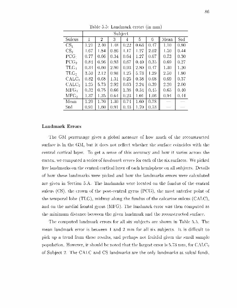
86

Table 5.5: Landmark errors (in mm)

Subject

Sulcus 1 2 3 4 5 6 Mean Std

CS1 1.21 2.40 1.48 0.22 0.63 0.47 1.10 0.80

CS2 1.67 1.84 0.86 1.17 1.27 2.02 1.50 0.44

PCG1 0.77 0.66 0.34 0.64 1.27 0.67 0.73 0.30

PCG2 0.84 0.96 0.93 0.67 0.40 0.35 0.69 0.27

TLG1 0.34 0.60 2.90 0.93 2.80 0.47 1.30 1.20

TLG2 3.50 2.12 0.98 1.25 5.73 1.29 2.50 1.80

CALC1 0.82 0.68 1.31 0.25 0.38 0.68 0.69 0.37CALC2 1.25 5.73 2.92 0.63 2.24 0.39 2.20 2.00

MFG1 0.32 0.75 0.66 1.38 0.34 0.45 0.65 0.40

MFG2 1.37 1.35 0.64 0.23 1.01 1.06 0.94 0.44

Mean 1.20 1.70 1.30 0.74 1.60 0.78 { {

Std 0.91 1.60 0.91 0.43 1.70 0.53 { {

Landmark Errors

The GM percentage gives a global measure of how much of the reconstructed

surface is in the GM, but it does not re ect whether the surface coincides with the

central cortical layer. To get a sense of this accuracy and how it varies across the

cortex, we computed a series of landmark errors for each of the six surfaces. We picked

�ve landmarks on the central cortical layer of each hemisphere on all subjects. Details

of how these landmarks were picked and how the landmarks errors were calculated

are given in Section 5.A. The landmarks were located on the fundus of the central

sulcus (CS), the crown of the post-central gyrus (PCG), the most anterior point of

the temporal lobe (TLG), midway along the fundus of the calcarine sulcus (CALC),

and on the medial frontal gyrus (MFG). The landmark error was then computed as

the minimum distance between the given landmark and the reconstructed surface.

The computed landmark errors for all six subjects are shown in Table 5.5. The

mean landmark error is between 1 and 2 mm for all six subjects. It is diÆcult to

pick up a trend from these results, and perhaps not fruitful given the small sample

population. However, it should be noted that the largest error is 5.73 mm, for CALC2

of Subject 2. The CALC and CS landmarks are the only landmarks at sulcal fundi,

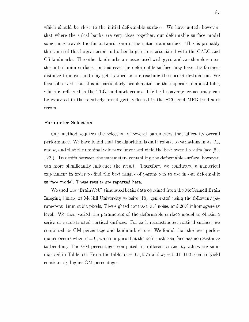
87

which should be close to the initial deformable surface. We have noted, however,

that where the sulcal banks are very close together, our deformable surface model

sometimes travels too far outward toward the outer brain surface. This is probably

the cause of this largest error and other large errors associated with the CALC and

CS landmarks. The other landmarks are associated with gyri, and are therefore near

the outer brain surface. In this case the deformable surface may have the farthest

distance to move, and may get trapped before reaching the correct destination. We

have observed that this is particularly problematic for the superior temporal lobe,

which is re ected in the TLG landmark errors. The best convergence accuracy can

be expected in the relatively broad gyri, re ected in the PCG and MFG landmark

errors.

Parameter Selection

Our method requires the selection of several parameters that a�ect its overall

performance. We have found that the algorithm is quite robust to variations in �1, �2,

and �, and that the nominal values we have used yield the best overall results (see [84,

122]). Tradeo�s between the parameters controlling the deformable surface, however,

can more signi�cantly in uence the result. Therefore, we conducted a numerical

experiment in order to �nd the best ranges of parameters to use in our deformable

surface model. These results are reported here.

We used the \BrainWeb" simulated brain data obtained from the McConnell Brain

Imaging Centre at McGill University website [18], generated using the following pa-

rameters: 1mm cubic pixels, T1-weighted contrast, 3% noise, and 20% inhomogeneity

level. We then varied the parameters of the deformable surface model to obtain a

series of reconstructed cortical surfaces. For each reconstructed cortical surface, we

computed its GM percentage and landmark errors. We found that the best perfor-

mance occurs when � = 0, which implies that the deformable surface has no resistance

to bending. The GM percentages computed for di�erent � and k2 values are sum-

marized in Table 5.6. From the table, � = 0:5; 0:75 and k2 = 0:01; 0:02 seem to yield

consistently higher GM percentages.

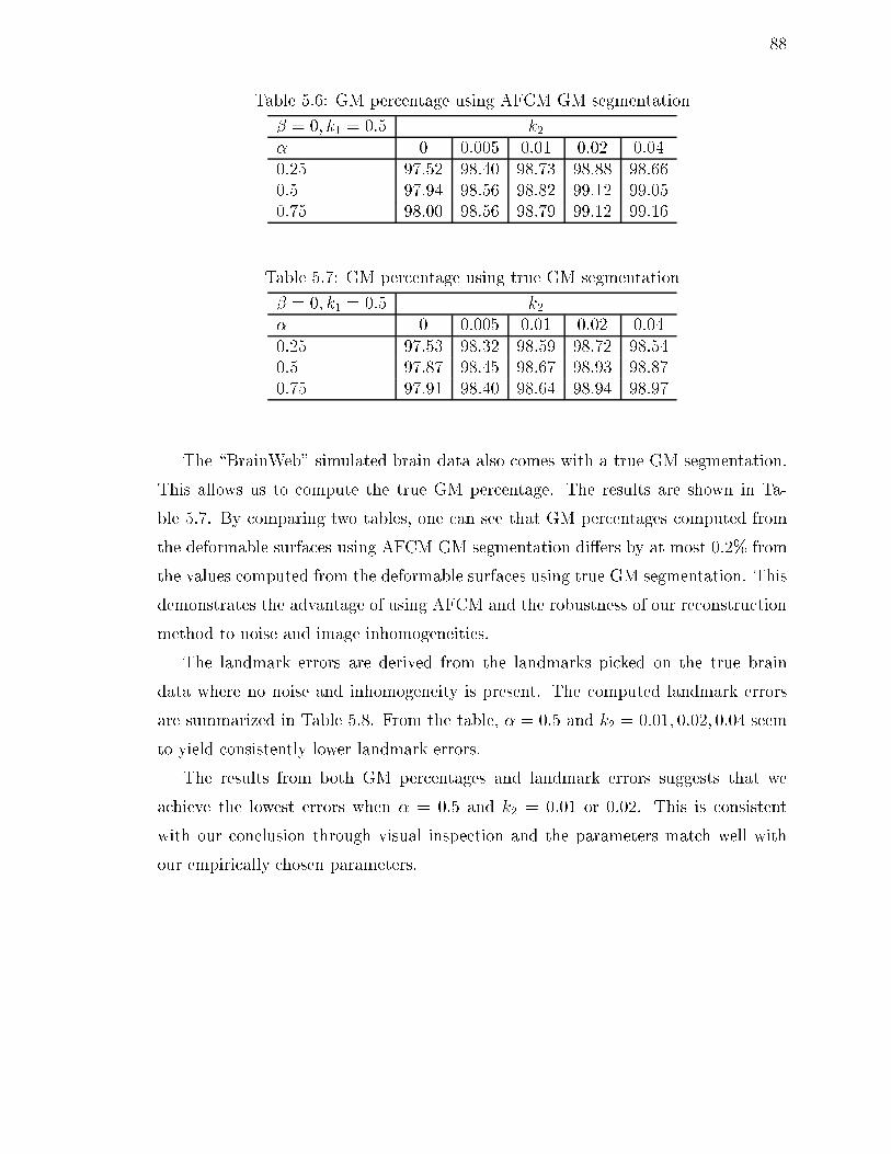
88

Table 5.6: GM percentage using AFCM GM segmentation

� = 0; k1 = 0:5 k2� 0 0.005 0.01 0.02 0.04

0.25 97.52 98.40 98.73 98.88 98.66

0.5 97.94 98.56 98.82 99.12 99.05

0.75 98.00 98.56 98.79 99.12 99.16

Table 5.7: GM percentage using true GM segmentation

� = 0; k1 = 0:5 k2� 0 0.005 0.01 0.02 0.04

0.25 97.53 98.32 98.59 98.72 98.54

0.5 97.87 98.45 98.67 98.93 98.87

0.75 97.91 98.40 98.64 98.94 98.97

The \BrainWeb" simulated brain data also comes with a true GM segmentation.

This allows us to compute the true GM percentage. The results are shown in Ta-

ble 5.7. By comparing two tables, one can see that GM percentages computed from

the deformable surfaces using AFCM GM segmentation di�ers by at most 0.2% from

the values computed from the deformable surfaces using true GM segmentation. This

demonstrates the advantage of using AFCM and the robustness of our reconstruction

method to noise and image inhomogeneities.

The landmark errors are derived from the landmarks picked on the true brain

data where no noise and inhomogeneity is present. The computed landmark errors

are summarized in Table 5.8. From the table, � = 0:5 and k2 = 0:01; 0:02; 0:04 seem

to yield consistently lower landmark errors.

The results from both GM percentages and landmark errors suggests that we

achieve the lowest errors when � = 0:5 and k2 = 0:01 or 0:02. This is consistent

with our conclusion through visual inspection and the parameters match well with

our empirically chosen parameters.

89

(a) (b)

(c) (d)

Figure 5.13: Surface renderings of (a) shrink-wrapping method versus (b) proposedmethod. Cross-sections of (c) shrink-wrapping method versus (d) proposed method.

90

Table 5.8: Landmark errors for phantom data (in mm)

� = 0; k1 = 0:5 k2� 0 0.005 0.01 0.02 0.04

0.25 0.97 0.94 0.88 0.88 0.89

0.5 1.05 0.99 0.85 0.83 0.85

0.75 1.06 1.06 0.89 0.87 0.85

Comparison with Shrink-wrapping

\Shrink-wrapping" is a well-known approach to �nding a parametric representa-

tion of the brain surface [72, 94, 31, 95]. This approach uses a deformable surface

that is initialized as a simple geometric object (sphere or ellipsoid) outside the cortex,

and the surface is then pushed toward the cortex by the action of internal and exter-

nal forces. For comparative purposes, we implemented a shrink-wrapping deformable

model that started from an initial sphere outside the brain surface and deformed

toward the central layer of the GM using GGVF forces. The resulting surface of

Subject 1 is shown in Fig. 5.13a, while the surface found by our method is shown

in Fig. 5.13b. These surfaces look very similar, and it is not apparent from these

renderings that there is much di�erence in these approaches.

A profound di�erence between these two approaches is revealed, however, in the

cross-sectional images shown in Figs. 5.13c and 5.13d. Clearly, the shrink-wrapping

method only �nds the outermost cortical layer. It is interesting to note that the GM

percentage of the shrink-wrapping method is 94%, a fairly large number. However,

this number merely indicates that the �nal surface resides overwhelmingly within the

GM, but does not indicate how faithfully it tracks the entire cortex. In fact, the

landmark errors computed for the shrink-wrapping result shows substantial errors (4-

10 mm) in the CS, CALC, MFG landmarks, which are landmarks that either reside

within sulci or within the interhemispheric �ssure. This demonstrates the importance

of initializing the deformable surface from inside the cortical GM.

91

(a) (b) (c)

Figure 5.14: (a) Front and (b) lateral views of a cortical mean curvature map. (c)Colormap used for plotting the map.

5.3 Applications

5.3.1 Cortical Di�erential Geometry and Thickness Compu-

tation

Once the cortical surface has been extracted, di�erential geometry quantities may

be computed. Di�erential geometry provides a natural mathematical framework to

study the cortical surface geometry. Among many geometric quantities de�ned for the

surface, curvature information is the most valuable since it quanti�es the structure

of the sulci and gyri, thus providing the basis for scienti�c and comparative studies.

Our deformable surfaces are represented numerically using simplex meshes [37, 36]

as described in Appendix A.2.1. We have developed a robust algorithm to calculate

mean, Gaussian, and principal curvatures on a simplex mesh surface. Details about

the algorithm can be found in Appendix B.

Fig. 5.14 shows two views of the mean curvature, plotted on the extracted cortical

surface of our sample data set. In these �gures, black stands for positive mean

curvature values, gray stands for zero, and white stands for negative mean curvature

values. From the �gures, we see that sulci are described by black central \skeletons"

92

(a) (b) (c)

Figure 5.15: (a) Front and (b) lateral views of a cortical thickness map. (c) Colormapused for plotting the map.

surrounded by white regions. These skeletons, which are in the interior of the brain,

correspond to the \roots" of the sulci, while the white regions are the \lips" of the sulci

on the surface of the brain. This correspondence between the structure of sulci/gyri

and mean curvature provides the basis for brain geometry analysis.

We have recently implemented a preliminary algorithm to compute cortical thick-

ness in the vicinity of the central cortical layer estimate. For every point on the

surface, we search in the direction of the simplex mesh normal vector until the closest

peak in the gray matter membership function is located. If this peak is not above

0.7, then we are unable to calculate a legitimate thickness value. If this peak is above

0.7, then the thickness is calculated as the distance between the two points along the

unit normal at which the gray matter membership function falls below 0.2. A thick-

ness map resulting from this calculation is shown in Fig. 5.15, where black represents

5.0mm, gray represents 2.5mm, and white represents points at which the thickness

could not be reliably estimated. We note that this result is very preliminary, and

requires substantial improvements and validation, as is planned in the future work

summarized in Chapter 6.

93

5.3.2 A Spherical Map for Cortical Geometry

Characterizing normal versus abnormal cortical geometry is an important goal of

human brain mapping. This task proves diÆcult because of the convoluted nature of

the cortical surface. DiÆculties arise in both identifying topological landmarks and

obtaining reliable quantitative measurements. A standard measurement method is to

trace sulcal fundi or other regions of interest across 2-D slices in MRI scans. Accurate

measurements are diÆcult to obtain using this method because structures must be

identi�ed across slices and a true 3-D geometric analysis is not possible.

Here, we present a preliminary method for representing the cortical surface that

facilitates visualization and delineation of regions on the cortical surface. We generate

a spherical map for each cortical hemisphere so that the full extent of sulcal fundi

and the buried cortex within the sulcal folds can be visualized. The spherical map

has a one-to-one mapping with the reconstructed cortical surface. This allows regions

of interest to be identi�ed on the spherical map and accurate measurement analysis

to be made on the 3-D geometry of the cortical surface.

Six hemispheres from three MR brain images were analyzed. On each brain, the

topologically correct, central cortical layer was reconstructed. To create the spher-

ical map, the hemispheres were separated using a cut through the corpus callosum.

This caused an opening to be created around the cut path. Then, focusing on one

hemisphere, the opening was mapped to a circle. Next, an elastic relaxation process

was applied to the surface until it reached a convex shape. Then, a fast projection

method was used to transform the relaxed surface to a sphere. The mean curvature

of the cortex was plotted on the sphere using a gray-scale colormap. The resulting

spherical map of a typical hemisphere is shown in Fig. 5.16a. Large mean curvatures

appear dark so sulcal fundi are readily identi�ed as thin dark streaks. In Fig. 5.16a,

the region of cortex buried within the central sulcus (outlined in black) shows the

characteristic precentral knob of this sulcus. Fig. 5.16b shows this region of buried

cortex as it appears in the brain.

Using the techniques described, we have manually delineated the buried cortex

surrounding primary sulci on the spherical map. These regions are displayed on the

94

(a) (b)

Figure 5.16: (a) A spherical map depicting mean curvature. The central sulcus isoutlined in black. (b) Manually identi�ed central sulcus.

spherical map in Fig. 5.17a. These regions are also displayed on the reconstructed

cortical surface in Fig. 5.17b.

5.4 Summary

We presented a method for reconstructing cortical surfaces from MR brain images.

This method combines a fuzzy segmentation method, an isosurface algorithm, and

a new deformable surface model to reconstruct a surface representation of the corti-

cal central layer. The reconstructed surfaces include deep gyri and sulci and possess

the correct surface topology of the cortex. The process is mostly automated and pro-

duces surfaces that are typically within 1-2 mm of the correct location throughout the

cortex. We described some preliminary work on the application of cortical surface re-

construction. We developed a method for computing di�erential geometry quantities

on cortical surfaces and demonstrated the feasibility of calculating cortical thickness

map. Finally, we showed that spherical maps that have a one-to-one mapping with

reconstructed cortical surfaces can be constructed. This allows delineation of regions

of interest such as sulci on the spherical map and analysis of the segmented regions

on the convoluted surface.

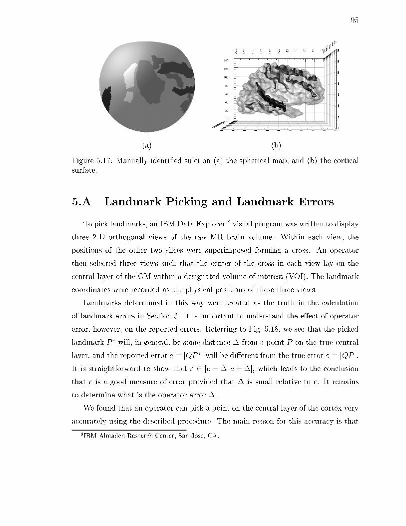
95

(a) (b)

Figure 5.17: Manually identi�ed sulci on (a) the spherical map, and (b) the corticalsurface.

5.A Landmark Picking and Landmark Errors

To pick landmarks, an IBM Data Explorer 8 visual program was written to display

three 2-D orthogonal views of the raw MR brain volume. Within each view, the

positions of the other two slices were superimposed forming a cross. An operator

then selected three views such that the center of the cross in each view lay on the

central layer of the GM within a designated volume of interest (VOI). The landmark

coordinates were recorded as the physical positions of these three views.

Landmarks determined in this way were treated as the truth in the calculation

of landmark errors in Section 3. It is important to understand the e�ect of operator

error, however, on the reported errors. Referring to Fig. 5.18, we see that the picked

landmark P � will, in general, be some distance � from a point P on the true central

layer, and the reported error e = jQP �j will be di�erent from the true error " = jQP j.It is straightforward to show that " 2 [e � �; e + �], which leads to the conclusion

that e is a good measure of error provided that � is small relative to e. It remains

to determine what is the operator error �.

We found that an operator can pick a point on the central layer of the cortex very

accurately using the described procedure. The main reason for this accuracy is that

8IBM Almaden Research Center, San Jose, CA.

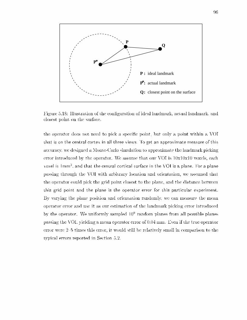
96

QP

ideal landmarkP

P actual landmark

Q closest point on the surface

:

:

:

*P

*

Figure 5.18: Illustration of the con�guration of ideal landmark, actual landmark, andclosest point on the surface.

the operator does not need to pick a speci�c point, but only a point within a VOI

that is on the central cortex in all three views. To get an approximate measure of this

accuracy, we designed a Monte-Carlo simulation to approximate the landmark picking

error introduced by the operator. We assume that our VOI is 10x10x10 voxels, each

voxel is 1mm3, and that the central cortical surface in the VOI is a plane. For a plane

passing through the VOI with arbitrary location and orientation, we assumed that

the operator could pick the grid point closest to the plane, and the distance between

this grid point and the plane is the operator error for this particular experiment.

By varying the plane position and orientation randomly, we can measure the mean

operator error and use it as our estimation of the landmark picking error introduced

by the operator. We uniformly sampled 109 random planes from all possible planes

passing the VOI, yielding a mean operator error of 0.04 mm. Even if the true operator

error were 2{5 times this error, it would still be relatively small in comparison to the

typical errors reported in Section 5.2.

97

Chapter 6

Conclusions and Future Work

This thesis considered the problem of mapping boundaries in digital images. We

developed two new deformable models and validated their performance both qualita-

tively and quantitatively on numerous examples. Based on the proposed deformable

models, we also developed a new method for cortical surface reconstruction and val-

idated this method using both simulated and real MR images. In this chapter we

summarize the main results and propose new directions for future research.

6.1 Gradient Vector Flow Deformable Models

In Chapter 3, we �rst generalized the force balance equations to allow use of

a general vector �eld rather than an irrotational (conservative) vector �eld. This

generalization led us to develop a general vector �eld called gradient vector ow

(GVF) computed through a vector di�usion process of the gradient of an edge map.

The GVF vector �eld can be used as an external force �eld for a deformable model

to reconstruct the parametric description of a target boundary.

The main results of this work and ideas for future work are summarized below.

98

6.1.1 Main Results

1. Both traditional external forces and distance potential forces are conservative

force �elds and do not point into boundary concavities, while GVF, which is a

general type of force �eld, does.

2. Unlike traditional external force �elds, the GVF �eld has a large capture range

without distorting the boundary.

3. Unlike balloon models, the GVF deformable model preserves perceptual bound-

aries.

4. Balloon models must be initialized completely inside or outside target bound-

aries because balloon forces can only push out or push in. The GVF deformable

model, however, can be initialized across boundaries as well.

5. Simulation results show that GVF can smooth out weak gradients while main-

taining strong gradients, which makes the deformable models using GVF per-

form robustly against image noise.

6.1.2 Future Work

Further investigations into the nature and uses of GVF are warranted. In partic-

ular, a complete characterization of the capture range of the GVF �eld would help

in deformable model initialization procedures. It would also help to more fully un-

derstand the GVF parameter �, perhaps �nding a way to choose it optimally for a

particular image, and to understand the interplay between � and the internal force

weighting parameters � and �. Finally, the GVF framework might be useful in de�n-

ing new connections between parametric and geometric deformable models, and might

form the basis for a new geometric rather than parametric deformable model.

99

6.2 Generalized Gradient Vector Flow Deformable

Models

In Chapter 4, we developed a generalization of the GVF formulation called general-

ized gradient vector ow (GGVF, which incorporates two spatially-varying weighting

functions. This new formulation can produce a numerically faster di�usion process in

homogeneous regions while maintaining excellent boundary localization capabilities.

We also noted that GGVF can be used as new way to represent images by encoding

both boundary information and medialness information in one representation. Fi-

nally, we exploited the medialness property of the GGVF and developed a method to

reconstruct the central layer of thick boundaries.

6.2.1 Main Results

1. Simulation results show that GGVF improves deformable model convergence

into long, thin boundary indentations, and maintains other desirable properties

of GVF, such as an extended capture range.

2. On a series of simulated images, we compared the boundary localizing accu-

racy of deformable models using GGVF, GVF, distance potential forces, and

traditional external forces, which are initialized at the true location of target

boundaries to study the ideal best performance of each model. Our results show

that deformable models using GGVF, GVF, distance potential forces, and tradi-

tional external forces (� = 1) all yield high accuracy consistently with maximum

radial errors less than 0.75 pixels, while the performance of deformable models

using external forces with larger smoothing parameter (� = 3 and � = 6) de-

generates almost linearly with respect to the increase of boundary undulation.

This indicates that traditional forces with larger smoothing parameter is not

suitable for reconstructing objects with convoluted boundaries even though the

deformable model starts at the desired boundary.

3. Simulation results show that the performance of both the GGVF deformable

100

model (MRE = 2.2) and the GVF deformable model (MRE = 2.3) is not sen-

sitive to impulsive noise present in the images while the performance of other

methods degenerated signi�cantly.

4. Simulation results show that GGVF deformable models can accurately recon-

struct the central layer of boundaries with thickness less than 6 pixels wide

with MREs less than 0.7 pixels, while the reconstruction is less accurate with

MREs almost doubled when the boundary thickness is 9 pixels wide. This re-

sult demonstrates the applicability of GGVF deformable models in the human

brain cortex reconstruction since the cortex usually has thickness between 3 to

5 voxels.

6.2.2 Future Work

In future research, we would like to study other choices of weighting functions and

their implications in the behavior of deformable models. Also, further investigation of

the GGVF medialness properties and possible �nding of its mathematical relationship

to classical medialness such as skeleton and cores may shed new light on the research

of shape representation. The current formulation of GGVF is in Euclidean spaces.

It would be interesting to investigate the possibility of extending its formulation

onto manifolds, especially surfaces. Finally, making connections between GGVF with

other applications in image processing and computer vision might provide some new

insights or even new solutions to existing problems.

6.3 Brain Cortex Reconstruction

In Chapter 5, we developed a method for reconstructing cortical surfaces from

MR brain images. This new method is largely automated. The method uses a novel

approach to initialize deformable models using isosurface algorithms. It reconstructs

the cortical surfaces including deep gyri and sulci and possessing the correct surface

topology. We developed two performance measures: gray matter percentage and

landmark error, which allows us to quantify the performance of our methods on real

101

brain MR images. We developed a method to compute di�erential geometry quantities

for the cortical surface reconstructed. We carried out a preliminary investigation on

generating a spherical map from reconstructed cortical surface.

6.3.1 Main Results

1. Experimental results show that the topology of isosurfaces can be corrected by

median �ltering the WM membership function iteratively.

2. Experimental results show that reliable and robust cortical surface reconstruc-

tion results can be achieved by applying deformable models on the fuzzy mem-

bership functions instead of on the raw intensity images.

3. Experimental results show that for six volumetric brain MR images with voxels

size on the order of 1mm3, our reconstruction method can produce surfaces that

are typically within 1-2 mm of the correct location throughout the cortex.

4. Experimental results show that the gray matter percentages of the reconstructed

cortical surfaces are consistently above 96.5%.

5. The proposed method produces signi�cantly better results than does a con-

ventional shrink-wrapping method. In an experiment, the proposed method

produced a gray matter percentage of 98% and landmark errors between 0.32

mm and 3.50 mm (with an average of 1.2 mm) whereas the shrink-wrapping

method yielded a gray matter percentage of 94% and substantial landmark er-

rors between 4 mm and 10 mm.

6.3.2 Future Work

Future work includes reduction of the required manual intervention and improved

convergence to narrow, extended gyri. Since the initial surface is already very dense,

we cannot use usual subdivision technique to decrease the running time of the model.

However, implementing the deformable models in a multiresolution fashion can sig-

ni�cantly reduce the running time. Due to imaging resolution, the intensities of

102

certain GM/GM interface in the sulci may appear to be completely at in the GM

membership function, which can lead to a location shift in the reconstructed central

cortical surface in these regions. We would like to incorporate anatomical constraints

to address this problem. Accurate thickness estimation is an important area of future

research. We believe that improved results will be obtained by incorporating more

prior knowledge about thickness variability. Our current approach to spherical map-

ping is time consuming (usually 12 hours), and generates a spherical map without

using any distortion minimization criteria. Further research in this area is expected

to focus on reducing running time and minimizing length, angle, or area distortion.

Furthermore, since our work on cortical surface reconstruction generates a map-

ping of entire cortical surface, study of various brain structures can now be done in a

more precise way. Also functional data can be mapped onto the reconstructed corti-

cal surface to study the relationship between structure and function hence to further

enhance our understand about the brain.

6.4 Overall Perspective

The main goal of the work presented in this thesis has been to contribute to

boundary mapping through the development of new deformable models, and to in-

vestigate their application to brain cortex reconstruction from MR images. It is

hoped that the research herein can deepen the understanding of deformable models

and point out new directions for designing better deformable models and extending

their applications into other areas in medical imaging, image analysis and computer

vision.

103

Appendix A

Deformable Model Implementation

In this appendix, the implementation of both deformable contours and surfaces is

described.

A.1 Deformable Contours

Both the traditional deformable contour model and the GGVF(GVF) deformable

contour model can be characterized by the following dynamic equation

8<:xt(s; t) = (�(s)x0(s; t))0 � (�(s)x00(s; t))00 + Fext(x)

x(s; 0) = x0(s)(A.1)

where Fext is the external force and x0 denotes the partial derivative of x with respect

to s. The equation reduces to Eq. (3.2) when the values of � and � are chosen to be

constants.

Approximating the derivatives with �nite di�erences, and converting to the vector

notation xi = (xi; yi) = (x(ih); y(ih)), we can rewrite Eq. (A.1) as

xit � xi

t�1

�= ��i(x

t

i� xt

i�1) + �i+1(xt

i+1 � xti)

��i�1(xti�2 � 2xti�1 + xt

i)

+2�i(xt

i�1 � 2xti+ xt

i+1)

��i+1(xti � 2xti+1 + xt

i+2) + Fext(xt�1i

) (A.2)

104

where xi = x(ih), �i = �(ih), �i = �(ih), h the step size in space, and � the step size

in time. In general, the external force Fext is stored as a discrete vector �eld, i.e., a

�nite set of vectors de�ned on an image grid. The value of Fext at any location xi

can be obtained through a bilinear interpolation of the external force values at the

grid points near xi.

Eq. (A.2) can be written in a compact matrix form as

xt � xt�1

�= Axt + Fext(x

t�1) (A.3)

where A is a pentadiagonal banded matrix.

Eq. (A.3) can then be solved iteratively by matrix inversion:

xt = (I� �A)�1(xt�1 + �Fext(xt�1)): (A.4)

We note that since the above �nite di�erence scheme is implicit with respect to the

internal forces, it can solve very rigid deformable contours with large step sizes [62, 4].

A.2 Deformable Surfaces

A typical dynamic deformable surface model is described in Eq. (2.10). It can be

expanded and written as the following:

8<:xt(u; t) = �r2

ux(u; t)� �r2

u(r2

ux(u; t)) + Fext(x)

x(u; 0) = x0(u):(A.5)

In order to �nd a solution to this dynamic partial di�erential equation, it is necessary

to represent the continuous deformable surface x with a discrete mesh. It is possible to

use either �nite-element methods (cf. [19, 21, 76]) or Fourier basis methods (cf. [100,

101]) to solve Eq. (A.5). These methods, however, are slow for meshes with a large

number of nodes. On the other hand, �nite di�erence methods (cf. [36, 42, 27])

based on polygon mesh models requires only simple arithmetic operations at each

node of the mesh and therefore are more suitable for implementing meshes with a

large number of nodes, such as those used in cortical surface reconstruction. In our

105

work, we implemented the deformable surfaces using the �nite di�erence method on

a polygon mesh model called the simplex mesh [37, 36, 38].

In this section, we �rst introduce the de�nition of simplex meshes. We then

describe how to generate simplex meshes. Finally, we describe how to implement

deformable surfaces represented by the simplex mesh. We note that all surfaces and

their corresponding meshes described in the rest of the appendix are assumed to be

closed although we expect our discussions are applicable to open surfaces with minor

modi�cation.

A.2.1 Simplex Meshes: a Surface Representation for De-

formable Surfaces

A simplex mesh is a polygon mesh where each node or vertex on the mesh has

a constant number of connections to its neighbors. A simplex mesh can be de�ned

in any dimension. A k-simplex mesh is de�ned as a (k + 1)-connected mesh where

each vertex has exactly (k + 1) neighbors. Formally, a k�Simplex Mesh M of Rd is

de�ned as a pair (V (M); N(M)) where V (M) is the set of vertices of M given by

V (M) = fPig; i 2 f1; : : : ; ng; Pi 2 Rd (A.6)

and N(M) is the associated connectivity function de�ned by

N(M) : f1; : : : ; ng �! f1; : : : ; ngk+1

such that

8i 2 f1; : : : ; ng; i 7�! (N1(i); N2(i); : : : ; Nk+1(i)) (A.7)

and

8i 2 f1; : : : ; ng; 8j 2 f1; : : : ; k + 1g; 8l 2 f1; : : : ; k + 1g; l 6= j

(1) Nj(i) 6= i (A.8)

(2) Nl(i) 6= Nj(i); (A.9)

Conditions Eq. (A.8) and (A.9) prevent a mesh from exhibiting loops or double edges

as shown in Fig. A.1. We further restrict a k-simplex mesh to be connected in such a

106

(a) (b)

Figure A.1: (a) a loop; (b) double edges.

Figure A.2: A simplex mesh.

way that for any two vertices there exists a path joining them. In our work, we will

only consider 2-simplex meshes in R3.

From the de�nition of a k-simplex mesh, we know that a 2-simplex mesh must

be a 3-connected mesh. This is an important property that is used to simplify and

speed up the deformable surface implementation in Section A.2.4. An example of a

2-simplex mesh is shown in Fig. A.2. A 2-simplex mesh can represent any type of

3-D surface and will be simply referred from now on as a simplex mesh.

Another type of polygon mesh representation used frequently in computer graphics

is a mesh consisting of only triangles (triangle meshes). Triangle meshes in general are

107

Dual Operation

Face

Edge

Vertex

a segment of triangle mesh the dual mesh

Figure A.3: Illustration of a dual operation.

easier to construct. They have been studied extensively for many years and techniques

for constructing them are readily available (cf. [44, 97]). It can be shown that triangle

meshes can be used to generate simplex meshes through a dual operation [37]. By

de�nition, a dual operation on a polygon mesh constructs a new mesh where each

vertex in the new mesh corresponds to a face in the original mesh and each face in

the new mesh corresponds to a vertex in the original mesh as shown in Fig. A.3.

The duality between triangle meshes and simplex meshes gives rise to a convenient

way to construct simplex meshes by computing the dual mesh of the triangle meshes.

In next two sections, we �rst review two triangle mesh generation methods used

frequently in computer graphics. We then describe in details about how to implement

the dual operation.

A.2.2 Triangle Mesh Generation

Here we describe two well-known methods for generating triangle meshes. The

�rst method starts with a sparse triangle mesh and subdivides each triangle into four

smaller triangles recursively to generate a denser triangle mesh. The second method

starts from an image volume and computes isosurfaces to generate triangle meshes.

108

subdivision

Figure A.4: A triangle and its subdivided triangles.

Subdivision method

A subdivision operation on a single triangle is shown in Fig. A.4. When a subdivi-

sion is applied on a triangle mesh, each triangle is replaced by four smaller triangles.

This operation can be repeated recursively to achieve arbitrary resolution.

Subdivision can be tailored and used in a variety of applications [40, 55, 126]. One

application of subdivision is to generate a triangle mesh that approximates a sphere as

accurately as possible. This mesh can then be used to initialize a deformable surface.

To create such a mesh, one can start by constructing an icosahedron directly, and then

subdivide and project the subdivided vertices onto a sphere recursively to generate a

more accurate approximation of a sphere [82]. Fig. A.5 illustrates this process. Note

that the three objects shown in Fig. A.5 use 20, 80, and 320 approximating triangles,

respectively.

Isosurface method

An isosurface is a surface that passes through all locations in space where a

continuous data volume is equal to a constant value, called the isosurface threshold.

The result of most isosurface algorithms is a surface tessellated, in particular, into a

triangle mesh. The construction of an isosurface is a well-studied problem [71, 79].

The marching cubes algorithm proposed by Lorensen and Cline [71] has received a

great amount of attention in recent years. It and its variants have become the standard

for generating isosurfaces and are used in many commercial visualization software

109

(a) (b) (c)

Figure A.5: Subdividing to improve a triangular approximation to a sphere.

packages. Below, we give a concise description of the marching cubes algorithm.

Marching cubes works directly with the volume data by breaking the volume into

voxels. Each voxel is a cube with 8 vertices. Depending on whether the intensity

value at a cube vertex is bigger or smaller than the isosurface threshold, a boolean

value of 1 or 0 is assigned to that vertex. It can then be shown that there are 256

total possible ways a surface can pass through the cube. If one takes into account

complementary and rotational symmetry, this number reduces to 14 unique con�g-

urations. From those con�gurations, one or more triangles are constructed for that

cube using interpolation. This process is repeated throughout the volume by linear

scanning.

Although marching cubes is an e�ective algorithm, it has been shown that it

can create surface holes in certain cases. Kalvin et al. [60] proposed a variation of

marching cubes called Alligator which solves the ambiguity problem by constraining

the triangle partition of each cube using connectivity information. In Fig. A.6, we

show a brain triangle mesh obtained by computing an isosurface from a 3-D MR brain

image using the Alligator algorithm.

110

Figure A.6: Surface rendering of a brain triangle mesh obtained by computing the

isosurface from a brain image volume and its zoom view with edges superimposed onthe mesh.

A.2.3 Simplex Mesh Generation through Dual Operation on

Triangle Meshes

The de�nition of a dual operation introduced in Section A.2.1 is straightforward.

Its implementation, however, is not trivial. If the polygon mesh is not in a suitable

representation, the dual operation can be diÆcult to implement and time consuming.

Moreover, the mesh representation must be general enough to describe both triangle

meshes and simplex meshes. A particular mesh representation in computer graphics

called winged-edge representation has been developed to address these problems [7].

In this section, we give a brief description of winged-edge representation in the context

of our work. We also outline the algorithm for implementing the dual operation based

on winged-edge representation. Finally, we show several results obtained using the

implemented dual operation.

Let us denote a mesh M = fV;E; Fg where V is the set of vertices, E is the set

of edges, and F is the set of faces. We also denote the number of vertices, the number

of edges, and the number of faces as KV , KE, and KF respectively. A winged-edge

111

representation of a mesh M can be described by the following collection of lists

Vertex list: fVig = f(xi; yi; zi)g; i = 1; 2; : : : ; KV

Edge list: fEig = f(vi1 ; vi2)g; i = 1; 2; : : : ; KE

Face list: fFig = f(ni; ei1 ; ei2; : : : ; eini )g; i = 1; 2; : : : ; KF

Edge neighbor list: N(Ei) = f(fi1 ; fi2)g; i = 1; 2; : : : ; KE

Vertex neighbor list: N(Vi) = f(mi; ei1 ; ei2 ; : : : ; eimi)g; i = 1; 2; : : : ; KV :

where Vi, Ei, and Fi are the ith vertex, edge, and face respectively. (xi; yi; zi) is the

coordinate of Vi. vi, ei, and fi are the indices of Vi, Ei, and Fi in their respective lists.

N(Ei) lists a pair of neighboring faces to an edge. N(Vi) lists a set of neighboring

vertices to a vertex, and ni and mi are the number of elements in Fi and N(Vi).

Finally, a counter clockwise order with respect to the outward unit face (vertex)

normal is imposed to the face (vertex neighbor) list.

Winged-edge representation allows fast implementation of various mesh opera-

tions. Here we de�ne a set of operations that are necessary to implement the dual

mesh.

Given an arbitrary index i, query operators for the ith vertex, edge, or face can

be de�ned as

V (i) = Vi

E(i) = Ei

F (i) = Fi:

The operator that computes the next index to i in a n-element list is de�ned as

next(i; n) = mod(i; n) + 1

where mod(i; n) is the modulus function. The operator that queries the jth vertex

on the face Fi is de�ned as

Vj(Fi) = V (Eij\ Einext(j;ni)

) = V (E(eij) \ E(einext(j;ni))):

112

(a) (b) (c)

Figure A.7: The dual meshes of meshes shown in Fig. A.5.

The operator that computes the center of a face Fi is de�ned as

center(Fi) =1

ni

niXj=1

Vj(Fi):

Using these operators de�ned, we can compute the dual mesh M = fV ; E; Fg ofthe mesh M using the following steps:

1. Vertex: Vi = center(Fi)

2. Edge: Ei = N(Ei)

3. Face: Fi = N(Vi)

4. Edge neighbor: N(Ei) = Ei

5. Vertex neighbor: N(Vi) = Fi

The results of applying the dual operation on the meshes shown in Fig. A.5 and

Fig. A.6 are shown in Fig. A.7 and Fig. A.8, respectively.

A.2.4 Deformable Surface Implementation

By discretizing the dynamic equation Eq. (A.5) on the simplex mesh using the

�nite di�erence method [53], we have the following di�erence equation for an arbitrary

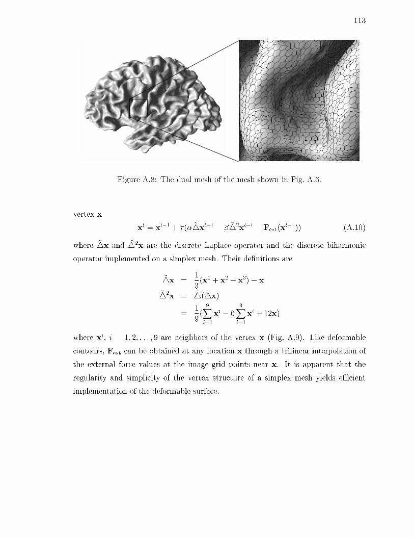
113

Figure A.8: The dual mesh of the mesh shown in Fig. A.6.

vertex x

xt = xt�1 + �(� ~4xt�1 � � ~42xt�1 + Fext(xt�1)) (A.10)

where ~4x and ~42x are the discrete Laplace operator and the discrete biharmonic

operator implemented on a simplex mesh. Their de�nitions are

~4x =1

3(x1 + x2 + x3)� x

~42x = ~4( ~4x)

=1

9(

9Xi=4

xi � 63X

i=1

xi + 12x)

where xi, i = 1; 2; : : : ; 9 are neighbors of the vertex x (Fig. A.9). Like deformable

contours, Fext can be obtained at any location x through a trilinear interpolation of

the external force values at the image grid points near x. It is apparent that the

regularity and simplicity of the vertex structure of a simplex mesh yields eÆcient

implementation of the deformable surface.

114

xx1

x4

x5

x6

x2

x7

x3

x8

x9

Figure A.9: Vertex structure on a simplex mesh.

115

Appendix B

Di�erential Geometry Quantities

on Simplex Meshes

In this appendix, we describe how the di�erential geometry quantities such as

Gaussian, mean, and principal curvatures can be computed from discrete surfaces

represented by simplex meshes. Since these di�erential geometry quantities require

derivatives up to the second order, the basic idea is to �t a paraboloid at each node

on a simplex mesh. After the coeÆcients of the paraboloid are estimated using a local

least square quadratic �t, all the di�erential geometry quantities can be computed on

the paraboloid through formulas found in di�erential geometry textbooks (cf. [39, 78]).

In order to �t a paraboloid at a given node on the simplex mesh, we need to

construct a local coordinate system at this node. To construct such a local coordinate

system, we �rst compute the unit normal, then translate the origin of the coordinate

system to the location of the given node, and rotate the coordinate system so that

the normal vector points upward in the new coordinate system. These steps are now

described in detail.

The unit normal at a given node P(0) on the simplex mesh can be approximated

using the following formula

N =P(1)�P(2) +P(2)�P(3) +P(3)�P(1)jjP(1)�P(2) +P(2)�P(3) +P(3)�P(1)jj (B.1)

where P(1);P(2);P(3) are P(0)'s three immediate neighbors and � is the vector cross

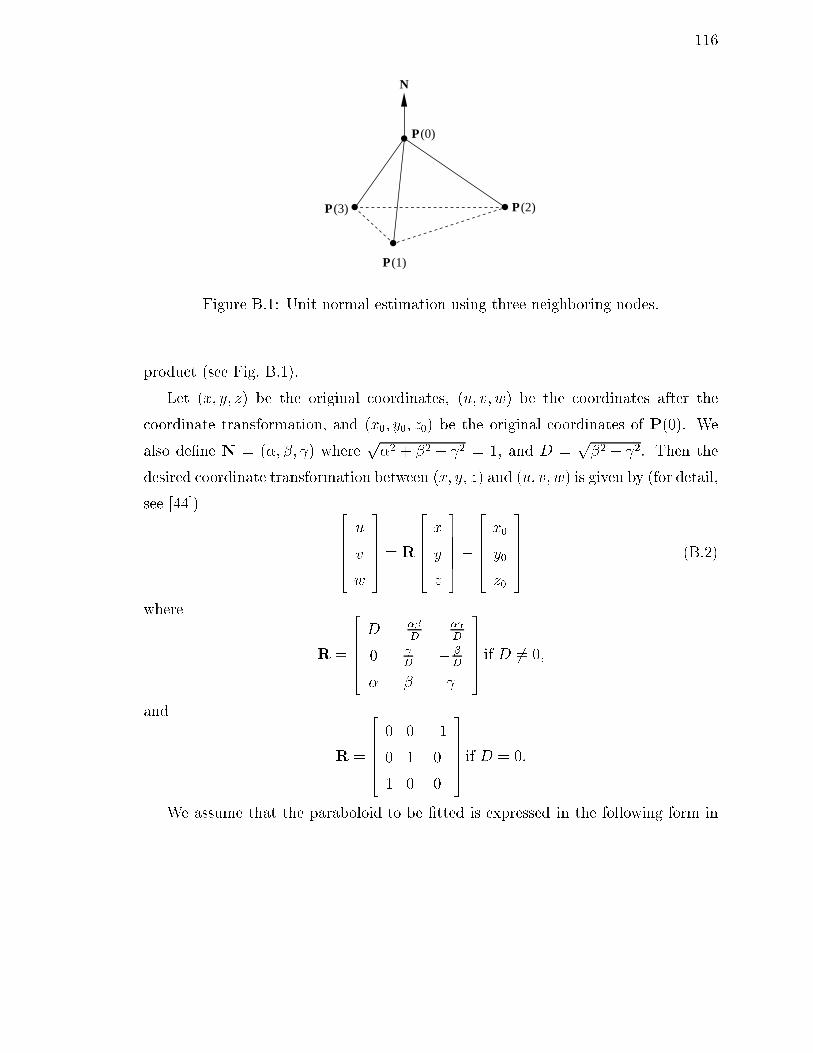
116

P(1)

P(3) P(2)

P(0)

N

Figure B.1: Unit normal estimation using three neighboring nodes.

product (see Fig. B.1).

Let (x; y; z) be the original coordinates, (u; v; w) be the coordinates after the

coordinate transformation, and (x0; y0; z0) be the original coordinates of P(0). We

also de�ne N = (�; �; ) wherep�2 + �2 + 2 = 1, and D =

p�2 + 2. Then the

desired coordinate transformation between (x; y; z) and (u; v; w) is given by (for detail,

see [44]) 266664u

v

w

377775 = R

266664x

y

z

377775�

266664x0

y0

z0

377775 (B.2)

where

R =

266664D ���

D��

D

0

D� �

D

� �

377775 if D 6= 0;

and

R =

2666640 0 �10 1 0

1 0 0

377775 if D = 0:

We assume that the paraboloid to be �tted is expressed in the following form in

117

the new coordinate system:

x(u; v) = (u; v; w) = (u; v; f(u; v)) = (u; v; h1u+ h2v +1

2h11u

2 + h12uv +1

2h22v

2)):

(B.3)

Let (ui; vi; f(ui; vi)); i = 1; 2; : : : ; q be the coordinates of P(0)'s neighbors and q be

the number of neighbors. The coordinates of the neighbors must satisfy the following

linear equations

266666664

u1 v112u21 u1v1

12v21

u2 v212u22 u2v2

12v22

......

......

...

uq vq12u2q

uqvq12v2q

377777775

266666666664

h1

h2

h11

h12

h22

377777777775=

266666664

w1

w2

...

wq

377777775

(B.4)

We now estimate [h1; h2; h11; h12; h22]T using singular value decomposition [89].

Now we are ready to compute di�erential geometry quantities derived from the

�tted paraboloid x(u; v) = (u; v; f(u; v)). The �rst and second derivatives of x are

computed as follows

xuj(0;0) = (1; 0; fu)j(0;0) = (1; 0; h1) (B.5)

xvj(0;0) = (0; 1; fv)j(0;0) = (0; 1; h2) (B.6)

xuuj(0;0) = (0; 0; fuu)j(0;0) = (0; 0; h11) (B.7)

xuvj(0;0) = (0; 0; fuv)j(0;0) = (0; 0; h12) (B.8)

xvuj(0;0) = (0; 0; fuu)j(0;0) = (0; 0; h12) (B.9)

xvvj(0;0) = (0; 0; fvv)j(0;0) = (0; 0; h22): (B.10)

The unit normal vector at x(0; 0) is given by

n =xu�xvjjxu�xvjj

j(0;0) = (�h1;�h2; 1)q1 + h1

2 + h22: (B.11)

The coeÆcients of the �rst fundamental form or the elements of metric tensor g at

x(0; 0) are given by [78]

g11 =< xu;xu > = 1 + h12 (B.12)

118

g12 =< xu;xv > = h1h2 (B.13)

g21 =< xv;xu > = h1h2 (B.14)

g22 =< xv;xv > = 1 + h22: (B.15)

The coeÆcients of second fundamental form are given by

L11 =< xuu;n > =h11q

1 + h12 + h2

2(B.16)

L12 =< xuv;n > =h12q

1 + h12 + h2

2(B.17)

L21 =< xvu;n > =h12q

1 + h12 + h2

2(B.18)

L22 =< xvv;n > =h22q

1 + h12 + h2

2(B.19)

Hence, the Weingarten map W is computed by

W = g�1L =

24 a

�

b

�

c

�

d

�

35 (B.20)

where g is the metric tensor, and

L =

24 L11 L12

L21 L22

35 (B.21)

� = det(g)32 = (1 + h1

2 + h22)

32 (B.22)

a = h11 + h11h22 � h12h1h2 (B.23)

b = h12 + h12h22 � h22h1h2 (B.24)

c = h12 + h12h12 � h11h1h2 (B.25)

d = h22 + h22h12 � h12h1h2: (B.26)

Therefore the characteristic polynomial of W is given by

�2 � a+ d

��+

ad� bc

�2= 0 (B.27)

The mean curvature H and Gaussian curvature K can now be computed as

H =a + d

2�=

(1 + h12)h22 + (1 + h2

2)h11 � 2h1h2h12

2(1 + h12 + h2

2)32

(B.28)

119

K =ad� bc

�2=

(h11h22 � h122)

(1 + h12 + h2

2)2: (B.29)

The principal curvatures are derived from mean curvature and Gaussian curvature as

k1 = H +pH2 �K (B.30)

k2 = H �pH2 �K (B.31)

where k1 and k2 are the maximum and minimum principal curvatures respectively.

At a nonumbilic point (where the principal curvatures are distinct), the corre-

sponding principal directions are given by

p1 =(b; a� k1�; 0)qb2 + (a� k1�)2

(B.32)

p2 =(b; a� k2�; 0)qb2 + (a� k2�)2

: (B.33)

120

Bibliography

[1] A. J. Abrantes and J. S. Marques, \A class of constrained clustering algorithms

for object boundary extraction," IEEE Trans. on Image Processing, vol. 5,

pp. 1507{1521, Nov. 1996.

[2] M. K. Agoston, Algebraic Topology | A �rst course. New York: Marcel Dekker,

Inc., 1976.

[3] L. Alvarez, F. Guichard, P. L. Lions, and J. M. Morel, \Axioms and fundamental

equations of image processing," Archive for Rational Mechanics and Analysis,

vol. 123, no. 3, pp. 199{257, 1993.

[4] W. F. Ames, Numerical Methods for Partial Di�erential Equations. Boston:

Academic Press, 3rd ed., 1992.

[5] A. A. Amini, T. E. Weymouth, and R. C. Jain, \Using dynamic programming

for solving variational problems in vision," IEEE Trans. on Pattern Anal. Ma-

chine Intell., vol. 12, no. 9, pp. 855{867, 1990.

[6] W. A. Barrett and E. N. Mortensen, \Interactive live-wire boundary extrac-

tion," Medical Image Analysis, vol. 1, no. 4, pp. 331{341, 1997.

[7] B. G. Baumgart, \A polyhedron representation for computer vision," Proc. of

the National Computer Conference, pp. 589{596, 1975.

[8] A. Blake and A. Zisserman, Visual Reconstruction. Boston: MIT Press, 1987.

[9] H. Blum and R. N. Nagel, \Shape description using weighted symmetric axis

features," Pattern Recognition, vol. 10, pp. 167{180, 1978.

121

[10] F. L. Bookstein, \Principal warps: Thin-plate splines and the decomposition of

deformations," IEEE Trans. on Pattern Anal. Machine Intell., vol. 11, no. 6,

pp. 567{585, 1989.

[11] V. Caselles, F. Catte, T. Coll, and F. Dibos, \A geometric model for active

contours," Numerische Mathematik, vol. 66, pp. 1{31, 1993.

[12] V. Caselles, R. Kimmel, and G. Sapiro, \Geodesic active contours," in Proc.

Fifth Int. Conf. on Comp. Vis., pp. 694{699, 1995.

[13] E. L. Chaney and S. M. Pizer, \De�ning anatomical structures from medical

images," Seminar in Radiation Oncology, vol. 2, pp. 215{225, Oct. 1992.

[14] A. H. Charles and T. A. Porsching, Numerical Analysis of Partial Di�erential

Equations. Englewood Cli�s, New Jersey: Prentice Hall, 1990.

[15] G. E. Christensen, S. C. Joshi, and M. I. Miller, \Volumetric transformation of

brain anatomy," IEEE Trans. Med. Imag., vol. 16, no. 6, pp. 864{877, 1997.

[16] G. E. Christensen, R. D. Rabbit, M. Miller, S. C. Joshi, U. Grenander,

T. Coogan, and D. V. Essen, \Topological properties of smooth anatomic

maps," in Information Processing in Medical Imaging, pp. 101{112, 1995.

[17] G. E. Christensen, R. D. Rabbitt, and M. I. Miller, \Deformable templates

using large deformation kinematics," IEEE Trans. on Image Processing, vol. 5,

pp. 1435{1447, Oct. 1996.

[18] C. A. Cocosco, V. Kollokian, R. K. S. Kwan, and A. C. Evans, \BrainWeb:

Online interface to a 3D MRI simulated brain database," Neuroimage, vol. 5,

no. 4, 1997. http://www.bic.mni.mcgill.ca/brainweb.

[19] I. Cohen, L. D. Cohen, and N. Ayache, \Using deformable surfaces to segment

3-D images and infer di�erential structures," CVGIP: Image Understanding,

vol. 56, pp. 242{263, Sept. 1992.

122

[20] L. D. Cohen, \On active contour models and balloons," CVGIP: Image Under-

standing, vol. 53, pp. 211{218, Mar. 1991.

[21] L. D. Cohen and I. Cohen, \Finite-element methods for active contour models

and balloons for 2-D and 3-D images," IEEE Trans. on Pattern Anal. Machine

Intell., vol. 15, pp. 1131{1147, Nov. 1993.

[22] D. Collins, C. Holmes, T. Peters, and A. Evans, \Automatic 3-D model-based

neuroanatomical segmentation," Human Brain Mapping, vol. 3, pp. 190{208,

1995.

[23] B. R. Condon, J. Patterson, et al., \Image non-uniformity in magnetic resonance

imaging: its magnitude and methods for its correction," The British Journal of

Radiology, vol. 60, pp. 83{87, 1989.

[24] T. F. Cootes, C. J. Taylor, D. H. Cooper, and J. Graham, \Active shape models

{ their training and application," Computer Vision and Image Understanding,

vol. 61, no. 1, pp. 38{59, 1995.

[25] R. Courant and D. Hilbert,Methods of Mathematical Physics, vol. 1. New York:

Interscience, 1953.

[26] R. Courant and D. Hilbert,Methods of Mathematical Physics, vol. 2. New York:

Interscience, 1989.

[27] A. M. Dale and M. I. Sereno, \Improved localization of cortical activity com-

bining EEG and MEG with MRI cortical surface reconstruction: A linear ap-

proach," J. Cogn. Neuroscience, vol. 5, no. 2, pp. 162{176, 1993.

[28] C. Davatzikos, Model-Based Boundary Mapping with Applications to Medical

Imaging. PhD thesis, The Johns Hopkins University, Baltimore, Maryland,

1994.

[29] C. Davatzikos, \Spatial normalization of 3D images using deformable models,"

Journal of Computer Assisted Tomography, vol. 20, no. 4, pp. 656{665, 1996.

123

[30] C. Davatzikos, \Spatial transformation and registration of brain images using

elastically deformable models," Computer Vision and Image Understanding,

vol. 66, pp. 207{222, May 1997.

[31] C. Davatzikos and R. N. Bryan, \Using a deformable surface model to obtain a

shape representation of the cortex," IEEE Trans. Med. Imag., vol. 15, pp. 785{

795, Dec. 1996.

[32] C. Davatzikos and J. L. Prince, \Convexity analysis of active contour models,"

in Proc. Conf. on Info. Sci. and Sys., pp. 581{587, 1994.

[33] C. Davatzikos and J. L. Prince, \An active contour model for mapping the

cortex," IEEE Trans. on Medical Imaging, vol. 14, pp. 65{80, Mar. 1995.

[34] L. Davis, Genetic Algorithms and Simulated Annealing. London: Pitman, 1987.

[35] B. M. Dawant, A. P. Zijidenbos, and R. A. Margolin, \Correction of intensity

variations in MR images for computer-aided tissue classi�cation," IEEE Trans.

Med. Imag., vol. 12, pp. 770{781, 1993.

[36] H. Delingette, \Adaptive and deformable models based on simplex meshes," in

Proceedings of the 1994 IEEE Workshop on Motion of Non-Rigid and Articu-

lated Objects, pp. 152{157, 1994.

[37] H. Delingette, \Simplex meshes: a general representation for 3D shape recon-

struction," Tech. Rep. TR2214, I.N.R.I.A., Sophia-Antipolis, France, Mar. 1994.

[38] H. Delingette, \Simplex meshes: a general representation for 3D shape recon-

struction," in Proc. IEEE Conf. Computer Vision and Pattern Recognition,

pp. 856{859, June 1994.

[39] M. P. do Carmo, Di�erential Geometry of Curves and Surfaces. Englewood

Cli�s, NJ: Prentice-Hall, 1976.

[40] D. Doo and M. Sabin, \Behaviour of recursive division surfaces near extraordi-

nary points," Computer-Aided Design, vol. 10, no. 6, pp. 356{360, 1978.

124

[41] H. A. Drury and D. C. V. Essen, \Functional specializations in human cere-

bral cortex analyzed using the visible man surface-based atlas," Human Brain

Mapping, vol. 5, pp. 233{237, 1997.

[42] H. A. Drury, D. C. V. Essen, C. H. Anderson, C. W. Lee, T. A. Coogan,

and J. W. Lewis, \Computerized mappings of the cerebral cortex: A multires-

olution attening method and a surface-based coordinate system," J. Cogn.

Neuroscience, pp. 1{28, 1996.

[43] M. A. Fischler and R. A. Elschlager, \The representation and matching of

pictorial structures," IEEE Trans. on Computers, vol. 22, no. 1, pp. 67{92,

1973.

[44] J. D. Foley, A. van Dam, S. K. Feiner, and J. F. Hughes, Computer Graphics:

Principles and Practice. Reading, MA: Addison-Wesley, 2nd ed. ed., 1990.

[45] S. Geman and D. Geman, \Stochastic relaxation, Gibbs distrutions, and the

Bayesian restoration of images," IEEE Trans. on Pattern Anal. Machine Intell.,

vol. 6, pp. 721{741, 1984.

[46] A. F. Goldszal, C. Davatzikos, D. L. Pham, M. X. H. Yan, R. N. Bryan, and

S. M. Resnick, \An image processing system for qualitative and quantitative

volumetric analysis of brain images," Journal of Computer Assisted Tomogra-

phy, to appear.

[47] R. C. Gonzalez and R. E. Woods, Digital Image Processing. Reading, MA:

Addison-Wesley, 1993.

[48] L. D. GriÆn, \The intrinsic geometry of the cerebral cortex," Journal of The-

oretical Biology, vol. 166, no. 3, pp. 261{273, 1994.

[49] W. E. L. Grimson, Ojbect Recognition by Computer: The Role of Geometric

Constraints. Cambridge, MA: MIT Press, 1990.

125

[50] W. E. L. Grimson, G. J. Ettinger, T. Kapur, M. E. Leventon, W. M. W. III,

and R. Kikinis, \Utilizing segmented mri data in image-guided surgery," Int.

J. Pattern Recog. Artif. Intell., vol. 11, no. 8, pp. 1367{1397, 1996.

[51] S. N. Gupta and J. L. Prince, \Stochastic models for DIV-CURL optical ow

methods," IEEE Signal Processing Letters, vol. 3, no. 2, pp. 32{35, 1996.

[52] K. E. Gustafson, Partial Di�erential Equations. New York: John Wiley & Sons,

2 ed., 1987.

[53] B. Heinrich, Finite Di�erence Methods on Irregular Networks. A Generalized

Approach to Second Order Elliptic Problems. Basel, Switzerland: Birkh�auser

Verlag, 1987.

[54] F. B. Hilderbrand, Methods of Applied Mathematics. Englewood Cli�s, NJ:

Prentice-Hall, 2 ed., 1965.

[55] H. Hoppe, Surface Reconstruction from Unorganized Points. PhD thesis, De-

partment of Computer Science and Engineering, University of Washington, June

1994.

[56] B. K. P. Horn, Robot Vision. Cambridge, MA: MIT Press, 1986.

[57] B. K. P. Horn and B. G. Schunck, \Determining optical ow," Arti�cial Intel-

ligence, vol. 17, pp. 185{203, 1981.

[58] A. K. Jain, Fundamentals of Digital Image Processing. Englewood Cli�s, NJ:

Prentice-Hall, 1989.

[59] S. Joshi, J. Wang, M. I. Miller, D. C. V. Essen, and U. Grenander, \On the

di�erential geometry of the cortical surface," in Proc. of the SPIE: Vision Ge-

ometry IV, vol. 2573, pp. 304{311, Aug. 1995.

[60] A. D. Kalvin, C. B. Cutting, B. Haddad, and M. Noz, \Constructing topolog-

ically connected surfaces for the comprehensive analysis of 3D medical struc-

126

tures," in SPIE Proc. Medical Imaging V: Image Processing, vol. 1445, pp. 247{

258, Feb. 1991.

[61] T. Kapur, E. Grimson, W. Wells, and R. Kikinis, \Segmentation of brain tis-

sue from magnetic resonance images," Medical Image Analysis, vol. 1, no. 2,

pp. 109{127, 1996.

[62] M. Kass, A. Witkin, and D. Terzopoulos, \Snakes: Active contour models,"

Int. J. Computer Vision, vol. 1, no. 4, pp. 321{331, 1987.

[63] B. B. Kimia, A. R. Tannenbaum, and S. W. Zucker, \Shapes, shocks, and

deformations I: The components of two-dimensional shape and the reaction-

di�usion space," Int. J. Computer Vision, pp. 189{224, 1995.

[64] R. Kimmel, A. Amir, and A. M. Bruckstein, \Finding shortest paths on surfaces

using level sets propagation," IEEE Trans. on Pattern Anal. Machine Intell.,

vol. 17, no. 6, pp. 635{640, 1995.

[65] G. J. Klein, P. T. S. X. Teng, and T. F. Budinger, \A sensitivity analysis

of brain morphometry based on MRI-derived surface models," in Proc. SPIE

Medical Imaging '98, vol. 3337, p. 31, 1998. abstract.

[66] A. C. W. Kotche� and C. J. Taylor, \Automatic construction of eigenshape

models by genetic algorithm," in the XVth Int. Conf. Inf. Proc. Med. Imag.

(IPMI), pp. 1{14, Springer-Verlag, 1997.

[67] F. Kruggel and G. Lohmann, \Automatical adaption of the stereotactical coor-

dinate system in brain MRI datasets," in the XVth Int. Conf. Inf. Proc. Med.

Imag. (IPMI), pp. 471{476, Springer-Verlag, 1997.

[68] B. Leroy, I. Herlin, and L. D. Cohen, \Multi-resolution algorithms for active

contour models," in 12th International Conference on Analysis and Optimiza-

tion of Systems, pp. 58{65, 1996.

127

[69] F. Leymarie and M. D. Levine, \Tracking deformable objects in the plane us-

ing an active contour model," IEEE Trans. on Pattern Anal. Machine Intell.,

vol. 15, no. 6, pp. 617{634, 1993.

[70] S. Lobregt and M. A. Viergever, \A discrete dynamic contour model," IEEE

Trans. on Medical Imaging, vol. 14, pp. 12{24, Mar. 1995.

[71] W. E. Lorensen and H. E. Cline, \Marching cubes: A high-resolution 3D surface

construction algorithm," ACM Comp. Graph., vol. 21, no. 4, pp. 163{170, 1987.

[72] D. MacDonald, D. Avis, and A. C. Evans, \Multiple surface identi�cation and

matching in magnetic resonance images," in SPIE Proc. VBC '94, vol. 2359,

pp. 160{169, 1994.

[73] R. Malladi, J. A. Sethian, and B. C. Vemuri, \Shape modeling with front prop-

agation: A level set approach," IEEE Trans. on Pattern Anal. Machine Intell.,

vol. 17, no. 2, pp. 158{175, 1995.

[74] J. F. Mangin, V. Frouin, I. Bloch, J. Regis, and J. Lopez-Krahe, \From 3D mag-

netic resonance images to structural representations of the cortex topography

using topology preserving deformations," Mathematical Imaging and Vision,

vol. 5, pp. 297{318, 1995.

[75] D. Marr, Vision. A computational investigation into the human representation

and processing of visual information. Freeman, 1982.

[76] T. McInerney and D. Terzopoulos, \A dynamic �nite element surface model for

segmentation and tracking in multidimensional medical images with application

to cardiac 4D image analysis," Computerized Medical Imaging and Graphics,

vol. 19, no. 1, pp. 69{83, 1995.

[77] T. McInerney and D. Terzopoulos, \Deformable models in medical image anal-

ysis: a survey," Medical Image Analysis, vol. 1, no. 2, pp. 91{108, 1996.

[78] R. S. Millman and G. D. Parker, Elements of Di�erential Geometry. Englewood

Cli�s, NJ: Prentice-Hall, 1977.

128

[79] C. Montani, R. Scateni, and R. Scopigno, \Discretized marching cubes," in

IEEE Proc. Visualization'94, pp. 281{287, 1994.

[80] P. M. Morse and H. Feshbach, Methods of Theoretical Physics. New York:

McGraw-Hill Book Company, 1953.

[81] D. Mumford and J. Shah, \Boundary detection by minimizing functionals," in

Proc. IEEE Conf. Computer Vision and Pattern Recognition, pp. 22{26, 1985.

[82] J. Neider, T. Davis, and M. Woo, OpengGL Programming Guide. Reading, MA:

Addison-Wesley, 1993.

[83] W. Neuenschwander, P. Fua, G. Szekely, and O. Kubler, \Making snakes con-

verge from minimal initialization," in ARPA Image Understanding Workshop,

pp. 1627{1636, 1994.

[84] D. L. Pham and J. L. Prince, \An adaptive fuzzy c-means algorithm for image

segmentation in the presence of intensity inhomogeneities," in SPIE Medical

Imaging '98: Image Processing, SPIE, Feb. 21-27, 1998.

[85] D. Pham and J. Prince, \An adaptive fuzzy c-means algorithm for image seg-

mentation in the presence of intensity inhomogeneities," to appear in Pattern

Recognition Letters, 1998.

[86] D. Pham and J. Prince, \Adaptive fuzzy segmentation of magnetic resonance

images," submitted to IEEE Trans. on Medical Imaging, 1998.

[87] S. M. Pizer, C. A. Burbeck, J. M. Coggins, D. S. Fritsch, and B. S. Morse,

\Object shape before boundary shape: Scale-space medial axes," Journal of

Mathematical Imaging and Vision, vol. 4, pp. 303{313, 1994.

[88] S. M. Pizer, W. R. Oliver, and S. H. Bloomberg, \Hierarchical shape description

via the multiresolution symmetric axis transform," IEEE Trans. on Pattern

Anal. Machine Intell., vol. 9, pp. 505{511, July 1987.

129

[89] W. H. Press, B. P. Flannery, S. A. Teukolsky, and W. T. Vetterling, Numerical

Recipes. Cambridge: Cambridge University Press, 1986.

[90] J. L. Prince and C. Xu, \A new external force model for snakes," in 1996 Image

and Multidimensional Signal Processing Workshop, pp. 30{31, 1996.

[91] J. Rademacher, A. M. Galaburda, D. N. Kennedy, P. A. Filipek, and

J. V. S. Caviness, \Human cerebral cortex: Localization, parcellation, and

morphometry with magnetic resonance imaging," Journal of Cognitive Neu-

roscience, vol. 4, pp. 352{374, 1992.

[92] J. Rauch, Partial Di�erential Equation. New York: Springer-Verlag, 1991.

[93] R. Ronfard, \Region-based strategies for active contour models," Int. J. Com-

puter Vision, vol. 13, no. 2, pp. 229{251, 1994.

[94] S. Sandor and R. Leahy, \Towards automated labelling of the cerebral cor-

tex using a deformable atlas," in Information Processing in Medical Imaging,

pp. 127{138, 1995.

[95] S. Sandor and R. Leahy, \Surface-based labeling of cortical anatomy using a

deformable atlas," IEEE Trans. Med. Imag., vol. 16, no. 1, pp. 41{54, 1997.

[96] G. Sapiro and A. Tannenbaum, \AÆne invariant scale-space," Int. J. Computer

Vision, vol. 11, no. 1, pp. 25{44, 1993.

[97] W. Schroeder, K. Martin, and B. Lorensen, The Visualization Toolkit. Engle-

wood Cli�s, NJ: Prentice-Hall, 2nd ed. ed., 1997.

[98] S. Sclaro� and A. Pentland, \On model modeling for medical images: Undercon-

strained shape description and data compression," in Proc. of IEEE Workshop

on Biomedical Image Analysis, pp. 70{79, 1994.

[99] N. W. Shock, R. C. Greulich, R. Andres, D. Arenberg, P. T. Costa Jr.,

E. Lakatta, and J. D. Tobin, \Normal human aging: The Baltimore longi-

130

tudinal study of aging." U.S. Governement Printing OÆce, Washington, D.C.,

1984.

[100] L. H. Staib and J. S. Duncan, \Boundary �nding with parametrically de-

formable models," IEEE Trans. on Pattern Anal. Machine Intell., vol. 14,

no. 11, pp. 1061{1075, 1992.

[101] L. H. Staib and J. S. Duncan, \Deformable Fourier models for surface �nding in

3D images," in Proc. Second Conf. on Visualization in Biomedical Computing,

vol. SPIE Proc., Vol. 1808, pp. 90{104, 1992.

[102] J. Talairach and P. Tournoux, Co-Planar Stereotaxic Atlas of the Human

Brain. 3-Dimensional Proportional System: An Approach to Cerebral Imaging.

Stuttgart, NY: Thieme Medical Publisher, Inc., 1988.

[103] H. Tek and B. B. Kimia, \Image segmentation by reaction-di�usion bubbles,"

in Proc. Fifth Int. Conf. on Comp. Vis., pp. 156{162, 1995.

[104] P. C. Teo, G. Sapiro, and B. A. Wandell, \Creating connected representations

of cortical gray matter for functional MRI visualization," IEEE Trans. Med.

Imag., vol. 16, no. 6, pp. 852{863, 1997.

[105] D. Terzopoulos, \On matching deformable models to images." Tech. Rept. 60.

Schlumberger Palo Alto research. 1986. Reprinted in Topical Meeting on Ma-

chine Vision, Technical Digest Series, Vol. 12, 1987, 160-167.

[106] D. Terzopoulos and K. Fleischer, \Deformable models," The Visual Computer,

vol. 4, pp. 306{331, 1988.

[107] D. Terzopoulos and R. Szeliski, \Tracking with Kalman snakes," in Active Vi-

sion (A. Blake and A. Yuille, eds.), Arti�cial Intelligence, pp. 3{20, Cambridge,

Massachusetts: The MIT Press, 1992.

[108] D. Terzopoulos, A. Witkin, and M. Kass, \Constraints on deformable models:

Recovering 3D shape and nonrigid motion," Arti�cial Intelligence, vol. 36, no. 1,

pp. 91{123, 1988.

131

[109] P. Thompson and A. W. Toga, \A surface-based technique for warping three-

dimensional images of the brain," IEEE Trans. on Medical Imaging, vol. 15,

pp. 402{417, Aug. 1996.

[110] M. Vaillant, C. Davatzikos, R. H. Taylor, and R. N. Bryan, \A path-

planning algorithm for image-guided neurosurgery," in Lecture Notes in Comp.

Sci.:CVRMed-MRCAS'97, vol. 1205, pp. 467{476, Mar. 1997.

[111] A. van Gelder and J. Wilhelms, \Topological considerations in isosurface gen-

eration," ACM Trans. on Graphics, vol. 13, pp. 337{375, 1994.

[112] D. von Seggern, Practical Handbook of Curve Design and Generation. CRC

Press, Inc., 1994.

[113] R. Whitaker, \Volumetric deformable models: Active blobs," Tech. Rep.

ECRC-94-25, European Computer-Industry Research Centre GmbH, 1994.

[114] B. Widrow, \The \rubber-mask" technique," Pattern Recognition, vol. 5,

pp. 175{211, 1973.

[115] C. Xu, M. E. Etemad, D. N. Yu, D. L. Pham, and J. L. Prince, \A spherical map

for cortical geometry." 4th International conference on Functional Mapping of

the Human Brain (HBM), June 7-12, 1998; NeuroImage 7(4):734, 1998.

[116] C. Xu, D. L. Pham, M. E. Etemad, D. N. Yu, and J. L. Prince, \Reconstruction

of the human cerebral cortex from magnetic resonance images." submitted to

IEEE Trans. on Medical Imaging on September 8, 1998.

[117] C. Xu, D. L. Pham, and J. L. Prince, \Reconstruction of the human cortical

surface from MR images." 4th International conference on Functional Mapping

of the Human Brain (HBM), June 7-12, 1998; NeuroImage 7(4):715, 1998.

[118] C. Xu, D. L. Pham, and J. L. Prince, \Finding the brain cortex using fuzzy

segmentation, isosurfaces, and deformable surface models," in the XVth Int.

Conf. Inf. Proc. Med. Imag. (IPMI), pp. 399{404, Springer-Verlag, 1997.

132

[119] C. Xu, D. L. Pham, J. L. Prince, M. E. Etemad, and D. N. Yu, \Reconstruc-

tion of the human cortical surface from MR images," in Proc. of the First

International Conference on Medical Image Computing and Computer Assisted

Interventions (MICCAI), pp. 482{488, 1998.

[120] C. Xu and J. L. Prince, \A generalized gradient vector ow for active contour

models," in 1997 Conf. Info. Sci. Syst., Johns Hopkins University, pp. 885{890,

1997.

[121] C. Xu and J. L. Prince, \Gradient vector ow: A new external force for snakes,"

in IEEE Proc. Conf. on Comp. Vis. Patt. Recog. (CVPR), pp. 66{71, 1997.

[122] C. Xu and J. L. Prince, \Generalized gradient vector ow external forces for

active contours," Signal Processing, An International Journal, vol. 71, no. 2,

pp. 132{139, 1998.

[123] C. Xu and J. L. Prince, \Snakes, shapes, and gradient vector ow," IEEE Trans.

on Image Processing, vol. 7, pp. 359{369, Mar. 1998.

[124] A. L. Yuille, D. S. Cohen, and P. Hallinan, \Feature extraction from faces using

deformable templates," Int. J. Computer Vision, vol. 8, pp. 99{112, 1992.

[125] S. C. Zhu and A. Yuille, \Region competition: Unifying snakes, region growing

and bayes/mdl for multiband image segmentation," IEEE Trans. on Pattern

Anal. Machine Intell., vol. 18, no. 9, pp. 884{900, 1996.

[126] D. Zorin, P. Schr�oder, and W. Sweldens, \Interpolating subdivision for meshes

with arbitrary topology," in Proc. SIGGRAPH 1996, ACM SIGGRAPH,

pp. 189{192, 1996.

133

List of Publications

� Journal articles

1. D. L. Pham, J. L. Prince, A. P. Dagher, and C. Xu. An automated tech-

nique for statistical characterization of brain tissues in magnetic resonance

imaging. International Journal of Pattern Recognition and Arti�cial In-

telligence, 11(8):1189-1211, 1997.

2. C. Xu and J. L. Prince. Snakes, shapes, and gradient vector ow. IEEE

Trans. on Image Processing, 7(3):359{369, March 1998.

3. C. Xu and J. L. Prince. Generalized gradient vector ow external forces for

active contours. Signal Processing, An International Journal, 71(2):132{

139, December 1998.

4. C. Xu, D. L. Pham, J. L. Prince, M. E. Etemad, and D. N. Yu. Recon-

struction of the human cerebral cortex from magnetic resonance images.

Submitted for publication in IEEE Trans. on Medical Imaging.

� Invited book chapters

1. D. L. Pham, C. Xu, and J. L. Prince. Current Methods in Medical Image

Segmentation. Annual Review of Biomedical Engineering, vol. 1, Jan.

1999. Submitted.

2. J. L. Prince and C. Xu. Gradient Vector Flow Deformable Models. Hand-

book of Medical Imaging, edited by I. Bankman. In preparation.

3. J. L. Prince and C. Xu. Deformable Models. SPIE Handbook on Medical

Imaging { Volume III: Medical Image Analysis, edited by J.M. Fitzpatrick

and M. Sonka. In preparation.

� Conference papers

1. J. L. Prince and C. Xu. A new external force model for snakes. In the

Image and Multidimensional Signal Processing Workshop, pages 30{31,

1996.

134

2. C. Xu and J. L. Prince. Gradient vector ow: A new external force for

snakes. In IEEE Proc. Conf. on Comp. Vis. Patt. Recog. (CVPR), pages

66{71, 1997.

3. C. Xu, D. L. Pham, and J. L. Prince. Finding the brain cortex using

fuzzy segmentation, isosurfaces, and deformable surface models. In Proc.

of the XVth Int. Conf. Inf. Proc. Med. Imag. (IPMI), pages 399{404.

Springer-Verlag, 1997.

4. C. Xu and J. L. Prince. A generalized gradient vector ow for active

contour models. In 1997 Conf. Info. Sci. Syst., Johns Hopkins University,

pages 885{890, 1997.

5. J. L. Prince and C. Xu. Nonconservative force models in active geome-

try. To appear in the IEEE Image and Multidimensional Digital Signal

Processing (IMDSP) Workshop, 1998.

6. C. Xu, D. L. Pham, J. L. Prince, M. E. Etemad, and D. N. Yu. Recon-

struction of the human cortical surface from MR images. In Proc. of the

First International Conference on Medical Image Computing and Com-

puter Assisted Interventions (MICCAI), pages 482{488, 1998.

� Abstracts

1. C. Xu, D. L. Pham, and J. L. Prince. Reconstruction of the human cortical

surface from MR images. 4th Int. Conf. on Functional Mapping of the

Human Brain, June 7-12, 1998; NeuroImage 7(4):715, 1998.

2. C. Xu, M. E. Etemad, D. N. Yu, D. L. Pham, and J. L. Prince. A spherical

map for cortical geometry. 4th Int. Conf. on Functional Mapping of the

Human Brain, June 7-12, 1998; NeuroImage 7(4):734, 1998.

135

Vita

Chenyang Xu was born in Yinchuan, Ningxia, P.R. China on April 19, 1970. He

received the B.S. degree in computer science and engineering from the University of

Science and Technology of China, Hefei, Anhui, P.R. China, in 1993, and the M.S.E.

degree in electrical and computer engineering from The Johns Hopkins University,

Baltimore, Maryland, in 1995. He is currently pursuing the Ph.D. degree in electrical

and computer engineering at The Johns Hopkins University. His research interests

include image processing and analysis, medical imaging, computer vision, computer

graphics, deformable models, and brain mapping.