ABSTRACT

SULLIVAN, ERIC J. Solving the Max-Cut Problem using Semidefinite Optimization in aCutting Plane Algorithm. (Under the direction of Professor Kartik Sivaramakrishnan).

A central graph theory problem that occurs in experimental physics, circuit layout,

and computational linear algebra is the max-cut problem. The max-cut problem is to find a

bipartition of the vertex set of a graph with the objective to maximize the number of edges

between the two partitions. The problem is NP-hard, i.e., there is no efficient algorithm to

solve the max-cut problem to optimality.

We propose a semidefinite programming based cutting plane algorithm to solve the

max-cut problem to optimality in this thesis. Semidefinite programming (SDP) is a convex

optimization problem, where the variables are symmetric matrices. An SDP has a linear

objective function, linear constraints, and also convex constraints requiring the matrices

to be positive semidefinite. Interior point methods can efficiently solve SDPs and several

software implementations like SDPT-3 are currently available.

Each iteration of our cutting plane algorithm has the following features: (a) an

SDP relaxation of the max-cut problem, whose objective value provides an upper bound on

the max-cut value, (b) the Goemans-Williamson heuristic to round the solution to the SDP

relaxation into a feasible cut vector, that provides a lower bound on the max-cut value, and

(c) a separation oracle that returns cutting planes to cut off the optimal solution to the

SDP relaxation that is not in the max-cut polytope. Steps (a), (b), and (c) are repeated

until the algorithm finds an optimal solution to the max-cut problem.

We have implemented the above cutting plane algorithm in MATLAB. Step (a)

of the program uses SDPT-3 - a primal-dual interior point software for solving the SDP

relaxations. Step (c) of the algorithm returns triangle inequalities specific to the max-cut

problem as cutting planes. We report our computational results with the algorithm on

randomly generated graphs, where the number of vertices and the density of the edges vary

between 5 to 50 and 0.1 to 1.0, respectively.

Solving the Max-Cut Problem using Semidefinite Optimization in a Cutting PlaneAlgorithm

byEric Joseph Sullivan

A thesis submitted to the Graduate Faculty ofNorth Carolina State University

in partial fullfillment of therequirements for the Degree of

Master of Science

Operations Research

Raleigh, North Carolina

2008

APPROVED BY:

Dr. Hien Tran Dr. Negash Medhin

Dr. Kartik SivaramakrishnanChair of Advisory Committee

ii

DEDICATION

I would like to dedicate this to my wife, Layla Sullivan, without whose love and

encouragement I could not have completed this thesis.

iii

BIOGRAPHY

I was born, Eric Joseph Sullivan, in 1980, in Bridgeport, CT. I graduated from

Enloe High School in 1999. Then, I continued to the University of North Carolina at

Greensboro where I received a Bachelor of Arts in Mathematics with minors in Physics and

Business in 2003. I met Elizabeth Belk, a student at the University of North Carolina, in

2004. On May 27, 2006 she became my wife.

iv

ACKNOWLEDGMENTS

I would like to thank all of my teachers who have helped and believed in me,

especially my parents, Joseph and Valerie Sullivan, and my advisor Dr. Kartik Sivaramakr-

ishnan. I would also like to thank Kim-Chuan Toh, Michael J. Todd, and Reha H. Tutuncu

for the use of their solver SDPT3.

v

TABLE OF CONTENTS

LIST OF TABLES. . . . . . . . . . . . . . . . . . . . . . . . . . . . . . . . . . . . . . . . . . . . . . . . . . . . . . . . vi

LIST OF FIGURES . . . . . . . . . . . . . . . . . . . . . . . . . . . . . . . . . . . . . . . . . . . . . . . . . . . . . . vii

1 Maximum Cut Problem . . . . . . . . . . . . . . . . . . . . . . . . . . . . . . . . . . . . . . . . . . . . . . . 11.1 Introduction . . . . . . . . . . . . . . . . . . . . . . . . . . . . . . . . . . . . 11.2 Applications . . . . . . . . . . . . . . . . . . . . . . . . . . . . . . . . . . . . 4

1.2.1 Spin glasses . . . . . . . . . . . . . . . . . . . . . . . . . . . . . . . . 41.2.2 VLSI . . . . . . . . . . . . . . . . . . . . . . . . . . . . . . . . . . . . 4

1.3 Cutting plane approach . . . . . . . . . . . . . . . . . . . . . . . . . . . . . 51.3.1 Relaxations . . . . . . . . . . . . . . . . . . . . . . . . . . . . . . . . 51.3.2 Cutting planes . . . . . . . . . . . . . . . . . . . . . . . . . . . . . . 51.3.3 Bounds . . . . . . . . . . . . . . . . . . . . . . . . . . . . . . . . . . 6

1.4 Semidefinite optimization . . . . . . . . . . . . . . . . . . . . . . . . . . . . 61.4.1 Conic optimization . . . . . . . . . . . . . . . . . . . . . . . . . . . . 61.4.2 Positive semidefinite cone . . . . . . . . . . . . . . . . . . . . . . . . 7

1.5 Prior methods . . . . . . . . . . . . . . . . . . . . . . . . . . . . . . . . . . . 81.6 Contribution and organization of thesis . . . . . . . . . . . . . . . . . . . . 8

2 Algorithm . . . . . . . . . . . . . . . . . . . . . . . . . . . . . . . . . . . . . . . . . . . . . . . . . . . . . . . . . . . . . 102.1 Cutting plane algorithm for the max-cut problem . . . . . . . . . . . . . . . 102.2 Semidefinite relaxation formulation of the max-cut problem . . . . . . . . . 112.3 Goemans-Williamson rounding . . . . . . . . . . . . . . . . . . . . . . . . . 122.4 Separation oracle . . . . . . . . . . . . . . . . . . . . . . . . . . . . . . . . . 132.5 Computational results . . . . . . . . . . . . . . . . . . . . . . . . . . . . . . 14

2.5.1 Setup . . . . . . . . . . . . . . . . . . . . . . . . . . . . . . . . . . . 142.5.2 Results . . . . . . . . . . . . . . . . . . . . . . . . . . . . . . . . . . 15

2.6 Conclusions and future work . . . . . . . . . . . . . . . . . . . . . . . . . . 21

Bibliography . . . . . . . . . . . . . . . . . . . . . . . . . . . . . . . . . . . . . . . . . . . . . . . . . . . . . . . . . . . . . 23

A Appendices . . . . . . . . . . . . . . . . . . . . . . . . . . . . . . . . . . . . . . . . . . . . . . . . . . . . . . . . . . . . 25A.1 maxopt . . . . . . . . . . . . . . . . . . . . . . . . . . . . . . . . . . . . . . 26A.2 gwround . . . . . . . . . . . . . . . . . . . . . . . . . . . . . . . . . . . . . . 28A.3 cutroutine . . . . . . . . . . . . . . . . . . . . . . . . . . . . . . . . . . . . . 29

vi

LIST OF TABLES

Table 2.1 The processing time of random graphs . . . . . . . . . . . . . . . . . . . . . . . . . . . . . . . . . . . . . . 16

vii

LIST OF FIGURES

Figure 1.1 An example of a graph. . . . . . . . . . . . . . . . . . . . . . . . . . . . . . . . . . . . . . . . . . . . . . . . . . . . . 1

Figure 1.2 An example of a cut . . . . . . . . . . . . . . . . . . . . . . . . . . . . . . . . . . . . . . . . . . . . . . . . . . . . . . . 2

Figure 1.3 An example of a max-cut . . . . . . . . . . . . . . . . . . . . . . . . . . . . . . . . . . . . . . . . . . . . . . . . . . 3

Figure 2.1 A plot of run times versus number of vertices with edge density held constant 16

Figure 2.2 A plot of run times versus number of vertices with edge density = .5 . . . . . . . 17

Figure 2.3 A plot of run times versus edge density with vertices held constant . . . . . . . . . 18

Figure 2.4 A plot of run times versus edge density with 25 vertices . . . . . . . . . . . . . . . . . . . . 19

Figure 2.5 A histogram of 50 runs with 30 vertices and an edge density = .5 . . . . . . . . . . 20

1

Chapter 1

Maximum Cut Problem

1.1 Introduction

A graph is a set of vertices, V, and a set of edges, E, between pairs of vertices.

One way to represent a graph is visually, as in Figure 1.1. In this graph the vertex set is V =

{1, 2, 3, 4} and the edge set is the set of unordered pairs, E = {{1, 2}, {1, 3}{1, 4}, {2, 4}, {3, 4}}.A graph can also be represented by an adjacency matrix, like A in equation (1.1). Denote

the element in the ith row and jth column of A by aij .

A =

0 1 1 1

1 0 0 1

1 0 0 1

1 1 1 0

. (1.1)

1 2

3 4

Figure 1.1: An example of a graph

2

43

21

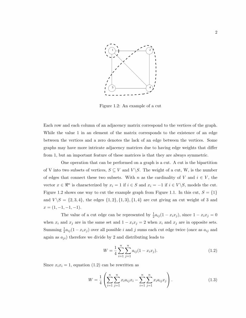
Figure 1.2: An example of a cut

Each row and each column of an adjacency matrix correspond to the vertices of the graph.

While the value 1 in an element of the matrix corresponds to the existence of an edge

between the vertices and a zero denotes the lack of an edge between the vertices. Some

graphs may have more intricate adjacency matrices due to having edge weights that differ

from 1, but an important feature of these matrices is that they are always symmetric.

One operation that can be performed on a graph is a cut. A cut is the bipartition

of V into two subsets of vertices, S ⊆ V and V \S. The weight of a cut, W, is the number

of edges that connect these two subsets. With n as the cardinality of V and i ∈ V , the

vector x ∈ <n is characterized by xi = 1 if i ∈ S and xi = −1 if i ∈ V \S, models the cut.

Figure 1.2 shows one way to cut the example graph from Figure 1.1. In this cut, S = {1}and V \S = {2, 3, 4}, the edges {1, 2}, {1, 3}, {1, 4} are cut giving an cut weight of 3 and

x = (1,−1,−1,−1).

The value of a cut edge can be represented by 12aij(1 − xixj), since 1 − xixj = 0

when xi and xj are in the same set and 1 − xixj = 2 when xi and xj are in opposite sets.

Summing 12aij(1− xixj) over all possible i and j sums each cut edge twice (once as aij and

again as aji) therefore we divide by 2 and distributing leads to

W =14

n∑i=1

n∑j=1

aij(1− xixj). (1.2)

Since xixi = 1, equation (1.2) can be rewritten as

W =14

n∑i=1

n∑j=1

xiaijxi −n∑

i=1

n∑j=1

xiaijxj

. (1.3)

3

43

21

Figure 1.3: An example of a max-cut

For a vector v, the Diag(v) is the diagonal matrix where the values of v are placed on the

main diagonal. And let e be the ones vector of dimension n. Then by the definition of

vector-matrix multiplication W = 14

(xtDiag(Ae)x− xtAx

). The laplacian of a graph, L,

is a matrix such that L = Diag(Ae) − A. Distributing the vectors, equation (1.3) is now

simplified to

W =14xtLx. (1.4)

The Laplacian of the example graph 1.1 is

L =

3 −1 −1 −1

−1 2 0 −1

−1 0 2 −1

−1 −1 −1 3

. (1.5)

A maximum cut is a cut that has the greatest weight for that graph. Figure 1.3

shows the max-cut of the graph in Figure 1.1. In this cut, S = {1, 4} and V \S = {2, 3}, the

edges {1, 2}, {1, 3}, {2, 4}, {3, 4} are cut giving an cut weight of 4 and x = (1,−1,−1, 1).

W ∗ = maxx∈{−1,1}n

14xtLx. (1.6)

Evaluating equation (1.6) is a discrete optimization problem known as the maximum cut

(max-cut) problem. The max-cut problem is known to be NP-complete (Crescenzi and

Kann [1]). In equation (1.6), the vector x has 2n possible discrete values. Since x and −x

are degenerate cuts, cutting the same edges but swapping set names, 2n−1 possibilities need

to be considered when evaluating equation (1.6). A common approach to solving discrete

optimization problems is the cutting plane approach discussed in Section 1.3.

4

1.2 Applications

1.2.1 Spin glasses

The Ising spin glass model of ferromagnetism uses electron spin to determine

the potential energy of an array of atoms. When these atoms are arranged in crystalline

structures a dominant spin direction can appear. The vector s ∈ {1,−1}n models the

electron spins of such a crystal, where si = 1 if it is parallel to the dominant direction and

si = −1 if it is anti-parallel. J is the matrix of spin interactions, frequently assumed to be

nearest neighbor. A value h is determined by the presence of an external magnetic field.

Therefore the hessian, H of the crystal is

H(s) = −n∑

i=1

n∑j=1

Ji,jsisj − hn∑

i=1

si (1.7)

(Hartmann and Rieger [2]). This model is an example where each i is a vertex and the

values of that si takes are the same as whether i ∈ S or i ∈ V \S. Introducing a dummy

vertex s0 lets us collapse the second summation in equation (1.7) into the first with J0,0 = 0

and Ji,0 = J0,i = h2 when i 6= 0.

H(s) = −n∑

i=0

n∑j=0

Ji,jsisj . (1.8)

The problem of finding the ground state energy of the model is then the same as finding

the following maximum,

maxs∈{1,−1}n

n∑i=0

n∑j=0

Ji,jsisj = maxs∈{1,−1}n

stJs. (1.9)

Comparing the right hand side of equation (1.9) and equation (1.6) shows that a solution

to the max-cut problem is a solution to the spin glass problem (Hartmann and Rieger [2]).

1.2.2 VLSI

Very large scale integration (VLSI) is the design and layout of integrated circuits.

The routing of wires occurs after the placement of circuit elements and after the placement

of nets which allow wires which would conflict to pass each other in different layers. One of

the objectives of routing is to minimize the number of locations where wires change layers

since this is accomplished with vias, small holes drilled into the chip, a process that both

5

risks breaking the chip and causes significant additional expense. Nets allow wires to pass

each other by establishing critical segments for each wire, areas where vias are not allowed.

Between nets, vias are allowed in what are called free segments.

A circuit is modeled with a graph where each vertex is a wire length in a critical

segment and there are two types of edges. The first type of edge, called a conflict edge,

connects vertices that represent wires that are crossing in the segment, i.e. segments in

conflict. The second type of edge, the free edge, connects critical wire segments according

to the free segments (Barahona et. al. [3]). A reduced graph is created by choosing a single

vertex within each critical segment to serve as a representative. Determining the layer of

some vertex forces all critically adjacent vertices into the opposing layer therefore once each

representative is known all other vertices are determined. The edge weights between these

representative segments are obtained by summing the number of free edges cut when the

representative vertices are in opposite layers and subtracting the number of free edges cut

when they are in the same layer.

The solving of the max-cut for this representative graph minimizes the number of

vias created for this circuit layout(Barahona et. al. [3]).

1.3 Cutting plane approach

1.3.1 Relaxations

The cutting plane approach solves difficult maximization problems by creating

and solving simpler problems, called relaxations. The feasible region for a relaxation must

contain the feasible region for the original problem. Furthermore, for any solution that is

feasible in the original problem, the objective value in the relaxation must be equal to or

greater than the objective value in the original problem (Wolsey [4]).

1.3.2 Cutting planes

Once a relaxation is solved to optimality, the optimal solution to the relaxation

is checked to see if it is feasible in the original problem. If the optimal relaxation solution

is not feasible then further steps are required. A new constraint(s) must be added to the

relaxation so that the current optimal relaxation solution is no longer feasible but all of the

original problems solutions remain feasible, this new constraint is called a cutting plane.

6

The problem of finding cutting planes, called the separation problem, is central to

the cutting plane approach. Problem specific solutions are available for some optimization

problems, including the max-cut problem. Once the separation problem is solved, there

is a new relaxation characterized by the prior relaxation and the new valid inequality(ies)

(Wolsey [4]).

1.3.3 Bounds

The optimal value of a relaxation is an upper bound on the optimal value of the

original maximization problem. Also, the objective value for any feasible solution is a lower

bound on the original optimal value. So, if the relaxation’s optimal solution is original

feasible and the bounds are equal then this solution is optimal in the original. The process

of solving relaxations, checking feasibility, and solving separation problems continues until

the optimal solution is found or the bounds are within any arbitrary ε > 0.

1.4 Semidefinite optimization

1.4.1 Conic optimization

The characteristics of a conic optimization problem can be shown by considering

the following problem.

max ctx

s.t. Bx = b

x ∈ K

(1.10)

where c ∈ <n, B ∈ <m×n, b ∈ <m, and K is a closed convex cone (Vandenberghe and Boyd

[5]).

1. The objective function and constraint equations in problem (1.10) are linear and are

expressed as an inner product or sum of inner products over the appropriate cones.

2. The variables are restricted to some closed, convex cone, K or a cartesian product of

such cones.

3. Every convex optimization problem (Sivaramakrishnan [6]) can be rewritten as a conic

optimization problem in the form (1.10).

7

4. When K = <n then problem (1.10) is a linear program.

The dual of a cone, K, is the cone such that K∗ = {u|utx ≥ 0, ∀x ∈ K}. If the

cone is a self-dual cone, i.e., K = K∗, then the dual of the optimization is as follows in

(1.11).

min bty

s.t. Bty + s = c

s ∈ K

(1.11)

(Ramana [7]).

Conic optimization problems are continuous optimization problems. And lend

themselves to analysis with duality theory and interior point solving methods (Zhang [8]).

1.4.2 Positive semidefinite cone

The general form for positive semidefinite programs, analogous to problem (1.10),

is

max C •X

s.t. Bi •X = bi, i = 1, . . . ,m

X � 0.

(1.12)

where the following definitions hold:

1. The inner product used for semidefinite optimization is the Frobenius inner product,

C •X =∑n

i=1

∑nj=1 CijXij .

2. The cone used for semidefinite optimization is the cone of symmetric matrices, i.e.,

X ∈ Sn = {Y ∈ <n×n|Y = Y t}, where Sn is the set of symmetric matrices of size n.

3. Instead of non-negativity constraints, as in linear optimization, positive semidefinite

optimization requires that X is positive semidefinite, X � 0. A matrix is positive

semidefinite if dtXd ≥ 0 for any vector d ∈ <n or, equivalently, when all of the

eigenvalues of X are greater than or equal to zero. The union of Sn and X � 0 is a

self-dual, pointed, closed, convex cone, Sn+.

8

Since the cone Sn+ is a self-dual, pointed, closed, convex cone the dual problem for

the primal problem (1.12) is written as

min bty

s.t.∑m

i=1 Biyi + S = C

S � 0.

(1.13)

1.5 Prior methods

Another way to represent the max-cut problem is

max xtLx

s.t. x2i = 1, i = 1, . . . , n.

(1.14)

Formulation (1.14) is a 0-1 quadratic program and is NP-complete, it does lead to this

straight forward relaxation,

max xtLx

s.t. xi ≤ 1, i = 1, . . . , n

xi ≥ −1, i = 1, . . . , n,

(1.15)

which is frequently used in branch and cut algorithms. This relaxation lends itself to a

rounding procedure where i ∈ S for all xi ≥ 0 and i ∈ V \S otherwise. This rounding

procedure gives a feasible solution whose expected objective value is of .5 times the optimal

value (Goemans and Williamson [9]).

1.6 Contribution and organization of thesis

This thesis proposes to solve the max-cut problem to optimization using semidef-

inite relaxations in a cutting plane algorithm. Chapter 2 will lay out the structure of the

algorithm and discuss our experimental set-up and the results we obtained from it. Section

2.1 gives a detailed overview of the cutting plane algorithm. The three major steps of this

algorithm are each discussed in their own section; the form and solution of the SDP relax-

ation of the max-cut problem in Section 2.2, Section 2.3 explains the Goemans-Williamson

rounding method and the corresponding strength of the bounds this method obtains, and

the separation oracle, which finds violated triangle inequalities, is discussed in Section 2.4.

Finally, we have implemented this cutting plane algorithm in MATLAB and the Section 2.5

9

discusses the setup and results of this implementation. We generated graphs of a given size

with each edge weight randomly chosen from a Bernoulli distribution with a probability

equal to the edge density. Our computational results with the algorithm are reported where

the number of vertices and the density of the edges vary between 5 to 45 and 0.1 to 1.0,

respectively. And a series of 50 runs with 30 vertices and an edge density of .5 were run to

give an approximation of the frequency of extremely difficult problems. We wrap things up

and discuss where can go forward in Section 2.6.

10

Chapter 2

Algorithm

2.1 Cutting plane algorithm for the max-cut problem

1. Initialize: From a given adjacency matrix, A, setup the variables: n = |A|, the

laplacian, L = Diag(Ae)− A from Section 1.1, and the constraint matrices eieti, i =

1, . . . , n, from Section 2.2. Also, initialize the block variable, blk, to indicate a semidef-

inite cone of size n.

2. Solve the SDP relaxation: Solve the SDP relaxation formulated in Section 2.2

using blk to inform SDPT-3, a primal-dual IPM software, of the size and type of the

current variables (Toh, Todd, and Tutuncu [10]).

3. Goemans-Williamson rounding heuristic: Use the rounding heuristic discussed

in Section 2.3 to find a feasible candidate solution. Repeat this 100 times keeping the

best candidate as s.

4. Separation oracle: Find violated inequalities using the separation oracle, Section

2.4. Update the current constraints to include the violated inequalities and blk to

indicate the new linear slack variables.

5. Check for optimality: Repeat steps 2 through 4 until the objective values of the

current candidate solution and SDP relaxation are within ε > 0 of each other or the

maximum number of iterations has been exceeded.

This framework is used by the m-script maxopt in Appendix A.1.

11

2.2 Semidefinite relaxation formulation of the max-cut prob-

lem

Recall the max-cut problem, from Section 1.1,

W ∗ = maxx∈{−1,1}n

14xtLx, (2.1)

where it was concluded that the solution to equation (2.1) can not be found efficiently. A

semidefinite relaxation of the max-cut problem can be formulated, to create this relaxation

the variables, objective, and constraints first need to be expressed as matrices. Changing

objective function (1.4) using the definitions of vector-matrix multiplication and the Frobe-

nius inner product, from Section 1.4.2, xtLx =∑

i

∑j xiLijxj = L • xxt, and let X = xxt.

Therefore, X � 0 and is rank one. Second, the constraint that x ∈ {1,−1}n must be also

be reformulated. Letting ei be the vector of size n whose values are zero except for element

i whose value is one, restate the constraint that xi ∈ {1,−1} as follows: 1 = xixi = xteietix.

Then, using the definition of the inner product again, xteietix = eie

ti •X = 1. Up until now

we have only rewritten the constraints in a different form, therefore the formulation (2.2)

is the max-cut problem and is NP-complete.

max L •X

s.t. eieti •X = 1, i = 1, . . . , n

X � 0

X is rank one.

(2.2)

Finally, relaxing the restriction that X is rank one, we are left with the semidefinite re-

laxation (2.3), which is not NP-complete and is efficiently solvable as discussed in Section

1.4.

maxX L •X

s.t. eieti •X = 1, i = 1, . . . , n

X � 0.

(2.3)

Solving this semidefinite program will give an X such that the value of L •X is an upper

bound on the optimal value of the max-cut problem. Furthermore, formulation (2.3) is

a stronger relaxation than the quadratic relaxation (1.15) in that it gives a lower upper

bound. Our implementation maxopt calls the routine avec and the solver sqlp from the

SDPT - 3 package, (Toh, Todd, and Tutuncu [10]), to solve our SDP relaxations.

12

Section 2.4 introduces new constraints and new variables to the formulation (2.3).

These constraints are of the form Bh •X +wh = 1, h = 1, . . . ,m, therefore future iterations

use

maxX, w L •X + 0tw

s.t. eieti •X = 1, i = 1, . . . , n

Bh •X + wh = 1, h = 1, . . . ,m

X � 0

w ≥ 0

(2.4)

as the relaxation to be solved by SDPT-3. Formulation (2.4) is a conic optimization problem

where X is in the positive semidefinite cone and w is in the linear cone. The solution to

this formulation also gives an upper bound on the max-cut problem.

2.3 Goemans-Williamson rounding

It is useful to be able to generate a feasible solution to an original discrete problem,

such as the max-cut, from the solution to a continuous relaxation, such as the semidefinite

relaxation of the max-cut. This is done with rounding methods, in particular Goemans-

Williamson rounding yields the best known polynomial time approximation using the fol-

lowing procedure:

1. The rounding procedure begins with a solved semidefinite relaxation and the corre-

sponding X. Cholesky factorization of X gives an upper triangular matrix, U , such

that X = U tU .

2. The rounding procedure then generates a random vector, r, of length n by generating

each component uniformly on the interval [−1, 1] and then normalizing. This results

in a random vector on the unit hypersphere.

3. For each i ∈ {1, . . . , n}, let ui be the ith column of U , then the feasible vector s is

formed by si = 1 if utir ≥ 0 and si = −1 otherwise (Goemans and Williamson [9]).

Recall from Section 1.1 that s models the cut where si = 1 if and only if i ∈ S and

i ∈ V \S otherwise. Also recall that the quadratic relaxation rounding in Section 1.5 gives

an expected objective value of .5 times the optimal value. Goemans-Williamson rounding

13

however gives a feasible s vector with an expected value of .878 times the optimal when the

edge weights are non-negative (Goemans and Williamson [9]).

The rounding procedure is very fast computationally and can sometimes produce

the optimal solution. The maxopt implementation calls the subroutine gwround in Ap-

pendix A.2 which uses the solution to the current semidefinite relaxation to solve the round-

ing procedure 100 times, letting s = max{stLs, stLs} with each new vector s. The vector s

is initialized as the zero vector before the first iteration of the cutting plane algorithm and

the current s is retained from the last iteration to the current iteration.

2.4 Separation oracle

The relaxation and rounding procedure will frequently leave a significant gap be-

tween the upper bound and the objective value associated with s. Cutting planes are used

to reduce the feasible space of the relaxation which results in a lower upper bound reducing

the gap and thereby show optimality. The inequalities that will be investigated are the

triangle inequalities, a subset of the hypermetric inequalities (Helmberg and Rendl [11]),

Xij + Xjk + Xik ≥ −1 (2.5)

and

Xij −Xjk −Xik ≥ −1. (2.6)

To show that one of the inequalities (2.5) or (2.6) is a cutting plane it must be

shown that all feasible solutions to the max-cut satisfy it and that the solution to the

relaxation, X, violates it.

To show that all feasible max-cut solutions satisfy the inequalities (2.5) and (2.6)

choose any three vertices, i, j, and k. In any feasible solution to the max-cut problem the

vertices i, j, and k are either all in the same set or one is in the set opposite the other two.

Using Xij = xixj , four cases need to be examined.

1. If all of the vertices are in the same set then Xij = Xjk = Xik = 1 so inequalities

(2.5) and (2.6) reduce to 3 ≥ −1 and −1 ≥ −1 respectively.

2. If i is in the set opposite the other two then Xij = Xik = −1 and Xjk = 1, which

leaves both two inequalities as −1 ≥ −1.

14

3. The case where j is in the opposite set from the other two follows identically from

case 2 by switching the roles of i and j.

4. Finally, when k is the vertex in a set opposite the other two then Xjk = Xik = −1

and Xij = 1, which leads inequality (2.5) to −1 ≥ −1 and (2.6) to 3 ≥ −1.

Since i,j, and k were arbitrarily chosen, any solution that is feasible to the max-cut problem

must satisfy the inequalities (2.5) and (2.6) for all possible combinations of i,j, and k.

The solution to the relaxation can be checked to see if, for any i, j, and k, it

satisfies the inequalities (2.5) and (2.6), which it does not necessarily. Once a particular

combination i, j, k, and an inequality are found to result in a violation these are used to

create a cutting plane.

Let a set of violated inequalities be indexed by h ∈ {1 . . . m} and let bh ∈ <n be a

vector whose components are zero except bhi, bhj

, and bhkwhich should be assigned 1 or -1

as follows:

Case 1: [bhi, bhj

, bhk] = [1, 1, 1]

Cases 2, 3, and 4: [bhi, bhj

, bhk] = [−1, 1, 1], [1,−1, 1], and [1, 1− 1], respectively.

(2.7)

Then letting Bh = bhbth,

2(BhijXij + Bhjk

Xjk + BhikXik) ≥ −2

Xii + Xjj + Xkk + 2(BhijXij + Bhjk

Xjk + BhikXik) ≥ 1 + 1 + 1− 2

X •Bh ≥ 1

(2.8)

by the definition of the Frobenius inner product and the violated inequality h. Finally,

introducing a slack variable, w ≥ 0, the new constraints to the current relaxation are of the

form:

X •Bh + wh = 1, h = 1..m. (2.9)

2.5 Computational results

2.5.1 Setup

Our implementation used three input arguments, the adjacency matrix, some ε > 0

to determine precision, and a maximum number of iterations. While coding the implemen-

tation, ε was compared with the absolute gap between the feasible solution value and upper

15

bound. Therefore, a value of 1 was used since the value of any feasible solution was integer

this guaranteed optimality when the upper bound was within 1. For the execution, a rela-

tive gap was used. This gap was obtained by dividing the absolute value of the absolute gap

by the absolute value of the current feasible objective value. A value of 10−3 was used for

when iterations were tested for convergence, this is considerably tighter than an absolute

gap of 1 for smaller graphs. The maximum number of iterations was left very large when

testing for time and convergence.

The separation oracle, Section 2.4, was executed with the following considerations.

For the first cut iteration, the floor(n5 ) = bn5 c cuts are used. For each other iteration j,

bn5 1.5jc cuts are used. Cuts were found exhaustively. Sets of three nodes were chosen

in bibliographic order, then the inequality (2.5) was checked and the inequality (2.6) was

checked three times, once for each prospective node k.

The three outputs of the m-script are the current objective value, the associated

feasible vector, and a flag indicating whether the program terminated due to exceeding the

maximum number of iterations or if ε > gap.

All of the computational results were obtained on a Dell ZEN 7 workstation with

IntelrCore(TM) 2 CPU 6600 @ 2.40 GHz and 2.39 GHz 2.00 GB of Ram, running Microsoft

Windows XP Professional.

2.5.2 Results

To gain a variety of results random graphs were generated with vertices from 5 to

45 at intervals of 5 and edge density, p, from 0 to 1 in increments of .1. For some instances

the semidefinite relaxation and Goemans Williamson rounding immediately resulted in an

optimal solution. These instances include all graphs with empty edge sets, all complete

graphs, and some of the smaller graphs.

The plot in Figure 2.1 shows the values displayed in Table 2.1 in a plot that reads

the table horizontally, so that vertices are on the x-axis and the processing time is the

y-axis. The time scale is logarithmic so that the different run times for the graphs with

small numbers of vertices are visible. The legend indicates which line corresponds to which

edge density. Here it can be clearly noted that neither an empty graph nor a complete one

are any trouble to solve for any size graph, and although an edge density of .1 initially lags

the other plots in complexity it too shows exponential growth once there are 35 vertices.

16

Table 2.1: The processing time of random graphsn 5 10 15 20 25 30 35 40 45

0.0 .0542 .0508 .0802 .0784 .1361 .0901 .1033 .1039 .15840.1 .0931 .1379 .1469 .1684 .2304 .6193 15.9422 27.2459 102.00720.2 .0879 .1265 .1472 .2781 8.0748 20.0286 14.9803 70.1951 510.71940.3 .0648 .1056 .1217 3.4711 1.8770 18.6100 50.9392 19.5079 89.17430.4 .1090 .1755 .3778 1.6119 13.5046 5.0821 93.0798 69.2865 334.06060.5 .1687 .1065 .1538 .1292 8.0891 18.7627 26.5226 68.0561 214.15440.6 .1217 .1092 .5658 4.5985 7.9049 7.2189 14.2534 154.1022 216.48470.7 .1215 .1157 .2177 4.5976 7.8223 19.1133 54.9289 71.0043 530.45470.8 .0917 .1135 .1373 9.9733 5.3391 19.0519 51.0602 33.9482 412.69970.9 .0753 .1228 .1279 1.8304 1.2458 7.4325 26.7003 74.1400 215.12681.0 .0838 .0828 .1048 .0867 .1244 .1168 .1026 .1162 .1446

5 10 15 20 25 30 35 40 4510-2

10-1

100

101

102

103

Nodes

Pro

cess

ing

Tim

e (s

econ

ds) (

Loga

ritm

ic s

cale

)

p = 0 p = .1 p =.2 p = .3 p = .4 p = .5 p = .6 p = .7 p =.8 p = .9 p = 1

Figure 2.1: A plot of run times versus number of vertices with edge density held constant

17

The growth rate of the run times is exponential, to explore this further an additional set of

runs was generated with vertices from 2 to 42 with an edge density of .5 was run. This new

series of runs, Figure 2.2, was fit very cleanly by the exponential curve, t = .0259e.2102n,

which is plotted with it.

0 5 10 15 20 25 30 35 40 4510-2

10-1

100

101

102

103Run times versus Nodes with an edge density of .5

nodes

time

(sec

onds

) (lo

garit

hmic

sca

le)

run times fit line

Figure 2.2: A plot of run times versus number of vertices with edge density = .5

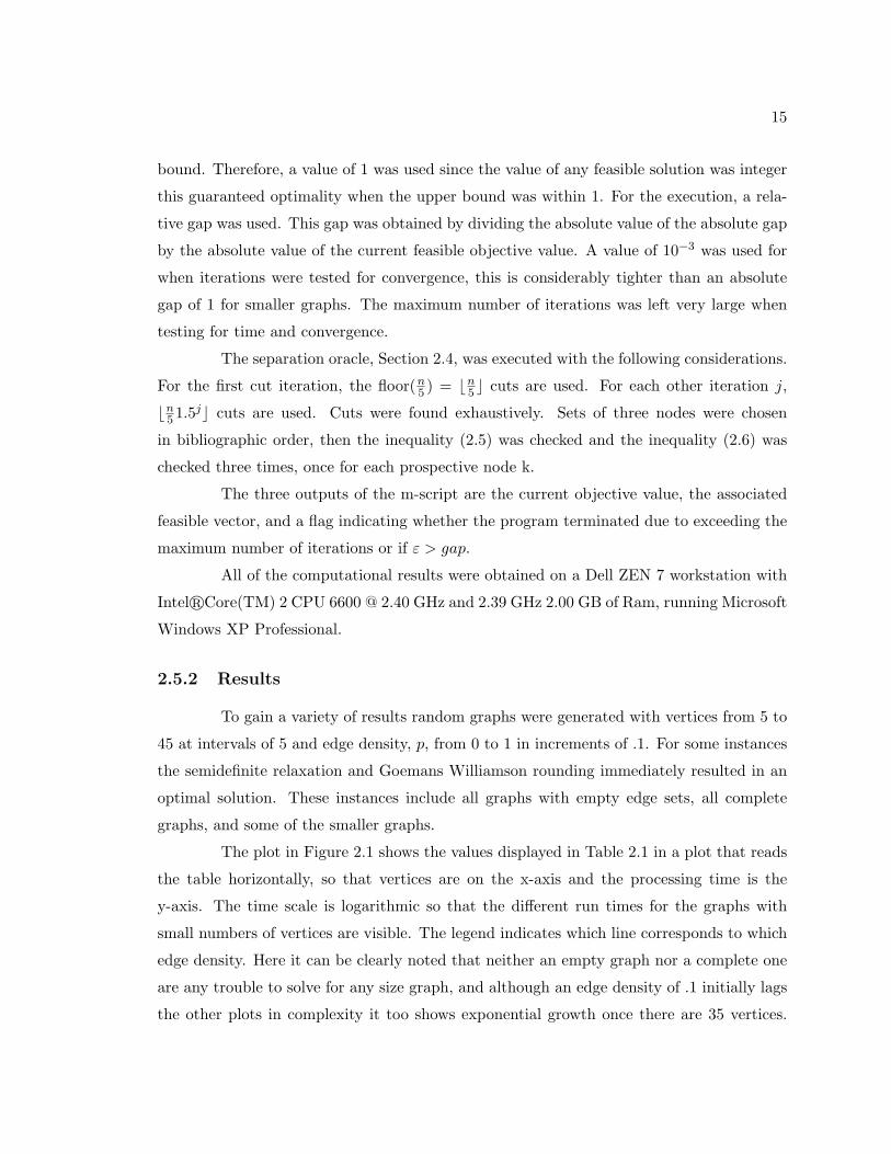
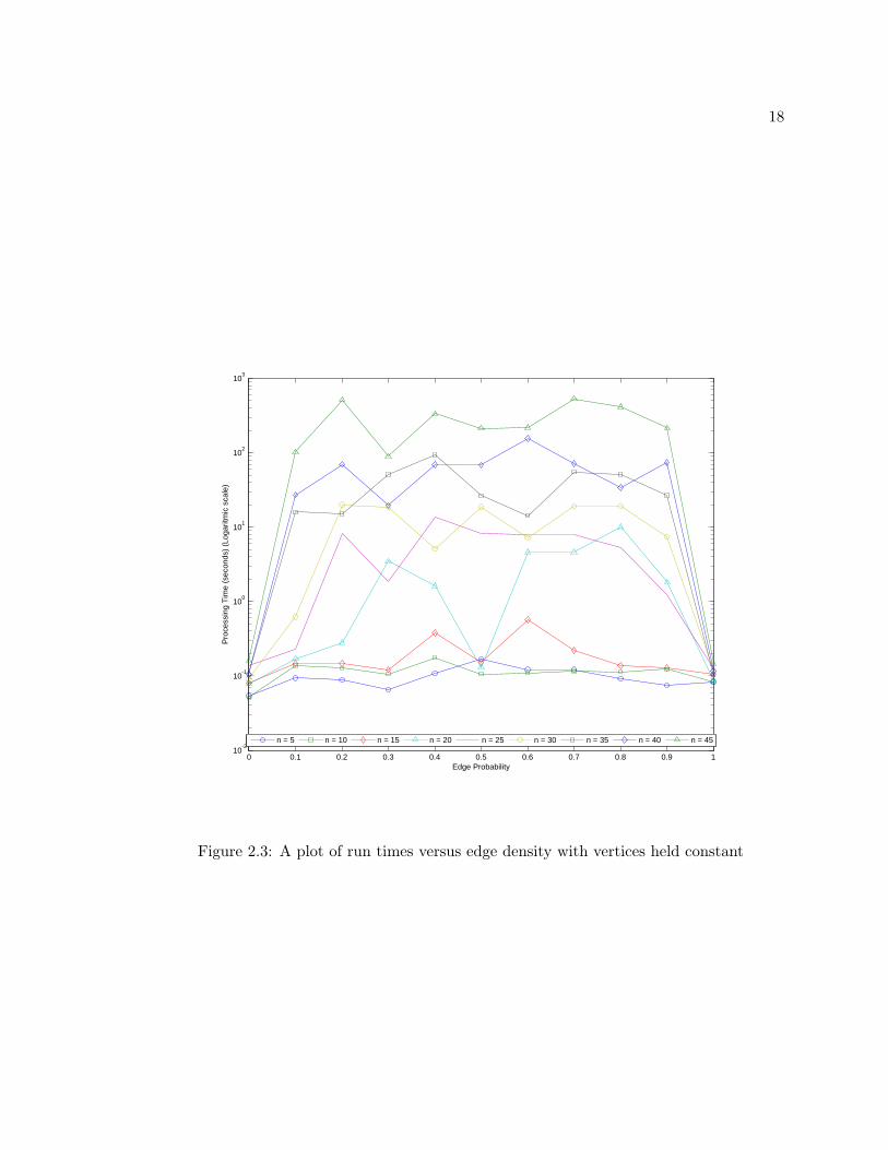
Table 2.1 can also be read vertically so that we can understand the relationship

between the edge density and the run times. This relationship is plotted in Figure 2.3

and as with Figure 2.1 the time scale is logarithmic so that the runs with few vertices are

distinguishable from each other. However, Figure 2.3 uses the edge density as the x-axis

and the different graph sizes are data sets as indicated by the legend. To get a better sense

of how well a quadratic function fits the times graphs of 25 edges were generated with edge

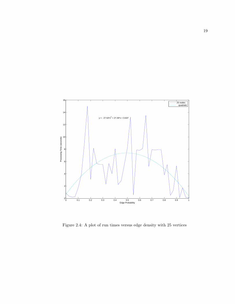
weights incrementing by steps of .025 and the results are plotted in Figure 2.4.

Fifty runs of graphs with 30 vertices and an edge density of .5 are displayed in

18

0 0.1 0.2 0.3 0.4 0.5 0.6 0.7 0.8 0.9 110-2

10-1

100

101

102

103

Edge Probability

Pro

cess

ing

Tim

e (s

econ

ds) (

Loga

ritm

ic s

cale

)

n = 5 n = 10 n = 15 n = 20 n = 25 n = 30 n = 35 n = 40 n = 45

Figure 2.3: A plot of run times versus edge density with vertices held constant

19

0 0.1 0.2 0.3 0.4 0.5 0.6 0.7 0.8 0.9 10

2

4

6

8

10

12

14

16

Edge Probability

Pro

cess

ing

Tim

e (s

econ

ds)

y = - 27.53*x2 + 27.26*x + 0.637

25 nodes quadratic

Figure 2.4: A plot of run times versus edge density with 25 vertices

20

0 10 20 30 40 50 60 70 800

2

4

6

8

10

12

14

16

18

20

Time (Seconds)

Run

s

Figure 2.5: A histogram of 50 runs with 30 vertices and an edge density = .5

21

the histogram in Figure 2.5. The mean of these runs is 19.2987 seconds and the standard

deviation is 13.2159 seconds. The 50 runs spanned from 1.0418 seconds to 73.8306 seconds

with a median of 18.4806 seconds.

2.6 Conclusions and future work

My approach to solving the max-cut problem to optimality using of semidefinite

programming in a cutting plane algorithm has shown some success. In particular, I have

been able to show optimality on examples with as many as 45 vertices. The separation

oracle showed that the triangle inequality cutting planes were plentiful, available in the

thousands for larger problems. The SDP solver was able to swiftly solve instances of the

initial problem while the addition of thousands of linear variables added complexity with

too little gain for the implementation to consistently work on larger instances.

For a graph with 25 vertices and an edge density of .5 the quadratic fit from Figure

2.4 predicts a time 7.38 seconds while the exponential fit from Figure 2.2 predicts a time of

4.96 seconds. The fit from Figure 2.2 predicts that the time to evaluate a 30 vertex graph

with .5 edge density is 14.20 seconds. While the median of 18.4806 seconds was obtained

from the 50 runs of a graph of this size. The differences in the run time predictions indicates

that these problems have highly variable complexity, which is corroborated by the standard

deviation of the fifty runs, 13.2159 seconds, being more than half of its mean, 19.2987. This

variability is also indicated by the presence of a single run of 30 vertices and p = .5 that

took 73.8306 seconds to solve, as indicated in Figure 2.5. This run time is more than 4

standard deviations above the mean.

The most interesting future refinements to the implementation are the use of other,

possibly tighter, problem specific cutting planes, the addition of a routine that would remove

cutting planes from the current relaxation that are very strongly satisfied, and the creation of

a branching routine that would use only a single additional constraint. The main advantage

that either of these would add is a lessened sensitivity to problem size since larger problems

require larger numbers of constraints to tighten them to optimality. The addition of tighter

cutting planes can be costly because of their complexity. The constraints to be removed

in the second option would be identified by the large corresponding slack variables, since

semidefinite optimization has strong duality while either the primal or dual problem has an

interior. The downside of this addition may be that same constraint needs to be added to

22

the formulation more than once since it was removed by an earlier iteration. The branching

routine would function by branching a single vector g where with each branch another gi

is forced to 1 or -1. This vector would give rise to a single additional constraint, ggt •X =

ggt • ggt so that each iteration would nearly as fast as the iteration before branching began.

The difficulty here would arise as the number of branches needed to be resolved could be

quite large.

23

Bibliography

[1] Pierluigi Crescenzi and Viggo Kann. A compilation of np optimization problems.

Technical Report SI/RR-95/02, University of Rome, 1995.

[2] A. K. Hartmann and H. Rieger, editors. New Optimization Algorithms in Physics,

chapter 3, pages 47–70. Wiley-VCH, 2004.

[3] Francisco Barahona, Martin Grotschel, Micheal Junger, and Gerhard Reinelt. An

application of combinatorial optimization to statistical physics and ciruit layout design.

Operations Research, 36(3):493–513, May-June 1988.

[4] Laurence A. Wolsey. Integer Programming. Wiley-interscience Publications, 1998.

[5] Lieven Vandenberghe and Stephen Boyd. Semidefinite programming. SIAM Review,

38:49–95, 1996.

[6] Kartik Sivaramakrishnan. Ma 796s: Convex optimization and interior point methods.

http://www4.ncsu.edu/ kksivara/ma796s/, 2007.

[7] Motakuri Ramana. An exact duality theory for semidefinite programming and its

complexity implications. Mathematical Programming, 77:129–162, 1997.

[8] Yin Zhang. On extending some primal-dual interior point methods for linear pro-

gramming to semidefinite programming. SIAM Journal on Optimization, 8:365–386,

1998.

[9] Michel Goemans and David Williamson. Improved approximation algorithms for maxi-

mum cut and satisfiability problems using semidefinite programming. Journal of ACM,

42(6):1115–1145, November 1995.

24

[10] Kim-Chuan Toh, Michael J. Todd, and Reha H. Tutuncu. Sdpt3 version 4.

http://www.math.nus.edu.sg/mattohkc/sdpt3.html, July 2006.

[11] Christoph Helmberg and Franz Rendl. Solving quadratic (0,1)-problems by semidefinite

programs and cutting planes. Mathematical Programming, 82:291–315, 1998.

25

Appendix A

Appendices

A Appendices

26

A.1 maxopt

function [objval,feasvec,flag,gap,progtrak,y] = maxopt(Adj,eps,maxiter)%MAXOPT - Returns the maximum cut for a graph.%INPUTS: Adj is the adjacency matrix of the graph to be cut.% eps is the gap which maxopt will accept as proof of optimality.% maxiter is the maximum number of iterations that will be% completed.%OUTPUTS: objval is the value of the objective function for the vector% feasvec.% feasvec is the best cut vector that maxopt has found.% flag is zero if maxopt ended because the gap was less than eps% and is one if the number of iterations exceeds maxiter.% gap is the gap between objval and the value of the most recent% semidefinite relaxation.% progtrak is a matrix containing the time of through the% iteration in the first column, the objective value of the% canidate solution at the end of the corresponding% iteration in the second column, and the objective value of% the semidefinite relaxation in the third column.% y is the dual variables of the semidefinite relaxation.

flag = 0;n = length(Adj); e = ones(n,1);C{1} = -(spdiags(Adj*e,0,n,n)-Adj)/4;b = e;blk{1,1} = ’s’; blk{1,2} = n;

A = cell(1,n);for k = 1:n; A{k} = sparse(k,k,1,n,n); end;

tic;Avec = svec(blk,A,ones(size(blk,1),1));[obj,X,y,Z] = sqlp(blk,Avec,C,b,[]);

dummyvec = zeros(n,1);[objval,feasvec] = gwround(X{1},C{1},dummyvec,0,n,100);toc;currenttime = toc;progtrak = [currenttime,objval,obj(1)];gapnum = abs(objval-obj(1));gapden = max(1,abs(obj(1)));gap = gapnum/gapden;if gap>eps

tic;

27

stormax = (n/5);iter = 1;[blk,A,C,b] = cutroutine(feasvec,blk,A,C,b,X,n,stormax);Avec = svec(blk,A,ones(size(blk,1),1));[obj,X,y,Z] = sqlp(blk,Avec,C,b,[]);[objval,feasvec] = gwround(X{1},C{1},feasvec,objval,n,100);toc;currenttime = currenttime + toc;progtrak = [progtrak;currenttime, objval, obj(1)];gapnum = abs(objval-obj(1));gapden = max(1,abs(obj(1)));gap = gapnum/gapden;while gap>eps && iter <= maxiter;

tic;stormax = stormax*1.5;iter = iter + 1;[blk,A,C,b] = cutroutine(feasvec,blk,A,C,b,X,n,stormax);Avec = svec(blk,A,ones(size(blk,1),1));[obj,X,y,Z] = sqlp(blk,Avec,C,b,[]);[objval,feasvec] = gwround(X{1},C{1},feasvec,objval,n,100);toc;currenttime = currenttime + toc;progtrak = [progtrak;currenttime, objval, obj(1)];gapnum = abs(objval-obj(1));gapden = max(1,abs(obj(1)));gap = gapnum/gapden;

endendif iter >= maxiter

flag = 1;end%branchroutineend

28

A.2 gwround

function [feasval,feasvec] = gwround(X,C,feasvec,feasval,n,iter)%GWROUND - This subroutine does Goemans-Williamson rounding iter times and chooses the%best vector and it’s objective to pass back.%INPUTS: X is the current solution to the relaxation.% C is the objective coefficient.% feasvec is the current canidate solution.% feasval is the objective value of the current canidate.% n is the size of the graph to be cut.% iter is the number of times that the rounding proceedure with% be repeated.%OUTPUTS: both feasval and feasvec are updates to contain the best% canidate so far.V = chol(X);vi = zeros(n,1);for k = 1:iter

r = randn(n,1);r = r/norm(r);for j = 1:n

if V(:,j)’*r >=0vi(j,1) = 1;

elsevi(j,1) = -1;

endendif vi’*C*vi < feasval

feasvec = vi;feasval = feasvec’*C*feasvec;

endend

29

A.3 cutroutine

function [blk,A,C,rhs] = cutroutine(canidate,blk,A,C,rhs,X,n,stormax)%CUTROUTINE returns a constraint set for maxopt updated with cuts%[blk,A,C,rhs] = cutroutine(canidate,blk,A,C,rhs,X,n,stormax)%INPUTS: canidate is the current best feasible solution to the max-cut% problem.% blk is the array of current variables for the SDP solver.% A is the array of constraint coefficients.% C is the array of objective function coefficients.% rhs is the vector of the values for the right hand side of the% constraints.% X is the solution to the current relaxation% n is the size of the graph being cut% stormax is the maximum number of cutting planes to be added% this iteration.%OUTPUTS: All of the outputs are updates of their inputs.storage =’’;

%find the first valid inequalities that bound the space to the current%canidate solutionfor i = 1:n-2

for j = i+1:n-1for k = j+1:n

b = zeros(n,1);b(i) = canidate(i);b(j) = canidate(j);b(k) = canidate(k);if isempty(storage)

if b’*X{1}*b < 1storage = b;

endelseif size(storage,2)<stormax;

if b’*X{1}*b < 1storage = [storage,b];

endend

endend

end

%find first remaining valid inequalitiesfor i = 1:n-2

for j = i+1:n-1for k = j+1:n

30

for q = 1:4b = zeros(n,1);if q == 1

b(i,1) = 1; b(j,1) = 1; b(k,1) = 1;elseif q == 2

b(i,1) = -1; b(j,1) = 1; b(k,1) = 1;elseif q==3

b(i,1) = 1; b(j,1) = -1; b(k,1) = 1;else

b(i,1) = 1; b(j,1) = 1; b(k,1) = -1;endif b’*X{1}*b < 1 && abs(b’*canidate) ~= 3

if isempty(storage)storage = b;

elseif size(storage,2)<stormax;storage = [storage,b];

endend

endend

endend

%Adjust blk (Find/create linear block, increase size appropriately)markl = 0;for lu = 1:size(blk,1)

if blk{lu,1}==’l’markl = lu;

endendif markl == 0

markl = size(blk,1)+1;blk{markl,1} = ’l’;blk{markl,2} = 0;

endm = size(storage,2);v = blk{markl,2};p = v + m;blk{markl,2} = p;

%Adjust A (Ensure new variables don’t impact prior constraints, create new%mixed sdp linear constraints)r = size(A,2);for s = 1:r

31

A{markl,s}(v+1:p,:) = zeros(m,1);endfor t = 1:m;

for u = 1:size(blk,1)if u == markl

A{u,t+r} = [zeros(t-1+v,1); -1; zeros(p-(t+v),1)];elseif blk{u,1} == ’s’

if blk{u,2} == nA{u,t+r} = storage(:,t)*storage(:,t)’;

elseA{u,t+r} = zeros(blk{u,2},blk{u,2});

endelse

A{u,t+r} = zeros(blk{u,2},1);end

endend

%Adjust C and rhs (New slacks get zeros in objective function, New%constraints set equal 1)C{markl}(v+1:p,:) = zeros(m,1);rhs = [rhs;ones(m,1)];