abstract of ece georgia institute of technology [email protected] hongyuan zha college of...

A Dirichlet Mixture Model of Hawkes Processes forEvent Sequence Clustering

Hongteng Xu∗School of ECE

Georgia Institute of [email protected]

Hongyuan ZhaCollege of Computing

Georgia Institute of [email protected]

Abstract

How to cluster event sequences generated via different point processes is an inter-esting and important problem in statistical machine learning. To solve this problem,we propose and discuss an effective model-based clustering method based on anovel Dirichlet mixture model of a special but significant type of point processes —Hawkes process. The proposed model generates the event sequences with differentclusters from the Hawkes processes with different parameters, and uses a Dirichletdistribution as the prior distribution of the clusters. We prove the identifiabilityof our mixture model and propose an effective variational Bayesian inferencealgorithm to learn our model. An adaptive inner iteration allocation strategy isdesigned to accelerate the convergence of our algorithm. Moreover, we investigatethe sample complexity and the computational complexity of our learning algorithmin depth. Experiments on both synthetic and real-world data show that the clus-tering method based on our model can learn structural triggering patterns hiddenin asynchronous event sequences robustly and achieve superior performance onclustering purity and consistency compared to existing methods.

1 Introduction

In many practical situations, we need to deal with a huge amount of irregular and asynchronoussequential data. Typical examples include the viewing records of users in an IPTV system, theelectronic health records of patients in hospitals, among many others. All of these data are so-calledevent sequences, each of which contains a series of events with different types in the continuous timedomain, e.g., when and which TV program a user watched, when and which care unit a patient istransferred to. Given a set of event sequences, an important task is learning their clustering structurerobustly. Event sequence clustering is meaningful for many practical applications. Take the previoustwo examples: clustering IPTV users according to their viewing records is beneficial to the programrecommendation system and the ads serving system; clustering patients according to their healthrecords helps hospitals to optimize their medication resources.

Event sequence clustering is very challenging. Existing work mainly focuses on clustering syn-chronous (or aggregated) time series with discrete time-lagged observations [19, 23, 40]. Eventsequences, on the contrary, are in the continuous time domain, so it is difficult to find a universal andtractable representation for them. A potential solution is constructing features of event sequences viaparametric [22] or nonparametric [18] methods. However, these feature-based methods have a highrisk of overfitting because of the large number of parameters. What is worse, these methods actuallydecompose the clustering problem into two phases: extracting features and learning clusters. As aresult, their clustering results are very sensitive to the quality of learned (or predefined) features.

∗Corresponding author.

31st Conference on Neural Information Processing Systems (NIPS 2017), Long Beach, CA, USA.

arX

iv:1

701.

0917

7v5

[cs

.LG

] 2

1 Se

p 20

17

To make concrete progress, we propose a Dirichlet Mixture model of Hawkes Processes (DMHPfor short) and study its performance on event sequence clustering in depth. In this model, the eventsequences belonging to different clusters are modeled via different Hawkes processes. The priorsof the Hawkes processes’ parameters are designed based on their physically-meaningful constraints.The prior of the clusters is generated via a Dirichlet distribution. We propose a variational Bayesianinference algorithm to learn the DMHP model in a nested Expectation-Maximization (EM) framework.In particular, we introduce a novel inner iteration allocation strategy into the algorithm with the helpof open-loop control theory, which improves the convergence of the algorithm. We prove the localidentifiability of our model and show that our learning algorithm has better sample complexity andcomputational complexity than its competitors.

The contributions of our work include: 1) We propose a novel Dirichlet mixture model of Hawkes pro-cesses and demonstrate its local identifiability. To our knowledge, it is the first systematical researchon the identifiability problem in the task of event sequence clustering. 2) We apply an adaptive inneriteration allocation strategy based on open-loop control theory to our learning algorithm and showits superiority to other strategies. The proposed strategy achieves a trade-off between convergenceperformance and computational complexity. 3) We propose a DMHP-based clustering method. Itrequires few parameters and is robust to the problems of overfitting and model misspecification,which achieves encouraging clustering results.

2 Related Work

A temporal point process [4] is a random process whose realization consists of an event sequence(ti, ci)Mi=1 with time stamps ti ∈ [0, T ] and event types ci ∈ C = 1, ..., C. It can be equivalentlyrepresented as C counting processes Nc(t)Cc=1, where Nc(t) is the number of type-c eventsoccurring at or before time t. A way to characterize point processes is via the intensity functionλc(t) = E[dNc(t)|HCt ]/dt, where HCt = (ti, ci)|ti < t, ci ∈ C collects historical events of alltypes before time t. It is the expected instantaneous rate of happening type-c events given the history,which captures the phenomena of interests, i.e., self-triggering [13] or self-correcting [45].

Hawkes Processes. A Hawkes process [13] is a kind of point processes modeling complicated eventsequences in which historical events have influences on current and future ones. It can also be viewedas a cascade of non-homogeneous Poisson processes [8, 35]. We focus on the clustering problem ofthe event sequences obeying Hawkes processes because Hawkes processes have been proven to beuseful for describing real-world data in many applications, e.g., financial analysis [1], social networkanalysis [3, 52], system analysis [22], and e-health [30, 43]. Hawkes processes have a particular formof intensity:

λc(t) = µc +∑C

c′=1

∫ t

0

φcc′(s)dNc′(t− s), (1)

where µc is the exogenous base intensity independent of the history while∑Cc′=1

∫ t0φcc′(s)dNc′(t−s)

the endogenous intensity capturing the peer influence. The decay in the influence of historical type-c′events on the subsequent type-c events is captured via the so-called impact function φcc′(t), which isnonnegative. A lot of existing work uses predefined impact functions with known parameters, e.g.,the exponential functions in [29,51] and the power-law functions in [50]. To enhance the flexibility, anonparametric model of 1-D Hawkes process was first proposed in [16] based on ordinary differentialequation (ODE) and extended to multi-dimensional case in [22, 52]. Another nonparametric modelis the contrast function-based model in [30], which leads to a Least-Squares (LS) problem [7].A Bayesian nonparametric model combining Hawkes processes with infinite relational model isproposed in [3]. Recently, the basis representation of impact functions was used in [6,15,42] to avoiddiscretization.

Sequential Data Clustering and Mixture Models. Traditional methods mainly focus on clusteringsynchronous (or aggregated) time series with discrete time-lagged variables [19, 23, 40]. Thesemethods rely on probabilistic mixture models [47], extracting features from sequential data andthen learning clusters via a Gaussian mixture model (GMM) [25, 28]. Recently, a mixture modelof Markov chains is proposed in [21], which learns potential clusters from aggregate data. Forasynchronous event sequences, most of the existing clustering methods can be categorized into feature-based methods, clustering event sequences from learned or predefined features. Typical examples

2

include the Gaussian process-base multi-task learning method in [18] and the multi-task multi-dimensional Hawkes processes in [22]. Focusing on Hawkes processes, the feature-based mixturemodels in [5, 17, 48] combine Hawkes processes with Dirichlet processes [2, 37]. However, thesemethods aim at modeling clusters of events or topics hidden in event sequences (i.e., sub-sequenceclustering), which cannot learn clusters of event sequences. To our knowledge, the model-basedclustering method for event sequences has been rarely considered.

3 Proposed Model

3.1 Dirichlet Mixture Model of Hawkes Processes

Given a set of event sequences S = snNn=1, where sn = (ti, ci)Mni=1 contains a series of events

ci ∈ C = 1, ..., C and their time stamps ti ∈ [0, Tn], we model them via a mixture model ofHawkes processes. According to the definition of Hawkes process in (1), for the event sequencebelonging to the k-th cluster its intensity function of type-c event at time t is

λkc (t) = µkc +∑

ti<tφkcci(t− ti) = µkc +

∑ti<t

∑D

d=1akccidgd(t− ti), (2)

where µk = [µkc ] ∈ RC+ is the exogenous base intensity of the k-th Hawkes process. Following thework in [42], we represent each impact function φkcc′(t) via basis functions as

∑d a

kcc′dgd(t − ti),

where gd(t) ≥ 0 is the d-th basis function and Ak = [akcc′d] ∈ RC×C×D0+ is the coefficient tensor.Here we use Gaussian basis function, and their number D can be decided automatically using thebasis selection method in [42].

In our mixture model, the probability of the appearance of an event sequence s is

p(s; Θ) =∑

kπkHP(s|µk,Ak), HP(s|µk,Ak) =

∏iλkci(ti) exp

(−∑

c

∫ T

0

λkc (s)ds). (3)

Here πk’s are the probabilities of clusters and HP(s|µk,Ak) is the conditional probability of theevent sequence s given the k-th Hawkes process, which follows the intensity function-based definitionin [4]. According to the Bayesian graphical model, we regard the parameters of Hawkes processes,µk,Ak, as random variables. For µk’s, we consider its positiveness and assume that they obeyC ×K independent Rayleigh distributions. ForAk’s, we consider its nonnegativeness and sparsityas the work in [22, 42, 51]) did, and assume that they obey C ×C ×D ×K independent exponentialdistributions. The prior of cluster is a Dirichlet distribution. Therefore, we can describe the proposedDirichlet mixture model of Hawkes process in a generative way as

π ∼ Dir(α/K, ..., α/K), k|π ∼ Category(π),

µ ∼ Rayleigh(B), A ∼ Exp(Σ), s|k,µ,A ∼ HP(µk,Ak),

Here µ = [µkc ] ∈ RC×K+ andA = [akcc′d] ∈ RC×C×D×K0+ are parameters of Hawkes processes, andB = [βkc ],Σ = [σkcc′d] are hyper-parameters. Denote the latent variables indicating the labels ofclusters as matrix Z ∈ 0, 1N×K . We can factorize the joint distribution of all variables as2

p(S,Z,π,µ,A) = p(S|Z,µ,A)p(Z|π)p(π)p(µ)p(A), where

p(S|Z,µ,A) =∏

n,kHP(sn|µk,Ak)znk , p(Z|π) =

∏n,k

(πk)znk ,

p(π) = Dir(π|α), p(µ) =∏

c,kRayleigh(µkc |βkc ), p(A) =

∏c,c′,d,k

Exp(akcc′d|σkcc′d).

(4)

Our mixture model of Hawkes processes are different from the models in [5, 17, 48]. Those modelsfocus on the sub-sequence clustering problem within an event sequence. The intensity function is aweighted sum of multiple intensity functions of different Hawkes processes. Our model, however,aims at finding the clustering structure across different sequences. The intensity of each event isgenerated via a single Hawkes process, while the likelihood of an event sequence is a mixture oflikelihood functions from different Hawkes processes.

2Rayleigh(x|β) = xβ2 e− x2

2β2 , Exp(x|σ) = 1σe−

xσ , x ≥ 0.

3

3.2 Local Identifiability

One of the most important questions about our mixture model is whether it is identifiable or not.According to the definition of Hawkes process and the work in [26, 31], we can prove that our modelis locally identifiable. The proof of the following theorem is given in the supplementary file.Theorem 3.1. When the time of observation goes to infinity, the mixture model of the Hawkes pro-cesses defined in (3) is locally identifiable, i.e., for each parameter point Θ = vec

([π1 ... πK

θ1 ... θK

]),

where θk = µk,Ak ∈ RC+ × RC×C×D0+ for k = 1, ..,K, there exists an open neighborhood of Θcontaining no other Θ′ which makes p(s; Θ) = p(s; Θ′) holds for all possible s.

4 Proposed Learning Algorithm

4.1 Variational Bayesian Inference

Instead of using purely MCMC-based learning method like [29], we propose an effective variationalBayesian inference algorithm to learn (4) in a nested EM framework. Specifically, we consider avariational distribution having the following factorization:

q(Z,π,µ,A) = q(Z)q(π,µ,A) = q(Z)q(π)∏

kq(µk)q(Ak). (5)

An EM algorithm can be used to optimize (5).

Update Responsibility (E-step). The logarithm of the optimized factor q∗(Z) is approximated as

log q∗(Z) = Eπ[log p(Z|π)] + Eµ,A[log p(S|Z,µ,A)] + C

=∑

n,kznk

(E[log πk] + E[log HP(sn|µk,Ak)]

)+ C

=∑

n,kznk

(E[log πk] + E[

∑ilog λkci(ti)−

∑c

∫ Tn

0

λkc (s)ds])

+ C

≈∑

n,kznk

(E[log πk] +

∑i

(logE[λkci(ti)]−

Var[λkci(ti)]2E2[λkci(ti)]

)−∑

cE[

∫ Tn

0

λkc (s)ds])

︸︷︷︸ρnk

+C.

where C is a constant and Var[·] represents the variance of random variable. Each term E[log λkc (t)]

is approximated via its second-order Taylor expansion logE[λkc (t)] − Var[λkc (t)]2E2[λkc (t)]

[38]. Then, theresponsibility rnk is calculated as

rnk = E[znk] = ρnk/(∑

jρnj). (6)

Denote Nk =∑n rnk for all k’s.

Update Parameters (M-step). The logarithm of optimal factor q∗(π,µ,A) is

log q∗(π,µ,A)

=∑

klog(p(µk)p(Ak)) + EZ [log p(Z|π)] + log p(π) +

∑n,k

rnk log HP(sn|µk,Ak) + C.

We can estimate the parameters of Hawkes processes via:

µ, A = arg maxµ,A log(p(µ)p(A)) +∑

n,krnk log HP(sn|µk,Ak). (7)

Following the work in [42, 48, 51], we need to apply an EM algorithm to solve (7) iteratively. Aftergetting optimal µ and A, we update distributions as

Σk = Ak, Bk =√

2/πµk. (8)

Update The Number of Clusters K. When the number of clusters K is unknown, we initialize Krandomly and update it in the learning phase. There are multiple methods to update the number of

4

20 40 60 80 100The number of inner iterations

3.44

3.46

3.48

3.5

Neg

ativ

e Lo

g-lik

elih

ood

#104 2 Clusters


5.1

5.15

5.2

Neg

ativ

e Lo

g-lik

elih

ood

#104 3 Clusters


7.1

7.2

7.3

7.4

7.5

Neg

ativ

e Lo

g-lik

elih

ood

#104 4 Clusters


8.3

8.4

8.5

8.6

Neg

ativ

e Lo

g-lik

elih

ood

#104 5 Clusters

Increasing Constant Decreasing OpenLoop BayesOpt

(a) Random Sparse Coefficients


4.12

4.14

4.16

4.18

4.2

4.22

Neg

ativ

e Lo

g-lik

elih

ood

#104 2 Cluster


6.9

7

7.1

7.2

7.3N

egat

ive

Log-

likel

ihoo

d#104 3 Cluster


8.2

8.25

8.3

8.35

8.4

Neg

ativ

e Lo

g-lik

elih

ood

#104 4 Cluster


1

1.01

1.02

1.03

1.04

Neg

ativ

e Lo

g-lik

elih

ood

#105 5 Cluster

Increasing Constant Decreasing OpenLoop BayesOpt

(b) Blockwise Sparse Coefficients

Figure 1: Comparison for various inner iteration allocation strategies on different synthetic data sets.Each curve is the average of 5 trials’ results. In each trial, total 100 inner iterations are applied. Theincreasing (decreasing) strategy changes the number of inner iterations from 2 to 8 (from 8 to 2). Theconstant strategy fixes the number to 5.

clusters. Regrading our Dirichlet distribution as a finite approximation of a Dirichlet process, we seta large initial K as the truncation level. A simple empirical method is discarding the empty cluster(i.e., Nk = 0) and merging the cluster with Nk smaller than a threshold Nmin in the learning phase.Besides this, we can apply the MCMC in [11, 49] to update K via merging or splitting clusters.

Repeating the three steps above, our algorithm maximizes the log-likelihood function (i.e., thelogarithm of (4)) and achieves optimal Σ,B accordingly. Both the details of our algorithm and itscomputational complexity are given in the supplementary file.

4.2 Inner Iteration Allocation Strategy and Convergence Analysis

Our algorithm is in a nested EM framework, where the outer iteration corresponds to the loop ofE-step and M-step and the inner iteration corresponds to the inner EM in the M-step. The runtime ofour algorithm is linearly proportional to the total number of inner iterations. Given fixed runtime(or the total number of inner iterations), both the final achievable log-likelihood and convergencebehavior of the algorithm highly depend on how we allocate the number of inner iterations acrossthe outer iterations. In this work, we test three inner iteration allocation strategies. The firststrategy is heuristic, which fixes, increases, or decreases the number of inner iterations as the outeriteration progresses. Compared with constant inner iteration strategy, the increasing or decreasingstrategy might improve the convergence of algorithm [9]. The second strategy is based on open-loopcontrol [27]: in each outer iteration, we compute objective function via two methods respectively— updating parameters directly (i.e., continuing current M-step and going to next inner iteration) orfirst updating responsibilities and then updating parameters (i.e., going to a new loop of E-step andM-step and starting a new outer iteration). The parameters corresponding to the smaller negativelog-likelihood are preserved. The third strategy is applying Bayesian optimization [33,36] to optimizethe number of inner iterations per outer iteration via maximizing the expected improvement.

We apply these strategies to 8 synthetic data sets and visualize their impacts on the convergence of ouralgorithm in Fig. 1. All the data sets are generated by the Hawkes processes with sparse coefficientsA. In the first four data sets, the nonzero elements in A are distributed randomly, and the numberof clusters increases from 2 to 5. In the last four data sets, each slide of Ak, k = 1, ...,K, contain

5


2.37

2.38

2.39

2.4

2.41

2.42

Neg

ativ

e Lo

g-lik

elih

ood

#105

IncreasingConstantDecreasing

200 400 600 800 1000Indices of samples

0

0.2

0.4

0.6

0.8

1

Res

pons

ibilit

y

Increasing

Ground Truth rn (15 Inner Iter.) E(rn) (15 Inner Iter.)


0

0.2

0.4

0.6

0.8

1

Res

pons

ibilit

y

Constant


0

0.2

0.4

0.6

0.8

1

Res

pons

ibilit

y

Decreasing

Figure 2: The data contain 200 event sequences generated via two 5-dimensional Hawkes processes.The black line is the ground truth. The red dots are responsibilities after 15 inner iterations, and thered line is their average.

several all-zero columns and rows (i.e. blockwise sparse tensor). In Fig. 1, we can find that theopen-loop control strategy and the Bayesian optimization strategy obtain comparable performanceon the convergence of algorithm. Both of them outperform heuristic strategies (i.e., increasing,decreasing and fixing the number of inner iterations per outer iteration), which reduce the negativelog-likelihood more rapidly and reach lower value finally. Although adjusting the number of inneriterations via different methodologies, both these two strategies tend to increase the number of inneriterations w.r.t. the number of outer iterations. In the beginning of algorithm, the open-loop controlstrategy updates responsibilities frequently, and similarly, the Bayesian optimization strategy assignssmall number of inner iterations. The heuristic strategy that increasing the number of inner iterationsfollows the same tendency, and therefore, is just slightly worse than the open-loop control and theBayesian optimization. This phenomenon is because the estimated responsibility is not reliable inthe beginning. Too many inner iterations at that time might make learning results fall into bad localoptimums.

Fig. 2 further verifies our explanation. With the help of the increasing strategy, most of the responsi-bilities converge to the ground truth with high confidence after just 15 inner iterations, because theresponsibilities has been updated over 5 times. On the contrary, the responsibilities corresponding tothe constant and the decreasing strategies have more uncertainty — many responsibilities are around0.5 and far from the ground truth.

Based on the analysis above, the increasing allocation strategy indeed improves the convergenceof our algorithm, and the open-loop control and the Bayesian optimization are superior to othercompetitors. Because the computational complexity of the open-loop control is much lower than thatof the Bayesian optimization, in the following experiments, we apply open-loop control strategy toour learning algorithm.

4.3 Computational Complexity and Acceleration

Given N training sequences of C-dimensional Hawkes processes, each of which contains I events,we represent impact functions by D basis functions and set the maximum number of clusters tobe K. In the worst case, the computational complexity per iteration of our learning algorithm isO(KDNI3C2). Fortunately, the exponential prior of tensorA corresponds to a sparse regularizer.In the learning phase, we can ignore the computations involving the elements close to zero to reducethe computational complexity. If the number of nonzero elements in each Ak is comparable toC, then the computational complexity of our algorithm will be O(KDNI2C). Additionally, theparallel computing techniques can also be applied to further reduce the runtime of our algorithm.Note that the learning algorithm of MMHP discretizes each impact function into L points andestimates them via finite element analysis. The low-rank regularizer is imposed on its parameters.Therefore, its computational complexity per iteration is O(NI(I2C2 + L(C + I)) +C3). Similarly,when the parameters of each Hawkes process is sparse, its computational complexity will reduce toO(NI(IC+L(C+I))+C2). The first partO(NI(IC+L(C+I))) corresponds to the ODE-basedparameter updating while the second part O(C2) corresponds to the soft-thresholding of parameters.According to the setting in [22, 52], generally L I . Therefore, the computational complexity ofour algorithm is superior to that of MMHP, especially in high dimensional cases (i.e., large C).

6

Algorithm 1 Learning DMHP1: Input: S = snNn=1, the maximum number of clusters K, the maximum number of iteration I .2: Output: Optimal parameters of model, α, Σ, and B.3: Initialize α, Σ,B and [rnk] randomly, i = 0.4: repeat5: Just M-step:6: Given [rnk], update µ(1), A(1) via (15), calculate negative log-likelihood L(1).7: A loop of E-step and M-step:8: Given α,Σ,B, update responsibility via (6), denoted as [r2

nk] .9: Given [r2

nk], update µ(2), A(2) via (15), calculate negative log-likelihood L(2).10: If L(1) < L(2)

11: Given µ(1), A(1), update Σ,B via (8).12: Else13: Update [rnk] via [r

(2)nk ].

14: Given [rnk], µ(2), A(2), update α, Σ,B via (8).15: End16: Merge or split clusters and update Σ,B via MCMC.17: i = i+ 1.18: until i = I19: α = α, Σ = Σ, and B = B.

80 Events per Sequence

0.1 0.2 0.3 0.4Sample Percentage of Minor Cluster

0.2

0.4

0.6

0.8

1

1.2

1.4

1.6

1.8

Dis

tanc

e be

twee

n C

ente

rs



0.2

0.4

0.6

0.8

1

1.2

1.4

1.6

1.8

Dis

tanc

e be

twee

n C

ente

rs



0.2

0.4

0.6

0.8

1

1.2

1.4

1.6

1.8

Dis

tanc

e be

twee

n C

ente

rs



0.2

0.4

0.6

0.8

1

1.2

1.4

1.6

1.8

Dis

tanc

e be

twee

n C

ente

rs



0.2

0.4

0.6

0.8

1

1.2

1.4

1.6

1.8

Dis

tanc

e be

twee

n C

ente

rs

0.2

0.3

0.4

0.5

0.6

0.7

0.8

0.9



0.2

0.4

0.6

0.8

1

1.2

1.4

1.6

1.8

Dis

tanc

e be

twee

n C

ente

rs

(a) MMHP+DPGMM



0.2

0.4

0.6

0.8

1

1.2

1.4

1.6

1.8

Dis

tanc

e be

twee

n C

ente

rs



0.2

0.4

0.6

0.8

1

1.2

1.4

1.6

1.8

Dis

tanc

e be

twee

n C

ente

rs



0.2

0.4

0.6

0.8

1

1.2

1.4

1.6

1.8

Dis

tanc

e be

twee

n C

ente

rs



0.2

0.4

0.6

0.8

1

1.2

1.4

1.6

1.8

Dis

tanc

e be

twee

n C

ente

rs



0.2

0.4

0.6

0.8

1

1.2

1.4

1.6

1.8

Dis

tanc

e be

twee

n C

ente

rs

0.2

0.3

0.4

0.5

0.6

0.7

0.8

0.9



0.2

0.4

0.6

0.8

1

1.2

1.4

1.6

1.8

Dis

tanc

e be

twee

n C

ente

rs

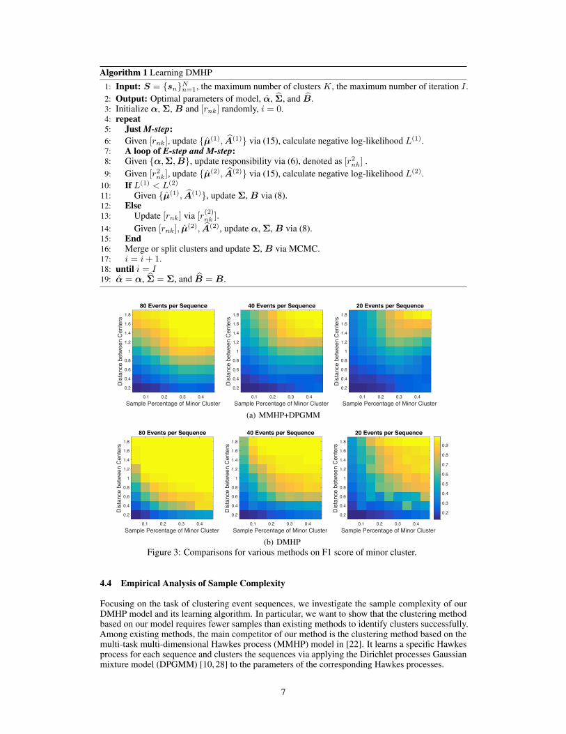
(b) DMHPFigure 3: Comparisons for various methods on F1 score of minor cluster.

4.4 Empirical Analysis of Sample Complexity

Focusing on the task of clustering event sequences, we investigate the sample complexity of ourDMHP model and its learning algorithm. In particular, we want to show that the clustering methodbased on our model requires fewer samples than existing methods to identify clusters successfully.Among existing methods, the main competitor of our method is the clustering method based on themulti-task multi-dimensional Hawkes process (MMHP) model in [22]. It learns a specific Hawkesprocess for each sequence and clusters the sequences via applying the Dirichlet processes Gaussianmixture model (DPGMM) [10, 28] to the parameters of the corresponding Hawkes processes.

7

Table 1: Clustering Purity on Synthetic Data.Sine-like φ(t) Piecewise constant φ(t)

C KVAR+ LS+ MMHP+ DMHP VAR+ LS+ MMHP+ DMHPDPGMM DPGMM DPGMM DPGMM DPGMM DPGMM

5

2 0.5235 0.5639 0.5917 0.9898 0.5222 0.5589 0.5913 0.80853 0.3860 0.5278 0.5565 0.9683 0.3618 0.4402 0.4517 0.77154 0.2894 0.4365 0.5112 0.9360 0.2901 0.3365 0.3876 0.70565 0.2543 0.3980 0.4656 0.9055 0.2476 0.2980 0.3245 0.6774

Following the work in [14], we demonstrate the superiority of our DMHP-based clustering methodthrough the comparison on the identifiability of minor clusters given finite number of samples.Specifically, we consider a binary clustering problem with 500 event sequences. For the k-th cluster,k = 1, 2, Nk event sequences are generated via a 1-dimensional Hawkes processes with parameterθk = µk,Ak. Taking the parameter as a representation of the clustering center, we can calculatethe distance between two clusters as d = ‖θ1 − θ2‖2. Assume that N1 < N2, we denote the firstcluster as “minor” cluster, whose sample percentage is π1 = N1

N1+N2. Applying our DMHP model

and its learning algorithm to the data generated with different d’s and π1’s, we can calculate the F1scores of the minor cluster w.r.t. d, π. The high F1 score means that the minor cluster is identifiedwith high accuracy. Fig. 3 visualizes the maps of F1 scores generated via different methods w.r.t. thenumber of events per sequence. We can find that the F1 score obtained via our DMHP-based methodis close to 1 in most situations. Its identifiable area (yellow part) is much larger than that of theMMHP+DPGMM method consistently w.r.t. the number of events per sequence. The unidentifiablecases happen only in the following two situations: the parameters of different clusters are nearlyequal (i.e., d→ 0); or the minor cluster is extremely small (i.e., π1 → 0). The enlarged version ofFig. 3 is given in the supplementary file.

5 Experiments

To demonstrate the feasibility and the efficiency of our DMHP-based sequence clustering method, wecompare it with the state-of-the-art methods, including the vector auto-regressive (VAR) method [12],the Least-Squares (LS) method in [7], and the multi-task multi-dimensional Hawkes process (MMHP)in [22]. All of the three competitors first learn features of sequences and then apply the DPGMM [10]to cluster sequences. The VAR discretizes asynchronous event sequences to time series and learnstransition matrices as features. Both the LS and the MMHP learn a specific Hawkes process for eachevent sequence. For each event sequence, we calculate its infectivity matrix Φ = [φcc′ ], where theelement φcc′ is the integration of impact function (i.e.,

∫∞0φcc′(t)dt), and use it as the feature.

For the synthetic data with clustering labels, we use clustering purity [24] to evaluate various methods:

Purity =1

N

∑K

k=1maxj∈1,...,K′ |Wk ∩ Cj |,

whereWk is the learned index set of sequences belonging to the k-th cluster, Cj is the real index setof sequence belonging to the j-th class, and N is the total number of sequences. For the real-worlddata, we visualize the infectivity matrix of each cluster and measure the clustering consistency viaa cross-validation method [39, 41]. The principle is simple: because random sampling does notchange the clustering structure of data, a clustering method with high consistency should preservethe pairwise relationships of samples in different trials. Specifically, we test each clustering methodwith J (= 100) trials. In the j-th trial, data is randomly divided into two folds. After learning thecorresponding model from the training fold, we apply the method to the testing fold. We enumerateall pairs of sequences within a same cluster in the j-th trial and count the pairs preserved in all othertrials. The clustering consistency is the minimum proportion of preserved pairs over all trials:

Consistency = minj∈1,..,J∑

j′ 6=j

∑(n,n′)∈Mj

1kj′n = kj′

n′(J − 1)|Mj |

,

whereMj = (n, n′)|kjn = kjn′ is the set of sequence pairs within same cluster in the j-th trial, andkjn is the index of cluster of the n-th sequence in the j-th trial.

8

1 2 3 4 5 6 7 8 9 100

10

20

30

40

50 DMHPMMHP

1 2 3 4 5 6 7 8 9 100

10

20

30

40DMHPMMHP

(a) Sine-like impact function

1 2 3 4 5 6 7 8 9 100

10

20

30

40

50 DMHPMMHP

1 2 3 4 5 6 7 8 9 100

10

20

30

40DMHPMMHP

(b) Piecewise constant impact functionFigure 4: The histograms of the number of clusters obtained via various methods on the two syntheticdata sets.

5.1 Synthetic Data

We generate two synthetic data sets with various clusters using sine-like impact functions andpiecewise constant impact functions respectively. In each data set, the number of clusters is set from 2to 5. Each cluster contains 400 event sequences, and each event sequence contains 50 (= Mn) eventsand 5 (= C) event types. The elements of exogenous base intensity are sampled uniformly from [0, 1].Each sine-like impact function in the k-th cluster is formulated as φkcc′ = bkcc′(1−cos(ωkcc′(t−skcc′))),where bkcc′ , ωkcc′ , skcc′ are sampled randomly from [π5 ,

2π5 ]. Each piecewise constant impact function

is the truncation of the corresponding sine-like impact function, i.e., 2bkcc′ × round(φkcc′/(2bkcc′)).

Table 1 shows the clustering purity of various methods on the synthetic data. Compared with thethree competitors, our DMHP obtains much better clustering purity consistently. The VAR simplytreats asynchronous event sequences as time series, which loses the information like the order ofevents and the time delay of adjacent events. Both the LS and the MMHP learn Hawkes process foreach individual sequence, which might suffer to over-fitting problem in the case having few eventsper sequence. These competitors decompose sequence clustering into two phases: learning featureand applying DPGMM, which is very sensitive to the quality of feature. The potential problemsabove lead to unsatisfying clustering results. Our DMHP method, however, is model-based, whichlearns clustering result directly and reduces the number of unknown variables greatly. As a result,our method avoids the problems of these three competitors and obtains superior clustering results.Additionally, the learning results of the synthetic data with piecewise constant impact functions provethat our DMHP method is relatively robust to the problem of model misspecification — althoughour Gaussian basis cannot fit piecewise constant impact functions well, our method still outperformsother methods greatly. Fig. 4 shows the histograms of the number of clusters obtained via variousmethods on our two synthetic data sets (K = 5). We can find that the distributions obtained by ourmethod are more concentrated to the real number of clusters.

5.2 Real-world Data

We test our clustering method on two real-world data sets. The first is the ICU patient flow data usedin [44], which is extracted from the MIMIC II data set [32]. This data set contains the transitionprocesses of 30, 308 patients among different kinds of care units. The patients can be clusteredaccording to their transition processes. The second is the IPTV data set in [20, 22], which contains7, 100 IPTV users’ viewing records collected via Shanghai Telecomm Inc. The TV programs arecategorized into 16 classes and the viewing behaviors more than 20 minutes are recorded. Similarly,the users can be clustered according to their viewing records. The event sequences in these two datahave strong but structural triggering patterns, which can be modeled via different Hawkes processes.

9

Table 2: Clustering Consistency on Real-world Data.Method VAR+DPGMM LS+DPGMM MMHP+DPGMM DMHP

ICU Patient 0.0901 0.1390 0.3313 0.3778IPTV User 0.0443 0.0389 0.1382 0.2004

5 10 15 20 250

20

40

60DMHPMMHP

(a) Histogram of K

Cluster 1

2 4 6 8 10

2

4

6

8

10

Cluster 2

2 4 6 8 10

2

4

6

8

10

Cluster 3

2 4 6 8 10

2

4

6

8

10

Cluster 4

2 4 6 8 10

2

4

6

8

10

Cluster 5

2 4 6 8 10

2

4

6

8

10

Cluster 6

2 4 6 8 10

2

4

6

8

10

Cluster 1

2 4 6 8 10

2

4

6

8

10

Cluster 2

2 4 6 8 10

2

4

6

8

10

Cluster 3

2 4 6 8 10

2

4

6

8

10

Cluster 4

2 4 6 8 10

2

4

6

8

10

Cluster 5

2 4 6 8 10

2

4

6

8

10

Cluster 6

2 4 6 8 10

2

4

6

8

10

Cluster 7

2 4 6 8 10

2

4

6

8

10

Cluster 8

2 4 6 8 10

2

4

6

8

10

Cluster 9

2 4 6 8 10

2

4

6

8

10

Cluster 10

2 4 6 8 10

2

4

6

8

10

Cluster 11

2 4 6 8 10

2

4

6

8

10

Cluster 12

2 4 6 8 10

2

4

6

8

10

Cluster 13

2 4 6 8 10

2

4

6

8

10

Cluster 14

2 4 6 8 10

2

4

6

8

10

Cluster 15

2 4 6 8 10

2

4

6

8

10

Cluster 16

2 4 6 8 10

2

4

6

8

10

Cluster 17

2 4 6 8 10

2

4

6

8

10

Cluster 18

2 4 6 8 10

2

4

6

8

10

Cluster 19

2 4 6 8 10

2

4

6

8

10

Cluster 20

2 4 6 8 10

2

4

6

8

10

(b) DMHP

Cluster 1

2 4 6 8 10

2

4

6

8

10

Cluster 2

2 4 6 8 10

2

4

6

8

10

Cluster 3

2 4 6 8 10

2

4

6

8

10

Cluster 4

2 4 6 8 10

2

4

6

8

10

Cluster 5

2 4 6 8 10

2

4

6

8

10

Cluster 6

2 4 6 8 10

2

4

6

8

10

Cluster 1

2 4 6 8 10

2

4

6

8

10

Cluster 2

2 4 6 8 10

2

4

6

8

10

Cluster 3

2 4 6 8 10

2

4

6

8

10

Cluster 4

2 4 6 8 10

2

4

6

8

10

Cluster 5

2 4 6 8 10

2

4

6

8

10

Cluster 6

2 4 6 8 10

2

4

6

8

10

Cluster 7

2 4 6 8 10

2

4

6

8

10

Cluster 8

2 4 6 8 10

2

4

6

8

10

Cluster 9

2 4 6 8 10

2

4

6

8

10

Cluster 10

2 4 6 8 10

2

4

6

8

10

Cluster 11

2 4 6 8 10

2

4

6

8

10

Cluster 12

2 4 6 8 10

2

4

6

8

10

Cluster 13

2 4 6 8 10

2

4

6

8

10

Cluster 14

2 4 6 8 10

2

4

6

8

10

Cluster 15

2 4 6 8 10

2

4

6

8

10

Cluster 16

2 4 6 8 10

2

4

6

8

10

Cluster 17

2 4 6 8 10

2

4

6

8

10

Cluster 18

2 4 6 8 10

2

4

6

8

10

Cluster 19

2 4 6 8 10

2

4

6

8

10

Cluster 20

2 4 6 8 10

2

4

6

8

10

(c) MMHP+DPGMMFigure 5: Comparisons on the ICU patient flow data.

Table 2 shows the performance of various clustering methods on the clustering consistency. We canfind that our method outperforms other methods obviously, which means that the clustering resultobtained via our method is more stable and consistent than other methods’ results. In Fig. 5 wevisualize the comparison for our method and its main competitor MMHP+DPGMM on the ICUpatient flow data. Fig. 5(a) shows the histograms of the number of clusters for the two methods. Wecan find that MMHP+DPGMM method tends to over-segment data into too many clusters. Our DMHPmethod, however, can find more compact clustering structure. The distribution of the number ofclusters concentrates to 6 and 19 for the two data sets, respectively. In our opinion, this phenomenonreflects the drawback of the feature-based method — the clustering performance is highly dependenton the quality of feature while the clustering structure is not considered sufficiently in the phase ofextracting feature. Taking learned infectivity matrices as representations of clusters, we compare ourDMHP method with MMHP+DPGMM in Figs. 5(b) and 5(c). The infectivity matrices obtained byour DMHP are sparse and with distinguishable structure, while those obtained by MMHP+DPGMMare chaotic — although MMHP also applies sparse regularizer to each event sequence’ infectivitymatrix, it cannot guarantee the average of the infectivity matrices in a cluster is still sparse. Samephenomena can also be observed in the experiments on the IPTV data. The clustering results of IPTVdata are shown in Fig. 6. Compared with the results obtained via MMHP+DPGMM, the histogramof the number of clusters obtained via our DMHP method is more concentrated and the infectivitymatrices of clusters are more structural and explainable.

6 Conclusion and Future Work

In this paper, we propose and discuss a Dirichlet mixture model of Hawkes processes and achievea model-based solution to event sequence clustering. We prove the identifiability of our modeland analyze the convergence, sample complexity and computational complexity of our learningalgorithm. In the aspect of methodology, we plan to study other potential priors, e.g., the prior basedon determinantial point processes (DPP) in [46], to improve the estimation of the number of clusters,and further accelerate our learning algorithm via optimizing inner iteration allocation strategy in nearfuture. Additionally, our model can be extended to Dirichlet process mixture model when K →∞.In that case, we plan to apply Bayesian nonparametrics to develop new learning algorithms.

7 Acknowledgment

This work is supported in part by NSF IIS-1639792, IIS-1717916, and CMMI-1745382.

10

15 20 25 300

10

20

30

40

50 DMHPMMHP

(a) Histogram of K

Cluster 1

5 10 15

5

10

15

Cluster 2

5 10 15

5

10

15

Cluster 3

5 10 15

5

10

15

Cluster 4

5 10 15

5

10

15

Cluster 5

5 10 15

5

10

15

Cluster 6

5 10 15

5

10

15

Cluster 7

5 10 15

5

10

15

Cluster 8

5 10 15

5

10

15

Cluster 9

5 10 15

5

10

15

Cluster 10

5 10 15

5

10

15

Cluster 11

5 10 15

5

10

15

Cluster 12

5 10 15

5

10

15

Cluster 13

5 10 15

5

10

15

Cluster 14

5 10 15

5

10

15

Cluster 15

5 10 15

5

10

15

Cluster 16

5 10 15

5

10

15

Cluster 17

5 10 15

5

10

15

Cluster 18

5 10 15

5

10

15

Cluster 1

5 10 15

5

10

15

Cluster 2

5 10 15

5

10

15

Cluster 3

5 10 15

5

10

15

Cluster 4

5 10 15

5

10

15

Cluster 5

5 10 15

5

10

15

Cluster 6

5 10 15

5

10

15

Cluster 7

5 10 15

5

10

15

Cluster 8

5 10 15

5

10

15

Cluster 9

5 10 15

5

10

15

Cluster 10

5 10 15

5

10

15

Cluster 11

5 10 15

5

10

15

Cluster 12

5 10 15

5

10

15

Cluster 13

5 10 15

5

10

15

Cluster 14

5 10 15

5

10

15

Cluster 15

5 10 15

5

10

15

Cluster 16

5 10 15

5

10

15

Cluster 17

5 10 15

5

10

15

Cluster 18

5 10 15

5

10

15

Cluster 19

5 10 15

5

10

15

Cluster 20

5 10 15

5

10

15

(b) DMHP

Cluster 1

5 10 15

5

10

15

Cluster 2

5 10 15

5

10

15

Cluster 3

5 10 15

5

10

15

Cluster 4

5 10 15

5

10

15

Cluster 5

5 10 15

5

10

15

Cluster 6

5 10 15

5

10

15

Cluster 7

5 10 15

5

10

15

Cluster 8

5 10 15

5

10

15

Cluster 9

5 10 15

5

10

15

Cluster 10

5 10 15

5

10

15

Cluster 11

5 10 15

5

10

15

Cluster 12

5 10 15

5

10

15

Cluster 13

5 10 15

5

10

15

Cluster 14

5 10 15

5

10

15

Cluster 15

5 10 15

5

10

15

Cluster 16

5 10 15

5

10

15

Cluster 17

5 10 15

5

10

15

Cluster 18

5 10 15

5

10

15

Cluster 1

5 10 15

5

10

15

Cluster 2

5 10 15

5

10

15

Cluster 3

5 10 15

5

10

15

Cluster 4

5 10 15

5

10

15

Cluster 5

5 10 15

5

10

15

Cluster 6

5 10 15

5

10

15

Cluster 7

5 10 15

5

10

15

Cluster 8

5 10 15

5

10

15

Cluster 9

5 10 15

5

10

15

Cluster 10

5 10 15

5

10

15

Cluster 11

5 10 15

5

10

15

Cluster 12

5 10 15

5

10

15

Cluster 13

5 10 15

5

10

15

Cluster 14

5 10 15

5

10

15

Cluster 15

5 10 15

5

10

15

Cluster 16

5 10 15

5

10

15

Cluster 17

5 10 15

5

10

15

Cluster 18

5 10 15

5

10

15

Cluster 19

5 10 15

5

10

15

Cluster 20

5 10 15

5

10

15

(c) MMHP+DPGMMFigure 6: Comparisons on the IPTV user data.

8 Supplementary File

8.1 The Proof of Local Identifiability

Before proving the local identifiability of our DMHP model, we first introduce some key concepts.A temporal point process is a random process whose realization consists of a list of discrete eventsin time ti with ti ∈ [0, T ]. Here [0, T ] is the time interval of the process. It can be equivalentlyrepresented as a counting process, N = N(t)|t ∈ [0, T ], where N(t) records the number ofevents before time t. A multi-dimensional point process with C types of event is represented byC counting processes NcCc=1 on a probability space (Ω,F,P). Nc = Nc(t)|t ∈ [0, T ], whereNc(t) is the number of type-c events occurring at or before time t. Ω = [0, T ] × C is the samplespace. C = 1, ..., C is the set of event types. F = (F(t))t∈R is the filtration representing the set ofevents sequence the process can realize until time t. P is the probability measure.

Hawkes process is a kind of temporal point processes having self-and mutually-triggering patterns.The triggering of historical events on current ones in a Hawkes process can be modeled as branchprocesses [8, 35]. As a result, Hawkes Process can be represented as a superposition of manynon-homogeneous Poisson process. Due to the superposition theorem of Poisson processes, thesuperposition of the individual processes is equivalent to the point process with summation oftheir intensity function. Given this we can break the counting process associated to each additionto the intensity function (or associated to each event): N(t) =

∑ni=0N

i(t), where N0(t) is thecounting process associated to the baseline intensity µ(t) and N i(t) is the non-homgenous Poissonprocess for the i-th branch. Similarly, we can write the intensity function of Hawkes process asλ(t) =

∑ni=0 λ

i(t), where λi(t) is the intensity of the i-th branch.

Definition 8.1. Two parameter points Θ1 and Θ2 are said to be observationally equivalent ifp(s; Θ1) = p(s; Θ2) for all samples s’s in sample space.Definition 8.2. A parameter point Θ0 is said to be locally identifiable if there exists an open neigh-borhood of Θ0 containing no other Θ in the parameter space which is observationally equivalent.Definition 8.3. Let I(Θ) be a matrix whose elements are continuous functions of Θ everywhere inthe parameter space. The point Θ0 is said to be a regular point of the matrix if there exists an openneighborhood of Θ0 in which I(Θ) has constant rank.

The information matrix I(Θ) is defined as

I(Θ) = Es[∂ log p(s; Θ)

∂Θ

∂ log p(s; Θ)

∂Θ>

]= Es

[1

p2(s; Θ)

∂p(s; Θ)

∂Θ

∂p(s; Θ)

∂Θ>

],

The local identifiability of our DMHP model is based on the following two theorems.Theorem 8.1. [26] The information matrix I(Θ) is positive definite if and only if there does notexist a nonzero vector of constants w such thatw> ∂p(s;Θ)

∂Θ = 0 for all samples s’s in sample space.

Theorem 8.2. [31] Let Θ0 be a regular point of the information matrix I(Θ). Then Θ0 is locallyidentifiable if and only if I(Θ0) is nonsingular.

11

To our DMHP model, the log-likelihood function is composed with differentiable functions of Θ.Therefore, the elements of information matrix I(Θ) are continuous functions w.r.t. Θ in the parameterspace. According to Theorems 8.1 and 8.2, our Theorem holds if and only if to each vector ∂p(s;Θ)

∂Θ

w.r.t. a point Θ, there does not exist a nonzero vector of constants w such that w> ∂p(s;Θ)∂Θ = 0 for

all event sequences s ∈ F.

Assume that there exists a nonzero w such that w> ∂p(s;Θ)∂Θ = 0 for all s ∈ F. We have the

following counter-evidence: Considering the simplest case — the mixture of two Poisson processes(or equivalently, two 1-dimensional Hawkes processes whose impact functions φ(t) ≡ 0), we canwrite its likelihood given a sequence with N events in [0, T ] as

p(sN ; Θ) = πλN1 exp(−Tλ1) + (1− π)λN2 exp(−Tλ2) = Λ1 + Λ2,

where Θ = [π, λ1, λ2]>, λ1 6= λ2. According to our assumption, we have

w>∂p(sN ; Θ)

∂Θ= w>

Λ1

π −Λ2

1−π( Nλ1− T )Λ1

( Nλ2− T )Λ2

= 0,

Denote the time stamp of the last event as tN , we can generate new event sequences sN+n∞n=1 viaadding n events in (tN , T ], and

w>∂p(sN+n; Θ)

∂Θ= w>

λn1Λ1

π − λn2

Λ2

1−π((N + n)− Tλ1)λn−1

1 Λ1

((N + n)− Tλ2)λn−12 Λ2

.w> ∂p(sN+n;Θ)

∂Θ = 0 for n = 0, ...,∞ requires w ≡ 0 or all ∂p(sN+n;Θ)∂Θ are coplanar. How-

ever, according to the formulation above, for arbitrary three different n1, n2, n3 ∈ 0, ...,∞,∑3i=1 αi

∂p(sN+ni;Θ)

∂Θ = 0 holds if and only if α1 = α2 = α3 = 0.3 Therefore, w ≡ 0, whichviolates the assumption above.

Such a counter-evidence can also be found in more general case, i.e., mixtures of multiple multi-dimensional Hawkes processes because Hawkes process is a superposition of many non-homogeneousPoisson process. As a result, according to Theorems 8.1 and 8.2, each point Θ in the parameterspace is regular point of I(Θ) and the I(Θ) is nonsingular, and thus, our DMHP model is locallyidentifiable.

8.2 The Selection of Basis Functions

In our work, we apply Gaussian basis functions to our model. We use the basis selection methodin [42] to decide the bandwidth and the number of basis functions. In particular, we focus onthe impact functions having Fourier transformation. The representation of impact function, i.e.,φcc′(t) =

∑Dd=1 acc′gd(t), can be explained as a sampling process, where adcc′Dd=1 can be viewed

as the discretized samples of φcc′(t) in [0, T ] and each gd(t) = κω(t, td) is sampling function withcut-off frequence ω and center td. Given training sequences S = sn = (ti, ci)Mn

i=1Nn=1, we canestimate λ(t) empirically via a Gaussian-based kernel density estimator:

λ(t) =∑N

n=1

∑Mn

i=1Gh(t− ti). (9)

HereGh(t−ti) = exp(− (t−ti)22h2 ) is a Gaussian kernel with the bandwidth h. Instead of computing (9),

we directly apply Silverman’s rule of thumb [34] to set optimal h = ( 4σ5

3∑nMn

)0.2, where σ is thestandard deviation of time stamps ti. Applying Fourier transform, we compute an upper bound for

3The derivation is simple. Interested reader can try the case with n1 = 0, n2 = 1, n3 = 3

12

the spectral of λ(t) as

|λ(ω)| =∣∣∣∣∫ ∞−∞

λ(t)e−jωtdt

∣∣∣∣ =

∣∣∣∣∑N

n=1

∑Mn

i=1

∫ ∞−∞

e−(t−ti)

2

2h2 e−jωtdt

∣∣∣∣≤∑N

n=1

∑Mn

i=1

∣∣∣∣∫ ∞−∞

e−(t−ti)

2

2h2 e−jωtdt

∣∣∣∣ =∑N

n=1

∑Mn

i=1

∣∣∣e−jωtie−ω2h2

2

√2πh2

∣∣∣≤∑N

n=1

∑Mn

i=1

∣∣e−jωti∣∣ ∣∣∣e−ω2h2

2

√2πh2

∣∣∣ =

(∑N

n=1Mn

√2πh2

)e−

ω2h2

2 .

(10)

Then, we can compute the upper bound of the absolute sum of the spectral higher than a certainthreshold ω0 as∫ ∞ω0

|λ(ω)|dω ≤(∑N

n=1Mn

√2πh2

)∫ ∞ω0

e−ω2h2

2 dω = π

(∑N

n=1Mn

)(1− 1√

2erf(ω0h)

),

where erf(x) = 1√π

∫ x−x e

−t2dt.

Therefore, give a bound of residual ε, we can find an ω0 guaranteeing∫∞ω0|λ(ω)|dω ≤ ε, or

erf(ω0h) ≥√

2 −√

2επ∑Nn=1Mn

. The proposed basis functions gd(t)Dd=1 are selected — each

gd(t) is a Gaussian function with cut-off frequency ω0 and center (d−1)TD , where D = dTω0

π e. Insummary, we propose Algorithm 2 to select basis functions.

Algorithm 2 Selecting basis functions1: Input: S = snNn=1, residual’s upper bound ε.2: Output: Basis functions gd(t)Dd=1.

3: Compute(∑N

n=1Mn

√2πh2

)e−

ω2h2

2 to bound |λ(ω)|.

4: Find the smallest ω0 satisfying∫∞ω0|λ(ω)|dω ≤ ε.

5: The Gaussian basis functions gd(t)Dd=1 are with cut-off frequency ω0 and centers (d−1)TD Dd=1,

where D = dTω0

π e.

8.3 Nested EM Framework

We consider a variational distribution having the following factorization:

q(Z,π,µ,A) = q(Z)q(π,µ,A) = q(Z)q(π)∏

kq(µk)q(Ak). (11)

An nested EM algorithm can be used to optimize (5).

Update Responsibility (E-step). In each outer iteration, the logarithm of the optimized factor q∗(Z)is approximated as

log q∗(Z)

=Eπ,µ,A[log p(S,Z,π,µ,A)] + C

=Eπ[log p(Z|π)] + Eµ,A[log p(S|Z,µ,A)] + C

=∑

n,kznk

(E[log πk] + E[log HP(sn|µk,Ak)]

)+ C

=∑

n,kznk

(E[log πk] + E[

∑ilog λkci(ti)−

∑c

∫ Tn

0

λkc (s)ds])

+ C

≈∑

n,kznk

(E[log πk] +

∑i

(logE[λkci(ti)]−


)−∑

cE[

∫ Tn

0

λkc (s)ds])

+C

=∑

n,kznk log ρnk + C.

(12)

13

where C is a constant, and each term E[log λkc (t)] is approximated via its second-order Taylor

expansion logE[λkc (t)]− Var[λkc (t)]2E2[λkc (t)]

[38]. Then, we have

log ρnk

=E[log πk] +∑i

(log(E[λkci(ti)])−


)−∑c

E[

∫ Tn

0

λkc (s)ds]

=E[log πk] +∑i

(log(E[µkci ] +

∑j<i,d

E[akcicjd]gd(τij))−Var[µkci ] +

∑j<i,d Var[akcicjd]g

2d(τij)

2(E[µkci ] +∑j<i,d E[akcicjd]gd(τij))

2

)−∑c

(TnE[µkc ] +∑i,d

E[akccid]Gd(Tn − ti))

=E[log πk] +∑i

(log(

√π

2βkci +

∑j<i,d

σkcicjdgd(τij))−4−π

2 (βkci)2 +

∑j<i,d(σ

kcicjd

gd(τij))2

2(√

π2β

kci +

∑j<i,d σ

kcicjd

gd(τij))2

)−∑c

(Tn

√π

2βkc +

∑i,d

σkccidGd(Tn − ti)),

where Gd(t) =∫ t

0gd(s)ds and τij = ti− tj . The second equation above is based on the prior that all

of the parameters are independent to each other. The term E[log πk] = ψ(αk)− ψ(∑k αk), where

ψ(·) is the digamma function.4 Then, the responsibility rnk is calculated as

rnk = E[znk] =ρnk∑j ρnj

, and Nk =∑

nrnk. (13)

It should be noted that here we increase q∗(Z) via maximizing its upper bound in each iterationbecause the difference between q∗(Z) and its upper bound is bounded tightly. In particular, q∗(Z)in (6) involves E[log λkci(ti)], which is approximated via Jensen’s inequality as logE[λkci(ti)]. Itactually is the first order Talyor expansion of E[log λkci(ti)]. The second order term is bounded welland the higher order terms can be ignored. We prove the rationality of our relaxation in the appendix.

Update Parameters (M-step). The optimal factor q∗(π,µ,A) is

log q∗(π,µ,A)

=∑k

log(p(µk)p(Ak)) + EZ [log p(Z|π)] + log p(π) +∑n,k

rnk log HP(sn|µk,Ak) + C. (14)

We can estimate the parameters of Hawkes processes via:

maxµ,A

log(p(µ)p(A)) +∑

n,krnk log HP(sn|µk,Ak).

Here, we need to use an iterative method to solve the above optimization problem. Specifically, weinitialize µ and A via the expectations of their distributions (used in E-step), i.e., µ =

√π2B and

A = Σ. Applying the Jensen’s inequality, we obtain the surrogate function of the objective function:

log(p(µ)p(A)) +∑n,k

rnk log HP(sn|µk,Ak)

=∑c,k

[logµkc −

1

2(µkcβkc

)2

]−∑

c,c′,d,k

akcc′dσkcc′d

+∑n,k

rnk

[∑i

log λkci(ti)−∑c

∫ Tn

0

λkc (s)ds

]

≥∑c,k

[logµkc −

1

2(µkcβkc

)2

]−∑

c,c′,d,k

akcc′dσkcc′d

+∑n,k

rnk

[∑i

(pkii log

µkcipii

+∑j<i,d

pkijd logakcicjdgd(τij)

pijd

)

−∑c

Tnµkc −

∑c,i,d

akccidGd(Tn − ti)]

= Q,

4Denote the gamma function as Γ(t) =∫∞0xt−1e−xdx, the digamma function is defined as ψ(t) =

ddt

ln Γ(t).

14

where pkii =µkci

λkci(ti)

, and pkijd =akcicjd

gd(τij)

λkci(ti)

. Setting ∂Q∂µkc

= 0 and ∂Q∂akcc′d

= 0, we have

µkc =−b+

√b2 − 4ac

2a, akcc′d =

∑n rnk

∑i:ci=c

∑j:cj=c′

pkijd

1/σkcc′d +∑n rnk

∑i:ci=c′

Gd(Tn − ti). (15)

where a = 1(βkc )2

, b =∑n rnkTn, c = −1−

∑n rnk

∑i:ci=c

pkii. After repeating several such inner

iterations, we can get optimal µ, A, and update distributions as

Σk = Ak, Bk =√

2/πµk. (16)

The distribution of clusters can be estimated via πk = NkN .

8.4 Update The Number of Clusters K via MCMC

In the case of infinite mixture model, we can apply the Markov chain Monte Carlo (MCMC) [11, 46,49] to update K via merging or splitting clusters.

Chose move type. We make a random choice to propose a combine or a split move. Let qm andqs = 1− qm denote the probability of proposing a merge and a split move, respectively, for a currentK. Following the work in [46], we use qm = 0.5 for K ≥ 2, and qm = 0 for K = 1.

Merge move. We randomly select a pair (k1, k2) of components to merge and form a new componentk. The probability of choosing (k1, k2) is qc(k1, k2) = 1

K(K−1) . For our model, we can apply thefollowing deterministic transformation to get new merged parameters:

πk = πk1 + πk2 , Ak =πk1

πkAk1 +

πk2

πkAk2 , µk =

πk1

πkµk1 +

πk2

πkµk2 . (17)

Then Σ andB are updated accordingly.

Split move. We randomly select a component k to split into two new components k1 and k2. Theprobability of choosing component k is qs(k) = 1

K . Different from the sampling method in previouswork [11, 46, 49], the splitting of parameters is an ill-posed problem with positive constraints. Here,we apply a simple heuristic transformation to get new splitting parameters:

πk1 = aπk, πk2 = (1− a)πk, a ∼ Be(1, 1),

Ak1 =1

2aAk, Ak2 =

1

2(1− a)Ak, µk1 =

1

2aµk, µk2 =

1

2(1− a)µk.

(18)

Then Σ andB are updated accordingly.

Acceptance. Given original parameters Θ and the new Θ′, we accept a merge/split move with theprobability min1, likelihood ratio× p(Θ′)

p(Θ) .

References[1] E. Bacry, K. Dayri, and J.-F. Muzy. Non-parametric kernel estimation for symmetric Hawkes

processes. application to high frequency financial data. The European Physical Journal B,85(5):1–12, 2012.

[2] D. M. Blei and M. I. Jordan. Variational inference for Dirichlet process mixtures. Bayesiananalysis, 1(1):121–143, 2006.

[3] C. Blundell, J. Beck, and K. A. Heller. Modelling reciprocating relationships with Hawkesprocesses. In NIPS, 2012.

[4] D. J. Daley and D. Vere-Jones. An introduction to the theory of point processes: volume II:general theory and structure, volume 2. Springer Science & Business Media, 2007.

[5] N. Du, M. Farajtabar, A. Ahmed, A. J. Smola, and L. Song. Dirichlet-Hawkes processes withapplications to clustering continuous-time document streams. In KDD, 2015.

[6] N. Du, L. Song, M. Yuan, and A. J. Smola. Learning networks of heterogeneous influence. InNIPS, 2012.

[7] M. Eichler, R. Dahlhaus, and J. Dueck. Graphical modeling for multivariate Hawkes processeswith nonparametric link functions. Journal of Time Series Analysis, 2016.

15

[8] M. Farajtabar, N. Du, M. Gomez-Rodriguez, I. Valera, H. Zha, and L. Song. Shaping socialactivity by incentivizing users. In NIPS, 2014.

[9] G. H. Golub, Z. Zhang, and H. Zha. Large sparse symmetric eigenvalue problems withhomogeneous linear constraints: the Lanczos process with inner–outer iterations. LinearAlgebra And Its Applications, 309(1):289–306, 2000.

[10] D. Görür and C. E. Rasmussen. Dirichlet process Gaussian mixture models: Choice of the basedistribution. Journal of Computer Science and Technology, 25(4):653–664, 2010.

[11] P. J. Green. Reversible jump Markov chain Monte Carlo computation and Bayesian modeldetermination. Biometrika, pages 711–732, 1995.

[12] F. Han and H. Liu. Transition matrix estimation in high dimensional time series. In ICML,2013.

[13] A. G. Hawkes. Spectra of some self-exciting and mutually exciting point processes. Biometrika,58(1):83–90, 1971.

[14] D. Kim. Mixture inference at the edge of identifiability. Ph.D. Thesis, 2008.[15] R. Lemonnier and N. Vayatis. Nonparametric Markovian learning of triggering kernels for

mutually exciting and mutually inhibiting multivariate Hawkes processes. In Machine Learningand Knowledge Discovery in Databases, pages 161–176. 2014.

[16] E. Lewis and G. Mohler. A nonparametric EM algorithm for multiscale Hawkes processes.Journal of Nonparametric Statistics, 2011.

[17] L. Li and H. Zha. Dyadic event attribution in social networks with mixtures of Hawkes processes.In CIKM, 2013.

[18] W. Lian, R. Henao, V. Rao, J. Lucas, and L. Carin. A multitask point process predictive model.In ICML, 2015.

[19] T. W. Liao. Clustering of time series data: a survey. Pattern recognition, 38(11):1857–1874,2005.

[20] D. Luo, H. Xu, H. Zha, J. Du, R. Xie, X. Yang, and W. Zhang. You are what you watch andwhen you watch: Inferring household structures from IPTV viewing data. IEEE Transactionson Broadcasting, 60(1):61–72, 2014.

[21] D. Luo, H. Xu, Y. Zhen, B. Dilkina, H. Zha, X. Yang, and W. Zhang. Learning mixturesof Markov chains from aggregate data with structural constraints. IEEE Transactions onKnowledge and Data Engineering, 28(6):1518–1531, 2016.

[22] D. Luo, H. Xu, Y. Zhen, X. Ning, H. Zha, X. Yang, and W. Zhang. Multi-task multi-dimensionalHawkes processes for modeling event sequences. In IJCAI, 2015.

[23] E. A. Maharaj. Cluster of time series. Journal of Classification, 17(2):297–314, 2000.[24] C. D. Manning, P. Raghavan, H. Schütze, et al. Introduction to information retrieval, volume 1.

Cambridge university press Cambridge, 2008.[25] C. Maugis, G. Celeux, and M.-L. Martin-Magniette. Variable selection for clustering with

Gaussian mixture models. Biometrics, 65(3):701–709, 2009.[26] E. Meijer and J. Y. Ypma. A simple identification proof for a mixture of two univariate normal

distributions. Journal of Classification, 25(1):113–123, 2008.[27] B. A. Ogunnaike and W. H. Ray. Process dynamics, modeling, and control. Oxford University

Press, USA, 1994.[28] C. E. Rasmussen. The infinite Gaussian mixture model. In NIPS, 1999.[29] J. G. Rasmussen. Bayesian inference for Hawkes processes. Methodology and Computing in

Applied Probability, 15(3):623–642, 2013.[30] P. Reynaud-Bouret, S. Schbath, et al. Adaptive estimation for Hawkes processes; application to

genome analysis. The Annals of Statistics, 38(5):2781–2822, 2010.[31] T. J. Rothenberg. Identification in parametric models. Econometrica: Journal of the Econometric

Society, pages 577–591, 1971.[32] M. Saeed, C. Lieu, G. Raber, and R. G. Mark. MIMIC II: a massive temporal ICU patient

database to support research in intelligent patient monitoring. In Computers in Cardiology,2002, pages 641–644. IEEE, 2002.

[33] B. Shahriari, K. Swersky, Z. Wang, R. P. Adams, and N. de Freitas. Taking the human out ofthe loop: A review of Bayesian optimization. Proceedings of the IEEE, 104(1):148–175, 2016.

[34] B. W. Silverman. Density estimation for statistics and data analysis, volume 26. CRC press,1986.

[35] A. Simma and M. I. Jordan. Modeling events with cascades of Poisson processes. In UAI, 2010.

16

[36] J. Snoek, H. Larochelle, and R. P. Adams. Practical Bayesian optimization of machine learningalgorithms. In NIPS, 2012.

[37] R. Socher, A. L. Maas, and C. D. Manning. Spectral Chinese restaurant processes: Nonpara-metric clustering based on similarities. In AISTATS, 2011.

[38] Y. W. Teh, D. Newman, and M. Welling. A collapsed variational Bayesian inference algorithmfor latent Dirichlet allocation. In NIPS, 2006.

[39] R. Tibshirani and G. Walther. Cluster validation by prediction strength. Journal of Computa-tional and Graphical Statistics, 14(3):511–528, 2005.

[40] J. J. Van Wijk and E. R. Van Selow. Cluster and calendar based visualization of time series data.In IEEE Symposium on Information Visualization, 1999.

[41] U. Von Luxburg. Clustering Stability. Now Publishers Inc, 2010.[42] H. Xu, M. Farajtabar, and H. Zha. Learning Granger causality for Hawkes processes. In ICML,

2016.[43] H. Xu, D. Luo, and H. Zha. Learning Hawkes processes from short doubly-censored event

sequences. In ICML, 2017.[44] H. Xu, W. Wu, S. Nemati, and H. Zha. Patient flow prediction via discriminative learning

of mutually-correcting processes. IEEE Transactions on Knowledge and Data Engineering,29(1):157–171, 2017.

[45] H. Xu, Y. Zhen, and H. Zha. Trailer generation via a point process-based visual attractivenessmodel. In IJCAI, 2015.

[46] Y. Xu, P. Müller, and D. Telesca. Bayesian inference for latent biologic structure with determi-nantal point processes (DPP). Biometrics, 2016.

[47] S. J. Yakowitz and J. D. Spragins. On the identifiability of finite mixtures. The Annals ofMathematical Statistics, pages 209–214, 1968.

[48] S.-H. Yang and H. Zha. Mixture of mutually exciting processes for viral diffusion. In ICML,2013.

[49] Z. Zhang, K. L. Chan, Y. Wu, and C. Chen. Learning a multivariate Gaussian mixture modelwith the reversible jump MCMC algorithm. Statistics and Computing, 14(4):343–355, 2004.

[50] Q. Zhao, M. A. Erdogdu, H. Y. He, A. Rajaraman, and J. Leskovec. SEISMIC: A self-excitingpoint process model for predicting tweet popularity. In KDD, 2015.

[51] K. Zhou, H. Zha, and L. Song. Learning social infectivity in sparse low-rank networks usingmulti-dimensional Hawkes processes. In AISTATS, 2013.

[52] K. Zhou, H. Zha, and L. Song. Learning triggering kernels for multi-dimensional Hawkesprocesses. In ICML, 2013.

17

abstract of ece georgia institute of technology [email protected] hongyuan zha college of...

Documents