abstract of my phd dissertation
TRANSCRIPT

Nonparametric Density Estimation Methods withApplication to the U.S. Crop Insurance Program
by
Zongyuan Shang
A Thesispresented to
The University of Guelph
In partial fulfilment of requirementsfor the degree of
Doctor of Philosophyin
Food, Agricultural and Resource Economics
Guelph, Ontario, Canada
c©Zongyuan Shang, May, 2015

ABSTRACT
NONPARAMETRIC DENSITY ESTIMATION METHODS WITHAPPLICATION TO THE U.S. CROP INSURANCE PROGRAM
Zongyuan ShangUniversity of Guelph, 2015
Advisor:Professor Alan P. Ker
Theoretically, the bias reduction and the variance reduction nonparametric density
estimators could have but not yet been combined. Practically, accurate estimation of
premiums is a necessary condition for the financial solvency of the U.S. crop insurance
program as well as to mitigate, to the extent possible, problems of moral hazard and
adverse selection. Typically, premiums are derived from crop yield density which
is parametrically or nonparametrically estimated by historical data. Unfortunately,
valid historical yield data is limited.
To meet these challenges, I develop two novel nonparametric density estimators
denoted as Comb1 and Comb2 which selectively borrow information from extraneous
sources. They have the advantage to reduce not only the estimation bias but also
variance. By combining bias reduction and variance reduction estimators in different
ways, Comb1 unifies the standard kernel estimator, Jones’ bias reduction estimator
and Ker’s possibly similar estimator while Comb2 unifies the standard kernel esti-
mator, Ker’s possibly similar estimator, and different from Comb1, the conditional
estimator.
Numerical simulations suggest the two proposed estimators outperform a number
of existing methods: if the true densities are known, Comb1 and Comb2 are far
ahead with no obvious peers; if the true densities are assumed to be unknown and
bandwidths are selected by maximum likelihood cross-validation, Comb1 and Comb2
still have promising performance, especially Comb2.

Finally, the two estimators are applied to rate crop insurance contracts over the
alternatives in out-of-sample simulation games. Statistically and economically signifi-
cant improvements are found. Given the size of the crop insurance program, updating
the government’s density estimation method to Comb1 or Comb2 may potentially
save enormous amount of taxpayers’ money. Sensitivity analysis where only data of
the most recent 25 or 15 years is used suggests the findings are robust to missing
historical yield data, implying that by adopting Comb1 or Comb2 the Supplemen-
tal Coverage Option, a new crop insurance option that provides additional coverage
to farmer, could potentially be expanded to crops and areas with significantly less
historical data.

iv
ACKNOWLEDGMENTS
Foremost, thank you to my advisor Dr. Alan Ker for your insightful guidance, encour-
agement and timely help. Your vision, leadership and support enabled the completion
of this thesis and tremendously helped me to grow intellectually, to question and to
reason. To my advisory committee members Dr. John Cranfield, Dr. Getu Hailu and
Dr. Ze’ev Gedalof, thank you for your support and insightful feedback. To my exam-
ination committee chair Dr. Alfons Weersink, internal examiner Dr. Brady Deaton
and external examiner Dr. J. Roy Black, I really appreciate your time and valuable
comments. Thank you to the FARE family, the faculty, staff and students, especially
Kathryn, Pat and Debbie, I really appreciate the welcoming atmosphere.
Thank you to my FAREes friends, especially Peter, Tor, Cheryl and Johanna for
the enjoyable memories and unforgettable friendship. I cherish them dearly. Thank
you Na and Liyan, Juliette, Zhige, Li, Qianru and Heying, I’m very grateful for your
friendship, help and support. To my friends back home in China, thank you for your
continuous support. The financial support from China Scholarship Council (CSC) is
greatly appreciated.
To my family, I love you all and really appreciate everything you did for me.
To Sihui, you are the love of my life and I am indebted for your love, patience and
support.
Thank you God.
v
Contents
1 Introduction 1
1.1 Insurance in U.S. Agriculture . . . . . . . . . . . . . . . . . . . . . . 1
1.2 Motivation Purpose and Objective . . . . . . . . . . . . . . . . . . . . 2
1.2.1 Motivation . . . . . . . . . . . . . . . . . . . . . . . . . . . . . 2
1.2.2 Purpose . . . . . . . . . . . . . . . . . . . . . . . . . . . . . . 5
1.2.3 Objectives . . . . . . . . . . . . . . . . . . . . . . . . . . . . . 5
1.3 Organization of the Thesis . . . . . . . . . . . . . . . . . . . . . . . . 5
1.4 Contributions of the Thesis . . . . . . . . . . . . . . . . . . . . . . . 6
2 Literature Review 7
2.1 Parametric Approach . . . . . . . . . . . . . . . . . . . . . . . . . . . 7
2.2 Semiparametric Approach . . . . . . . . . . . . . . . . . . . . . . . . 8
2.3 Nonparametric Approach . . . . . . . . . . . . . . . . . . . . . . . . . 9
2.3.1 Standard Kernel Density Estimator . . . . . . . . . . . . . . . 11
2.3.2 Empirical Bayes Nonparametric Kernel Density Estimator . . 18
2.3.3 Conditional Density Estimator . . . . . . . . . . . . . . . . . . 20
2.3.4 Jones Bias Reduction Estimator . . . . . . . . . . . . . . . . . 22
2.3.5 Possibly Similar Estimator . . . . . . . . . . . . . . . . . . . . 23
2.4 Summary . . . . . . . . . . . . . . . . . . . . . . . . . . . . . . . . . 24
3 Proposed Estimators 26
3.1 Comb1 . . . . . . . . . . . . . . . . . . . . . . . . . . . . . . . . . . . 29

vi
3.2 Comb2 . . . . . . . . . . . . . . . . . . . . . . . . . . . . . . . . . . . 31
3.3 Proofs . . . . . . . . . . . . . . . . . . . . . . . . . . . . . . . . . . . 33
3.4 Summary . . . . . . . . . . . . . . . . . . . . . . . . . . . . . . . . . 38
4 Simulation 40
4.1 Some Considerations . . . . . . . . . . . . . . . . . . . . . . . . . . . 41
4.2 True Densities Are Known . . . . . . . . . . . . . . . . . . . . . . . . 44
4.2.1 Low Similarity . . . . . . . . . . . . . . . . . . . . . . . . . . 44
4.2.2 Moderate Similarity . . . . . . . . . . . . . . . . . . . . . . . 46
4.2.3 Identical . . . . . . . . . . . . . . . . . . . . . . . . . . . . . . 52
4.3 True Densities Are Unknown . . . . . . . . . . . . . . . . . . . . . . . 53
4.3.1 Low Similarity . . . . . . . . . . . . . . . . . . . . . . . . . . 55
4.3.2 Moderate Similarity . . . . . . . . . . . . . . . . . . . . . . . 57
4.3.3 Identical . . . . . . . . . . . . . . . . . . . . . . . . . . . . . . 59
4.4 Summary . . . . . . . . . . . . . . . . . . . . . . . . . . . . . . . . . 60
5 Application 62
5.1 Data . . . . . . . . . . . . . . . . . . . . . . . . . . . . . . . . . . . . 62
5.2 Empirical Considerations . . . . . . . . . . . . . . . . . . . . . . . . . 65
5.3 Design of the Game . . . . . . . . . . . . . . . . . . . . . . . . . . . . 75
5.4 Results . . . . . . . . . . . . . . . . . . . . . . . . . . . . . . . . . . . 78
5.5 Sensitivity Analysis . . . . . . . . . . . . . . . . . . . . . . . . . . . . 81
5.6 Summary . . . . . . . . . . . . . . . . . . . . . . . . . . . . . . . . . 83
6 Conclusions and Future Research 87
6.1 Conclusions . . . . . . . . . . . . . . . . . . . . . . . . . . . . . . . . 87
6.2 Future Research . . . . . . . . . . . . . . . . . . . . . . . . . . . . . . 91
Bibliography 93

vii
Appendices 97
A: Pseudo Game Results When Insurance Company Uses Cond . . . . . . 98
B: Weight λ in Conditional Estimator . . . . . . . . . . . . . . . . . . . . . 99
C: R code — True Densities Are Known and Bandwidth Selected by Mini-
mizing ISE . . . . . . . . . . . . . . . . . . . . . . . . . . . . . . . . . 101
D: R code — True Densities Are Unknown and Bandwidth Selected by
Cross-validation . . . . . . . . . . . . . . . . . . . . . . . . . . . . . . 111
E: R code — Raw Yield Data to Adjusted Yield Data . . . . . . . . . . . . 118
F: R code — Empirical Game . . . . . . . . . . . . . . . . . . . . . . . . . 123
G: R code — Sensitivity Analysis . . . . . . . . . . . . . . . . . . . . . . . 136

viii
List of Figures
2.1 Illustration of standard kernel density estimation . . . . . . . . . . . 12
2.2 Changing data and the corresponding estimated density . . . . . . . . 13
2.3 Changing bandwidth and the corresponding estimated density . . . . 16
3.1 Combining bias and variance reduction method to form Comb1 and
Comb2 . . . . . . . . . . . . . . . . . . . . . . . . . . . . . . . . . . . 28
3.2 The relationship between the estimators . . . . . . . . . . . . . . . . 33
4.1 Integrated squared error illustration . . . . . . . . . . . . . . . . . . . 41
4.3 The five moderately similar densities . . . . . . . . . . . . . . . . . . 48
5.1 County-level average corn yield for four randomly sampled counties,
Illinois . . . . . . . . . . . . . . . . . . . . . . . . . . . . . . . . . . . 63
5.2 Crop reporting districts in Illinois . . . . . . . . . . . . . . . . . . . . 64
5.3 The estimated two-knot spline trend in representative counties . . . . 69
5.4 Detrend and hetroscedasticity corrected yield . . . . . . . . . . . . . 71
5.5 Estimated corn yiled densities in Henry, Illinois with 1955-2009 data . 72
5.6 Estimated densities from different methods (1/2) . . . . . . . . . . . 73
5.7 Estimated densities from different methods (2/2) . . . . . . . . . . . 74
5.8 The decision rule of private insurance company . . . . . . . . . . . . 76

ix
List of Tables
4.1 The Nine Dissimilar Densities in Marron and Wand (1992) . . . . . . 44
4.2 MISE×1000 for Dissimilar True Densities, Bandwidths from Minimiz-
ing MISE . . . . . . . . . . . . . . . . . . . . . . . . . . . . . . . . . 47
4.3 Five Moderately Similar Densities in Ker and Ergün (2005) . . . . . 49
4.4 MISE×1000 for Moderately Similar True Densities, Bandwidths from
Minimizing MISE . . . . . . . . . . . . . . . . . . . . . . . . . . . . . 50
4.5 MISE×1000 for Identical True Density, Bandwidths from Minimizing
MISE . . . . . . . . . . . . . . . . . . . . . . . . . . . . . . . . . . . 52
4.6 MISE×1000 for Dissimilar True Densities, Bandwidths from Cross-
Validation . . . . . . . . . . . . . . . . . . . . . . . . . . . . . . . . . 56
4.7 MISE×1000 for Moderately Similar True Densities, Bandwidths from
Cross-Validation . . . . . . . . . . . . . . . . . . . . . . . . . . . . . . 58
4.8 MISE×1000 for Identical True Density, Bandwidths from Cross-Validation 59
5.1 Summary Statistics of Yield Data, Corn, Illinois, 1955-2013 . . . . . . 64
5.2 Out-of-sample Contracts Rating Game Results: Corn, Illinois . . . . . 79
5.3 Out-of-sample Contracts Rating Game Results: Soybean, Illinois . . . 80
5.4 Out-of-sample Contracts Rating Game Results: Sensitivity to Data
Length, Corn, IL . . . . . . . . . . . . . . . . . . . . . . . . . . . . . 85
5.5 Out-of-sample Contracts Rating Game Results: Sensitivity to Data
Length, Soybean, IL . . . . . . . . . . . . . . . . . . . . . . . . . . . 86

x
1 Out-of-sample Contracts Rating Game Results: Insurance Company
Using Cond, Corn, Illinois . . . . . . . . . . . . . . . . . . . . . . . . 98
2 Out-of-sample Contracts Rating Game Results: Insurance Company
Using Cond, Soybean, Illinois . . . . . . . . . . . . . . . . . . . . . . 98

Chapter 1
Introduction
1.1 Insurance in U.S. Agriculture
The 2014 farm bill has shifted monies from traditional farm price and income support
to risk management, solidifying crop insurance as the primary tool for farmers to
deal with production and price risk. In 2014, total government liabilities associated
with the crop insurance program exceeded $108.5 billion. The size of the program
is unprecedented and is likely to grow. According to an April 2014 Congressional
Budget Office estimate, for fiscal years 2014 through 2023, crop insurance program
costs are expected to average $8.9 billion annually.
Among those costs, a large share goes to premium subsidy. The United States
Department of Agriculture’s Risk Management Agency (RMA), the agency that ad-
ministers the crop insurance program, stated that subsidies for crop insurance pre-
miums accounted for $42.1 billion, or about 72%, of the $58.7 billion total program
costs from 2003 through 2012. More U.S. farmlands are covered by crop insurance as
the government increases its subsidy on crop insurance premium. As of 2013, 295.8
million acres of farmlands have been insured, which is 89% of eligible acres. The total
premium in this year was 11.8 billion. Farmers paid 4.5 billion of it. The rest, a large
share of 62% (7.3 billion) is payed by government subsidy.
1

1.2 Motivation Purpose and Objectives
1.2.1 Motivation
There are both empirical and theoretical gaps which motivate this research. They
are discussed in the following two subsections.
Empirical Motivation: The Challenge of Crop Insurance in U.S.
As introduced in the previous section, the monies directed toward crop insurance are
unprecedented and are likely to grow under the 2014 farm bill. However, the U.S.
crop insurance program faces two challenges: (i) insufficient historical yield data, and
(ii) the problem of asymmetric information. Challenge (i) is that there is at best 50
years of historical yield data to estimate low probability events. Moreover, given the
technological advances in seed development, the usefulness of the earlier yield data
(1950-70s) in estimating current losses is questionable. This challenges nonparametric
density estimation methods because they usually require large sample size for a sound
estimation. Interestingly, there are normally a large number of counties in a state each
with possibly similar underlying yield data-generating processes. One may possibly
improve the estimation efficiency by utilizing data from other counties. This is of
particular policy interest. In the U.S. crop insurance program, the government sets
the premium rates for insurance policies through RMA. As noted by Ker (2014), the
current RMA method does not explicitly use information from extraneous counties.
By incorporating such information, one might improve the current method. To be
more specific, if the true densities of all counties are identical, all yield data should be
pooled together to estimate a single density for all counties (i.e., “borrow” everything).
If the true densities of the extraneous counties are similar to the density of the county
of interest, some information (such as the shape of the densities in other counties)
2

should be “borrowed”. If the true densities are very dissimilar, only data from the
own county should be used (i.e., “borrow” nothing). Logically, such a flexible density
estimation method should be more efficient than the one currently adopted by RMA.
As for challenge (ii), the agriculture insurance markets, similar to other insur-
ance markets, also face problems of asymmetric information. That is the problem of
adverse selection (Stiglitz, 1975; Akerlof, 1970) before the purchase of an insurance
policy and moral hazard (Spence, 1977) after the purchase of an insurance policy.
Take crop insurance as an example. Moral hazard is found where insured farmers
perform riskier farming practices after buying the insurance. Evidences of moral haz-
ard are documented in the literature. Such as neglecting proper crop care (Horowitz
and Lichtenberg, 1993), purposely not using fertilizers (Babcock and Hennessy, 1996)
and sometimes even intentionally aiming for crop failure in order to collect indemnity
(Chambers, 1989; Smith and Goodwin, 1996). More evidence can be found in Smith
and Goodwin (1996) and Knight and Coble (1999).
The problem of moral hazard is mitigated in area-yield based group insurance
products (such as GRP, GRIP). After buying such products, an individual farmer
is less likely to take riskier farming practices. The reason is that whatever he does
will not affect his own gain. Indemnity is triggered by the average yield in the
area. As each farm is only a small proportion, an individual farmer’s riskier action
is not likely to influence the average yield in the whole area. This research focuses
on area-yield based group insurance products and moral hazard is not a concern.
Adverse selection, where farmers with relatively higher risk buy more insurance while
low-risk farmers reduce their coverage, is indeed a problem. Having more private
information, insurance contract policyholders (farmers) have a better understanding
of the risks they face, which helps them to identify whether they are in a high-risk or
low-risk category. As more and more high-risk farmers self-select to buy insurance,
the insurance company will no longer be able to cover the indemnity by the collected
3

premium. Ultimately, as a typical story of the market for lemons, the insurance
companies will run out of business and the market fails.
More accurately calculated premium rates can help to mitigate, to the extent
possible, problems of adverse selection. To calculate premium rates, accurate esti-
mation of conditional yield density is key (Ker and Goodwin, 2000). This point can
be better understood by examining how the actuarially fair premium is calculated.
Define y as the random variable of average yield in an area, λye as the guaranteed
yield where 0≤ λ≤ 1 is the coverage level and ye is the predicted yield, fy(y|It) is the
density function of the yield conditional on information available at time t. An actu-
arially fair premium, π, is equal to the expected indemnity as shown in the following
equation:
π = P (y < λye)(λye−E(y|y < λye)) =∫ λye
0(λye−y)fy(y|It)dy. (1.1)
Different conditional yield density fy(y|It) will result in different premium. To cor-
rectly calculate the actuarially fair premium, it is necessary to estimate the conditional
yield density with precision.
Theoretical Motivation: A More Generalized Nonparametric Density Es-
timator
In the literature, density estimation methods can be grouped into three categories:
parametric, semiparametric and nonparametric. In the nonparametric category, a
number of interesting density estimators have been proposed to estimate yield density.
Of focus here are the bias reduction estimator by Jones, Linton, and Nielsen (1995),
the conditional estimator by Hall, Racine, and Li (2004) and the possibly similar
estimator by Ker (2014). However, these methods are isolated, leaving substantial
efficiency gain uncaptured were they combined. Theoretically, a more generalized
4

estimator which unifies these (or at least some of these) estimators into one would
be more efficient. At least, the generalized estimator will be as good as each single
estimator; each single estimator is just a spacial case of the generalized estimator.
However, this has not been done yet. This research attempts to fill such a theoretical
gap.
1.2.2 Purpose
The purpose of this study is to propose new nonparametric density estimation meth-
ods which could improve density estimation accuracy. The new estimators would
unify several existing density estimators and reduce loss ratio when applied to rating
crop insurance contracts.
1.2.3 Objectives
There are several main objectives of this study: (a) to propose new density estimators;
(b) to evaluate the performance of the new estimators when the true densities are
known; (c) to evaluate the performance of the new estimators when the true densities
are unknown; and (d) to apply the new estimators in rating crop insurance contracts
and test the stability of the estimators when sample size is reduced.
1.3 Organization of the Thesis
This thesis is organized into six chapters. The U.S. agriculture insurance market, the
research motivation and purpose, objectives and contributions have been presented in
Chapter 1. Chapter 2 is the literature review of three categories of density estimation
methods: parametric, semiparametric and nonparametric. The two new proposed
estimators, Comb1 and Comb2, are presented in Chapter 3. Chapter 4 evaluates
the performance of the two proposed estimators when the smoothing parameters
5

are selected by different methods. Chapter 5 contains an application where the two
proposed methods are applied to rate crop insurance policies. Finally, Chapter 6
presents the main conclusions.
1.4 Contributions of the Thesis
This thesis contributes to the broader literature on nonparametric density estima-
tion in econometrics and insurance policy rating in agricultural economics. There
are several unique density estimators1 each with its own merits in the literature.
Such as Jones, Linton, and Nielsen (1995) and Ker (2014) which reduce estimation
bias and Hall, Racine, and Li (2004) which reduces estimation variance. However,
they are isolated, leaving substantial efficiency gain uncaptured were they combined.
This thesis presents two novel estimators, Comb1 and Comb2, to fill such a gap.
In different ways, each of them combines several previous estimators into one unified
form. More specifically, Comb1 is a generalized estimator which contains the standard
kernel density estimator, Jones’ bias reduction density estimator and Ker’s possibly
similar density estimator as special cases. And Comb2 encapsulates the standard
kernel density estimator, Ker’s possibly similar density estimator and the conditional
density estimator into another generalized estimator. Both numerical simulation and
empirical application to U.S. crop insurance program demonstrate that the two pro-
posed estimators yield non-trivial efficiency improvement, outperforming a number of
existing alternative methods. Empirically, the two proposed estimators outperform a
number of their peers as well as the RMA’s current rating method. By adopting the
two proposed density estimators, the private insurance company is able to adversely
select against the government and retain contracts with significantly lower loss ratio.
1The standard kernel estimator (reviewed in section 2.3.1), the Jones’ bias reduction method(reviewed in section 2.3.4), the conditional density estimator (reviewed in 2.3.3) and Ker’s possiblysimilar estimator (reviewed in section 2.3.5).
6

Chapter 2
Literature Review
Generally, the density estimation methods are divided into three categories: paramet-
ric, semiparametric and nonparametric. I briefly review them in the following three
sections.
2.1 Parametric Approach
A significant number of parametric methods have been proposed to estimate yield
densities. Most of them concentrate on determining the appropriate parametric fam-
ily that best characterizes the true data-generating process. The commonly used
distributions include Normal, Beta, and Weibull.
Many researches assumed county-level crop yields follow a normal distribution
(Botts and Boles, 1958; Just andWeninger, 1999; Ozaki, Goodwin, and Shirota, 2008).
However, one can not directly apply central limit theorem and conclude that the
average yields follow a normal distribution. The reason is that the yields data within
a county are spatially correlated (Goodwin and Ker, 2002). In addition, evidence
against normality, such as negative skewness, were later found (Day, 1965; Taylor,
1990; Ramírez, 1997; Ramirez, Misra, and Field, 2003). More recently, Du et al.
(2012) found exogenous geographic and climate factors, such as better soils, less
overheating damage, more growing season precipitation and irrigation, make crop
yield distributions more negatively skewed.
Despite the prevailing consensus on non-normality, Just and Weninger (1999)
strongly defended that crop yields are normally distributed. They argued that rejection
7

of normality may have been caused by data limitations. Therefore, normality cannot
be rejected at least for some yield data and should be reconsidered. Tolhurst and Ker
(2015) used a mixture normal approach. The Beta distribution, with more flexible
shapes, was considered in the literature as an alternative of normal distribution (e.g.
Day, 1965; Nelson and Preckel, 1989; Tirupattur, Hauser, and Chaherli, 1996; Ozaki,
Goodwin, and Shirota, 2008). The Weibull distribution was also explored in the lit-
erature. It can be asymmetric with a flexible wide range of skewness and kurtosis
and is bounded below by zero. These features make the Weibull suitable for modeling
yield distribution. Sherrick et al. (2004) found that Beta and Weibull distributions
were the best fit for both corn and soybean yields, while Normal, Log-normal, and
Logistic were the poorest.
Of course, one could also introduce flexibility into parametric methods by a
regime-switching model as in Chen and Miranda (2008). The benefit of using para-
metric methods is that they have a higher rate of convergence to the true density
if the assumption of the parametric family is correct. However, on the other hand,
when misspecified, they do not converge to true density and lead to inaccurate pre-
dictions and misleading inferences. Thus, the validity of the parametric methods lies
in the prior assumption of the true density family. Unfortunately, the family of the
true density is hardly, if ever, known to researchers beforehand. Semiparametric and
nonparametric approaches are then developed to meet such challenge.
2.2 Semiparametric Approach
As parametric methods yield higher efficiency while nonparametric methods offer
more flexibility, it is logical to combine them together. Semiparametric methods have
been developed to combine the benefits of both while mitigating their disadvantages.
There have been three different approaches advanced in the literature. First, one
8

can join them by a convex combination. Olkin and Spiegelman (1987) demonstrated
this approach with examples and theoretical convergence results when the parametric
model was correct or misspecified. Second, one can nonparametrically smooth the
parametric estimator within a parametric class. Hjort and Jones (1996) demonstrated
that when over-smoothing with a large bandwidth, this semiparametric estimator was
the same as a parametric one. While smoothing with a small bandwidth, the method
was essentially nonparametric. Third, one can begin with a parametric estimate
and nonparametrically correct it based on the data. Hjort and Glad (1995) devel-
oped such a method which multiplied the parametric start by a nonparametrically
estimated ratio. Ker and Coble (2003) intuitively explained and demonstrated the ef-
ficiency improvement of this method, with both numerical simulation and application
in insurance policy rating.
2.3 Nonparametric Approach
As discussed before, when estimating densities, researchers can assume a parametric
distribution family based on their prior belief. But it is not easy to justify this belief.
Statistical test may be applied to test whether the assumed parametric distribution is
valid or not. However, type II error plagues this attempt; the collected sample may not
provide enough evidence to reject any of several competing parametric distribution
specifications. For example, for a sample taken from a Normal distribution, statistical
test may fail to reject the null hypothesis that the sample are from a Beta Distribution.
As a result, incorrect parametric distribution family maybe accepted which leads
to inconsistent estimator. Even more importantly, the economic implication, most
of the time, is not invariant with the prior assumption. Goodwin and Ker (1998)
employed nonparametric density estimation methods to model county-level crop yield
distributions using data from 1995 to 1996 for barley and wheat. They found that
9

making existing rate procedures more flexible by removing parametric restrictions
leads to significantly different insurance rates.
Instead of assuming one knows the functional form of the true density, nonpara-
metric methods assume less restrictive conditions. Such as the true density is smooth
and differentiable. As nonparametric methods make less assumptions than the para-
metric methods, nonparametric estimators tend to have a slower rate of convergence
to the true density than correctly specified parametric methods. It should be noted
that the prior knowledge of the true density family, the so called “devine insight”, is
rarely known in practice. Misspecified parametric estimators may never converge to
the true density even with very large sample size.
Recently, Ker, Tolhurst, and Liu (2015) provided an interesting interpretation
of Bayesian Model Averaging in estimating a group of possibly similar densities. This
study reviews several nonparametric density estimation methods in the following sec-
tions. They are: a) Standard Kernal Density Estimator (KDE); b) Empirical Bayes
Nonparametric Kernel Density Estimator (EBayes); c) Conditional Density Estima-
tor (Cond); d) Jones’ Bias Reduction Estimator (Jones); e) Ker’s Possibly Similar
Estimator (KerPS).
Define a common data environment of a n×Q matrix representing yield data
in the last n years of Q counties as
XC11 XC2
1 · · · XCQ1
XC12 XC2
2 · · · XCQ2
... ... . . . ...
XC1n XC2
n · · · XCQn
where XCjt is county j’s yield at year t, t ∈ [1,2, · · · ,n] and j ∈ [1,2, · · · ,Q]. Column
j is n yield data from county j whose true density is fj . Each row is yield data of
different counties at the same year. Cj ∈ [C1,C2, · · · ,CQ] denotes county j, one of
10

the Q counties, j ∈ [1,2, · · · ,Q]. Pooling yield data from all counties together forms
a vector
(XC11 ,XC1
2 , · · · ,XC1n︸ ︷︷ ︸
n
;XC21 ,XC2
2 , · · · ,XC2n︸ ︷︷ ︸
n
; · · · ; XCQ1 ,X
CQ2 , · · · ,XCQ
n︸ ︷︷ ︸n
) of length
n×Q. Let
Xl ∈ [XC11 ,XC1
2 , · · · ,XC1n ; XC2
1 ,XC22 , · · · ,XC2
n ; · · · ; XCQ1 ,X
CQ2 , · · · ,XCQ
n ]
and
cl ∈ [C1,C1, · · · ,C1︸ ︷︷ ︸n
; C2,C2, · · · ,C2︸ ︷︷ ︸n
; · · · ; CQ,CQ, · · · ,CQ︸ ︷︷ ︸n
]
where l ∈ [1,2, · · · ,nQ]. This data environment will be shared during the discussion
of all estimation methods.
2.3.1 Standard Kernel Density Estimator
Given an independent and identically distributed sample of size n (that is, a column
in previously constructed data matrix) drawn from some distribution with unknown
density f(x). The true probability density function f(x) is assumed to be twice
differentiable. The standard kernel estimate of the density of yield x in county Cj is
fKDE (x) = f(x) = 1nh
n∑i=1
K
x−XCj
i
h
, (2.1)
where fKDE(x) is the estimated density, n is sample size, h is the bandwidth (or,
alternatively, the smoothing parameter or window width), K(·) is the kernel function,
XCj
i is the ith data point in county Cj .
Intuitively, the estimated density is a summation of each individual kernels as
illustrated in figure 2.1. The logic is similar to the more familiar histogram. In
histogram the support is divided into sub-intervals. Whenever a data point falls
inside a interval, a box is placed. If more than one data points fall inside the same
11

0 5 10
0.00
0.05
0.10
0.15
Grid
Den
sity
sample: 1, 4, 5, 6, 8
Note: The sample is (1, 4, 5, 6, 8); the five dashed lines are the five individual kernels and the solidblack line, which is a summation of the five individual kernels, is the estimated density by standardkernel estimator.
Figure 2.1: Illustration of standard kernel density estimation
interval, the boxes are stacked on top of each other. For a kernel density estimator,
instead of box, a kernel is place on each of the data points. The summation of the
kernels is the kernel density estimator. In figure 2.1, five kernels (dashed line) are
placed on the five data points (1, 4, 5, 6, 8) and the vertical summation of these five
kernels forms the standard kernel density estimator (solid line). Of course, when we
collect different samples, the estimated density by the standard kernel method will
change accordingly as demonstrated in figure 2.2. f(x) is a consistent (convergence
in probability) estimator of f(x) if (a) as n→∞ and h→ 0, nh→∞; and (b) K(·)
is bounded and satisfies the following three conditions:
∫K(v)dv = 1, (2.2)∫vK(v)dv = 0, (2.3)∫v2K(v)dv > 0. (2.4)
12

−5 0 5 10 15
0.00
0.02
0.04
0.06
0.08
0.10
0.12
Den
sity
Sample: 0, 4, 5, 6, 8
(a) sample 1
−5 0 5 10 15
0.00
0.02
0.04
0.06
0.08
0.10
0.12
Den
sity
Sample: 1, 4, 5, 6, 8
(b) sample 2
−5 0 5 10 15
0.00
0.05
0.10
0.15
Den
sity
Sample: 3, 4, 5, 6, 8
(c) sample 3
−5 0 5 10 15
0.00
0.02
0.04
0.06
0.08
0.10
0.12
Den
sity
Sample: 11, 4, 5, 6, 8
(d) sample 4
Figure 2.2: Changing data and the corresponding estimated density
13
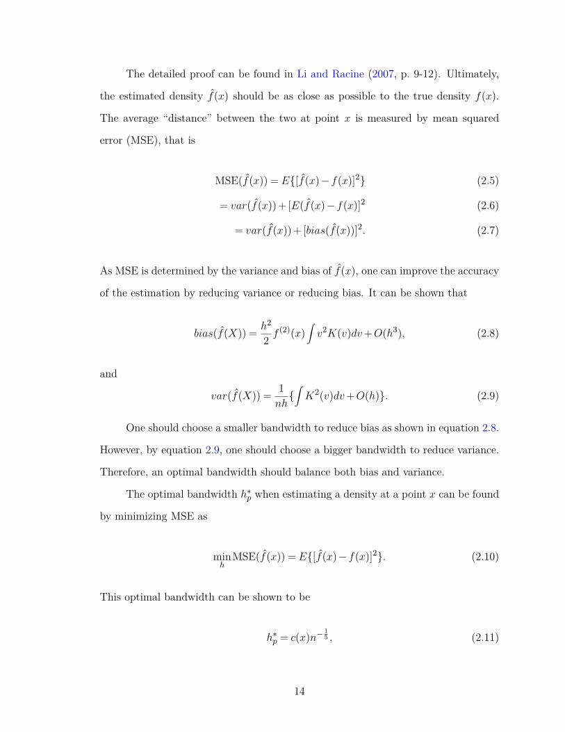
The detailed proof can be found in Li and Racine (2007, p. 9-12). Ultimately,
the estimated density f(x) should be as close as possible to the true density f(x).
The average “distance” between the two at point x is measured by mean squared
error (MSE), that is
MSE(f(x)) = E{[f(x)−f(x)]2} (2.5)
= var(f(x)) + [E(f(x)−f(x)]2 (2.6)
= var(f(x)) + [bias(f(x))]2. (2.7)
As MSE is determined by the variance and bias of f(x), one can improve the accuracy
of the estimation by reducing variance or reducing bias. It can be shown that
bias(f(X)) = h2
2 f(2)(x)
∫v2K(v)dv+O(h3), (2.8)
and
var(f(X)) = 1nh{∫K2(v)dv+O(h)}. (2.9)
One should choose a smaller bandwidth to reduce bias as shown in equation 2.8.
However, by equation 2.9, one should choose a bigger bandwidth to reduce variance.
Therefore, an optimal bandwidth should balance both bias and variance.
The optimal bandwidth h∗p when estimating a density at a point x can be found
by minimizing MSE as
minh
MSE(f(x)) = E{[f(x)−f(x)]2}. (2.10)
This optimal bandwidth can be shown to be
h∗p = c(x)n−15 , (2.11)
14

where c(x) = {κf(x)/[κ2f (2)(x)]2} 15 , κ2 =
∫v2K(v)dv and κ =
∫K2(v)dv. Alterna-
tively, if one is interested in the overall fit of f(x) on f(x), the optimal bandwidth h∗g
can be found by minimizing the integrated mean squared error (IMSE) in
minh
IMSE(f(x)) =∫E{[f(x)−f(x)]2}dx (2.12)
= 14h
4κ22
∫[f2(x)]2dx+ κ
nh+o(h4 + (nh)−1). (2.13)
The optimal bandwidth can be shown to be
h∗g = c0n− 1
5 , (2.14)
where c0 = {κ−2/52 κ1/5{
∫[f (2)(x)]2dx}− 1
5 > 0 is a positive constant.
Banwidth Selection
It is well-documented in the literature that the selection of the shape of the ker-
nel function has little impact on the estimated density (Silverman, 1986; Wand and
Jones, 1994; Lindström, Håkansson, and Wennergren, 2011). Therefore, instead of
Epanechnikov, Biweight, Triweight, Triangular, and Uniform, the standard Gaussian
is used as the kernel function throughout this research.
However, the bandwidth has a great influence on the estimated density. It’s
vital to choose appropriate bandwidth in nonparametric estimation. The relation-
ship between the size of the bandwidth and the shape of the estimated density is
demonstrated in figure 2.3: the larger the bandwidth, the smoother the estimated
density. There are three ways for bandwidth selection: (i) rule-of-thumb and plug-in
methods, (ii) least squares cross-validation methods, (iii) and maximum likelihood
cross-validation methods.
Rule-of-thumb and plug-in methods
Equation 2.14 shows that the optimal bandwidth depends on∫
[f2(x)]2dx. Instead
15

−4 −2 0 2 4
0.00
0.05
0.10
0.15
0.20
0.25
0.30
Grid
Den
sity
h=3
h=1
h=0.5
Figure 2.3: Changing bandwidth and the corresponding estimated density
of estimating, one might assume an initial value of h to estimate∫
[f2(x)]2dx non-
parametrically. The estimated value would then be plugged into equation 2.14 to
obtain the optimal h. Silverman (1986) suggested that we can assume f(x) be-
longs to a parametric family of distributions and then calculate the optimal h by
equation 2.14. If one assumes the true distribution is normal with variance σ2, then∫[f2(x)]2dx= 3/(8π1/2σ5).When a standard normal kernel is used, the pilot estimate
of bandwidth is
hpilot = (4π)−1/10[(3/8)π−1/2]−1/5σn−1/5 ≈ 1.06σn−1/5.
hpilot is then used in∫
[f2(x)]2dx to obtain the optimal bandwidth.
In practice, when the underlying distribution is similar to a normal distribu-
tion, hpilot might be directly used as the bandwidth. σ is replaced by the sample
standard deviation. Rule-of-thumb method is certainly easy to implement, but the
16

disadvantage is also clear: it is not fully automatic as one needs to manually choose
the initial h. The automatic or data-driven methods are discussed as follows.
Least squares cross-validation methods
Least squares cross-validation was proposed by Rudemo (1982), Stone (1984)
and Bowman (1984) to select a bandwidth which minimizes the integrated squared
error. That is a single bandwidth for all x in the support of f(x). The integrated
squared error is
∫[f(x)−f(x)]2dx=
∫f(x)2dx−2
∫f(x)f(x)dx+
∫f(x)2dx. (2.15)
Notice f(x) is a function of h, but true density f(x) is not. Thus the last term on the
right-hand side of equation 2.15 is unrelated to h. So the problem at hand is reduced
to
minh{∫f(x)2dx−2
∫f(x)f(x)dx}. (2.16)
∫f(x)f(x)dx can be estimated by
1n
n∑i=1
f−i(Xi), (2.17)
where
f−i(Xi) = 1(n−1)h
n∑j=1,j 6=i
K(Xi−Xj
h). (2.18)
And∫f(x)2dx can be estimated by
∫f(x)2dx = 1
n2h2
n∑i=1
n∑j=1
∫K(Xi−x
h)K(Xj−x
h)dx (2.19)
= 1n2h
n∑i=1
n∑j=1
K(Xi−Xj
h), (2.20)
where K(v) =∫K(u)K(v−u)du is the twofold convolution kernel derived from K(·).
17

Maximum likelihood cross-validation methods
Proposed by Duin (1976), likelihood cross-validation chooses h to maximize the
(leave-one-out) log likelihood function
L= lnL=n∑i=1
lnf−i(Xi), (2.21)
where
f−i(Xi) = 1(n−1)h
n∑j=1,j 6=i
K(Xj−Xi
h). (2.22)
The intuition of this method could be interpreted in this way: we first leave sample
point Xi out, and use the rest n− 1 sample points to estimate the probability that
sample Xi occurs (denoted by f−i(Xi)). We repeat this for i= 1,2, · · · ,n. Then
n∏i=1
f−i(Xi) = P (X1)×P (X2)×·· ·×P (Xn) (2.23)
represents the estimated probability from all sample points (X1,X2, · · · ,Xn). The
optimal h should maximize the product ∏ni=1 f−i(Xi). Because Likelihood cross-
validation is both intuitive and easy to implement, it is adopted as the bandwidth
selection method throughout this research.
2.3.2 Empirical Bayes Nonparametric Kernel Density Esti-
mator
Notice in the standard kernel density estimator, we only utilize n samples from one
column in our data matrix. However, the other Q− 1 columns of data might come
from similar densities and contain useful information. Ker and Ergün (2005) proposed
empirical Bayes nonparametric kernel density (EBayes) estimation method to exploit
the potential similarities among the Q densities (note each column in the data matrix
is from one density). The advantage of this method is that it can be applied to the
18

case where the form or extent of the similarities is unknown.
The empirical Bayes nonparametric kernel density estimator at support x for
experiment unit (i.e. county) i is
fEBi = fi
(τ2
τ2 +σ2i
)+µ
(σ2i
τ2 +σ2i
), (2.24)
where fEBi is the estimated density for county i, fi is the KDE for county i, µ,τ2,σ2i
are parameters to estimate, µ = (1/Q)∑Qi=1 fi, τ2 is the variance of the mean of
fi, τ2 = s2− (1/Q)∑Qi=1 σ
2i and s2 = (1/(Q−1))∑Q
i=1(fi− µ
)2, σ2
i is attained by
bootstrap.
Intuitively, the EBayes estimator is a weighted sum of two components: one is
KDE of county i (fi), and the other is the mean of KDEs of all Q counties (µ). The
weight given to the KDE of county i is w = τ2
τ2+σ2i. And the weight 1−w = σ2
i
τ2+σ2iis
given to the mean density µ. When the variance of the estimated densities across the
experiment units (i.e. counties) increases (τ2 ↑) , the EBayes estimator will shrink
towards the KDE. This is reasonable; because as the variance across counties increase,
underline densities of each county are more likely to be different. At this time,
incorporating information from other counties is more likely to add “noise” rather
than improve the estimation efficiency. Therefore, the information from the own
county should be given more weight. Conversely, when the variance of the estimated
densities within the county is relatively high, more weight should be given to the
overall mean density µ. The reason is that, as there are less variance across counties,
it is more likely that the underline densities for each county are similar. Both Ker
and Ergün (2005) and Ramadan (2011) provided evidence that EBayes has improved
performance than KDE when the underline densities are of similar structure.
19

2.3.3 Conditional Density Estimator
Hall, Racine, and Li (2004) proposed the conditional density estimator. Instead of
applying KDE on a county-to-county basis to estimate densities, Racine and Ker
(2006) used conditional density estimator to estimate yield densities jointly across
counties. Their approach incorporates discrete data (the counties where the yield
data is recorded) into the standard kernel density estimator. I denote this method as
Cond in this thesis. Recall that in KDE there is only one bandwidth smoothing yield
data from its own county. Cond contains two; one bandwidth smooths continuous
yield data, the other smooths discrete data (the counties). Comparing to KDE, this
method adds another dimension: the counties. Thus Cond smooths data both within
and across counties. It is done by pooling all observations together, but weighting
those from the own county and those from other counties differently. The benefits of
doing so are: (a) borrowed information from extraneous counties may help to improve
estimation efficiency. And (b) the “noise” (yield data from other counties when their
densities are very dissimilar) can be controlled by adjusting the weight (λ) given to
the extraneous counties.
Mathematically, it is implemented in the following way.
fCond (x|Cj) = fCond (Cj ,x)m(Cj)
, (2.25)
where fCond (x|Cj) is the conditional density estimator, representing the estimated
density of x (yield) conditional on Cj (county). And
fCond (Cj ,x) = 1nQ
nQ∑l=1
Kd(cl,Cj)L(x,Xl) = 1nQhC
nQ∑l=1
Kd (cl,Cj)K(x−Xl
hC),
20

Kd (cl,Cj) =(
λ
Q−1
)N(cl,Cj)(1−λ)1−N(cl,Cj) ,
0≤ λ≤ Q−1Q is the weight, N (cl,Cj) =
0 if cl = Cj
1 if cl 6= Cj ,
and m(Cj) = 1nQ
∑nQi=1K
d (cl,Cj)≡ 1Q , that is
fCond(x|Cj) = 1nhC
n∑l=1
(1−λ)K(x−XCj
l
hC)︸ ︷︷ ︸
Own county
+n(Q−1)∑l=1
λ
Q−1K(x−XC−j
l
hC)︸ ︷︷ ︸
Extraneous Counties
.
It’s more clear to see how Cond is related to KDE in the following example.
Suppose we are estimating yield density for county 1. That is Cj = C1, then
fCond(x|C1) = 1nhC
n∑l=1
(1−λ)K(x−XC1l
hC)︸ ︷︷ ︸
County 1
+n(Q−1)∑l=1
λ
Q−1K(x−XC−1l
hC)︸ ︷︷ ︸
County 2, 3, · · · , Q
.
In the first case, let’s assume λ = 0. Then the weight given to yield data from
C1 (own county) is 1 and to yield data from extraneous counties (county 2, 3, · · · , Q)
is 0. In this case, the conditional density estimator converges to KDE.
In the second case, assume λ = Q−1Q , then the weight given to yield data from
the own county is 1−λ= 1Q . And the weight given to other counties is also λ
Q−1 = 1Q .
As data from all counties are getting the same weight, the conditional estimator
converges to a KDE that uses data from all counties.
Notice these two cases are representing the upper and lower limit of λ (0 ≤
λ ≤ Q−1Q ). For any other λ that’s between 0 and Q−1
Q , Cond essentially mixes data
from different sources. As discussed before, if the densities of the other counties are
very different from the own county, Cond assigns a small (or 0) weight to extraneous
21

data; the external information is more likely to be “noise” any way. If, on the other
hand, the densities of the other counties are similar (or identical) to that of the
own county, Cond assigns similar (or identical) weight to extraneous information.
Particularly, when all Q densities are identical, assign the same weight to data from
different counties will pool all data together. This will increase the sample size and
improve the estimation efficiency. The discussion here is demonstrated in an example
in Appendix 6.2.
2.3.4 Jones Bias Reduction Estimator
Jones, Linton, and Nielsen (1995) proposed a bias reduction method for kernel density
estimation (denoted as Jones). It is
fJones(x) = f(x) 1nhJ
n∑i=1
K(x−XCji
hJ)
f(XCj
i
) , (2.26)
where K(·) is the standard Gaussian kernel function with bandwidth hJ . f(x) =1
nhJp
∑nl=1K(x−X
Cjl
hJp), the pilot, is the estimated density via KDE method where band-
width is hJp. Notice all the data used here are from Cj , the own county. When the
bandwidth of the pilot (hJp) is very large, the pilot shrinks to uniform distribution
and fJones reduces to KDE. The intuition of this method is that it assumes the
relationship between the true density ft(x) and the estimated density fe(x) is
fe(x) = ft(x)α(x), (2.27)
where α(x) = fe(x)/ft(x) is a multiplicative bias correction term. And α(x) is esti-
mated by
α(x) = 1nh
∑K(x−Xih )
f(Xi).
22

2.3.5 Possibly Similar Estimator
Notice in the Jones, we only utilize a sample of size n from one column in the data
matrix. However, the other Q−1 columns of data might come from similar densities
and contain useful information. Such information might be helpful in estimating
the density of interest. Especially, if the other Q− 1 columns of data is also known
to be from the same density, it would be logical to pool all data together before
estimation. Ker (2014) proposed a possibly similar estimator (denoted as KerPS)
that was designed to estimate a set of densities of possibly similar structure. The
estimated density at x is
fKerPS(x) = g(x) 1nhK
n∑i=1
K(x−XCji
hK)
g(XCj
i ), (2.28)
where g(x) = 1nQhKp
∑nQl=1K(x−Xl
hKp), K(·) is the standard Gaussian kernel function
with bandwidth hK , g(·) is estimated with KDE method by pooling data from all
counties together with bandwidth hKp. Similar to Jones, when the bandwidth of the
pilot (hKp) is very large, the pilot shrinks to uniform distribution and fKer(x) reduces
to KDE. One can think of this estimator as a fashion of Hjort and Glad (1995). That
is, nonparametrically correct a nonparametric pilot estimator (Ker, 2014). g(x) is the
pilot estimator with pooled data from all counties. And
1nhK
n∑i=1
K(x−XCji
hK)
g(XCj
i )
is a nonparametric correction term. Or one can think of this estimator in a fashion
of Jones, Linton, and Nielsen (1995) where the multiplicative bias correction term is
αKer(x) = 1nhK
n∑i=1
K(x−XCji
hK)
g(XCj
i ),
23

and
f(x)KerPS = g(x)×αKer(x) (2.29)
It should be noted that KerPS is designed for situations where the underlying
densities are thought to be identical or similar. Because with identical or similar
densities, the pooled estimator is a reasonable start. However, Ker (2014) showed
that KerPS didn’t seem to lose any efficiency even if the underlying densities were
dissimilar. The reason is similar to Hjort and Glad (1995): reduce bias by reducing
global curvature of the underlying function being estimated. KerPS pools all data
together to form a start. By utilizing extraneous data, the total curvature that is
being estimated might be greatly reduced, resulting reduced bias.
2.4 Summary
This chapter reviews the parametric, semiparametric and nonparametric density esti-
mation methods. Normal, Beta and Weibull distributions are often used to character-
ize the crop yield data-generating process. The parametric estimators converge to the
true densities at a higher rate comparing to nonparametric estimators when the prior
assumption of parametric family is correct. But misspecification leads to inconsistent
density estimation. Semiparametric methods combine the high convergence rate of
parametric methods with flexibility of nonparametric methods. Nonparametric meth-
ods do not require prior assumption of the distribution family. The standard kernel
density estimator, the empirical Bayes nonparametric kernel density estimator, the
conditional density estimator, the Jones bias reduction method and the Ker’s possibly
similar estimator are discussed. The integrated mean squared error, a summation of
estimation bias and variance term, measures the density estimation efficiency. One
can select bandwidth to reduce bias, variance or both to improve the density estima-
tion efficiency. To select a bandwidth in practice, one can use rule-of-thumb, least
24

squares cross-validation or maximum likelihood cross-validation.
The standard kernel density estimator has no bias or variance reduction term.
The empirical Bayes nonparametric kernel density estimator can potentially reduce
estimation variance, especially when the set of densities in the study are similar. The
conditional density estimator reduces estimation variance; in the cross-validation pro-
cess, large smoothing parameters are assigned to irrelevant components, suppressing
their contribution to estimator variance. Jones bias reduction method improves es-
timation efficiency by a multiplicative bias reduction term using data from the own
county. Ker’s possibly similar estimator, resembling Jones bias reduction method,
also contains a multiplicative bias reduction term but with a pooled estimate replac-
ing the pilot estimate in Jones.
25

Chapter 3
Proposed Estimators
Recall that mean squared error is
MSE(f(x)) = E{[f(x)−f(x)]2}
= var(f(x)) + [E(f(x)−f(x)]2
= var(f(x)) + [bias(f(x))]2,
a summation of a variance term and a bias term. Therefore, there are three ways to
improve the estimation efficiency: reducing bias, reducing variance or reducing both.
KerPS is a bias reduction method where bias reduction is realized by a multiplicative
bias correction term as shown in equation 2.29. As crop reporting districts represent
divisions of approximately equal size with similar soil, growing conditions and types
of farms, it is likely that each individual county’s yields are similar in structure. As
discussed before, Ker (2014) showed that the possibly similar estimator offered greater
efficiency if the set of densities were similar while seemingly not losing any if the set
of densities were dissimilar. However, the possibly similar estimator is designed for
situations where the underline densities are suspected to be similar, efficiency loss,
regardless of the magnitude, is inevitable when it is wrongly applied to situations
with dissimilar densities. Unfortunately, under most (if not all) empirical settings,
one can not know the structure of true densities with certainty. It might be beneficial
to have an estimator which preserves the bias reduction capability of KerPS and also
reduces variance.
Cond is a variance reduction method. When estimating conditional densities,
26

explanatory variables may have both relevant and irrelevant components. Cross-
validation in Cond can automatically identify which components are relevant and
which are not. Large smoothing parameters are assigned to the irrelevant compo-
nents shrinking their distributions to uniform, the least-variable distribution. Thus
the irrelevant components contribute little to the variance term of the Cond density
estimator, resulting an overall decreased variance. Note the irrelevant components
have little impact on the bias of Cond density estimator; the fact that they are irrel-
evant implies that they contain little information about the explained variable (Hall,
Racine, and Li, 2004).
Naturally, a combined method that reduces both bias and variance is desirable.
I propose two new estimators that are designed with this goal in mind: reducing
both bias and variance yet requiring no prior knowledge of the structure of the true
densities. Figure 3.1 illustrates how the bias reduction method and the variance
reduction method are combined to form the two new estimators. Starting from KDE
which has no bias or variance reduction term, Jones and KerPS add multiplicative bias
reduction term and Cond adds variance reduction capability. There are two ways to
combine bias reduction with variance reduction: introduce variance reduction term
from Cond into bias-reducing KerPS (which forms the new estimator Comb1), or
bias reduction term from KerPS into variance-reducing Cond (which forms the new
estimator Comb2). Although Jones and KerPS are both bias reduction methods, I
combine KerPS, instead of Jones, with Cond to offer more flexibility. Note Jones uses
data only from the own county and KerPS uses data from all counties.
The two proposed estimators are straight forward and intuitive. Comb1, the first
proposed estimator, combines the conditional estimator into Ker’s possibly similar
estimator. As a result, Comb1 is a generalized form which can shrink back to KDE,
Jones or KerPS under different conditions. In other words, KDE, Jones and KerPS
are three special cases of the proposed Comb1 method. Comb2, the second proposed
27

KDE
Jones
Comb2
Comb1
Cond
KerPS
+ b
ias reduct
ion
+ bias reduction
+ variance reduction
Figure 3.1: Combining bias and variance reduction method to form Comb1 andComb2
estimator, combines KerPS into conditional estimator in a different way. As a result,
Comb2 is a generalized form which can shrink back to KDE, KerPS or Cond under
different conditions. That is, KDE, KerPS and Cond are special cases of Comb2.
Instead of just reducing bias or variance, the two proposed estimators reduce
both. Given the optimal bandwidths, Comb1 can always outperform KDE, Jones and
KerPS. Similarly, Comb2 can potentially outperform KDE, Cond and KerPS if the
optimal bandwidths are known. This is because KDE, Jones and KerPS are special
cases of Comb1 and KDE, Cond and KerPS are special cases of Comb2. Comb1 and
Comb2 can always shrink back to their special cases by restricting the corresponding
bandwidth(s). However, in empirical settings where the optimal bandwidths are
unknown, it should be noted that Comb1 and Comb2 do not always perform better
than their special cases. It should also be noted that the two proposed estimators
are more computationally demanding because of the additional bandwidth. In the
following two sections, I discuss the two proposed estimators in detail.
28

3.1 Comb1
Recall that KerPS estimator is
fKerPS(x) = g(x) 1nhK
n∑i=1
K(x−XCji
hK)
g(XCj
i )(3.1)
where g(·) is a nonparametric start with data from all counties. KerPS is expected
to improve estimation efficiency if the true density of all counties are of identical
or similar structure. However, if the true densities are dissimilar, pooling all data
together to form a start may include undesirable information from a very dissimilar
distribution. Logically, in such scenario, one should only use data from its own county.
Ideally, in a more flexible estimator, one can pool all data together to form a
start as Ker (2014) if the true densities are similar, or just use data from the own
county to form a start as Jones, Linton, and Nielsen (1995) if the true densities are
dissimilar. Comb1 is constructed to offer exactly that flexibility. It is straightforward
and intuitive. I replace the g (.) in KerPS by a conditional estimator component
gcb1 (.). The density of yield x in county Cj estimated by Comb1 estimator is then
fcb1(x) = 1nhcb1
n∑i=1
K(x−XCji
hcb1)
gcb1(XCj
i )gcb1(x),
Kd (cl,Cj) =(
λ
Q−1
)N(cl,Cj)(1−λ)1−N(cl,Cj) ,
29

0≤ λ≤ Q−1Q , N (cl,Cj) =
0 if cl = Cj
1 if cl 6= Cj ,
and
gcb1(x) = 1nhp
nQ∑l=1
Kd (cl,Cj)K(x−Xl
hp)
= 1nhp
n∑l=1
(1−λ)K(x−XCj
l
hp)︸ ︷︷ ︸
Own county
+n(Q−1)∑l=1
λ
Q−1K(x−XC−j
l
hp)︸ ︷︷ ︸
Extraneous Counties
.
Notice the only difference between Comb1 and KerPS is the weight term Kd(cl,Cj).
By introducing such a weight, Comb1 is a flexible general estimator which can shrink
back to KerPS or Jones. This is done by setting λ to its upper or lower boundary.
Firstly, suppose λ gets the lower boundary value 0. In this case, Kd(cl,Cj) is 1 for
the own county and 0 for the extraneous counties. This will reduce gcb1(x) down
to the kernel estimator with data only from own county. As a result, the Comb1
estimator shrinks back to Jones. Secondly, let’s suppose λ gets the upper boundary
value of Q−1Q . In this case, Kd(cl,Cj) = 1
Q for every county, no matter it is the own
county or extraneous counties. This is identical to pooling all data from all counties
together. As a result, the Comb1 estimator shrinks back to KerPS. Lastly, if gcb1(x)
is uniformly distributed (or, hp→∞), then gcb1(x) ≡ gcb1(Xi) ∀ i. In this case, the
Comb1 estimator shrinks back to the standard kernel estimator with data from its
own county. For any other 0< λ < Q−1Q , Comb1 assigns weight 1−λ to observations
from its own county and weight λQ−1 to observations from other counties.
By introducing a weighting term Kd(cl,Ci), KDE, Jones and KerPS are en-
capsulated into one general estimator— the Comb1 estimator. This new proposed
estimator has the potential to perform better than KDE, Jones and KerPS. After all,
these three are special cases of Comb1. Additionally, Comb1 reduces not only bias but
also variance. By a weigh 0 < λ < Q−1Q , Comb1 can potentially improve estimation
30

efficiency to a higher level that can not be reached by KDE, Jones or KerPS. The
relationship between KDE, Jones and KerPS is shown in the upper part of figure 3.2.
3.2 Comb2
Recall that in conditional estimator, the numerator is
fCond (Cj ,x) = 1nQ
nQ∑l=1
Kd(cl,Cj)L(x,Xl) (3.2)
where L(x,Xl) is the kernel estimator with data from all counties. Similar to Jones,
Linton, and Nielsen (1995) and Ker (2014), I introduce a bias correction term into
this numerator to form Comb2, the second proposed estimator. That is, L(x,Xi)
will be replaced by gcb2(x) L(x,Xl)gcb2(Xl) . One can interpret L(x,Xl)
gcb2(Xl) as a multiplicative
bias correction term as in Jones, Linton, and Nielsen (1995). Or as Ker (2014), one
can think gcb2(x) as a nonparametric start, and the term L(x,Xl)gcb2(Xl) nonparametrically
corrects this start.
The second proposed estimator, Comb2 is then
fcb2(x|Cj) = fcb2(Cj ,x)m(Cj)
, (3.3)
fcb2(Cj ,x) = 1nQ
nQ∑l=1
Kd(cl,Cj)L(x,Xl)gcb2(Xl)
gcb2(x), (3.4)
Kd (cl,Cj) =(
λ
Q−1
)N(cl,Cj)(1−λ)1−N(cl,Cj) , (3.5)
L(x,Xl) = 1hcb2
K(x−Xl
hcb2), (3.6)
gcb2(x) = 1nQhg
nQ∑j=1
K(x−Xj
hg), (3.7)
31

and 0≤ λ≤ Q−1Q , N (cl,Cj) =
0 if cl = Cj
1 if cl 6= Cj ,
and m(Cj) = 1nQ
∑nQi=1K
d (cl,Cj)≡ 1Q ,
that is,
fcb2(x|Cj) = 1nhcb2
n∑l=1
(1−λ)K(x−X
Cjl
hcb2)
gcb2(XCj
l )gcb2(x)
︸ ︷︷ ︸Own county
+n(Q−1)∑l=1
λ
Q−1K(x−X
C−jl
hcb2)
gcb2(XC−j
l )gcb2(x)
︸ ︷︷ ︸Extraneous Counties
.(3.8)
Comparing to Cond, Comb2 is different by the bias correction term. As a result
of this modification, KDE, KerPS and Cond are all encapsulated into one general
form—the proposed Comb2 estimator.
Intuition to understand the connections between KDE, KerPS, Cond and Comb2
are provided as follows. Firstly, suppose λ= 0 and the bandwidth in gcb2(·), hg→∞,
Comb2 will converge back to KDE. Essentially, by setting λ = 0, we are only using
data from the own county. And when hg →∞, gcb2(x) ≡ gcb2(Xl) ∀ l. So Comb2
will be identical to standard kernel method with data from its own county. Secondly,
when λ = 0 and hg is a small number, Kd(cl,Cj) will be 1 for the own county and
zero for all extraneous counties. Comb2 will shrink back to KerPS. Thirdly, suppose
hg→∞, then gcb2(x)≡ gcb2(Xl) ∀ l and cancels out in equation 3.8. Thus Comb2 will
converge back to Cond. The relationship between KDE, KerPS and Cond is shown
in the lower part of figure 3.2.
By introducing a multiplicative bias correction term, KDE, KerPS and Cond
are encapsulated into another general estimator— Comb2 estimator. If the optimal
bandwidths are known, this proposed estimator should perform, at least, better than
KDE, KerPS and Cond. And by selecting a weight 0 < λ < Q−1Q and a bandwidth
hg sufficiently small, Comb2 can potentially improve estimation efficiency to a higher
level which can not be reached by KDE, KerPS or Cond. Note that the optimal
32

KDE
Jones
Comb2
Comb1
Cond
KerPS
( ), ,
( ),,
( ),
,
,
( )
( )
( )
Note: The bandwidths of each method are in the parentheses. When the bandwidths satisfy condi-tions on the arrow, the estimator converges back to the previous one.
Figure 3.2: The relationship between the estimators
bandwidths are rarely known in empirical settings, thus Comb2 might not always
outperform its special cases in empirical applications.
3.3 Proofs
Theorem 1. KDE, Jones and KerPS are special cases of Comb1.
Lemma 3.3.1. If hp→∞ and hcb1 = h, then fcb1(x) = fKDE(x)
Proof. If hp→∞, then
gcb1(x) = 1nhp
nQ∑l=1
Kd(cl,Cj)K(x−Xl
hp
)≈ 1nhp
nQ∑l=1
Kd(cl,Cj)K(0),
33

and
gcb1(XCj
i ) = 1nhp
nQ∑l=1
Kd(cl,Cj)KXCj
i −Xl
hp
≈ 1nhp
nQ∑l=1
Kd(cl,Cj)K(0),
thus, gcb1(x) = gcb1(XCj
i ) and gcb1(x) is density function of an uniform distribution.
Then
fcb1(x) = 1nhcb1
n∑i=1
K
x−XCj
i
hcb1
,and if hcb1 = h, then
fcb1(x) = 1nh
n∑i=1
K
x−XCj
i
h
= fKDE(x).
Lemma 3.3.2. If λ= 0, hp = hJp and hcb1 = hJ , then fcb1(x) = fJones(x)
Proof. If λ= 0, then Kd(cl,Ci) = 0N(cl,Cj)11−N(cl,Cj) =
1 if cl = Cj
0 if cl 6= Cj
, and
gcb1(x) = 1nhp
n∑i=1
1×Kx−XCj
i
hp
+n(Q−1)∑i=1
0×Kx−XC−j
i
hp
(3.9)
= 1nhp
n∑i=1
K
x−XCj
i
hp
. (3.10)
If hp = hJp, gcb1(x) = f(x) and gcb1(XCj
i ) = f(XCj
i ), thus
fcb1(x) = 1nhcb1
n∑i=1
K(x−XCji
hcb1)
f(XCj
i )f(x),
34

and if hcb1 = hJ ,
fcb1(x) = 1nhJ
n∑i=1
K(x−XCji
hJ)
f(XCj
i )f(x) = fJones(x)
Lemma 3.3.3. If λ= Q−1Q , hp = hKp and hcb1 = hK , then fcb1(x) = fKerPS(x)
Proof. If λ= Q−1Q , then λ
Q−1 = 1−λ= 1Q ,
Kd(cl,Ci) = 1Q
N(cl,Cj) 1Q
1−N(cl,Cj) =
1Q if cl = Cj
1Q if cl 6= Cj
, thus
gcb1(x) = 1nhp
n∑l=1
1Q×K
x−XCj
l
hp
+n(Q−1)∑l=1
1Q×K
x−XC−j
l
hp
= 1nQhp
nQ∑l=1
K
(x−Xl
hp
).
If hp = hKp, gcb1(x) = 1nQhKp
∑nQl=1K(x−Xl
hKp) = g(x) and gcb1(XCj
i ) = g(XCj
i ), thus
fcb1(x) = 1nhcb1
n∑i=1
K(x−XCji
hcb1)
g(XCj
i )g(x),
and if hcb1 = hK , then
fcb1(x) = 1nhK
n∑i=1
K(x−XCji
hK)
g(XCj
i )g(x) = fKerPS(x)
Theorem 2. KDE, Cond and KerPS are special cases of Comb2.
Lemma 3.3.4. If hg→∞, λ= 0 and hcb2 = h, then fcb2(x|Cj) = fKDE(x)
35

Proof. If hg→∞, then
gcb2(x) = 1nQhg
nQ∑j=1
K
(x−Xj
hg
)≈ 1nQhg
nQ∑j=1
K(0),
and
gcb2(Xl) = 1nQhg
nQ∑j=1
K
(Xl−Xj
hg
)≈ 1nQhg
nQ∑j=1
K(0),
thus gcb2(x) = gcb2(Xl) and gcb2(x) is density function of an uniform distribution.
Then
fcb2(Cj ,x) = 1nQ
nQ∑l=1
Kd(cl,Cj)L(x,Xl) = 1nQhcb2
nQ∑l=1
Kd(cl,Cj)K(x−Xl
hcb2)
and
fcb2(x|Cj) = fcb2(Cj ,x)m(Cj)
= 1nhcb2
nQ∑l=1
Kd(cl,Cj)K(x−Xl
hcb2).
If λ= 0, then Kd(cl,Ci) = 0N(cl,Cj)11−N(cl,Cj) =
1 if cl = Ci
0 if cl 6= Ci
,
fcb2(x|Cj) = 1nhcb2
n∑l=1
1×Kx−XCj
l
hcb2
+n(Q−1)∑l=1
0×Kx−XC−j
l
hcb2
= 1nhcb2
n∑l=1
K
x−XCj
l
hcb2
.And if hcb2 = h, then
fcb2(x|Cj) = 1nh
n∑l=1
K
x−XCj
l
h
= fKDE(x)
Lemma 3.3.5. If hg→∞ and hcb2 = hC , then fcb2(x|Cj) = fCond(x|Cj)
36

Proof. If hg→∞, then
gcb2(x) = 1nQhg
nQ∑j=1
K(x−Xj
hg)≈ 1
nQhg
nQ∑j=1
K(0),
and
gcb2(Xl) = 1nQhg
nQ∑j=1
K(Xl−Xj
hg)≈ 1
nQhg
nQ∑j=1
K(0),
thus gcb2(x) = gcb2(Xl) and gcb2(x) is density function of an uniform distribution.
Then
fcb2(Cj ,x) = 1nQ
nQ∑l=1
Kd(cl,Cj)L(x,Xl) = 1nQhcb2
nQ∑l=1
Kd(cl,Cj)K(x−Xl
hcb2
)
and
fcb2(x|Cj) = fcb2(Cj ,x)m(Cj)
= 1nhcb2
nQ∑l=1
Kd(cl,Cj)K(x−Xl
hcb2
).
And if hcb2 = hC , then
fcb2(x|Cj) = 1nhC
nQ∑l=1
Kd(cl,Cj)K(x−Xl
hC
)= fCond(x|Cj)
Lemma 3.3.6. If λ= 0, hg = hKp, and hcb2 = hK , then fcb2(x|Cj) = fKerPS(x)
Proof. If λ= 0, then Kd(cl,Ci) = 0N(cl,Cj)11−N(cl,Cj) =
1 if cl = Ci
0 if cl 6= Ci
,
fcb2(Cj ,x) = 1nQhcb2
n∑l=1
1×K(x−X
Cjl
hcb2)
gcb2(XCj
l )gcb2(x) +
n∑l=1
0×K(x−X
C−jl
hcb2)
gcb2(XC−j
l )gcb2(x)
= 1nQhcb2
n∑l=1
K(x−XCjl
hcb2)
gcb2(XCj
l )gcb2(x),
37

and
fcb2(x|Cj) = 1nhcb2
n∑l=1
K(x−XCjl
hcb2)
gcb2(XCj
l )gcb2(x).
If hg = hKp, then gcb2(x) = g(x) and gcb2(XCj
l ) = g(XCj
l ).
Lastly, if hcb2 = hK , then
fcb2(x|Cj) = 1nhK
n∑l=1
K(x−XCjl
hK)
g(XCj
l )g(x) = fKerPS(x).
3.4 Summary
There are three ways to improve the efficiency of nonparametric density estimators:
reducing bias, reducing variance or reducing both. KerPS is a bias reduction method
by employing a multiplicative bias correction term. Cond is a variance reduction
method; estimation variance is reduced by assigning large bandwidth to irrelevant
components. Combining bias reduction and variance reduction methods into one es-
timator could potentially increase the estimation efficiency significantly. This chapter
introduces two new proposed estimators, Comb1 and Comb2, that reduce both bias
and variance.
Comb1 introduces a variance reduction weighting term from Cond into bias-
reducing KerPS. When the yields from extraneous counties are from very dissimilar
densities, the weighting term enables Comb1 to ignore the undesirable extraneous
information. As a result, the estimation variance is reduced. In this case, Comb1
acts like Jones, using information only from the own county. When the yields are
from similar densities, the weighting term can enable Comb1 to act like KerPS, using
information from all counties. Comb1 may potentially outperform KDE, Jones and
38

KerPS. Not only because that these three are all special cases of Comb1 but also that
Comb1 reduces both estimation bias and variance.
Different from Comb1, Comb2 introduces a multiplicative bias reduction term
from KerPS into variance-reducing Cond. As a result, Comb2 has the ability to reduce
both variance and bias. Comb2 is a generalized estimator containing KDE, KerPS
and Cond as special cases. Comb2 may potentially outperform KDE, KerPS and
Cond. Because comparing to KDE, it has the additional bias reduction and variance
reduction capacity; comparing to bias-reducing KerPS, it has the additional variance
reduction capacity and comparing to variance-reducing Cond, it has the additional
bias reduction capacity.
39

Chapter 4
Simulation
Chapter 3 argued that the two proposed new estimators, Comb1 and Comb2, could
have promising efficiency improvement. This chapter compares the performance of
the two proposed estimators to KDE, Ebayes, Cond, and KerPS by simulation. The
chapter is organized as follows. First, the criterion which measures the performance
of each estimator is described. Then several estimation considerations are discussed.
Finally the simulation results are reported in two sections: i) when the true densities
are known and ii) when the true densities are unknown. In each section, the simulation
is run in three different scenarios: a) dissimilar true densities; b) moderately similar
true densities; and c) identical true densities.
The simulation where the true densities are known can directly demonstrate
the performance of each methods. As the true densities are known, the distance
between each estimator and the true density can be measured. The closer the dis-
tance, the better the estimator. However, in empirical settings, the true densities are
rarely known. The simulation where the true densities are unknown is designed to
demonstrate the performance of each estimator in empirical applications.
The performance of each density estimator is measured by its distance away
from the true density. In figure 4.1, the solid line is the true density and the dashed
line is the estimated density. The shadow area represents the distance between the
two and thus is a measure of the performance of the estimator. The smaller the
area, the better the estimator performs. Mathematically, the area is measured by
40

True DensityEstimated Density
Figure 4.1: Integrated squared error illustration
integrated squared error (ISE) as
ISE =∫ (
f(x;h)−f(x))2dx, (4.1)
where f(x;h) is the estimated density, h is a vector of bandwidths and f(x) is the
true density. The ISE is used as a criterion to compare the performance of different
estimators in this thesis.
4.1 Some Considerations
There are some issues to consider before the simulation including bandwidth selection,
starting value, integration and density transformation.
Bandwidth Selection
As discussed before, when true densities are known, the bandwidths are selected to
minimize ISE. This is straightforward in KDE and EBayes estimator. In Cond, the
41

two bandwidths (λ,hC) are selected jointly in one optimization function to minimize
ISE. Note that λ is the parameter to smooth over counties and h is the parameter to
smooth over yields. In KerPS, there are two approaches to select the two bandwidths
(hK for the data of individual county and hKp for the pooled data). The first approach
chooses hK and hKp independently. hKp is chosen to minimize the ISE for the pooled
density g(·). That is
minhKp
ISEg =∫ (
g(x;hKp)−g(x))2dx. (4.2)
Then given the optimal hKp from this minimization, hK is chosen to minimize the
ISE of possibly similar estimator fKerPS . Alternatively, hK and hKp can be chosen
jointly to minimize the ISE of KerPS as in
minhKp,hK
ISEKerPS =∫ (
fKerPS(x;hK ,hKp)−fKerPS(x))2dx. (4.3)
Ker (2014) noticed that it might be appropriate to over-smooth and select a large
hKp. In Jones, the pilot density (the start) and the bias correction term share the
same bandwidth. Only one bandwidth is selected to minimize the ISE of Jones
estimator. The reason, as discussed in Jones, Linton, and Nielsen (1995), is that a
single bandwidth ensures the bias cancellation.
There are three bandwidths in both Comb1 and Comb2: hcb1, hp and λ for
Comb1 and hcb2, hg and λ for Comb2. hcb1 and hcb2 smooth data within an individual
sample (or county), hp and hg smooth the pooled data and λ to smooth between
different samples (or counties). All three bandwidths are chosen jointly as in
minhp,hcb1,λ
ISEComb1 =∫ (
fComb1(x;hcb1,hp,λ)−fComb1(x))2dx (4.4)
42

for Comb1 and
minhg,hcb2,λ
ISEComb2 =∫ (
fComb2(x;hcb2,hg,λ)−fComb2(x))2dx (4.5)
for Comb2.
Starting Value
Because there are three parameters to choose in Comb1 and Comb2, the optimiza-
tion process is time-consuming, especially when the sample size is large. Choosing
starting values close to the optimal bandwidths would reduce the calculation time.
The optimal bandwidths from Cond and KerPS are used as starting value for Comb1
and Comb2 in this thesis.
Integration
Some of the density estimators may not integrate to 1. In such a case, the estimator
is normalized to be able to integrate to 1. This is done as
fn(x) = f(x)∫f(x)dx
,
where fn(x) is the renormalized density which integrates to 1.
Density Transformation
In KerPS estimator, Ker (2014) proposed to transform the individual samples to have
mean 0 and variance 1. The density was estimated based on standardized data and
then back-transformed by the mean and variance of the sample. The reason is that
one can often accurately recover mean and variance even with small sample; and the
pooled data is only used to assist on estimating the shape of the density. I follow this
density transformation method in estimating KerPS, Comb1 and Comb2.
43
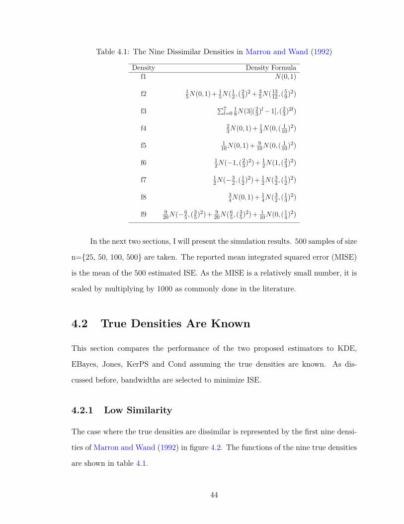
Table 4.1: The Nine Dissimilar Densities in Marron and Wand (1992)
Density Density Formulaf1 N(0,1)
f2 15N(0,1) + 1
5N(12 ,(
23)2 + 3
5N(1312 ,(
59)2)
f3 ∑7l=0
18N(3[(2
3)l−1],(23)2l)
f4 23N(0,1) + 1
3N(0,( 110)2)
f5 110N(0,1) + 9
10N(0,( 110)2)
f6 12N(−1,(2
3)2) + 12N(1,(2
3)2)
f7 12N(−3
2 ,(12)2) + 1
2N(32 ,(
12)2)
f8 34N(0,1) + 1
4N(32 ,(
13)2)
f9 920N(−6
5 ,(35)2) + 9
20N(65 ,(
35)2) + 1
10N(0,(14)2)
In the next two sections, I will present the simulation results. 500 samples of size
n={25, 50, 100, 500} are taken. The reported mean integrated squared error (MISE)
is the mean of the 500 estimated ISE. As the MISE is a relatively small number, it is
scaled by multiplying by 1000 as commonly done in the literature.
4.2 True Densities Are Known
This section compares the performance of the two proposed estimators to KDE,
EBayes, Jones, KerPS and Cond assuming the true densities are known. As dis-
cussed before, bandwidths are selected to minimize ISE.
4.2.1 Low Similarity
The case where the true densities are dissimilar is represented by the first nine densi-
ties of Marron and Wand (1992) in figure 4.2. The functions of the nine true densities
are shown in table 4.1.
44

−4 −2 0 2 4
0.0
0.1
0.2
0.3
0.4
(a) f1−4 −2 0 2 4
0.0
0.2
0.4
(b) f2−4 −2 0 2 4
0.0
0.4
0.8
1.2
(c) f3
−4 −2 0 2 4
0.0
0.5
1.0
1.5
(d) f4−4 −2 0 2 4
01
23
(e) f5−4 −2 0 2 4
0.00
0.10
0.20
0.30
(f) f6
−4 −2 0 2 4
0.0
0.1
0.2
0.3
0.4
(g) f7−4 −2 0 2 4
0.0
0.1
0.2
0.3
0.4
(h) f8−4 −2 0 2 4
0.00
0.10
0.20
0.30
(i) f9
Figure 4.2: The Nine Dissimilar Densities in Marron and Wand (1992)
45

The nine densities are very different from each other, representing a large variety
of density structures thus the worst scenario. In empirical settings, if the underlying
true density are believed to be as dissimilar as these nine, researchers would not think
of estimators such as KerPS, Comb1 or Comb2. Especially, as KerPS is designed to
borrow shapes from other densities, applying KerPS would borrow very different
shapes than the true density. However, more flexible estimators Comb1 and Comb2
would adjust itself to not borrow information under such scenario. Therefore, this is
an ideal setting where we can see the advantage of employing Comb1 and Comb2. It
should be noted that this low similarity scenario mimics a very harsh setting which
is used to test the limit of proposed estimators. If the proposed estimators yield
efficiency gain even in this scenario, they stand a good chance of performing well
under most circumstances.
The simulated results of the worst scenario are shown in table 4.2. Encouraging,
but as expected, the two new proposed estimators are able to yield lower MISE.
Comb1 as a general estimator outperforms its special cases KDE, Jones and KerPS.
Similarly, Comb2 outperforms its special cases KDE, Cond and KerPS.
Notice that sometimes Comb1 outperforms Comb2; at other times Comb2 out-
performs Comb1. This is due to the construction of the two methods. Recall the
relation between the estimators in figure 3.2, Comb1 is not able to converge back
to Cond and Comb2 is not able to converge back to Jones. Therefore, when Jones
performs relatively well, Comb1 tends to outperform Comb2. Whereas when Cond
performs relatively well, Comb2 will be more likely to outperform Comb1.
4.2.2 Moderate Similarity
The moderate similarity scenario represents the data environment where the true
densities are of similar structure. To this end, I draw samples from the five densities
as in Ker and Ergün (2005). The functions of the five true densities are shown in
46

Table 4.2: MISE×1000 for Dissimilar True Densities, Bandwidths from MinimizingMISE
n f KDE EBayes Cond KerPS Jones Comb1 Comb2n=25 f1 12.48 12.48 10.38 7.56 7.68 4.82 5.06
f2 20.29 12.16 19.74 15.24 13.58 9.30 14.50f3 97.88 154.79 94.41 97.11 104.31 87.15 81.65f4 105.37 73.40 92.83 62.98 96.81 59.60 58.75f5 128.29 121.19 127.35 124.50 85.59 72.67 92.18f6 16.19 16.71 12.70 14.20 15.64 11.79 12.58f7 29.37 50.71 28.93 27.74 38.67 23.90 25.57f8 19.44 20.17 16.12 16.72 18.05 14.07 12.53f9 19.28 18.69 15.04 17.43 18.40 15.11 14.94
AVG. 49.84 53.37 46.39 42.61 44.30 33.16 35.31
n=50 f1 7.73 8.69 7.12 5.02 4.34 1.67 3.82f2 10.52 9.83 9.24 5.11 8.71 4.84 4.67f3 67.36 84.63 65.48 68.32 69.88 60.54 55.64f4 68.70 54.61 61.24 67.03 64.90 58.49 35.65f5 82.40 84.35 78.23 77.53 45.72 44.33 56.19f6 11.33 12.05 9.47 11.48 10.68 6.55 9.24f7 18.66 30.54 17.55 17.29 19.59 12.45 16.15f8 14.02 13.40 11.54 13.45 14.08 9.36 9.35f9 13.04 13.06 11.35 14.07 13.00 8.28 10.78
AVG. 32.64 34.57 30.13 31.03 27.88 22.95 22.39
n=100 f1 4.88 5.04 4.86 3.17 2.46 0.93 2.52f2 7.74 7.23 7.59 6.20 4.56 4.04 6.02f3 41.84 42.76 41.84 44.15 44.04 39.80 37.70f4 40.58 33.51 39.94 41.50 38.95 37.78 22.85f5 52.96 56.60 48.04 48.79 29.10 28.23 37.84f6 7.44 7.34 6.68 7.75 7.61 4.55 5.97f7 10.77 14.29 10.74 10.57 7.90 7.21 9.44f8 9.22 8.78 8.31 8.69 9.23 6.59 7.02f9 8.35 8.13 8.05 9.58 9.29 5.80 7.21
AVG. 20.42 20.41 19.56 20.05 17.02 14.99 15.17
n=500 f1 1.60 1.72 1.56 1.08 0.65 0.31 0.92f2 2.41 2.20 1.96 1.99 2.07 1.25 0.98f3 14.16 13.45 13.99 14.15 13.19 13.15 11.65f4 12.66 12.26 11.98 12.63 10.18 7.88 7.99f5 15.67 15.08 14.76 15.62 7.92 7.87 9.67f6 2.33 2.31 2.24 2.23 1.83 1.66 1.72f7 3.31 3.41 3.21 3.18 1.86 1.84 3.01f8 3.05 2.96 2.97 2.97 2.87 2.64 2.68f9 2.86 2.73 2.72 2.85 2.74 2.18 2.53
AVG. 6.45 6.24 6.16 6.30 4.81 4.31 4.57
47
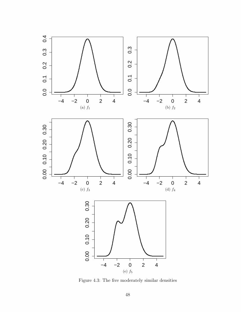
−4 −2 0 2 4
0.0
0.1
0.2
0.3
0.4
(a) f1
−4 −2 0 2 4
0.0
0.1
0.2
0.3
(b) f2
−4 −2 0 2 4
0.00
0.10
0.20
0.30
(c) f3
−4 −2 0 2 4
0.00
0.10
0.20
0.30
(d) f4
−4 −2 0 2 4
0.00
0.10
0.20
0.30
(e) f5
Figure 4.3: The five moderately similar densities
48

Table 4.3: Five Moderately Similar Densities in Ker and Ergün (2005)
f Density Formulaf1 N(0,1)
f2 0.95N(0,1) + 0.05N(−2,0.52)
f3 0.90N(0,1) + 0.10N(−2,0.52)
f4 0.85N(0,1) + 0.15N(−2,0.52)
f5 0.80N(0,1) + 0.20N(−2,0.52)
talbe 4.3. Figure 4.3 plots the five similar densities. Except the lower tail, these five
densities are of generally similar shape.
In empirical applications, we may have a general idea that the true densities
are of similar structure, but the extent of similarity is rarely known. Of course, the
more similar the true densities, the greater efficiency gain can be expected when the
samples are pooled together. The increased sample size contains more information.
With more information, it is more likely to get a better estimation of the underlying
true densities. This is obvious in the best scenario where the true densities are
identical. When the true densities are very dissimilar, like in the first scenario, one
wouldn’t attempt to pool them together. The moderately similar densities represent
the scenario between these two extremes. More often, we only have knowledge that
the true density are possibly similar with unknown extent of similarity. Therefore, the
estimators which have superior performance in this scenario will have great potential
in empirical applications. That is, if one estimator has a greater efficiency gain
compare to others in this scenario, it is very likely that this estimator will outperform
others in the empirical application.
The simulation results of the moderate scenario are shown in table 4.4. Once
again, the two proposed estimators perform exceedingly well. Both Comb1 and
Comb2 outperform KDE, EBayes, Cond, Jones and KerPS in almost all the cases
49

Table 4.4: MISE×1000 for Moderately Similar True Densities, Bandwidths from Min-imizing MISE
n f KDE EBayes Cond KerPS Jones Comb1 Comb2n=25 f1 12.29 12.12 7.99 5.24 7.58 3.62 3.62
f2 11.51 11.22 5.31 3.60 7.11 1.86 2.20f3 11.25 10.89 3.40 2.59 7.57 1.72 1.63f4 11.56 11.10 3.56 3.35 8.23 2.79 2.59f5 11.42 11.00 5.28 5.70 8.65 4.53 4.33
AVG. 11.60 11.26 5.11 4.10 7.83 2.90 2.87
n=50 f1 8.49 8.45 5.49 2.71 4.64 1.57 1.66f2 7.41 7.31 3.53 2.39 4.45 1.20 1.36f3 7.34 7.21 2.14 1.72 4.69 1.27 1.12f4 7.93 7.78 2.58 2.61 5.70 2.17 2.03f5 7.97 7.84 4.34 5.36 6.43 3.93 3.64
AVG. 7.83 7.72 3.61 2.96 5.18 2.03 1.96
n=100 f1 5.05 5.04 4.26 2.87 2.52 1.42 1.69f2 4.87 4.84 2.76 1.65 2.72 0.79 0.93f3 5.01 4.97 1.49 1.20 3.22 0.94 0.81f4 5.01 4.97 1.90 2.18 3.81 1.76 1.61f5 5.00 4.96 3.12 4.85 4.37 3.06 2.62
AVG. 4.99 4.95 2.70 2.55 3.33 1.60 1.53
n=500 f1 1.43 1.43 1.41 1.56 0.51 0.39 0.55f2 1.41 1.41 1.20 0.65 0.73 0.25 0.32f3 1.51 1.51 0.34 0.31 1.02 0.28 0.23f4 1.53 1.53 0.99 1.77 1.15 0.97 0.77f5 1.93 1.93 1.76 1.83 1.99 1.71 1.49
AVG. 1.56 1.56 1.14 1.22 1.08 0.72 0.67
50

except f1 when n=500, where the MISE of Jones is 0.51, lower than 0.55, the MISE
of Comb2. The results are invariant with the sample size changing from 25 to 500. Re-
gardless of the density shape, proposed Comb1 and Comb2 always yield lower MISE.
Comb1 and Comb2 yield the most significant efficiency improvement comparing to
KDE. This is because both Comb1 and Comb2 have bias reduction and variance re-
duction capability while KDE has none. When comparing to KDE, Comb1 reduces
the MISE by 68% , while Comb2 by 71% on average. The maximum efficiency gain
appears on f3 for both Comb1 and Comb2 when the sample size is 25; Comb1 reduces
MISE of KDE from 11.25 to 1.72 by 85% while Comb2 to 1.63 by 88%. Of course, the
efficiency improvement reduces as the sample size increases; with large sample size,
KDE estimates the densities relatively well even without bias and variance reduction
capacity. The least efficiency gain appears on f5 when sample size is 500; Comb1
reduces MISE from 1.93 to 1.71 by 11% while Comb2 by 23%.
Comparing to the best of KDE, EBayes, Cond, Jones and KerPS, Comb1 still
reduces MISE by 27% on average and Comb2 by 29%. This demonstrates the ca-
pability of estimators that reduce both bias and variance. Another observation is
that whenever Jones performs the best among Cond, Jones and KerPS, Comb1 out-
performs Comb2; whenever Cond performs the best among Cond, Jones and KerPS,
Comb2 outperforms Comb1. For example, when n=100, the MISE×1000 of f1 by
Jones is 2.52, the smallest among KDE, Cond, Jones and KerPS. Correspondingly,
Comb1 with MISE×1000 of 1.42 outperforms Comb2 with MISE×1000 of 1.69. When
n=25, the MISE×1000 of f5 by Cond is 5.28, the smallest among KDE, Cond, Jones
and KerPS. Correspondingly, Comb2 with MISE×1000 of 5.33 outperforms Comb1
with MISE×1000 of 4.53. Recall that Comb1 can converge back to Jones but Comb2
can not, similarly Comb2 can converge back to Cond but Comb1 can not. There-
fore, it is likely that when Jones performs the best among Cond, Jones and KerPS,
Comb1 outperforms Comb2. Conversely, wherever Cond performs the best among
51

Table 4.5: MISE×1000 for Identical True Density, Bandwidths fromMinimizing MISE
n KDE EBayes Cond KerPS Jones Comb1 Comb225 13.34 12.64 2.62 1.98 8.29 1.52 0.8550 8.50 8.25 1.49 1.12 4.60 0.76 0.41100 4.97 4.90 0.95 0.74 2.42 0.45 0.23500 1.36 1.36 0.24 0.19 0.55 0.10 0.04
Cond, Jones and KerPS, Comb2 will be more likely to outperform Comb1.
In this moderate scenario, simulation results strongly suggest that the two pro-
posed estimators have superior performance. Comparing to KDE, EBayes, Cond and
KerPS, the two proposed estimators stand out with no obvious peers.
4.2.3 Identical
Finally, I present the scenario where all the densities are exactly the same (or per-
fectly similar). To this end, I assume the nine densities are all standard Gaussian. It’s
logical to pool all the samples together to estimate the density in this case. There-
fore, I expect great efficiency gain when the proposed methods are used to “borrow”
information from other samples.
The simulated results of the best scenario are shown in table 4.5. Again, the
performance of the two proposed estimators is exceptionally well. Comb1 and Comb2
outperform all other competing estimators. Comparing to KDE, Comb1 reduces the
MISE by 91% on average while Comb2 by 95%. Similar magnitude of efficiency
improvement can also be found when comparing to EBayes and Jones. Comparing
to EBayes, MISE is reduced by 91% in Comb1 and 95 % in Comb2. As for Jones,
MISE is reduced by 82% in Comb1 and 91 % in Comb2.
Cond and KerPS are aleady reasonably well performing estimators. However,
even comparing to these two, the proposed estimators can reduce the MISE signifi-
cantly. On average, Comb1 is able to reduce MISE by 50% when comparing to Cond,
52

while Comb2, even better, by 75%. When comparing to KerPS, Comb1 reduces the
MISE by 36% on average, with the minimum of 23% and maximum of 48%. Comb2,
more impressively, reduces the MISE by 67% on average, with the minimum of 57%
and maximum of 78%.
4.3 True Densities Are Unknown
In empirical application, one can not use the minimization of MISE to select band-
widths as the true densities are rarely, if ever, known. Instead, as discussed in section
2.3.1, one can use rule-of-thumb and plug-in method, least squares cross-validation
or maximum likelihood cross-validation. The maximum likelihood cross-validation
method is used to select bandwidth in this research as it is both intuitive and easy to
implement. To clarify, the true densities are obviously known to calculate ISE but are
considered unknown during the bandwidth selecting process. That is, the maximum
likelihood cross-validation method is used to select the optimal bandwidths. These
bandwidths are then used to calculate the estimated densities. Then the ISE between
estimated densities and true densities are calculated to measure the efficiency of the
estimator. EBayes estimator is not included in this part as it is explored in detail in
Ramadan (2011).
In KDE, the bandwidth is selected in
maxhL1 = lnL1 =
n∑i=1
lnfKDE−i (Xi;h), (4.6)
where −i indicates leaving sample i out. fKDE(Xi;h) is the estimated density at
sample point Xi with KDE estimator. n is the sample size of the individual sample.
53
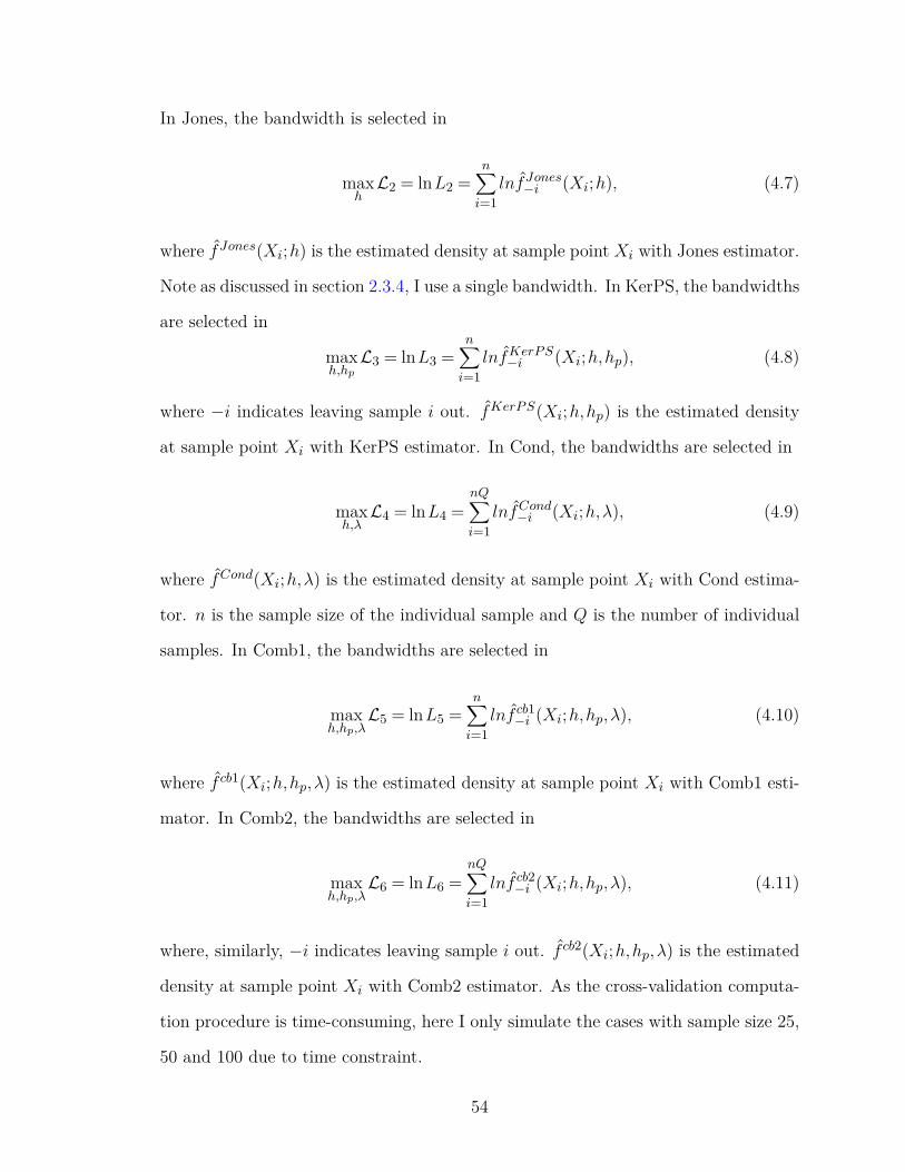
In Jones, the bandwidth is selected in
maxhL2 = lnL2 =
n∑i=1
lnfJones−i (Xi;h), (4.7)
where fJones(Xi;h) is the estimated density at sample point Xi with Jones estimator.
Note as discussed in section 2.3.4, I use a single bandwidth. In KerPS, the bandwidths
are selected in
maxh,hp
L3 = lnL3 =n∑i=1
lnfKerPS−i (Xi;h,hp), (4.8)
where −i indicates leaving sample i out. fKerPS(Xi;h,hp) is the estimated density
at sample point Xi with KerPS estimator. In Cond, the bandwidths are selected in
maxh,λL4 = lnL4 =
nQ∑i=1
lnfCond−i (Xi;h,λ), (4.9)
where fCond(Xi;h,λ) is the estimated density at sample point Xi with Cond estima-
tor. n is the sample size of the individual sample and Q is the number of individual
samples. In Comb1, the bandwidths are selected in
maxh,hp,λ
L5 = lnL5 =n∑i=1
lnf cb1−i (Xi;h,hp,λ), (4.10)
where f cb1(Xi;h,hp,λ) is the estimated density at sample point Xi with Comb1 esti-
mator. In Comb2, the bandwidths are selected in
maxh,hp,λ
L6 = lnL6 =nQ∑i=1
lnf cb2−i (Xi;h,hp,λ), (4.11)
where, similarly, −i indicates leaving sample i out. f cb2(Xi;h,hp,λ) is the estimated
density at sample point Xi with Comb2 estimator. As the cross-validation computa-
tion procedure is time-consuming, here I only simulate the cases with sample size 25,
50 and 100 due to time constraint.
54
4.3.1 Low Similarity
Again, the nine dissimilar densities are used to represent the low similarity scenario.
The results are reported in table 4.6. As expected, comparing to the previous case
where the true densities are known, the MISE from cross-validation is larger. The
highest MISE is from f5. This is understandable. Recall that f5 is the outlier density
in Marron and Wand (1992) with a spike around 0. Using the other n− 1 points to
estimate the density of Xi would be difficult, especially for Xi near 0. The reason is
that to better estimate f5 around the thin region near 0, a small bandwidth is required,
but for all other region away from 0, a large bandwidth is required. It’s hard to find
a single bandwidth that performs well over the entire domain by cross-validation. f3
and f4 have large MISE for similar reason. To select a reasonable bandwidth for these
three less smooth densities, too small bandwidth should be avoided as suggested by
Hall, Racine, and Li (2004). When searching the optimal bandwidths for f3, f4 and
f5, the second smallest local minimum is selected rather than the smallest.
Comparing the performance of Comb1 and Comb2, except f5 when n is 25 and
f3 when n is 100, Comb1 dominates Comb2 in estimating f3, f4 and f5. This might
relates to the fact that Comb1 can converge back to Jones but not Comb2. In these
three relatively rough densities, Jones performs really well. By converging towards
Jones, Comb1 can also perform well in estimating f3, f4 and f5.
On average, KDE has the largest MISE. The MISE of Cond and KerPS are close
to KDE’s. Among KDE, Cond, Jones and KerPS, Jones performs the best on average.
This is reasonable as Jones only utilizes information from its own experiment unit.
The nine densities are very dissimilar, borrowing information from other experiment
units can hardly help to improve the estimation efficiency in this case. Except when
sample size is 100 where Jones has a lower MISE than Comb1. On average, Comb1
outperforms its three special cases, KDE, Jones and KerPS. Comb2 also outperforms
55

Table 4.6: MISE×1000 for Dissimilar True Densities, Bandwidths from Cross-Validation
n f KDE Cond Jones KerPS Comb1 Comb225 f1 20.83 20.92 25.97 19.94 19.24 14.90
f2 30.41 28.79 33.84 26.54 28.92 33.99f3 155.55 151.72 142.07 155.79 143.55 156.06f4 197.57 196.43 173.17 191.99 173.04 201.03f5 721.82 715.35 526.54 723.24 515.39 483.90f6 24.59 26.58 33.09 24.36 24.98 25.65f7 37.76 37.92 45.55 38.21 36.32 41.92f8 28.72 28.26 37.78 28.48 27.83 31.18f9 28.04 28.40 35.06 30.17 28.59 31.32
AVG. 138.37 137.15 117.01 137.64 110.87 113.33
50 f1 11.65 11.74 14.78 10.80 11.98 7.69f2 17.65 16.12 17.34 16.95 14.95 21.42f3 112.56 108.93 99.07 114.79 95.70 104.06f4 154.39 149.30 132.98 148.24 132.75 152.48f5 611.15 572.77 381.93 604.84 382.55 551.07f6 15.01 16.08 19.73 15.03 14.47 19.93f7 22.00 21.85 25.25 21.33 22.36 24.16f8 17.81 17.93 22.74 18.10 17.39 21.11f9 17.10 17.62 21.59 17.23 17.22 22.33
AVG. 108.81 103.59 81.71 107.48 78.82 102.69
100 f1 7.16 7.64 8.62 6.61 7.00 5.78f2 10.37 10.38 9.59 9.54 9.07 14.48f3 77.79 76.17 66.59 78.22 67.83 64.94f4 111.87 108.00 85.75 108.29 89.80 92.69f5 439.40 410.67 178.93 445.25 272.92 370.68f6 9.11 9.65 11.79 8.84 9.56 11.52f7 12.70 12.83 14.25 12.97 12.66 13.77f8 11.34 11.30 12.93 11.10 11.42 14.80f9 10.54 10.67 13.07 10.31 10.83 12.62
AVG. 76.70 73.04 44.61 76.79 54.56 66.81
56

its three special cases KDE, Cond and KerPS on average across all three sample sizes.
The maximum likelihood cross-validation method performs better when the
underlying true densities are smooth. Relatively rough densities f3, f4 and f5 have
larger MISE comparing to the other six densities. Also notice the MISE of f5>f4>f3.
This is because f5 has the most rough density shape, f4 stays in the middle in terms
of roughness while the right-hand side of f3 is relatively smooth. Comparing the
MISE of f6 and f9, the maximum likelihood cross-validation method performs better
when the true densities have less models. The maximum likelihood cross-validation
method also performs better when the underlying true densities are symmetric; the
symmetric f1 has smaller MISE comparing to left-skewed f2 and the symmetric f6
has smaller MISE comparing to asymmetric f8. The MISE of f6 is smaller than f7.
Although they are both bi-model, f6 is smoother than f7. As a result, cross-validation
method tends to perform better in selecting bandwidths for f6 than f7.
4.3.2 Moderate Similarity
For the moderate similarity scenario, the results are represented in table 4.7. Comb2
performs the best on average followed by Cond, KerPS and KDE. Jones performs the
worst. The MISE of Comb2 is 24% (22% and 23%) smaller than that of KDE when n is
25 (50 and 100). Cond reduces the MISE by 9% (5% and 10%) comparing KDE when
n is 25 (50 and 100). Similarly, the MISE of KerPS is 9% (5% and 5%) smaller than
that of KDE when n is 25 (50 and 100). Comb1 has smaller MISE comparing to KDE
when n is 25 and 50, but not 100. Recall that Comb1 can theoritically converge back
to KerPS, Jones and KDE. Notice also that Jones has the highest MISE on average
for all three sample sizes. This may seem suprising since Jones performs relatively
well in the low similarity scenario. Further examination reveals that Jones performs
well in estimating f3, f4 and f5 in the low similarity scenario, but not for the other
6 realatively smoother densities. f3, f4 and f5 share a similar characteristic: a sharp
57

Table 4.7: MISE×1000 for Moderately Similar True Densities, Bandwidths fromCross-Validation
f KDE Cond Jones KerPS Comb1 Comb2n=25 f1 21.93 19.69 27.90 17.82 18.80 16.37
f2 20.42 14.83 24.10 18.03 18.98 15.00f3 19.92 23.93 24.74 19.08 19.40 14.44f4 20.10 16.84 25.08 18.50 17.49 15.93f5 22.34 20.00 26.56 21.85 21.50 17.46
AVG. 20.94 19.06 25.68 19.06 19.23 15.84
n=50 f1 11.92 11.05 14.40 10.90 10.67 10.02f2 11.61 10.38 14.46 10.85 11.36 9.31f3 11.93 10.33 15.25 11.43 11.57 7.02f4 11.82 11.72 15.73 11.68 11.76 8.62f5 11.78 11.13 15.93 11.38 12.19 11.22
AVG. 11.81 10.92 15.15 11.25 11.51 9.24
n=100 f1 7.58 6.82 8.35 7.27 7.30 6.47f2 6.81 6.21 8.71 6.59 7.20 5.04f3 7.10 5.96 9.63 6.78 7.16 4.81f4 7.24 6.35 9.29 6.75 7.55 5.22f5 7.64 7.57 10.14 7.29 7.43 6.51
AVG. 7.27 6.58 9.23 6.94 7.33 5.61
58

peak. This indicates that Jones may perform better in estimating realatively rough
densities than smooth densities. The five possibly similar densities are all realatively
smooth so Jones’ performance may not be that suprising. As shown in figure 3.2, in
order to converge back to KDE, the bandwidth in Jones hJ should be equal to h, the
bandwidth in KDE, and hJp should be infinity. But in the cross validation case, I
followed Jones, Linton, and Nielsen (1995) and set hJ = hJp. As a result, it is very
hard for Jones to converge back to KDE. This might explain why Jones performs
worse than KDE.
Comb2 outperforms Comb1 in all simulations. On average, the MISE from
Comb2 is 20% smaller than Comb1. Comparing KDE, Cond, Jones and KerPS, Cond
performs the best; it yields the lowest MISE regardless of the density shape and sample
size. Hall, Racine, and Li (2004) showed that cross-validation in Cond can effectively
reduce variance. Here all the five densities are similar in shape, the estimators may
have small bias but relatively large variance. Thus bias reduction methods may not
improve efficiency as significant as variance reduction methods. This might explain
why Comb2 outperforms Comb1; although both Comb1 and Comb2 have the ability
to reduce bias and variance, Comb1 might work better at reducing bias while Comb2
better at reducing variance.
4.3.3 Identical
Finally, the simulation results for the identical scenario where all five true densities
are standard Gaussian are presented in table 4.8. As the five densities are identical,
Table 4.8: MISE×1000 for Identical True Density, Bandwidths from Cross-Validation
n KDE Cond Jones KerPS Comb1 Comb225 21.86 18.71 25.58 19.28 18.42 15.7450 12.30 10.77 15.08 11.03 12.00 7.93100 7.12 5.92 8.57 6.47 7.36 4.28
59

only the average MISE of each method for each sample size is reported. Comparing
KDE, Cond, Jones and KerPS, Cond has the smallest MISE across all three sample
sizes. Comb1 outperforms KDE, Cond, Jones and KerPS when sample size is 25.
But when sample size increases to 50 and 100, KerPS and Cond start to outperform
Comb1. When n is 100, Comb1 only outperforms Jones. Comb2 consistently yields
lower MISE regardless of the sample size. When n is 25, the MISE of Comb2 is 28%
smaller than that of KDE. As n increases, the advantage is more obvious: 36% smaller
than KDE when n is 50 and 40% when n is 100.
The performance of Jones, similar to the previous case, is the worst comparing to
other methods. This again indicates that using only one bandwidth in Jones may not
provide efficiency gain if the underline true densities are smooth. KerPS, pooling all
the data from the same true density together to form a start, reduces MISE by 10% on
average comparing to KDE. When the five true densities are identical, the estimated
densities may have smaller bias and larger variance. This could then explain why the
variance reduction Cond performs better than bias reduction Jones and KerPS.
4.4 Summary
This chapter tests the performance of the two proposed estimators by simulations.
The performance is measured by integrated squared error. The simulation is designed
to represent two scenarios: true densities are known where bandwidths are selected by
minimizing mean integrated squared error and true densities are assumed unknown
where bandwidths are selected by maximum likelihood cross-validation. Each scenario
contains three cases: the best case where the true densities are identical; the moderate
case where the true densities are moderately similar and the worst case where the
true densities are dissimilar. The optimal bandwidth from KerPS and Cond are used
as the starting value for Comb1 and Comb2 to potentially reduce computation time.
60

The density estimators which do not integrate to 1 are renormalized to be able to
integrate to 1. The density transformation method from Ker (2014) is applied in
KerPS, Comb1 and Comb2.
The simulation results confirm that Comb1 and Comb2 outperforms its spe-
cial cases when the bandwidths are selected by minimizing integrated squared error.
When the true densities are assumed to be unknown and the bandwidths are se-
lected by maximum likelihood cross-validation, Comb1 performs relatively well when
the true densities are dissimilar. Comb2 outperform other methods when the true
densities are moderately similar or identical.
61

Chapter 5
Application
To evaluate the empirical performance of the two proposed estimators, I apply them
to estimate crop yield densities. Their performance are then compared to other
alternatives: KDE, Jones, KerPS, Cond, and the empirical method currently adopted
by RMA. This case study, like most empirical settings where we do not have enough
knowledge of the form or extent of similarities of the underline true densities, is an
ideal situation to demonstrate the strength of the proposed estimators. This chapter
presents the data, some empirical considerations, design of the insurance policies
rating game, the results and conclusions.
5.1 Data
The data used in this application is county-level yields for corn and soybean in Illinois
from 1955 to 2013. Data are from the National Agricultural Statistics Service (NASS)
online database. Illinois is selected not only because it is one of the major corn
producers, accounting for 15.6% of national corn production, but also because it is
one of the area where the majority of GRP and GRIP policies are sold. A case study
of Illinois corn has implication relevant for the USDA’s area yield crop insurance
program. Although the state of Illinois consists of 102 counties, only 82 are used for
analysis due to missing data. Moreover, the data before 1955 is discarded because of
the dramatic change in crop production and crop genetic advancement. Figure 5.1
shows corn yields of four randomly sampled counties.
County-level yield data is used. The advantage of using county-level data is that
62

1960 1970 1980 1990 2000 2010
8010
012
014
016
018
020
0
year
Yiel
d in
Bur
eau
(Bus
hels
/Acr
e)
(a)
1960 1970 1980 1990 2000 201060
8010
012
014
016
018
020
0
year
Yiel
d in
De
Kalb
(Bus
hels
/Acr
e)
(b)
1960 1970 1980 1990 2000 2010
6080
100
120
140
160
180
year
Yiel
d in
Cha
mpa
ign
(Bus
hels
/Acr
e)
(c)
1960 1970 1980 1990 2000 2010
5010
015
0
year
Yiel
d in
Whi
te (B
ushe
ls/A
cre)
(d)
Figure 5.1: County-level average corn yield for four randomly sampled counties, Illi-nois
63

Table 5.1: Summary Statistics of Yield Data, Corn, Illinois, 1955-2013
Counties Min Mean Median Max Std.Dev.CRD1 10 52.0 120.7 119.0 199.6 34.9CRD2 7 49.0 118.0 116.0 197.0 35.5CRD3 9 35.0 117.5 117.0 207.0 37.1CRD4 9 42.0 124.8 124.0 206.0 37.3CRD5 7 42.0 121.3 123.0 191.0 35.6CRD6 11 49.0 118.7 121.0 200.0 36.7CRD7 12 19.0 109.0 110.0 191.0 37.8CRD8 9 21.1 90.5 87.0 181.0 34.7CRD9 8 28.0 93.3 90.0 188.7 35.3
Note: Yields reported in bushels per acre. Data from National Agri-cultural Statistic Service.
CRD 1
CRD 2
CRD 3
CRD 4
CRD 5
CRD 6
CRD 7
CRD 8
CRD 9
Source: National Agricultural Statistics Service, United States Department of Agriculture.
Figure 5.2: Crop reporting districts in Illinois
the effect of moral hazard is mitigated in area-yield insurance programs as discussed
in literature review. There is also more data available on county-level than farm-
level. Arguably, the effect of adverse selection is also reduced on county-level; there is
less private information about the data-generating process of the yield that triggers
indemnities (Ozaki et al., 2008).
The data from each county is grouped by crop reporting district (CRD). The
summary statistics segmented by crop reporting districts are provided in table 5.1.
A map of the study area is shown in figure 5.2.
64

5.2 Empirical Considerations
Some general concerns when working with yield data are discussed in this section,
including spatial correlation, heteroscedasticity, and technological trend.
Spatial Correlation
One can pool extraneous data together with data from the own county to increase
the sample size and improve estimation efficiency. But this is conditional on the ex-
traneous data and own data being independent and from identical distribution. It
is worth-noting that crop reporting districts (CRDs) represent divisions of approxi-
mately equal size with similar soil, growing conditions and types of farms1. Because
yields are highly influenced by weather, soil type and production practices, it is likely
that the yields data within a CRD are spatially correlated. Spatial correlation, vi-
olating the independent requirement, decreases the efficiency gain of the estimators
which utilize information from extraneous counties. Ker (2014) showed that spatial
correlation decreased the estimation efficiency of KerPS. But comparing with pooled
estimator (KDE with all data pooled together), the efficiency of KerPS relative to the
pooled estimator remained constant regardless of the presence of spatial correlation.
Hypothetically, although the presence of spatial correlation reduces the efficiency of
all estimators utilizing extraneous information, the relative performance of Comb1
and Comb2 may not change. Cond, KerPS, Comb1 and Comb2 all perform less effi-
cient when spatial correlation is present, but Comb1 and Comb2 may still outperform
Cond and KerPS. Therefore, the presence of spatial correlation may not alter the main
conclusions. However, due to time constraints, this is not further investigated. Lastly,
if spatial correlation is expected to have great impact, one can always apply blocked
cross-validation to choose the bandwidths.1Illinois Agricultural Statistics, Annual Summary, 1985, Bulletin 85-1
65

Heteroscedasticity
The second concern is the existence of heteroskedasticity. Crop yield variance may
change over time. Recognition of heteroscedasticity in crop yields is critical for proper
estimation of yield densities and premium rates. Failure to correct for heteroscedas-
ticity, if it is present, will lead to inaccurate estimations of yield density and thus
inaccurate estimations of premium rates as pointed out in Ozaki, Goodwin, and Shi-
rota (2008).
Following Harri et al. (2011), this research models yield heteroscedasticity as
a function of the predicted yield. That is var(et), the variance of error term, is a
function of fitted-value yt and heteroscedasticity coefficient β as follow:
var(et) = σ2ytβ. (5.1)
Note β = 0 indicates homoscedastic errors. β = 1 indicates the variance of the error
term moves in direct proportion to the predicted yield. And β = 2 indicates the
standard deviation of the error term moves in proportion to the predicted yield.
The heteroscedasticity coefficient β is estimated in
ln et2 = α+β ln yt+ εt, (5.2)
where εt is a well-behaved error-term. Following Tolhurst and Ker (2015), the es-
timated β is restricted to be between 0 and 2; β larger than 2 is restricted to be
2.
Trend
As a result of technological advances in seed development and farm practice, crop
yields data normally has an upward trend. To use historical yield data to estimate
66

current losses, it is necessary to remove the trend effect of technology. The trend
of crop yields can be modeled in several ways. Parametric methods include methods
such as the linear trend, one-knot linear spline model and two-knot linear spline model
currently adopted by RMA. Vedenov, Epperson, and Barnett (2006) examined the
three- and four- knot spline trend function and found no significant improvement.
Tolhurst and Ker (2015) used a mixture model which estimated two trend lines each
for a subpopulation of yields. One can also use nonparametric methods to model the
technical trend.
I adopt RMA’s current trend estimation method. It is a two-knot linear spline
model with robust M-estimation2. The two-knot linear spline model is defined as
yt = γ1 +γ2t+γ3d1(t−knot1) +γ4d2(t−knot2) + et (5.3)
d1 = 1 if t≥ knot1, 0 otherwise,
d2 = 1 if t≥ knot2, 0 otherwise.
Following Harri et al. (2011), I also iterate using Huber weights until convergence and
then use Bisquare weights for two iterations. Huber weights wH(e,c) is
wH(e,c) =
1 if |e|< c
c
|e|if |e| ≥ c,
(5.4)
2Robust regression can be used in any situation in which one would use least squares regression.When fitting a least squares regression, we might find some outliers or high leverage data points.We have decided that these data points are not data entry errors, neither they are from a differentpopulation than most of our data. So we have no compelling reason to exclude them from theanalysis. Robust regression might be a good strategy since it is a compromise between excludingthese points entirely from the analysis and including all the data points and treating all them equallyin OLS regression. The idea of robust regression is to weigh the observations differently based onhow well behaved these observations are. Roughly speaking, it is a form of weighted and reweightedleast squares regression.
67

where c has the defult value of 1.345. And Bisqure weights wB(e,c) is
wB(e,c) =
(
1−(ec
)2)2if |e|< c
0 if |e| ≥ c,(5.5)
where c has the defult value of 4.685.
To increase the stability of the estimated trend over time and across space,
RMA imposes temporal and spatial prior restrictions on the knots for the spline
models. However, after imposing temporal restriction, I found the trend is already
fairly stable in my study area, thus spatial prior is not applied here. The reason
is that more restrictions force the estimated trend further away from its optimal
position. As long as the estimated trend is fairly stable, less prior restriction should
be imposed. Representative trend estimations are displayed in figure 5.3. There are
lots of technical trend lines each with different data length. For example, the 1955-
2012 data is used to estimate one trend line, the 1955-2011 data is used to estimate
another, the 1955-2010 data forms the third trend line. All these trend lines are
plotted together in each panel. Generally speaking, the estimated two-knot linear
spline trends are stable over time. Especially in panel (b) and (c) where most of the
estimated trend lines overlap although they are estimated with different data length.
The trend lines diverge at the most recent years. This is because the 2012 yields are
dramatically lower than previous years due to very dry late season and severe storms
earlier in the growing season. As a result, estimated trends with and without 2012
data are different.
68

Yiel
d (B
ushe
ls p
er A
cre)
1960 1970 1980 1990 2000 2010
5010
015
020
0
(a) Corn yield, Adams, Illinois
1960 1970 1980 1990 2000 2010
5010
015
020
0Yi
eld
(Bus
hels
per
Acr
e)
(b) Corn yield, Brown, Illinois
1960 1970 1980 1990 2000 2010
5010
015
020
025
0Yi
eld
(Bus
hels
per
Acr
e)
(c) Corn yield, Carroll, Illinois
1960 1970 1980 1990 2000 2010
100
150
200
250
Yiel
d(B
ushe
ls p
er A
cre)
(d) Corn yield, Champaign, Illinois
Figure 5.3: The estimated two-knot spline trend in representative counties
69

The estimated heteroscedasticity coefficient β (from 5.2), together with the
predicted yield yT+1 (from 5.3) using two-knot linear spline model, are then used to
derive heteroscedasticity corrected and detrend yields yt as
yt = yT+1 + etyβT+1
yβt
. (5.6)
yt, the detrend and heteroscedasticity corrected yield data is used to estimate yield
density in the later out-of-sample simulation game. The adjusted yields are shown in
figure 5.4 for some randomly selected counties over different time periods.
For relatively large sample size, the optimization process in the proposed es-
timators will take a longer period of time. The reason is that both Comb1 and
Comb2 need to choose three parameters. To speed up the optimization process, op-
timal bandwidths from KerPS and Cond are used as starting values in Comb1 and
Comb2. The intuition is that KerPS or Cond estimator is treated as starting point
from which Comb1 and Comb2 continue to improve the estimation efficiency. Rep-
resentative estimated densities by different methods are shown in figure 5.6 and 5.7
for four randomly selected counties in Illinois. KDE performs most differently than
other estimators with fatter lower tail. The densities estimated by Comb1 are close
to the one estimated by KerPS, indicating that Comb1 hardly improves estimation
efficiency upon KerPS. On the lower tail, KerPS and Comb1 are more likely to cap-
ture the effect of lower yields (see panel a, b and c); their densities are more likely to
have a small bump on the lower tail. Comparing to KerPS and Comb1, Cond tends
to estimate smaller density values on the lower tail and larger density values on the
upper tail. On the lower tails where KerPS and Comb1 estimate a small bump, Cond
tends to be more smooth with no bump. The densities estimated by Comb2 are close
to the ones estimated by Cond, but generally, the density curves of Comb2 are more
smooth with almost no bumps. For example, when using 1955-2009 yields data to
70

1960 1970 1980 1990 2000
5010
015
020
0
Year
Yiel
ds a
nd A
djus
ted
Yiel
ds
(a) Carroll 1955-2000
1960 1970 1980 1990 2000 2010
100
150
200
250
YearYi
elds
and
Adj
uste
d Yi
elds
(b) Christian 1955-2011
1960 1970 1980 1990
6080
100
120
140
160
180
Year
Yiel
ds a
nd A
djus
ted
Yiel
ds
(c) Coles 1955-1993
1960 1970 1980 1990
6080
100
120
140
160
Year
Yiel
ds a
nd A
djus
ted
Yiel
ds
(d) Cumberland 1955-1996
Figure 5.4: Detrend and hetroscedasticity corrected yield
Note: Black squares are the original data, lines are estimated trend and red circles are adjustedyield.
71

0 100 200 300 400 500 600 700
0.00
00.
005
0.01
00.
015
Grid
Den
sity
f.kdef.condf.Jonesf.Kpsimf.cb1f.cb2
Figure 5.5: Estimated corn yiled densities in Henry, Illinois with 1955-2009 data
estimate corn yield density in Henry, Illinois, Cond estimates two small bumps on the
lower tail while Comb2 smoothes them out (see figure 5.5). This might be because
that comparing to variance-reducing Cond, Comb2 reduces both variance and bias,
resulting smoother estimated density.
72

0 200 400 600 800
0.00
00.
002
0.00
40.
006
0.00
80.
010
0.01
20.
014
1955− 2006 Corn Yield Density Estimation in bureau Illinois
Grid
Den
sity
(a) (b)
0 200 400 600 800
0.00
00.
005
0.01
00.
015
0.02
0
1955− 2007 Corn Yield Density Estimation in mercer Illinois
Grid
Den
sity
f.kdef.condf.Jonesf.Kpsimf.cb1f.cb2
(c) (d)
Note: The left panels plot the entire estimated densities, the corresponding panels on the right showthe enlarged lower tail.
Figure 5.6: Estimated densities from different methods (1/2)
73

0 200 400 600 800
0.00
00.
005
0.01
00.
015
1955− 2007 Corn Yield Density Estimation in whiteside Illinois
Grid
Den
sity
f.kdef.condf.Jonesf.Kpsimf.cb1f.cb2
(a) (b)
0 200 400 600
0.00
00.
002
0.00
40.
006
0.00
8
1955− 2008 Corn Yield Density Estimation in jo daviess Illinois
Grid
Den
sity
f.kdef.condf.Jonesf.Kpsimf.cb1f.cb2
(c) (d)
Note: The left panels plot the entire estimated densities, the corresponding panels on the right showthe enlarged lower tail.
Figure 5.7: Estimated densities from different methods (2/2)
74

5.3 Design of the Game
Fair Premium
Define y as the random variable of average yield in an area, λye as the guaranteed
yield where 0 ≤ λ ≤ 1 is the coverage level and ye is the predicted yield, fy(y|It)
is the density function of the yield conditional on information available at time t.
An actuarially fair premium, π, is equal to the expected indemnity as shown in the
following equation:
π = P (y < λye)(λye−E(y|y < λye)) =∫ λye
0(λye−y)fy(y|It)dy. (5.7)
Note It is the information set known at year t, the time of rating insurance contracts.
In the analysis that follows, the information set It includes past county-level yield
data (from year 1955 to t−1) and the county in which they were recorded. Note also
that the premium defined here is in terms of crop yield with bushels per acre as the
units.
The Adverse Selection Game
As commonly done in the literature (Ker and McGowan, 2000; Ker and Coble, 2003;
Racine and Ker, 2006; Harri et al., 2011; Tolhurst and Ker, 2015), the simulated
contract rating game is designed as follows. There are two agents in the out-of-
sample simulation game: (i) the private insurance company(IC), which is assumed to
derive rates from one of the two proposed density estimation methods, and (ii) the
RMA which is assumed to derive rates from one of the other methods (i.e., Standard
Kernel Density Estimator (KDE), Conditional Density Estimator (Cond), Jones’ Bias
Reduction Method (Jones), Ker’s Possibly Similar estimator (KerPS), and Empirical
rating method used by RMA (Empirical)).
75

>
>
Retain Contractsof IC
Contractsof RMA
Actural Realization
Cede
Figure 5.8: The decision rule of private insurance company
Assuming the rating happens at year t, then all information available at that
time is yield data up to year t−1 and the county where it is recorded. The game is
repeated for 20 years with year t = 2013, 2012, · · · , 1994. That is, to calculate the
premium for year t, data from 1955 to t− 1 is used. For example, when calculating
pseudo premium for both the private insurance company and the government (or
RMA) at year 2013, I use all data from 1955 to 2012. Similarly, to calculate premium
rate for year 2012, data from 1955 to 2011 is used.
The simulation imitates the decision rule of the Standard Reinsurance Agree-
ment where private insurance company can adversely select against the RMA ex ente
as illustrated in figure 5.8. At year t, with data from 1955 to t−1 in all Q counties in
CRD k, the private insurance company uses Comb1 (or Comb2) to estimate its pre-
mium rate for county q at year t as ΠqtIC . The RMA, with the same data, uses one of
the five methods (Empirical, KDE, Jones, KerPS and Cond) to estimate its premium
rate for the same county at the same year as ΠqtRMA. The private insurance company
retains policies with rates lower than the RMA rates (ΠqtIC < Πqt
RMA) because ex ante
76

it expects to earn a profit on those policies. Conversely, the insurance company will
cede policies when it thinks the policies are underpriced (ΠqtIC > Πqt
RMA).
After this selecting process, the entire policy set of size 1740 (82 counties × 20
years) will be divided into two sets: one retained by the insurance company, set F ;
one ceded by insurance comany and therefore retaind by RMA , set F c. The loss
ratio of each set is calculated using actual yield realizations from 1993 to 2013. For
example, the loss ratio for the insurance company (i.e. set F ) is
Loss RatioF =∑j∈F max(0,λyej −yj)wj∑
j∈F ΠjRMAwj
, (5.8)
where wj is the weight assigned to the county-level results; it aggregates the loss
ratio to state level3. Note the premiums received by the insurance company in the
denominator is ΠRMA, not ΠIC . Because the price of the policies is set by RMA. The
retain or cede decision is at county level. Results are then aggregated to state level
as commonly done in the literature. Randomization methods are used to calculate p-
value with 1000 randomizations. For example, by adopting a new density estimation
method, the private insurance company adversely selected 40% of all the contracts
and its loss ratio is 0.8. The p-value is calculated as follows. First, 40% of the
contracts are randomly selected from the entire contract pool and its loss ratio LR1
is calculated. Second, step 1 is repeated for 1000 times generating 1000 loss ratios
LR1, LR1, · · · , LR1000. The p-value is the percentage of loss ratios among these 1000
that are lower than the insurance company’s loss ratio (0.8).3This weight is based on the share of corn production of that county in its state in terms of
planting acreage.
77
5.4 Results
The simulation results with corn data from Illinois are shown in table 5.2. The results
where private insurance company is assumed to derive rates using Comb1 is reported
on the top of the table while the bottom is results using Comb2. Comb1 significantly
outperforms the RMA’s current method, KDE and Jones all with p-value less than
0.05. When comparing to KerPS, the insurance company still gets lower loss ratio
by adopting Comb1, but the advantage is no longer statistically significant. Comb1
fails to outperform Cond and Comb2. Instead, when the private insurance company
derives its rates using Comb2, significant rents can be garnered if the government
derive its rates by the empirical method, Jones, KerPS or Comb1. Comb2 does insure
the private insurance company to obtain lower loss ratio when the government uses
KDE or Cond, but this result is not statistically significant. Comb2 performs better
than Comb1 enabling the private insurance company to get statistically significant
lower loss ratio. Notice Comb1 can not outperform Cond while Comb2 outperforms
Cond with a p-value of 0.10. Recall that Comb1 can converge back to KDE, Jones
and KerPS, but not Cond; but Comb2 is capable of converging back to Cond. The
performance difference between Comb1 and Comb2 may come from the conditional-
density-component in Comb2.
The percentage of policies retained by the insurance company is around 50%.
This is reasonable given the small differences among the densities estimated by dif-
ferent methods (see figure 5.6 and 5.7 ). How could such similar densities result in
totally different loss ratio? The answer locates on the lower-tail: two densities may
look alike in general, but their lower-tail may differ dramatically. Recall from section
5.3, when calculating the premium rate, only the lower-tail of the density is used.
Therefore, the more dissimilar the lower-tail, the more different the calculated pre-
mium and thus loss ratio. Referring back to figure 5.6 and 5.7 again, we can see in
78

panel (c,d) in figure 5.6 and (a,b) in figure 5.7, the lower-tail of densities estimated by
KerPS and Comb2 differ significantly: KerPS has a bump, whereas Comb2 is more
smooth. It’s then understandable that Comb2 performs differently than KerPS.
Table 5.2: Out-of-sample Contracts Rating Game Results: Corn, Illinois
Pseudo Loss Ratio % RetainedInsurance by Insurance
Program Company Government Company p-value(1) (2) (3) (4) (5) (6)
Insurance Company uses Comb1Empirical 0.96 0.78 1.20 0.57 0.01
KDE 0.97 0.81 1.35 0.69 0.00Jones 0.96 0.85 1.21 0.68 0.04KerPS 0.95 0.90 1.04 0.59 0.20Cond 0.94 0.97 0.89 0.64 0.68
Comb2 0.89 1.04 0.70 0.50 0.98
Insurance Company uses Comb2Empirical 0.91 0.63 1.16 0.44 0.00
KDE 0.92 0.80 0.99 0.32 0.15Jones 0.91 0.69 1.10 0.45 0.01KerPS 0.90 0.67 1.05 0.40 0.01Cond 0.89 0.80 1.01 0.58 0.10
Comb1 0.90 0.70 1.05 0.44 0.02
Note: Column (1) is the pseudo rating methods adopted by the government.
The results with soybean data from Illinois are presented in table 5.3. Comb2
can obtain lower loss ratio comparing to the six alternative methods used by the
government. Insurance company’s loss ratio is only 41% of government’s on average,
with a minimum of 34% and a maximum of 51%. That is, on average, Comb2 is
capable of reducing loss ratio by 33.5%. This advantage is also statistically significant:
5 out of 6 have p−value less than 5%. Comb1 yields statistically significant lower loss
ratio when the government rating method is the empirical or Jones. Comb1 performs
similarly as KDE and KerPS where the private insurance company’s loss ratio is
similar to the government’s. Comb1 can not outperform Cond and Comb2. For the
79

soybean data, Comb2 performs the best comparing to all others, including Comb1.
Recall in figure 5.6 and 5.7, the shape of Comb1 estimators are similar to KerPS and
Comb2 are similar to Cond. When Cond performs better, Comb2 tends to perform
better. Comb1’s performance tends to be associated with the performance of KerPS.
For our data environment with yields of corn and soybean, Cond outperforms KerPS,
as a result, Comb2 outperforms Comb14.
Table 5.3: Out-of-sample Contracts Rating Game Results: Soybean, Illinois
Pseudo Loss Ratio % RetainedInsurance by Insurance
Program Company Government Company p-value(1) (2) (3) (4) (5) (6)
Insurance Company uses Comb1Empirical 1.04 0.85 1.40 0.52 0.02
KDE 1.08 1.06 1.09 0.28 0.47Jones 1.04 0.83 1.45 0.53 0.01KerPS 1.05 1.02 1.07 0.41 0.41Cond 1.04 1.21 0.86 0.50 0.98
Comb2 1.05 1.26 0.83 0.50 0.99
Insurance Company uses Comb2Empirical 1.04 0.76 1.54 0.48 0.00
KDE 1.08 0.85 1.33 0.39 0.04Jones 1.04 0.83 1.39 0.46 0.03KerPS 1.05 0.86 1.30 0.43 0.04Cond 1.04 0.96 1.52 0.80 0.06
Comb1 1.05 0.76 1.40 0.42 0.01
Note: Column (1) is the pseudo rating methods adopted by the government.
4In simulation game where the government uses KerPS and private insurance company uses Cond,the loss ratio for the insurance company is only 0.72 comparing to the government’s 1.13 for cornyields data. This results are also significant with a p-value of 0.01. The detailed results can be foundin Appendix table 1. For soybean data, similarly the private insurance company has loss ratio of0.66 comparing to the government’s 1.09. Details can be found in Appendix table 2.
80

5.5 Sensitivity Analysis
The performance of the two proposed estimators are promising, especially Comb2.
But given the technological advances in seed development, the validity of using the
earlier yield data (1950-70s) in estimating current losses is a concern. On the other
hand, the Supplemental Coverage Option introduced in the 2014 farm bill enables
farmers to buy crop insurance based on county-level yield or revenue. However, some
counties and crops have only limited historical data. It’s worthwhile to investigate
whether the proposed estimators would still perform well with small sample. The
main results in the empirical game use historical yield data starting from 1955. This
section analyzes how the main results change as only the most recent yield data
is used. To be more specific, instead of using yield data from 1955 to the year of
analysis, here only the most recent 25 or 15 years of yield data is used. For example,
to estimate corn yield density at 2012, only yield data from 1987 to 2011 (most recent
25 years) or 1997 to 2011 (most recent 15 years) is used.
It may not be appropriate to model the technological change with a two-knot
spline model when the sample size is reduced to 25 or 15. A one-knot spline or
a linear trend may be more appropriate to characterize the technological advance.
The reason is that the technology may just advance at a constant speed in short time
period which should be modeled by a linear function. In this sensitivity analysis, two-
knot spline, one-knot spline and linear model are all used with robust M-estimation
to estimate the technological trend. Then those estimated trends which contain non-
negative slope(s) are kept as candidate trend models. The model with the smallest
sum of squared residuals among the candidates is selected to model the technological
change. If all three methods estimate negative slope (this may happen with 15 years
data), the technological trend is then estimated by a linear model restricting the slope
to be positive.
81

When using only the most recent 25 or 15 years of data, the densities of each
county in the same crop reporting district might thought to be identical. One may
pool all data within the same crop reporting district together and estimate the un-
derlying density with KDE. This method is denoted as KDE.all and included in the
sensitivity analysis. The sensitivity analysis results with corn data from Illinois are
presented in table 5.4. When the most recent 25 years data is used, same as in
the main results, Comb1 outperforms Empirical and Jones significantly. In addition,
Comb1 also outperforms KDE, KDE.all significantly in obtaining lower loss ratio.
With a p value of 0.1, Comb1 obtains contracts with lower loss ratio than Cond.
When comparing to KerPS, Comb1 enables the private insurance company to retain
contracts with a lower loss ratio of 1.20 comparing to government’s 1.34, but the ad-
vantage is not statistically significant. When the insurance company derive its rates
by Comb2, it can obtain statistically significant lower loss ratio than all alternative
methods except Comb1. When the sample size is reduced to the most recent 15 years,
Comb2 still significantly outperform all alternatives except Comb1. Comb1 can no
longer obtain lower loss ratio against KerPS. This is understandable as yield densities
of different counties in the last 15 years are very likely sharing similar shape. Pooling
all data together as a start, as in KerPS, is likely to improve the estimation efficiency.
The results with soybean data from Illinois are presented in table 5.5. Comb1
outperforms Comb2 when the most recent 25 years data is used by not for the 15
years. Comb1 outperforms Empirical, KDE, KDE.all, Jones, Cond significantly no
matter the data length is 25 or 15. When sample size reduces to 15, Comb1 can no
longer outperform KerPS. When the insurance company uses Comb2 to derive its
rates, significantly lower loss ratio can be obtained by the private insurance company
when the government’s rating method is Empirical, KDE, Jones, or Cond no matter
the sample size is 25 or 15. Comb2 fails to outperform KerPS for most recent 25 years
data but gains significantly lower loss ratio over KerPS when sample size reduced to
82

15.
Notice the program loss ratio increases as the sample size reduces. The esti-
mated trend function tends to be more stable when the sample is large. As a result,
the predicted yield tends to have smaller variance. But when the sample size is re-
duced from 25 to 15, the estimated trend function is less stable and the predicted
yield spreads to a wider range. It’s fine when the predicted yield is too low than the
true yield as the loss would still be zero. However, when the predicted yield is too
high, the loss as well as the program loss ratio increases.
Comb2 dominates Comb1 in obtaining lower loss ratio when all historical data
is used. But when the sample size reduces to the most recent 25 or 15 years, the
performance of Comb2 and Comb1 tends to be similar (except most recent 25 years
of soybean data where Comb1 significantly outperforms Comb2). Comparing to the
main results where data length is 39 years or more, Comb1 and Comb2 not only sus-
tain the superior performance against Empirical, KDE, Jones and Cond, but in some
cases the advantage is even more significant with small sample. Comb2 significantly
outperforms KerPS with the corn data when the sample size is reduced to both 25
and 15 years. For soybean data, Comb2 significantly outperform KerPS when sample
size is 15, but not 25. The two proposed estimators have promising small sample
performance.
5.6 Summary
This chapter evaluates the performance of the two proposed estimators by a crop
insurance contracts rating game. 1955 to 2013 county-level corn and soybean yield
data from Illinois is used. The effect of spatially correlated yield data is admitted.
Heteroscedasticity is adjusted following Harri et al. (2011). Following RMA’s cur-
rent method, the technical trend in yield data is modeled by two-knot linear spline
83

with robust M-estimation. The insurance contracts rating game imitates the decision
rule of the Standard Reinsurance Agreement where private insurance company can
adversely select against the RMA. By employing more efficient density estimation
method, the private insurance company could retain more profitable contracts which
yield lower loss ratio.
Comb1 significantly outperforms the RMA’s current method and Jones. How-
ever, when comparing to KDE and KerPS, though the insurance company still gets
lower loss ratio by adopting Comb1, the advantage is no longer statistically signifi-
cant. Comparing to the empirical density estimation method adopted by RMA, KDE,
KDE with all data, Jones, KerPS, Cond and Comb1, the contracts rating game re-
sults show that Comb2 yields significantly lower loss ratio for both corn and soybean
data. On average, Comb2 is capable of reducing loss ratio by 36.3%.
Finally, a sensitivity analysis is conducted to investigate the performance of the
two proposed estimators in small sample with only the most recent 25 or 15 years
data. Results suggest that the relative performance of the two estimators is fairly
stable when sample size is reduced. Overall, the performance of the two proposed
estimator with small sample is promising, especially Comb2.
84

Table 5.4: Out-of-sample Contracts Rating Game Results: Sensitivity to DataLength, Corn, IL
Pseudo Loss Ratio % Retained
Insurance by InsuranceProgram Company Government Company p-value
(1) (2) (3) (4) (5) (6)
Insurance Company Pseudo Method: Comb1Most Recent 25 Years Data
Empirical 1.26 0.74 2.50 0.61 0.00KDE 1.33 0.99 2.46 0.71 0.00
KDE.all 1.22 1.07 1.73 0.74 0.02Jones 1.27 0.92 2.36 0.70 0.00KerPS 1.25 1.20 1.34 0.64 0.30Cond 1.24 1.14 1.50 0.71 0.10
Comb2 1.33 1.39 1.27 0.45 0.67Most Recent 15 Years Data
Empirical 1.63 0.68 3.34 0.41 0.00KDE 1.66 1.01 3.15 0.55 0.00
KDE.all 1.52 1.11 2.74 0.61 0.00Jones 1.61 0.88 3.45 0.54 0.00KerPS 1.58 1.86 1.21 0.60 0.98Cond 1.56 1.18 2.42 0.59 0.00
Comb2 1.64 1.74 1.55 0.50 0.71
Insurance Company Pseudo Method: Comb2Most Recent 25 Years Data
Empirical 1.26 0.68 3.69 0.70 0.00KDE 1.33 0.95 2.66 0.71 0.00
KDE.all 1.22 1.00 2.13 0.77 0.00Jones 1.27 0.77 4.67 0.81 0.00KerPS 1.25 1.06 1.87 0.74 0.01Cond 1.24 1.01 2.20 0.78 0.00
Comb1 1.29 1.21 1.41 0.55 0.23Most Recent 15 Years Data
Empirical 1.63 0.65 3.52 0.42 0.00KDE 1.66 1.09 2.82 0.52 0.00
KDE.all 1.52 1.09 2.80 0.61 0.00Jones 1.61 0.84 3.82 0.54 0.00KerPS 1.58 1.20 2.21 0.52 0.00Cond 1.56 1.09 2.75 0.61 0.00
Comb1 1.63 1.49 1.78 0.50 0.20
Note: Column (1) is the pseudo rating methods adopted by the government.
85

Table 5.5: Out-of-sample Contracts Rating Game Results: Sensitivity to DataLength, Soybean, IL
Pseudo Loss Ratio % Retained
Insurance by InsuranceProgram Company Government Company p-value
(1) (2) (3) (4) (5) (6)
Insurance Company Pseudo Method: Comb1Most Recent 25 Years Data
Empirical 1.16 0.88 3.07 0.68 0.00KDE 1.26 1.08 2.29 0.71 0.01
KDE.all 1.14 0.97 2.40 0.80 0.00Jones 1.20 0.96 2.74 0.69 0.00KerPS 1.18 1.06 2.19 0.81 0.02Cond 1.13 0.90 3.22 0.81 0.00
Comb2 1.21 1.06 2.03 0.78 0.01Most Recent 15 Years Data
Empirical 1.62 0.56 5.04 0.39 0.00KDE 1.81 0.94 4.56 0.54 0.00
KDE.all 1.56 1.04 3.49 0.65 0.00Jones 1.73 1.00 3.62 0.55 0.00KerPS 1.65 1.69 1.60 0.66 0.56Cond 1.62 1.10 3.04 0.61 0.00
Comb2 1.78 1.81 1.76 0.48 0.55
Insurance Company Pseudo Method: Comb2Most Recent 25 Years Data
Empirical 1.16 0.84 2.04 0.53 0.00KDE 1.26 0.99 1.51 0.41 0.04
KDE.all 1.14 1.04 1.34 0.65 0.12Jones 1.20 0.83 1.84 0.49 0.00KerPS 1.18 1.23 1.13 0.53 0.66Cond 1.13 0.90 2.95 0.78 0.00
Comb1 1.44 1.78 1.35 0.22 0.90Most Recent 15 Years Data
Empirical 1.62 0.55 5.91 0.43 0.00KDE 1.81 1.05 3.92 0.54 0.00
KDE.all 1.56 1.03 3.42 0.64 0.00Jones 1.73 0.90 4.52 0.56 0.00KerPS 1.65 1.45 2.16 0.67 0.07Cond 1.62 1.03 3.65 0.65 0.00
Comb1 1.75 1.65 1.87 0.52 0.29
Note: Column (1) is the pseudo rating methods adopted by the government.
86

Chapter 6
Conclusions and Future Research
6.1 Conclusions
Traditionally, price and income support programs are developed to assist agriculture
production. As primary agricultural and food policy tool of the federal government,
the 2014 farm bill has shifted this trend to risk management and crop insurance has
become the cornerstone for farmers to manage risk. According to this bill, $89.8 billion
will be spent on crop insurance programs from 2014 to 2023. Efficient allocation of this
resource is key to the success of the programs and ultimately the agriculture sector
in U.S. However, like other insurance markets, the agriculture insurance markets
are also plagued by problems of moral hazard and adverse selection. An accurate
insurance premium rate, which is based on the estimated crop yield density, is crucial
to mitigate these problems. In literature, historical yield data is used to estimate
the crop yield density which is then used to derive an estimate of the actuarially fair
premium rate. Researchers usually estimate a technical trend using the yield data,
correct for heteroskedasticity if necessary, and then estimate a yield density which is
then used to calculate premium rate.
There are three types of density estimation methods: parametric, semipara-
metric and nonparametric. Normal, Beta and Weibull distributions are common
parametric methods used to characterize the yield data-generating process. The para-
metric estimators tend to converge to the true densities at a faster rate comparing
to nonparametric estimators when the prior assumption of parametric family is cor-
rect. But misspecification leads to inconsistent density estimation. Semiparametric
87

methods are developed to combine the fast convergence rate from parametric meth-
ods with flexibility from nonparametric methods. Nonparametric methods require no
prior assumption of the distribution family. Comparing to parametric, nonparamet-
ric methods can reveal more of the distributional structures of the underlying yield
density which might be easily missed in parametric estimation. However, the disad-
vantage of nonparametric methods is that they usually require relatively large sample
sizes (comparing to parametric methods) for sound performance. The standard kernel
density estimator (KDE), the empirical Bayes nonparametric kernel density estimator
(EBayes), the conditional density estimator (Cond), the Jones bias reduction method
(Jones) and the Ker’s possibly similar estimator (KerPS) are discussed.
Unfortunately, historical yield data, at best 50 years, is limited to estimate the
yield density. Many places recently included in the 2014 farm bill have very limited
historical data. Also, as a result of technological advance in seed, fertilizer, and other
farm practice, it is questionable to use the earlier historical yield data in estimating
current yield distribution. Borrowing extraneous yield data from other counties en-
larges the sample size, but may also increase estimation bias and variance. Integrated
squared error, which measures the density estimation efficiency, is a summation of a
bias and a variance term. Thus there are three ways to improve density estimation
efficiency: reducing bias, reducing variance and reducing both. KerPS is a bias reduc-
tion method which contains a multiplicative bias correction term. Cond is a variance
reduction method; it suppresses the contribution of irrelevant components to the es-
timator variance by assigning large bandwidth to irrelevant components. However,
the bias reduction capability in KerPS and the variance reduction capability in Cond
have not been combined in the literature to improve the estimation efficiency. This
thesis develops two novel nonparametric estimators, Comb1 and Comb2, to fill this
gap. They are capable of reducing both estimation bias and variance.
Comb1 introduces a variance reduction weighting term from Cond estimator
88

into bias-reducing KerPS. When the yield densities of extraneous counties are very
dissimilar to the target county’s, the weighting term enables Comb1 to ignore the
undesirable extraneous information. This suppresses the contribution of extraneous
information to estimator variance. In this case, Comb1 acts like Jones, using infor-
mation only from the own county. When the densities of all the counties are similar,
the weighting term enables Comb1 to act like KerPS, using information from all
counties. Theoretically, Comb1 outperforms KDE, Jones and KerPS. Not only be-
cause that these three are all special cases of Comb1 but also Comb1 reduces both
estimation bias and variance.
Different from Comb1, Comb2 introduces a multiplicative bias reduction term
from KerPS into variance-reducing Cond. As a result, Comb2 has the ability to
reduce both variance and bias. Comb2 is a generalized estimator containing KDE,
KerPS and Cond as special cases. Theoretically Comb2 outperforms KDE, KerPS and
Cond. Because comparing to KDE, it has the additional bias reduction and variance
reduction capacity; comparing to bias-reducing KerPS, it has the additional variance
reduction capacity and comparing to variance-reducing Cond, it has the additional
bias reduction capacity.
The performance of the two proposed estimators is tested by simulations. The
simulations are run under two scenarios: true densities are known and true densities
are assumed to be unknown. Each scenario contains three cases: the best case where
the true densities are identical; the moderate case where the true densities are mod-
erately similar and the worst case where the true densities are dissimilar. When the
true densities are known, bandwidths are selected by minimizing integrated squared
error. When the true densities are assumed to be unknown, bandwidths are selected
by maximum likelihood cross-validation. The optimal bandwidth from KerPS and
Cond are used as starting value for Comb1 and Comb2 to potentially reduce com-
putation time. The density estimators which do not integrate to 1 are renormalized
89

to be able to integrate to 1. The density transformation method from Ker (2014) is
followed in KerPS, Comb1 and Comb2.
The simulation results confirm that Comb1 and Comb2 have superior perfor-
mance when the bandwidths are selected by minimizing integrated squared errors;
Comb1 outperforms KDE, EBayes, Jones and KerPS and Comb2 outperforms KDE,
EBayes, Cond and KerPS. When the true densities are assumed unknown and band-
widths are selected by maximum likelihood cross-validation, Comb1 performs better
in the dissimilar case and Comb2 performs better in the moderate similar and identi-
cal cases. Comb1 and Comb2 have the ability to reduce both bias and variance. This
might explain why they could outperform other methods which only reduce bias or
variance.
The performance of the two proposed estimators is also examined by a crop
insurance contract rating game. County-level yield data for corn and soybean in
Illinois from 1955 to 2013 is used. The effect of spatially correlated yield data is ad-
mitted. Heteroscedasticity is adjusted following Harri et al. (2011). Following RMA’s
current method, the technical trend in yield data is modelled by a two-knot linear
spline with robust M-estimation. The insurance contracts rating game imitates the
decision rule of the standard reinsurance agreement where private insurance company
can adversely select against the RMA. By employing more efficient density estimation
method, the private insurance company could retain more profitable contracts which
yield lower loss ratio. Comparing to the empirical density estimation method adopted
by RMA, KDE, KDE with all data, Jones, KerPS, Cond and Comb1, the contracts
rating game results show that Comb2 yields significantly lower loss ratio for both corn
and soybean data. On average, Comb2 is capable of reducing loss ratio by 36.3%.
Comb1 significantly outperforms the RMA’s current method and Jones. However,
when comparing to KDE and KerPS, though the insurance company still gets lower
loss ratio by adopting Comb1, the advantage is no longer statistically significant.
90

Finally, the 2014 farm bill introduced the Supplemental Coverage Option which
is an add-on crop insurance that provides an area-based insurance for the underlying
insurance policy’s deductible. But many areas and crops have limited historical yield
data. Even for those with more historical data, as a result of the technological ad-
vancement, it may not be appropriate to use the earlier data (1950-70s) in estimating
current yield distribution. A sensitivity analysis is conducted where the data length
is reduced to the most recent 25 and 15 years to further examine the performance
of the two proposed estimators. Results suggest that the relative performance of the
estimators are stable. The two proposed estimators have promising small sample
performance, especially Comb2.
6.2 Future Research
This study has proposed two nonparametric density estimation methods that combine
the bias reduction methods with the variance reduction methods. Firstly, notice
that Comb1 estimator can not converge back to the conditional density estimator
and Comb2 can not converge back to the Jones bias reduction method. One future
research direction could be exploring the possibility of combining Comb1 and Comb2
together to form an even more general estimator which can converge back to KDE,
Jones, KerPS and Cond. Secondly, the Comb1 and Comb2 estimators are designed to
fuse information from different sources, namely own county and extraneous counties.
The two estimators assign one weight to the information from own county and one
weight to the information from all extraneous counties. However, the extraneous
counties are not likely to be all identical and may need to be treated differently. One
may wish to assign different weights to different groups (perhaps by distance to the
county of interest, weather conditions or landforms) of extraneous counties, or take
the extreme and assign each county a weight.
91

Another possible future research direction is incorporating weather information
into the premium calculation procedure. As shown in the sensitivity analysis that
Comb1 and Comb2 perform even better with shorter recent yield data. But short
recent yield data contains little information about rare, possibly cyclical catastrophic
events. It might be helpful to incorporate historical weather data when estimating
premium rates with recent yield data.
92

Bibliography
Babcock, B.A., and D.A. Hennessy. 1996. “Input demand under yield and revenueinsurance.” American Journal of Agricultural Economics 78:416–427.
Botts, R.R., and J.N. Boles. 1958. “Use of normal-curve theory in crop insuranceratemaking.” Journal of Farm Economics 40:733–740.
Bowman, A.W. 1984. “An alternative method of cross-validation for the smoothingof density estimates.” Biometrika 71:353–360.
Chambers, R.G. 1989. “Insurability and moral hazard in agricultural insurance mar-kets.” American Journal of Agricultural Economics 71:604–616.
Chen, S., and M.J. Miranda. 2008. “Modeling Texas dryland cotton yields, withapplication to crop insurance actuarial rating.” Journal of Agricultural and AppliedEconomics 40:239.
Day, R.H. 1965. “Probability distributions of field crop yields.” Journal of Farm Eco-nomics 47:713–741.
Du, X., C. Yu, D.A. Hennessy, and R. Miao. 2012. “Geography of crop yield skewness.”In Agricultural and Applied Economics Association 2012 Annual Meeting, Seattle,Washington. pp. 12–14.
Duin, P.R. 1976. “On the choice of smoothing parameters for Parzen estimators ofprobability density functions.” IEEE Transactions on Computers 25.
Goodwin, B.K., and A.P. Ker. 2002. “Modeling price and yield risk.” In A compre-hensive assessment of the role of risk in US agriculture. Springer, pp. 289–323.
—. 1998. “Nonparametric estimation of crop yield distributions: implications forrating group-risk crop insurance contracts.” American Journal of Agricultural Eco-nomics 80:139–153.
Hall, P., J. Racine, and Q. Li. 2004. “Cross-validation and the estimation of con-ditional probability densities.” Journal of the American Statistical Association99:1015–1026.
Harri, A., K.H. Coble, A.P. Ker, and B.J. Goodwin. 2011. “Relaxing heteroscedastic-ity assumptions in area-yield crop insurance rating.” American Journal of Agricul-tural Economics 93:707–717.
Hjort, N., and M. Jones. 1996. “Locally parametric nonparametric density estima-tion.” The Annals of Statistics 24:1619–1647.
Hjort, N.L., and I.K. Glad. 1995. “Nonparametric density estimation with a paramet-ric start.” The Annals of Statistics 23:882–904.
93

Horowitz, J.K., and E. Lichtenberg. 1993. “Insurance, moral hazard, and chemicaluse in agriculture.” American Journal of Agricultural Economics 75:926–935.
Jones, M., O. Linton, and J. Nielsen. 1995. “A simple bias reduction method fordensity estimation.” Biometrika 82:327–338.
Just, R.E., and Q. Weninger. 1999. “Are crop yields normally distributed?” AmericanJournal of Agricultural Economics 81:287–304.
Ker, A.P. 2014. “Nonparametric estimation of possibly similar densities with appli-cation to the U.S. crop insurance program.” Working Paper.
Ker, A.P., and K. Coble. 2003. “Modeling conditional yield densities.” American Jour-nal of Agricultural Economics 85:291–304.
Ker, A.P., and A.T. Ergün. 2005. “Empirical Bayes nonparametric kernel densityestimation.” Statistics & probability letters 75:315–324.
Ker, A.P., and B.K. Goodwin. 2000. “Nonparametric estimation of crop insurancerates revisited.” American Journal of Agricultural Economics 82:463–478.
Ker, A.P., and P. McGowan. 2000. “Weather-based adverse selection and the UScrop insurance program: The private insurance company perspective.” Journal ofAgricultural and Resource Economics, pp. 386–410.
Ker, A.P., T. Tolhurst, and Y. Liu. 2015. “Bayesian estimation of possibly similaryield densities: implications for rating crop insurance contracts.” Working Paper.
Knight, T.O., and K.H. Coble. 1999. “Actuarial effects of unit structure in the USactual production history crop insurance program.” Journal of Agricultural andApplied Economics 31:519–536.
Li, Q., and J.S. Racine. 2007. Nonparametric econometrics: Theory and practice.Princeton University Press.
Lindström, T., N. Håkansson, and U. Wennergren. 2011. “The shape of the spatialkernel and its implications for biological invasions in patchy environments.” Pro-ceedings of the Royal Society B: Biological Sciences 278:1564–1571.
Marron, J.S., and M.P. Wand. 1992. “Exact mean integrated squared error.” TheAnnals of Statistics 20:712–736.
Nelson, C.H., and P.V. Preckel. 1989. “The conditional beta distribution as a stochas-tic production function.” American Journal of Agricultural Economics 71:370–378.
Olkin, I., and C.H. Spiegelman. 1987. “A semiparametric approach to density esti-mation.” Journal of the American Statistical Association 82:858–865.
94

Ozaki, V.A., S.K. Ghosh, B.K. Goodwin, and R. Shirota. 2008. “Spatio-temporalmodeling of agricultural yield data with an application to pricing crop insurancecontracts.” American Journal of Agricultural Economics 90:951–961.
Ozaki, V.A., B.K. Goodwin, and R. Shirota. 2008. “Parametric and nonparametricstatistical modelling of crop yield: implications for pricing crop insurance con-tracts.” Applied Economics 40:1151–1164.
Racine, J., and A. Ker. 2006. “Rating crop insurance policies with efficient non-parametric estimators that admit mixed data types.” Journal of Agricultural andResource Economics 31:27–39.
Ramadan, A. 2011. “Empirical Bayes nonparametric density estimation of crop yielddensities: rating crop insurance contracts.” MS thesis, University of Guelph.
Ramírez, O.A. 1997. “Estimation and use of a multivariate parametric model for sim-ulating heteroskedastic, correlated, nonnormal random variables: the case of cornbelt corn, soybean, and wheat yields.” American Journal of Agricultural Economics79:191–205.
Ramirez, O.A., S. Misra, and J. Field. 2003. “Crop-yield distributions revisited.”American Journal of Agricultural Economics 85:108–120.
Rudemo, M. 1982. “Empirical choice of histograms and kernel density estimators.”Scandinavian Journal of Statistics 9:65–78.
Sherrick, B.J., F.C. Zanini, G.D. Schnitkey, and S.H. Irwin. 2004. “Crop insurancevaluation under alternative yield distributions.” American Journal of AgriculturalEconomics 86:406–419.
Silverman, B.W. 1986. Density estimation for statistics and data analysis, vol. 26.CRC press.
Smith, V.H., and B.K. Goodwin. 1996. “Crop insurance, moral hazard, and agricul-tural chemical use.” American Journal of Agricultural Economics 78:428–438.
Stone, C.J. 1984. “An asymptotically optimal window selection rule for kernel densityestimates.” The Annals of Statistics 12:1285–1297.
Taylor, C.R. 1990. “Two practical procedures for estimating multivariate nonnormalprobability density functions.” American Journal of Agricultural Economics 72:210–217.
Tirupattur, V., R.J. Hauser, and N.M. Chaherli. 1996. “Crop yield and price distri-butional effects on revenue hedging.” Review of Futures Markets 1996.
Tolhurst, T.N., and A.P. Ker. 2015. “On Technological Change in Crop Yidels.” Amer-ican Journal of Agricultural Economics 97:137–158.
95

Vedenov, D.V., J.E. Epperson, and B.J. Barnett. 2006. “Designing catastrophe bondsto securitize systemic risks in agriculture: the case of Georgia cotton.” Journal ofAgricultural and Resource Economics 31:318–338.
Wand, M.P., and M.C. Jones. 1994. Kernel smoothing, vol. 60. CRC Press.
96

Appendices
97

A: Pseudo Game Results When In-surance Company Uses Cond
Table 1: Out-of-sample Contracts Rating Game Results: Insurance Company UsingCond, Corn, Illinois
Pseudo Loss Ratio % Retained
Insurance by InsuranceProgram Company Government Company p-value
Empirical 0.95 0.66 1.20 0.44 0.00KDE 0.96 0.79 1.06 0.34 0.05
KDE.all 0.93 0.93 0.94 0.52 0.49Jones 0.95 0.71 1.16 0.44 0.00KerPS 0.94 0.72 1.13 0.42 0.01Comb1 0.94 0.74 1.10 0.42 0.01Comb2 0.89 0.79 1.08 0.63 0.07
Note: Column (1) is the pseudo rating methods adopted by the government.
Table 2: Out-of-sample Contracts Rating Game Results: Insurance Company UsingCond, Soybean, Illinois
Pseudo Loss Ratio % Retained
Insurance by InsuranceProgram Company Government Company p-value
Empirical 0.91 0.64 1.14 0.44 0.00KDE 0.92 0.80 0.99 0.34 0.15
KDE.all 0.89 0.95 0.82 0.52 0.76Jones 0.91 0.69 1.09 0.44 0.01KerPS 0.90 0.66 1.09 0.42 0.01Comb1 0.90 0.68 1.06 0.42 0.01Comb2 0.89 1.00 0.81 0.42 0.86
Note: Column (1) is the pseudo rating methods adopted by the government.
98

B: Weight λ in Conditional Estima-tor
How the lambda adjust to put different weight on observations from different counties.Here I simulated 9 groups (representing 9 counties) of data under 3 different scenarios:i) the 9 densities are identical; ii) the 9 densities are similar; and iii) the 9 densitiesare dissimilar. According to the design of the conditional density estimator by Hall,Racine, and Li (2004), the more similar the densities of all 9 counties, the lower theweight of data from the own county. This is intuitive as when all data is from thesame density, the most efficient way to estimate the density is pooling all the datatogether and giving them the same weight. On the contrary, if the data is from verydifferent densities, the reasonable solution is just using data from the own countyto estimate the underline density. This is because data from other counties is fromdifferent distributions than the own county, therefore adds noise to the estimationprocess.
My simulation results are shown in figure 1. (a) is the case where the underlinedensities of the 9 counties are the same. Simulation results show that the weightgiven to the data from the own county is clustering around 1/9, which is the sameas the weight given to data from other counties. (b) is the case where the underlinedensities of the 9 counties are similar. The weights given to the data from the owncounty are varying from 1/9 to 1. (c) is the case where the underline densities ofthe 9 counties are dissimilar. The weights given to the data from the own county areclustering around 1, indicating that most of the time, the density should be estimatedwith data only from the own county. Changing from (a) to (b), then (c), the patten isclear: the more dissimilar the underline densities, the higher weight is given to datafrom the own county. (d) shows that as λ increase from 0 to its upper limit, r−1
r = 89 ,
the wight given to the own county decreases and the weight given to other countiesincreases. The two extreme case are: a) when λ= 1, the own county is getting weight1 and other counties are getting 0 weight. b) when λ = r−1
r , the own county andother counties are getting the same weight, 1
Q , if there are Q counties in total.
99

0 20 40 60 80 100
0.2
0.4
0.6
0.8
1.0
number of simulation
Wei
ght
(a) Identical
0 20 40 60 80 100
0.2
0.4
0.6
0.8
1.0
number of simulationW
eigh
t
(b) Moderate Similar
0 20 40 60 80 100
0.88
0.92
0.96
1.00
number of simulation
Wei
ght
(c) Dissimilar
0.0 0.2 0.4 0.6 0.8 1.0
0.0
0.2
0.4
0.6
0.8
1.0
Wei
ght
(d) Weight to own county (blue) and extraneouscounties (red)
Figure 1: Weight in conditional density estimator
100

C: R code — True Densities AreKnown and Bandwidth Selected byMinimizing ISE
1 n. repeat <-5002 Q<-93 county <-14 n<-255 lowlim <-0.1^36 uplim <-107 dup <-508 delta <-0.19 lowgrid <- -4
10 upgrid <- 411 grid <-seq(from=lowgrid ,to=upgrid ,by= delta )12 lg <-length (grid)13 n.av <-n14 L<-Q*n15 save <-matrix (NA ,nrow=n.repeat ,ncol =20)16 x<-matrix (NA ,nrow=n,ncol=Q)17 for (i in 1:Q){18 x[,i]<-rep ((i -1) ,n)19 }20 x<-c(x)21 ly <-matrix (NA ,L,L)22 up <-((Q -1)/Q)23 lambda .set.to <-up24 NN <-matrix (1,L,Q)25 for (j in 1:Q){26 NN [(n.av*(j -1) +1) :((n.av*(j -1) +1)+n.av -1) ,j]<-rep (0,n.av)27 }28 nbs <-n29 bsss <-n -130 r<-Q31 L<-n*Q32 #the true densities -------33 f1 <-dnorm (grid ,mean =0,sd =1)34 f2 <-1/5* dnorm (grid ,mean =0,sd =1) +1/5* dnorm (grid ,mean =1/2,sd =2/3) +3/5* dnorm (grid ,mean
=13/12,sd =5/9)35 f3 <-1/8* dnorm (grid ,3*((2/3) ^0 -1) ,(2/3) ^(0)) +1/8* dnorm (grid ,3*((2/3) ^1 -1) ,(2/3) ^(1))
+1/8* dnorm (grid ,3*((2/3)^2- 1) ,(2/3) ^(2))+1/8* dnorm (grid ,3*((2/3) ^3 -1) ,(2/3) ^(3))+1/8* dnorm (grid ,3*((2/3) ^4 -1) ,(2/3) ^(4))+1/8* dnorm (grid ,3*((2/3) ^5 -1) ,(2/3)
^(5)) +1/8* dnorm (grid ,3*((2/3) ^6 -1) ,(2/3) ^(6))+1/8* dnorm (grid ,3*((2/3) ^7 -1) ,(2/3)^(7))
36 f4 <-2/3* dnorm (grid ,mean =0,sd =1) +1/3* dnorm (grid ,mean =0,sd =1/10)37 f5 <-1/10* dnorm (grid ,mean =0,sd =1) +9/10* dnorm (grid ,mean =0,sd =1/10)38 f6 <-1/2* dnorm (grid ,mean =-1,sd =2/3) +1/2* dnorm (grid ,mean =1,sd =2/3)39 f7 <-1/2* dnorm (grid ,mean =-3/2,sd =1/2) +1/2* dnorm (grid ,mean =3/2,sd =1/2)40 f8 <-3/4* dnorm (grid ,mean =0,sd =1) +1/4* dnorm (grid ,mean =3/2,sd =1/3)41 f9 <-9/20* dnorm (grid ,mean =-6/5,sd =3/5) +9/20* dnorm (grid ,mean =6/5,sd =3/5) +1/10* dnorm (
grid ,mean =0,sd =1/4)42 f.true <-cbind (f1 ,f2 ,f3 ,f4 ,f5 ,f6 ,f7 ,f8 ,f9)43 f<-f.true44 fi <-f.true[, county ]45 colnm =list(c("mise.kde", "mise. ebayes ","mise.cond","mise.psim","mise. jones ","mise.
comb.I","mise. comb2 "))46 rownm <-list (1:n. repeat )47 mise.all <-matrix (data = NA ,nrow = n.repeat ,ncol =7, dimnames =c(rownm , colnm ))48 # start the loop -----49 for (rept in 1:n. repeat ){50 # generate 9 samples from 9 diffrent counties ----
101

51 samp1 <-rnorm (n=n,mean =0,sd =1)52 samp2 <-rep (0,n)53 for (i in 1:n){54 a<-runif (1)55 if (a <=1/5){56 samp2 [i]<-rnorm (1 ,0 ,1)57 } else if(a <=2/5 & a >1/5) {58 samp2 [i]<-rnorm (1 ,1/2 ,(2/3))59 } else {60 samp2 [i]<-rnorm (1 ,13/12 ,(5/9))61 }62 }63 samp3 <- rep (0,n)64 for (i in 0:n){65 a<-runif (1)66 if (a <= 1/8) { samp3 [i]<-rnorm (1 ,3*((2/3) ^0 -1) ,(2/3) ^(0))}67 else if (a> 1/8 & a <=2/8){ samp3 [i]<-rnorm (1 ,3*((2/3) ^1 -1) ,(2/3) ^(1))}68 else if (a> 2/8 & a <=3/8){ samp3 [i]<-rnorm (1 ,3*((2/3) ^2 -1) ,(2/3) ^(2))}69 else if (a> 3/8 & a <=4/8){ samp3 [i]<-rnorm (1 ,3*((2/3) ^3 -1) ,(2/3) ^(3))}70 else if (a> 4/8 & a <=5/8){ samp3 [i]<-rnorm (1 ,3*((2/3) ^4 -1) ,(2/3) ^(4))}71 else if (a> 5/8 & a <=6/8){ samp3 [i]<-rnorm (1 ,3*((2/3) ^5 -1) ,(2/3) ^(5))}72 else if (a> 6/8 & a <=7/8){ samp3 [i]<-rnorm (1 ,3*((2/3) ^6 -1) ,(2/3) ^(6))}73 else { samp3 [i]<-rnorm (1 ,3*((2/3) ^7 -1) ,(2/3) ^(7))}74 }75 samp4 <- rep (0,n)76 for (i in 1:n){77 a<-runif (1)78 if (a <=2/3) { samp4 [i]<-rnorm (1 ,0 ,1)} else { samp4 [i]<-rnorm (1 ,0 ,1/10)}79 }80 samp5 <- rep (0,n)81 for (i in 1:n){82 a<-runif (1)83 if (a <=1/10) { samp5 [i]<-rnorm (1 ,0 ,1)} else { samp5 [i]<-rnorm (1 ,0 ,1/10)}84 }85 samp6 <- rep (0,n)86 for (i in 1:n){87 a<-runif (1)88 if (a <=1/2) { samp6 [i]<-rnorm (1 ,( -1) ,2/3)} else { samp6 [i]<-rnorm (1 ,1 ,2/3)}89 }9091 samp7 <- rep (0,n)92 for (i in 1:n){93 a<-runif (1)94 if (a <=1/2) { samp7 [i]<-rnorm (1,-3/2,1/2)} else { samp7 [i]<-rnorm (1 ,3/2,1/2)}95 }9697 samp8 <- rep (0,n)98 for (i in 1:n){99 a<-runif (1)
100 if (a <=3/4) { samp8 [i]<-rnorm (1 ,0 ,1)} else { samp8 [i]<-rnorm (1 ,3/2,1/3)}101 }102103 samp9 <-rep (0,n)104 for (i in 1:n){105 a<-runif (1)106 if (a <=9/20){107 samp9 [i]<-rnorm (1 ,( -6/5) ,(3/5))108 } else if(a <= 18/20 & a >9/20) {109 samp9 [i]<-rnorm (1 ,6/5 ,(3/5))110 } else {111 samp9 [i]<-rnorm (1 ,0 ,(1/4))112 }113 }114115 samp <-cbind (samp1 ,samp2 ,samp3 ,samp4 ,samp5 ,samp6 ,samp7 ,samp8 , samp9 )116 pool <-c(samp)117 sampi <-as. matrix (samp[, county ])118 fi <-f.true[, county ]
102

119 #kde start -----120 f.kde <-fi121 h.kde <-rep(NA ,Q)122 function .mise.kde <-function (h.kde){123 {124 for (i in 1: length (grid)){125 f.kde[i]<-1/(n*h.kde)*sum( dnorm (( sampi -grid[i])/h.kde))126 }127 }128 sum ((fi -f.kde)^2* delta )*1000129 }130 kde <- optimize ( function .mise.kde ,c(0, dup))131 h.kde <-kde$ minimum132 mise.kde <-kde$ objective133 for (i in 1: length (grid)){134 f.kde[i]<-1/(n*h.kde)*sum( dnorm (( sampi -grid[i])/h.kde))135 }136 #kde end ----137138 # Empirical bayesian start ------139 bs. samp1 <-bs. samp2 <-bs. samp3 <-bs. samp4 <-bs. samp5 <-bs. samp5 <-bs. samp6 <-bs. samp7 <-bs.
samp8 <-bs. samp9 <-matrix (NA ,nrow=bsss ,ncol=nbs)140 for (b in 1: nbs){141 bs. samp1 [,b]<-sample (samp1 ,size=bsss , replace =F)142 bs. samp2 [,b]<-sample (samp2 ,size=bsss , replace =F)143 bs. samp3 [,b]<-sample (samp3 ,size=bsss , replace =F)144 bs. samp4 [,b]<-sample (samp4 ,size=bsss , replace =F)145 bs. samp5 [,b]<-sample (samp5 ,size=bsss , replace =F)146 bs. samp6 [,b]<-sample (samp6 ,size=bsss , replace =F)147 bs. samp7 [,b]<-sample (samp7 ,size=bsss , replace =F)148 bs. samp8 [,b]<-sample (samp8 ,size=bsss , replace =F)149 bs. samp9 [,b]<-sample (samp9 ,size=bsss , replace =F)150 }151152 #the kde part in empirical bayesian ----153 f.hat <-f154 hopt <-rep(NA ,Q)155 for (j in 1:Q)156 {157 ise <-function (hopt){158 for (i in 1: length (grid)){159 f.hat[i,j]<-1/(n*hopt)*sum( dnorm (( samp[,j]-grid[i])/hopt))160 }161 sum ((f[,j]-f.hat[,j]) ^2* delta )162 }163 result <- optimize (ise ,c(0, dup))164 hopt[j]<-result $ minimum165 }166 ise.hat <-rep (0,Q)167 for (j in 1:Q){168 for (i in 1: length (grid)){169 f.hat[i,j]<-1/(n*hopt[j])*sum( dnorm (( samp[,j]-grid[i])/hopt[j]))170 }171 ise.hat[j]<-sum ((f[,j]-f.hat[,j]) ^2* delta )172 }173 f.hat .2003 <-f.hat.save <-f.hat174 ise.hat .2003 <-ise.hat.save <-ise.hat175 mu.hat <-rowMeans (f.hat.save)176 hopt.bs <-rep(NA ,nbs)177 f.hat.bs <-matrix (NA ,nrow= length (grid),ncol=nbs)178 for (j in 1: nbs)179 {180 ise <-function (hopt.bs){181182 for (i in 1: length (grid)){183 f.hat.bs[i,j]<-1/(( bsss)*hopt.bs)*sum( dnorm (( bs. samp1 [,j]-grid[i])/hopt.bs))184 }185 sum ((f1 -f.hat.bs[,j]) ^2* delta )
103

186 }187 result <- optimize (ise ,c(0, dup))188 hopt.bs[j]<-result $ minimum189 }190191 for (j in 1: nbs){192 for (i in 1: length (grid)){193 f.hat.bs[i,j]<-1/(( bsss)*hopt.bs[j])*sum( dnorm (( bs. samp1 [,j]-grid[i])/hopt.bs[j]))194 }195 }196 sigma1 <-rep(NA , length (grid))197 for (i in 1: length (grid)){198 sigma1 [i]<-1/(nbs -1)*sum ((f.hat.bs[i,]- mean(f.hat.bs[i ,]))^2)199 }200 for (j in 1: nbs)201 {202 ise <-function (hopt){203 for (i in 1: length (grid)){204 f.hat.bs[i,j]<-1/(( bsss)*hopt)*sum( dnorm (( bs. samp2 [,j]-grid[i])/hopt))205 }206 sum ((f2 -f.hat.bs[,j]) ^2* delta )207 }208 result <- optimize (ise ,c(0, dup))209 hopt[j]<-result $ minimum210 }211 for (j in 1: nbs){212 for (i in 1: length (grid)){213 f.hat.bs[i,j]<-1/(( bsss)*hopt[j])*sum( dnorm (( bs. samp2 [,j]-grid[i])/hopt[j]))214 }215 }216217 sigma2 <-rep(NA , length (grid))218 for (i in 1: length (grid)){219 # sigma2 [i]<-mean(f.hat[i ,]^2) -(mean(f.hat[i ,]))^2220 sigma2 [i]<-1/(nbs -1)*sum ((f.hat.bs[i,]- mean(f.hat.bs[i ,]))^2)221 }222223 ## experiment 3 ####224 for (j in 1: nbs)225 {226 ise <-function (hopt){227228 for (i in 1: length (grid)){229 f.hat.bs[i,j]<-1/(( bsss)*hopt)*sum( dnorm (( bs. samp3 [,j]-grid[i])/hopt))230 }231 sum ((f3 -f.hat.bs[,j]) ^2* delta )232 }233 result <- optimize (ise ,c(0, dup))234 hopt[j]<-result $ minimum235 }236 for (j in 1: nbs){237 for (i in 1: length (grid)){238 f.hat.bs[i,j]<-1/(( bsss)*hopt[j])*sum( dnorm (( bs. samp3 [,j]-grid[i])/hopt[j]))239 }240 }241 sigma3 <-rep(NA , length (grid))242 for (i in 1: length (grid)){243 # sigma3 [i]<-mean(f.hat[i ,]^2) -(mean(f.hat[i ,]))^2244 sigma3 [i]<-1/(nbs -1)*sum ((f.hat.bs[i,]- mean(f.hat.bs[i ,]))^2)245 }246247 ## experiment 4 ####248249 for (j in 1: nbs)250 {251 ise <-function (hopt){252253 for (i in 1: length (grid)){
104

254 f.hat.bs[i,j]<-1/(( bsss)*hopt)*sum( dnorm (( bs. samp4 [,j]-grid[i])/hopt))255 }256 sum ((f4 -f.hat.bs[,j]) ^2* delta )257 }258 result <- optimize (ise ,c(0, dup))259 hopt[j]<-result $ minimum260 }261262 for (j in 1: nbs){263 for (i in 1: length (grid)){264 f.hat.bs[i,j]<-1/(( bsss)*hopt[j])*sum( dnorm (( bs. samp4 [,j]-grid[i])/hopt[j]))265 }266 }267268 sigma4 <-rep(NA , length (grid))269 for (i in 1: length (grid)){270 # sigma4 [i]<-mean(f.hat[i ,]^2) -(mean(f.hat[i ,]))^2271 sigma4 [i]<-1/(nbs -1)*sum ((f.hat.bs[i,]- mean(f.hat.bs[i ,]))^2)272 }273 ## experiment 5 ####274 for (j in 1: nbs)275 {276 ise <-function (hopt){277278 for (i in 1: length (grid)){279 f.hat.bs[i,j]<-1/(( bsss)*hopt)*sum( dnorm (( bs. samp5 [,j]-grid[i])/hopt))280 }281 sum ((f5 -f.hat.bs[,j]) ^2* delta )282 }283 result <- optimize (ise ,c(0, dup))284 hopt[j]<-result $ minimum285 }286287 for (j in 1: nbs){288 for (i in 1: length (grid)){289 f.hat.bs[i,j]<-1/(( bsss)*hopt[j])*sum( dnorm (( bs. samp5 [,j]-grid[i])/hopt[j]))290 }291 }292293 sigma5 <-rep(NA , length (grid))294295 for (i in 1: length (grid)){296 # sigma5 [i]<-mean(f.hat[i ,]^2) -(mean(f.hat[i ,]))^2297 sigma5 [i]<-1/(nbs -1)*sum ((f.hat.bs[i,]- mean(f.hat.bs[i ,]))^2)298 }299300 ## experiment 6 ####301302 for (j in 1: nbs)303 {304 ise <-function (hopt){305306 for (i in 1: length (grid)){307 f.hat.bs[i,j]<-1/(( bsss)*hopt)*sum( dnorm (( bs. samp6 [,j]-grid[i])/hopt))308 }309 sum ((f6 -f.hat.bs[,j]) ^2* delta )310 }311 result <- optimize (ise ,c(0, dup))312 hopt[j]<-result $ minimum313 }314315 for (j in 1: nbs){316 for (i in 1: length (grid)){317 f.hat.bs[i,j]<-1/(( bsss)*hopt[j])*sum( dnorm (( bs. samp6 [,j]-grid[i])/hopt[j]))318 }319 }320321 sigma6 <-rep(NA , length (grid))
105

322323 for (i in 1: length (grid)){324 # sigma6 [i]<-mean(f.hat[i ,]^2) -(mean(f.hat[i ,]))^2325 sigma6 [i]<-1/(nbs -1)*sum ((f.hat.bs[i,]- mean(f.hat.bs[i ,]))^2)326 }327 ## experiment 7 ####328329 for (j in 1: nbs)330 {331 ise <-function (hopt){332333 for (i in 1: length (grid)){334 f.hat.bs[i,j]<-1/(( bsss)*hopt)*sum( dnorm (( bs. samp7 [,j]-grid[i])/hopt))335 }336 sum ((f7 -f.hat.bs[,j]) ^2* delta )337 }338 result <- optimize (ise ,c(0, dup))339 hopt[j]<-result $ minimum340 }341342 for (j in 1: nbs){343 for (i in 1: length (grid)){344 f.hat.bs[i,j]<-1/(( bsss)*hopt[j])*sum( dnorm (( bs. samp7 [,j]-grid[i])/hopt[j]))345 }346 }347348 sigma7 <-rep(NA , length (grid))349350 for (i in 1: length (grid)){351 # sigma7 [i]<-mean(f.hat[i ,]^2) -(mean(f.hat[i ,]))^2352 sigma7 [i]<-1/(nbs -1)*sum ((f.hat.bs[i,]- mean(f.hat.bs[i ,]))^2)353 }354 ## experiment 8 ####355356 for (j in 1: nbs)357 {358 ise <-function (hopt){359360 for (i in 1: length (grid)){361 f.hat.bs[i,j]<-1/(( bsss)*hopt)*sum( dnorm (( bs. samp8 [,j]-grid[i])/hopt))362 }363 sum ((f8 -f.hat.bs[,j]) ^2* delta )364 }365 result <- optimize (ise ,c(0, dup))366 hopt[j]<-result $ minimum367 }368369 for (j in 1: nbs){370 for (i in 1: length (grid)){371 f.hat.bs[i,j]<-1/(( bsss)*hopt[j])*sum( dnorm (( bs. samp8 [,j]-grid[i])/hopt[j]))372 }373 }374375 sigma8 <-rep(NA , length (grid))376377 for (i in 1: length (grid)){378 # sigma8 [i]<-mean(f.hat[i ,]^2) -(mean(f.hat[i ,]))^2379 sigma8 [i]<-1/(nbs -1)*sum ((f.hat.bs[i,]- mean(f.hat.bs[i ,]))^2)380 }381382 ## experiment 9 ####383384 for (j in 1: nbs)385 {386 ise <-function (hopt){387388 for (i in 1: length (grid)){389 f.hat.bs[i,j]<-1/(( bsss)*hopt)*sum( dnorm (( bs. samp9 [,j]-grid[i])/hopt))
106

390 }391 sum ((f9 -f.hat.bs[,j]) ^2* delta )392 }393 result <- optimize (ise ,c(0, dup))394 hopt[j]<-result $ minimum395 }396397 for (j in 1: nbs){398 for (i in 1: length (grid)){399 f.hat.bs[i,j]<-1/(( bsss)*hopt[j])*sum( dnorm (( bs. samp9 [,j]-grid[i])/hopt[j]))400 }401 }402403 sigma9 <-rep(NA , length (grid))404405 for (i in 1: length (grid)){406 sigma9 [i]<-1/(nbs -1)*sum ((f.hat.bs[i,]- mean(f.hat.bs[i ,]))^2)407 }408409 sigma .save <-cbind (sigma1 ,sigma2 ,sigma3 ,sigma4 ,sigma5 ,sigma6 ,sigma7 ,sigma8 , sigma9 )410 s.hat2 <-1/(Q -1)*( rowSums ((f.hat.save -mu.hat)^2))411412 tau2 <- s.hat2 -1/Q*( rowSums ( sigma .save))413414 f. tilde <-matrix (NA ,nrow= length (grid),ncol <-Q)415 w<-matrix (NA ,nrow= length (grid),ncol=Q)416 for (i in 1:Q){417 w[,i]<- tau2/(tau2+ sigma .save[,i])418 f. tilde [,i]<-f.hat.save[,i]*(w[,i])+mu.hat*(1-w[,i])419 }420 f. ebayes <-f. tilde [, county ]421 mise. ebayes .all <-ise. tilde <-colSums ((f.tilde -f)^2* delta )*1000422423 mise. ebayes <-mise. ebayes .all[ county ]424 # Empirical bayesian end ----425426 # conditional start -------427 F.g.yx <-function (h){428 {429 lambda <-h[2]430 kd <-( lambda /(Q -1))^NN*(1- lambda )^(1 - NN) # the kd matrix dim[n.av*Q,Q]431432433 m.xd <-colMeans (kd)434435 h.1 <-h[1]436437 ly <-matrix (NA ,nrow=L,ncol= length (grid))438 for (gn in 1: length (grid)){439 ly[,gn]<-1/(h.1)*( dnorm (( grid[gn]-y)/h.1))440 }441442 system .time(f.xy <-crossprod (ly ,kd)/L)443 }444 f.xy/m.xd445 }446 mise.save <-rep (0,n. repeat )447 mise.save.fi <-matrix (0,n.repeat ,Q)448 y<-c(samp)449 cv.gg <-matrix (NA ,nrow=n.av ,ncol=Q)450 h<-c(3 ,0.5)451 function .mise.cond <-function (h){452 {453 lambda <-h[2]454 kd <-( lambda /(Q -1))^NN*(1- lambda )^(1 - NN)455 m.xd <-colMeans (kd)456 ly <-matrix (NA ,nrow=L,ncol= length (grid))457 for (gn in 1: length (grid)){
107

458 ly[,gn]<-1/(h[1])*( dnorm (( grid[gn]-y)/h[1]))459 }460 f.xy <-crossprod (ly ,kd)/L461 g.yx <-f.xy/m.xd462 }463 colSums ((g.yx -f)^2* delta )[ county ]*1000464 }465 mise.cond.opt <-optim (c(0.5 ,0.5) ,function .mise.cond , lower =c(lowlim ,0) ,upper =c(uplim ,up
), method ="L-BFGS -B")466 mise.cond <-mise.cond.opt$ value467 h.cond.h<-mise.cond.opt$par [1]468 h.cond. lambda <-mise.cond.opt$par [2]469 h.cond.opt <-c(h.cond.h,h.cond. lambda )470 f.cond <-F.g.yx(h.cond.opt)[, county ]471 # conditional end ---472 # possible similar start ----473 hp <-0.5474 g.hat.x<-matrix (NA ,nrow= length (grid),ncol =1)475 ise.g<-function (hp){476 {477 for(i in 1: length (grid)){478 g.hat.x[i]<-1/( length (pool)*hp)*sum( dnorm (( grid[i]-pool)/hp))479 }480 }481 sum ((g.hat.x-f.true[, county ]) ^2* delta )482 }483484 result .pool <- optimize (ise.g,c(0, dup))485 h.psim.pool <-result .pool$ minimum486487 #get g.hat.x------------------------488 for(i in 1: length (grid)){489 g.hat.x[i]<-1/( length (pool)*h.psim.pool)*sum( dnorm (( grid[i]-pool)/h.psim.pool))490 }491 #get g.hat.X, use hp.opt from g.hat.x-------492 g.hat.X<-matrix (NA ,nrow= length (samp[, county ]) ,ncol =1)493 for(i in 1: length (samp[, county ])){494 g.hat.X[i]<-1/( length (pool)*h.psim.pool)*sum( dnorm (( samp[, county ][i]-pool)/h.psim.
pool))495 }496 temp2 <-matrix (NA ,nrow= length (samp[, county ]) ,ncol= length (grid))497 for (i in 1: length (grid)){498 temp2 [,i]<-g.hat.x[i]/g.hat.X499 }500 temp1 <-matrix (data=NA ,nrow=n,ncol= length (grid))501 h<-0.55502 function .mise.psim <-function (h){503 {504 for(i in 1: length (grid)){505 temp1 [,i]<-dnorm (( grid[i]-samp[, county ])/h)}506 f.new <-1/(n*h)* colSums ( temp1 * temp2 )507 }508 sum ((f.new/sum(f.new* delta )-f.true[, county ]) ^2* delta )*1000509 }510 result2 <- optimize ( function .mise.psim ,c(0, dup))511 h.psim.h<-result2 $ minimum512 mise.psim <-result2 $ objective513 for(i in 1: length (grid)){514 temp1 [,i]<-dnorm (( grid[i]-samp[, county ])/h.psim.h)}515 f.psim <-1/(n*h.psim.h)* colSums ( temp1 * temp2 )516 f.psim <-f.psim/sum(f.psim* delta )517 # possible similar end ---518519 # Jones start ----520 A<-matrix (NA ,nrow=n,ncol =1)521 F.f.kde.i<-function (gridi ,h.kde){522 1/(n*h.kde)*sum( dnorm (( gridi - sampi )/h.kde))523 }
108

524 F. Jones .i<-function (gridi ,h. Jones ){525 {526 for (j in 1:n){527 A[j ,] <-1/F.f.kde.i( sampi [j],h. Jones )528 }529 B<-as. matrix ( dnorm (( gridi - sampi )/h. Jones ))530 }531 F.f.kde.i(gridi ,h. Jones )*1/n* crossprod (A,B)532 }533 f. Jones <-matrix (NA ,nrow=lg ,ncol =1)534 function .mise. jones <-function (h. Jones ){535 {536 for (i in 1: lg){537 f. Jones [i ,] <-F. Jones .i(grid[i],h. Jones )538 }539 f. Jones .est <-f. Jones /sum(f. Jones * delta )540 }541 sum ((f. Jones .est -fi)^2* delta )*10^3542 }543 jones . result <-optimize (f= function .mise.jones , interval =c(0, dup))544 h. jones .h<-jones . result $ minimum545 mise. jones <-jones . result $ objective546 for (i in 1: lg){547 f. Jones [i ,] <-F. Jones .i(grid[i],h. jones .h)548 }549 f. jones <-f. Jones /sum(f. Jones * delta )550 # Jones end ------------------551 # combine I start ------------552 g.hat.x<-matrix (data=NA ,nrow=lg ,ncol =1)553 g.hat.X<-matrix (data=NA ,nrow=n,ncol =1)554 temp1 <-matrix (data=NA ,nrow=lg ,ncol=n)555 temp2 <-matrix (data=NA ,nrow=lg ,ncol=n)556 f.new <-matrix (data=NA ,nrow=lg ,ncol =1)557 par <-c(5 ,0.5 ,0.6) #h.p.new ,h.k, lambda558 mise.comb <-function (par){559 {560 for(i in 1: length (grid))561 {562 temp1 [i ,] <-dnorm (( grid[i]-samp[, county ])/par [2])563 }564 for (i in 1: lg){565 l.y<-(1/par [1])* dnorm (( grid[i]-pool)/par [1]) #125*1566 weight .all <-(par [3]/(Q -1))^NN*(1- par [3]) ^(1 - NN)567 weight <-as. matrix ( weight .all [ ,1])568 g.hat.x[i]<-1/(n*Q)* crossprod (weight ,l.y)/(1/Q)569 }570 for (j in 1: length ( sampi )){571 l.yy <-(1/par [1])* dnorm (( sampi [j]-pool)/par [1])572 g.hat.X[j]<-1/(n*Q)* crossprod (weight ,l.yy)/(1/Q) #g=f/(1/Q)573 }574 for (i in 1: lg){575 temp2 [i ,] <-g.hat.x[i ,]/g.hat.X576 }577 f.new <-1/(n*par [2])* rowSums ( temp1 * temp2 )578 f.new <-f.new/(sum(f.new* delta ))579 }580 sum ((f.new -f[, county ]) ^2* delta )*1000581 }582 opt.comb <-optim (c(0.5 ,0.7 ,0.6) ,mise.comb , lower =c(lowlim ,lowlim ,0) ,upper =c(dup ,dup ,((Q
-1)/Q)), method ="L-BFGS -B")583 mise.comb.I<-opt.comb$ value584 h.comb.I.hp <-opt.comb$par [1]585 h.comb.I.h<-opt.comb$par [2]586 h.comb.I. lambda <-opt.comb$par [3]587 parrst <-c(h.psim.pool ,h.psim.h,up)588 mise. comb1 .rest <-mise.comb( parrst )589 mise. comb1 <-min(mise.comb.I,mise. comb1 .rest)590 # combine II start ----
109

591 f. comb2 <-matrix (NA ,nrow=lg ,ncol =1)592 g.Y<-matrix (NA ,nrow=L,ncol =1)593 kd.part.m<-matrix (NA ,nrow=lg ,ncol=L)594 k.part.m<-matrix (NA ,nrow=lg ,ncol=L)595 g.part.m<-matrix (NA ,nrow=lg ,ncol=L)596 F.f. comb2 <-function (lambda ,h,h.pool){597 {598 kd <-( lambda /(Q -1))^NN*(1- lambda )^(1 - NN)599 kd.part <-kd[, county ]600 for (gn in 1: lg){601 kd.part.m[gn ,] <-kd.part602 k.part.m[gn ,] <-as. matrix ( dnorm (( grid[gn]-pool)/h))603 g.grid.i<-1/(h.pool*L)*sum( dnorm (( grid[gn]-pool)/h.pool))604 for (i in 1:L)605 {606 g.Y[i ,] <-1/(h.pool*L)*sum( dnorm (( pool[i]-pool)/h.pool))607 }608 g.part.m[gn ,] <-g.grid.i/g.Y609 }610 f. comb2 <-1/(L*h)* rowSums (kd.part.m*k.part.m*g.part.m)611 }612 f. comb2613 }614 function .mise. comb2 <-function (par){615 {616 temp <-F.f. comb2 (par [1] , par [2] , par [3])/(1/Q)617 temp <-temp/sum(temp* delta ) # normalize618 mise <-sum (( temp -fi)^2* delta )*1000619 }620 mise621 }622 comb2 . result <-optim (c(0.5 ,0.8 ,0.5) ,function .mise.comb2 , lower =c(lowlim ,lowlim , lowlim ),
upper =c(up ,dup ,dup), method ="L-BFGS -B")623 rst1 <-c(0,h.psim.h,h.psim.pool)624 comb2 .rst1 <-function .mise. comb2 (rst1)625 rst2 <-c(h.cond.lambda ,h.cond.h ,10^5)626 comb2 .rst2 <-function .mise. comb2 (rst2)627 mise. comb2 <-comb2 . result $ value628 h. comb2 . lambda <-comb2 . result $par [1]629 h. comb2 .h<-comb2 . result $par [2]630 h. comb2 .h.pool <-comb2 . result $par [3]631 mise. comb2 <- min(mise.comb2 , comb2 .rst1 , comb2 .rst2)632 # comb2 end -------633 save[rept ,] <-cbind (rept ,634 mise.kde ,h.kde ,635 mise.ebayes ,636 mise.cond ,h.cond.h,h.cond.lambda ,637 mise.psim ,h.psim.h,h.psim.pool ,638 mise.jones ,h. jones .h,639 mise.comb1 ,640 h.comb.I.hp ,641 h.comb.I.h,642 h.comb.I.lambda ,643 mise.comb2 ,644 h. comb2 .lambda ,645 h. comb2 .h,646 h. comb2 .h.pool647 )648 mise.all[rept ,] <-cbind (save[rept ,2] , save[rept ,4] , save[rept ,5] , save[rept ,8] , save[rept
,11] , save[rept ,13] , save[rept ,17])649 print (c(" Repeat ",rept))650 print (mise.all[rept ,])651 }
RcodeTrueDensitiesAreKnown.R
110

D: R code — True Densities AreUnknown and Bandwidth Selectedby Cross-validation
1 rm(list=ls(all=TRUE))2 tran.grid.den <-function (grid.orig , den.orig , mean.tgt , sd.tgt){3 w<-grid.orig [2] - grid.orig [1]4 mean.orig <-sum(grid.orig*den.orig)*w5 e.x2 <-sum (( grid.orig ^2)*den.orig)*w6 sd.orig <-(e.x2 -mean.orig ^2) ^.57 support .tmp=grid.orig8 lg <-length (grid.orig)9 support <-rep(NA ,lg)
10 for (i in 1: lg){ support [i]<-mean.tgt +( support .tmp[i]-mean.orig)*sd.tgt/sd.orig}11 width2 <-support [2] - support [1]12 width1 <-w13 den <-den.orig* width1 / width214 return ( cbind (support ,den))15 }16 n. repeat <-50017 n<-n.av <-2518 Q<-519 L<-n*Q20 save <-matrix (NA ,nrow=n.repeat ,ncol =6,21 dimnames = list(c(1:n. repeat ),22 c("mise.cv.kde",23 #"mise.cv.kde.all",24 #"mise.cv.cond",25 #"mise.cv. jones ",26 #"mise.cv.psim",27 "mise.cv. comb2 ",28 #"mise.cv. comb2 "29 "h.kde",30 "h. comb2 .cv.h.k.nr",31 "h. comb2 .cv.h.pool.nr",32 "h. comb2 .cv. lambda .nr")))33 library (doMC)34 registerDoMC (5)35 county .all=c(1 ,2 ,3 ,4 ,5)36 foreach ( county = county .all) % dopar % {37 function .cv.kde <-function (h.kde){38 {39 for (i in 1: length (grid.temp)){40 f.kde.cv[i]<- 1/((n -1)*h.kde)*(sum( dnorm (( sampi -grid.temp[i])/h.kde))-dnorm (0))41 }42 }43 -sum(log(f.kde.cv))44 }4546 function .cv. jones <-function (h){47 {48 h.k<-h. jones .pool <-h49 for(i in 1: length (grid.temp)){50 temp1 [,i]<-dnorm (( grid.temp[i]-samp[, county ])/h.k)}51 for(i in 1: length (grid.temp)){52 g.hat.x[i]<-1/(( length ( sampi ))*h. jones .pool)*(sum( dnorm (( grid.temp[i]- sampi )/h.
jones .pool)))53 }54 g.hat.X<-matrix (NA ,nrow= length (samp[, county ]) ,ncol =1)55 for(i in 1: length (samp[, county ])){
111

56 g.hat.X[i]<-1/(( length ( sampi ))*h. jones .pool)*(sum( dnorm (( samp[, county ][i]- sampi )/h. jones .pool))) # seems correct now
57 }58 temp2 <-matrix (NA ,nrow= length (samp[, county ]) ,ncol= length (grid.temp))59 for (i in 1: length (grid.temp)){60 temp2 [,i]<-g.hat.x[i]/g.hat.X61 }62 f.new <-1/((n -1)*h.k)*( colSums ( temp1 * temp2 )-dnorm (0))63 }64 return (-sum(log(f.new)))65 }66 fun.mise. jones <-function (h. jones .h,h. jones .pool){67 temp1 <-matrix (data=NA ,nrow=n,ncol= length (grid))68 temp2 <-matrix (NA ,nrow= length (samp[, county ]) ,ncol= length (grid))69 for(i in 1: length (grid)){70 temp1 [,i]<-dnorm (( grid[i]-samp[, county ])/h. jones .h)}71 for(i in 1: length (grid)){72 g.hat.x[i]<-1/( length ( sampi )*h. jones .pool)*sum( dnorm (( grid[i]- sampi )/h. jones .pool
))73 }74 g.hat.X<-matrix (NA ,nrow= length (samp[, county ]) ,ncol =1)75 for(i in 1: length (samp[, county ])){76 g.hat.X[i]<-1/( length ( sampi )*h. jones .pool)*sum( dnorm (( samp[, county ][i]- sampi )/h.
jones .pool)) # seems correct now77 }78 temp2 <-matrix (NA ,nrow= length (samp[, county ]) ,ncol= length (grid))79 for (i in 1: length (grid)){80 temp2 [,i]<-g.hat.x[i]/g.hat.X81 }82 f. jones <-1/(n*h. jones .h)* colSums ( temp1 * temp2 )83 f. jones <-f. jones /sum(f. jones * delta )84 mise.cv. jones <-sum ((f.jones -fi)^2* delta )*100085 return (mise.cv. jones )86 }87 cv.g<-function (hp){88 {89 for(i in 1: length (grid.temp)){90 g.hat.x[i ,] <-1/(( length (pool) -1)*hp)*(sum( dnorm (( grid.temp[i]-pool)/hp))-dnorm (0)
) # length (pool) -1 because we left one observation out91 }92 }93 -sum(log(g.hat.x))94 }95 function .cv.psim <-function (h){96 {97 for(i in 1: length (grid.temp)){98 temp1 [,i]<-dnorm (( grid.temp[i]-samp[, county ])/h)}99
100 f.new <-1/((n -1)*h)*( colSums ( temp1 * temp2 )-dnorm (0))101 }102 -sum(log(f.new))103 }104 fun.mise.psim <-function (h.psim.h,h.psim.pool){105 temp1 <-matrix (data=NA ,nrow=n,ncol= length (grid))106 temp2 <-matrix (NA ,nrow= length (samp[, county ]) ,ncol= length (grid))107 for(i in 1: length (grid)){108 temp1 [,i]<-dnorm (( grid[i]-samp[, county ])/h.psim.h)}109 for(i in 1: length (grid)){110 g.hat.x[i]<-1/( length (pool)*h.psim.pool)*sum( dnorm (( grid[i]-pool)/h.psim.pool))111 }112 g.hat.X<-matrix (NA ,nrow= length (samp[, county ]) ,ncol =1)113 for(i in 1: length (samp[, county ])){114 g.hat.X[i]<-1/( length (pool)*h.psim.pool)*sum( dnorm (( samp[, county ][i]-pool)/h.psim
.pool)) #???115 }116 temp2 <-matrix (NA ,nrow= length (samp[, county ]) ,ncol= length (grid))117 for (i in 1: length (grid)){118 temp2 [,i]<-g.hat.x[i]/g.hat.X
112

119 }120 f.psim <-1/(n*h.psim.h)* colSums ( temp1 * temp2 )121 f.psim <-f.psim/sum(f.psim* delta )122 mise.cv.psim <-sum ((f.psim -fi)^2* delta )*1000123 return (mise.cv.psim)124 }125 function .cv. comb1 .hh <-function (h){126 {127 hk <-h[1]128 h.cv.cond.h<-h[2]129 h.cv.cond. lambda <-h[3]130 for (gn in 1: length ( sampi )){131 ly. incomb1 [,gn]<-1/(h.cv.cond.h)*( dnorm (( sampi [gn]-y)/h.cv.cond.h))}132 kd <-(h.cv.cond. lambda /(Q -1))^NN*(1-h.cv.cond. lambda )^(1 - NN)133 m.xd <-colMeans (kd)134 f.xy. incomb1 <-crossprod (ly.incomb1 ,kd)/L135 g.yx. incomb1 <-f.xy. incomb1 /m.xd136 f.cond.X<-g.yx. incomb1 [, county ]137 for (i in 1:n){138 temp2 [,i]<-f.cond.X[i]/f.cond.X139 }140 for(i in 1:n){ temp1 [,i]<-dnorm (( sampi [i]- sampi )/hk)}141 f.new <-1/((n -1)*hk)*( colSums ( temp1 * temp2 )-dnorm (0))142 }143 -prod(f.new)144 }145 fun.f. comb1 <-function (h. comb1 .h,h.cv.cond.h,h.cv.cond. lambda ){146 ly. incomb1 <-matrix (NA ,nrow=L,ncol= length ( sampi ))147 for (gn in 1: length ( sampi )){148 ly. incomb1 [,gn]<-1/(h.cv.cond.h)*( dnorm (( sampi [gn]-y)/h.cv.cond.h))149 }150 kd <-(h.cv.cond. lambda /(Q -1))^NN*(1-h.cv.cond. lambda )^(1 - NN)151 m.xd <-colMeans (kd)152 f.xy. incomb1 <-crossprod (ly.incomb1 ,kd)/L153 g.yx. incomb1 <-f.xy. incomb1 /m.xd154 f.cond.X<-g.yx. incomb1 [, county ]155 h.1 <-h.cv.cond.h156 lambda <-h.cv.cond. lambda157 ly <-matrix (NA ,nrow=L,ncol= length (grid))158 for (gn in 1: length (grid)){159 ly[,gn]<-1/(h.1)*( dnorm (( grid[gn]-y)/h.1))160 }161 f.xy <-crossprod (ly ,kd)/L162 g.yx <-f.xy/m.xd163 f.cv.cond <-g.yx[, county ]164 f.cond.x<-f.cv.cond165 temp2 <-matrix (NA ,nrow= length (samp[, county ]) ,ncol= length (grid))166 for (i in 1: length (grid)){167 temp2 [,i]<-f.cond.x[i]/f.cond.X168 }169 temp1 <-matrix (data=NA ,nrow=n,ncol= length (grid))170 for(i in 1: length (grid)){171 temp1 [,i]<-dnorm (( grid[i]-samp[, county ])/h. comb1 .h)}172 f.cv. comb1 <-1/(n*h. comb1 .h)* colSums ( temp1 * temp2 )173 f.cv. comb1 <-f.cv. comb1 /sum(f.cv. comb1 * delta )174 return (f.cv. comb1 )175 }176 fun.mise. comb1 <-function (h. comb1 .h,h.cv.cond.h,h.cv.cond. lambda ){177 ly. incomb1 <-matrix (NA ,nrow=L,ncol= length ( sampi )) # note the dimention178 for (gn in 1: length ( sampi )){179 ly. incomb1 [,gn]<-1/(h.cv.cond.h)*( dnorm (( sampi [gn]-y)/h.cv.cond.h))180 }181 kd <-(h.cv.cond. lambda /(Q -1))^NN*(1-h.cv.cond. lambda )^(1 - NN)182 f.xy. incomb1 <-crossprod (ly.incomb1 ,kd)/L #L ??183 g.yx. incomb1 <-f.xy. incomb1 /m.xd184 f.cond.X<-g.yx. incomb1 [, county ]185 h.1 <-h.cv.cond.h#.lm186 lambda <-h.cv.cond. lambda #.lm
113

187 m.xd <-colMeans (kd)188 ly <-matrix (NA ,nrow=L,ncol= length (grid)) # note the dimention189 for (gn in 1: length (grid)){190 ly[,gn]<-1/(h.1)*( dnorm (( grid[gn]-y)/h.1))191 }192 f.xy <-crossprod (ly ,kd)/L193 g.yx <-f.xy/m.xd194 f.cv.cond <-g.yx[, county ]195 f.cond.x<-f.cv.cond196 temp2 <-matrix (NA ,nrow= length (samp[, county ]) ,ncol= length (grid))197 for (i in 1: length (grid)){198 temp2 [,i]<-f.cond.x[i]/f.cond.X199 }200 temp1 <-matrix (data=NA ,nrow=n,ncol= length (grid))201 for(i in 1: length (grid)){202 temp1 [,i]<-dnorm (( grid[i]-samp[, county ])/h. comb1 .h)}203 f.cv. comb1 <-1/(n*h. comb1 .h)* colSums ( temp1 * temp2 )204 f.cv. comb1 <-f.cv. comb1 /sum(f.cv. comb1 * delta )205 mise.cv. comb1 <-sum ((f.cv.comb1 -fi)^2* delta )*1000206 return (mise.cv. comb1 )207 }208 comb2 .prod <-function (h){209 {210 lambda <-h[1]; h.k<-h[2]; h.pool <-h[3]211 kd <-( lambda /(Q -1))^NN*(1- lambda )^(1 - NN)212 kd.part <-kd[, county ]213 for (gn in 1: length (pool)){214 kd.part.m[gn ,] <-kd.part215 k.part.m[gn ,] <-as. matrix ( dnorm (( pool[gn]-pool)/h.k))216 }217 for (i in 1:L)218 {g.Y[i ,] <-1/(h.pool*L)*sum( dnorm (( pool[i]-pool)/h.pool))}219 for (gn in 1: length (pool)){220 g.grid.i<-1/(h.pool*L)*sum( dnorm (( pool[gn]-pool)/h.pool))221 g.part.m[gn ,] <-g.grid.i/g.Y222 }223 AAA <-(kd.part.m*k.part.m)224 BBB <-AAA*g.part.m225 f. comb2 .all <-1/((L -1)*h.k)*( rowSums (BBB) -(1- lambda )* dnorm (0))226 f. comb2 . ocnty <-f. comb2 .all [(( county -1)*n+1) :( county *n)]227 }228 -sum(log(f. comb2 . ocnty ))229 }230 fun.mise. comb2 <-function (lambda ,h,h.pool){231 {232 kd <-( lambda /(Q -1))^NN*(1- lambda )^(1 - NN)233 kd.part <-kd[, county ]234 for (gn in 1: lg){235 kd.part.m[gn ,] <-kd.part}236 for (gn in 1: lg){237 k.part.m[gn ,] <-dnorm (( grid[gn]-pool)/h)}238 for (i in 1:L)239 {240 g.Y[i ,] <-1/(h.pool*L)*sum( dnorm (( pool[i]-pool)/h.pool))241 }242 for (gn in 1: lg){243 g.grid.i<-1/(h.pool*L)*sum( dnorm (( grid[gn]-pool)/h.pool))244 g.part.m[gn ,] <-g.grid.i/g.Y245 }246 f. comb2 <-1/(L*h)* rowSums (kd.part.m*k.part.m*g.part.m)247 f. comb2 <-f. comb2 /sum(f. comb2 * delta )248 mise.cv. comb2 <-sum ((f.comb2 -fi)^2* delta )*1000249 }250 mise.cv. comb2251 }252 # start the loop ------------253 for (rept in 1:n. repeat ){254 lowlim <-0.015
114

255 uplim <-1000256 up <-((Q -1)/Q)257 lambda .set.to <-up258 nbs <-n259 bsss <-n -1260 delta <-0.01261 lowgrid <- -4262 upgrid <- 4263 grid <-seq(from=lowgrid ,to=upgrid ,by= delta )264 lg <-length (grid)265 samp1 <-rnorm (n=n,mean =0,sd =1)266 samp2 <-rep (0,n)267 for (i in 1:n){268 a<-runif (1)269 if (a <=.95) { samp2 [i]<-rnorm (1 ,0 ,1)}270 else { samp2 [i]<-rnorm (1 , -2 ,0.5)}271 }272 samp3 <-rep (0,n)273 for (i in 1:n){274 a<-runif (1)275 if (a <=.9) { samp3 [i]<-rnorm (1 ,0 ,1)}276 else { samp3 [i]<-rnorm (1 , -2 ,0.5)}277 }278 samp4 <-rep (0,n)279 for (i in 1:n){280 a<-runif (1)281 if (a <=.85) { samp4 [i]<-rnorm (1 ,0 ,1)}282 else { samp4 [i]<-rnorm (1 , -2 ,0.5)}283 }284285 samp5 <-rep (0,n)286 for (i in 1:n){287 a<-runif (1)288 if (a <=.8) { samp5 [i]<-rnorm (1 ,0 ,1)}289 else { samp5 [i]<-rnorm (1 , -2 ,0.5)}290 }291 samp <-cbind (samp1 ,samp2 ,samp3 ,samp4 , samp5 )292 sampi <-as. matrix (samp[, county ])293 samp.orgn <-samp294 Q<-ncol(samp.orgn)295 n<-n.av <-nrow(samp.orgn)296 mean.all <-colMeans (samp.orgn)297 sd.all <-diag(var(samp.orgn))^.5298 samp.std <-samp.orgn299 for (j in 1:Q){samp.std[,j]<-(samp.orgn[,j]-mean.all[j])/sd.all[j]}300 mi <-mean.all[ county ]301 si <-sd.all[ county ]302 samp.t<-samp.std*si+mi303 pool <-c(samp.t)304 samp <-samp.t305 sampi <-as. matrix (samp.t[, county ])306 f1 <-dnorm (grid ,mean =0,sd =1)307 f2 <-0.95* dnorm (grid ,mean =0,sd =1)+ 0.05* dnorm (grid ,mean =-2,sd =0.5)308 f3 <-0.9 * dnorm (grid ,mean =0,sd =1)+ 0.1 * dnorm (grid ,mean =-2,sd =0.5)309 f4 <-0.85* dnorm (grid ,mean =0,sd =1)+ 0.15* dnorm (grid ,mean =-2,sd =0.5)310 f5 <-0.8 * dnorm (grid ,mean =0,sd =1)+ 0.2 * dnorm (grid ,mean =-2,sd =0.5)311 f<-cbind (f1 ,f2 ,f3 ,f4 ,f5)312 f.true <-f313 fi <-f.true[, county ]314 grid.temp <-sampi315 lg <-length (grid.temp)316 f.kde.cv <-sampi317 h.kde <-0.5318 kde <- optimize ( function .cv.kde ,c(0, uplim ))319 h.kde <-kde$ minimum320 f.kde <-fi321 for (i in 1: length (grid)){322 f.kde[i]<-1/(n*h.kde)*sum( dnorm (( sampi -grid[i])/h.kde))
115

323 }324 f.kde <-f.kde/sum(f.kde* delta )325 mise.cv.kde.orgn <-sum ((fi -f.kde)^2* delta )*1000326 mise.cv.kde <-mise.cv.kde.orgn327 y<-pool328 x<-matrix (NA ,nrow=n,ncol=Q)329 for (i in 1:Q){330 x[,i]<-rep ((i -1) ,n)331 }332 x<-as.data. frame (x)333 x<-unlist (x)334 y.o<-y335 x.o<-x336 x<-as. matrix (x)337 y<-as. matrix (y)338 grid.temp <-y339 lg <-length (grid.temp)340 NN <-matrix (1,L,Q)341 for (j in 1:Q){342 NN [(n.av*(j -1) +1) :((n.av*(j -1) +1)+n.av -1) ,j]<-rep (0,n.av)343 }344 ly <-matrix (NA ,L,L)345 h<-c (0.05 ,0.5)346 ly <-matrix (NA ,nrow=L,ncol= length (grid.temp))347 m.xd <-rep (1/Q,Q)348 ly. incomb1 <-matrix (NA ,nrow=L,ncol= length ( sampi )) # note the dimention349 temp2 <-matrix (NA ,nrow= length ( sampi ),ncol=n)350 temp1 <-matrix (data=NA ,nrow=n,ncol=n)351 lambda <-0.8352 h<-0.9353 h.pool <-0.9354 grid.temp <-y355 lg <-length (grid)356 lg.temp <-length (y)357 f. comb2 <-matrix (NA ,nrow=lg ,ncol =1)358 g.Y<-matrix (NA ,nrow=L,ncol =1)359 kd.part.m<-matrix (NA ,nrow=lg.temp ,ncol=L)360 k.part.m<-matrix (NA ,nrow=lg.temp ,ncol=L)361 g.part.m<-matrix (NA ,nrow=lg.temp ,ncol=L)362 h<-c(0.5 ,0.5 ,0.5)363 s1=up/2; s2=max (1.5*h.kde ,0.7) ; s3 =10364 l1 =0; l2=h.kde*0.5; l3=h.kde*0.9365 u1=up; u2 =100; u3 =100366 opt. cb2prod <-optim (par =c(0,s2 ,s3),fn = comb2 .prod ,367 method = "L-BFGS -B",368 lower = c(l1 ,l2 ,l3),369 upper = c(u1 ,u2 ,u3))370371 cvprod <-opt. cb2prod $ value372 opt. cb2prod .1 <-optim (par =c(0,h.kde ,100) ,373 fn = comb2 .prod ,374 method = "L-BFGS -B",375 lower = c(0,h.kde ,100) ,376 upper = c(0.1^5 ,h.kde*1.5 ,200))377 cvprod1 <-opt. cb2prod .1$ value378 opt. cb2prod .2 <-optim (par =c(0, h.kde , 100) ,379 fn = comb2 .prod ,380 method = "L-BFGS -B",381 lower = c(0, h.kde*0.8 , 100) ,382 upper = c(up , 10, 200))383 cvprod2 <-opt. cb2prod .2$ value384 opt. cb2prod .3 <-optim (par = c(0, h.kde*2, h.kde*2) ,385 fn = comb2 .prod ,386 method = "L-BFGS -B",387 lower = c(0, h.kde*0.8 , h.kde*1.5 ),388 upper = c(0.1^5 , 10, 10))389 cvprod3 <-opt. cb2prod .3$ value390 cvprod4 <-comb2 .prod(c(0,h.kde ,h.kde ))
116

391 cvprod5 <-comb2 .prod(c(0,h.kde*0.8 ,h.kde*0.8))392 cvprod6 <-comb2 .prod(c(0,h.kde*0.9 ,h.kde*0.9))393 cvprod7 <-comb2 .prod(c(0,h.kde*1.2 ,h.kde*1.2))394 cvprod8 <-comb2 .prod(c(0,h.kde*2, h.kde*2 ))395 cvprod9 <-comb2 .prod(c(0,h.kde , 100 ))396 cvprod10 <-comb2 .prod(c(0,h.kde*2, 100 ))397 h.set <-c( runif (1,0,up),runif (1 ,0.05 ,h.kde*5) ,runif (1 ,0.05 ,h.kde*5))398 cvprod11 <-comb2 .prod(h.set)399 cvprodall <-c(cvprod ,cvprod1 ,cvprod2 ,cvprod3 ,cvprod4 ,400 cvprod5 ,cvprod6 ,cvprod7 , cvprod8 )401 cvprodall . optim <-list(a=opt.cb2prod ,402 b=opt. cb2prod .1,403 c=opt. cb2prod .2,404 d=opt. cb2prod .3,405 e=list(par=c(0,h.kde , h.kde)),406 f=list(par=c(0,h.kde*.8, h.kde*.8)),407 g=list(par=c(0,h.kde*.9, h.kde*.9)),408 h=list(par=c(0,h.kde*1.2 , h.kde*1.2)),409 i=list(par=c(0,h.kde*2, h.kde*2)),410 j=list(par=c(0,h.kde , 100 )),411 k=list(par=c(0,h.kde*2, 100 )),412 l=list(par=h.set )413 )414 opt.prod <-cvprodall . optim [ which .min( cvprodall )]415 h. comb2 .cv. lambda .nr <-opt.prod [[1]] $par [1]416 h. comb2 .cv.h.k.nr <-opt.prod [[1]] $par [2]417 h. comb2 .cv.h.pool.nr <-opt.prod [[1]] $par [3]418 f. comb2 .cv <-matrix (NA ,nrow=lg ,ncol =1)419 g.Y<-matrix (NA ,nrow=L,ncol =1)420 kd.part.m<-matrix (NA ,nrow=lg ,ncol=L)421 k.part.m<-matrix (NA ,nrow=lg ,ncol=L)422 g.part.m<-matrix (NA ,nrow=lg ,ncol=L)423 mise.cv. comb2 <-fun.mise. comb2 (h. comb2 .cv. lambda .nr ,h. comb2 .cv.h.k.nr ,h. comb2 .cv.h.
pool.nr)424 save[rept ,] <-cbind (mise.cv.kde ,425 #mise.cv.kde.all ,426 #mise.cv.cond ,427 #mise.cv.jones ,428 #mise.cv.psim ,429 mise.cv.comb2 ,430 h.kde ,431 h. comb2 .cv.h.k.nr ,432 h. comb2 .cv.h.pool.nr ,433 h. comb2 .cv. lambda .nr434 #mise.cv. comb2435 )436 write .csv(save ,file= paste ("kde_ comb2 _ modsim .mise.cv.n",n,". county ",county ,".csv",
sep = ""))437 }438 }
mlcv.modsim.kdevscomb2.r
117

E: R code — Raw Yield Data to Ad-justed Yield Data
1 rm(list=ls(all=TRUE))2 load(" yield _ 1955 -2013. Rdata ")3 yield _ state _ matrix <- function (data_crop , state ){45 ## all yield data from state6 y_ state <- data_crop[data_crop$ state == state , ]78 ## dimensions of yield matrix9 cnty <- unique (y_ state $ county )
10 n_yr <- unique (y_ state $year)1112 ## re - format into matrix , by county13 y_mat <- matrix (0, nrow= length (n_yr), ncol= length (cnty), dimnames =list(sort(n_yr),
cnty))1415 for (j in 1: length (cnty)){1617 ## pull out yields for the respective county18 temp <- y_ state [y_ state $ county == colnames (y_mat)[j], ]1920 ## apply to y_mat matrix21 y_mat[, j] <- rev(temp$ yield )22 }2324 ## sort matrix25 y_mat <- y_mat[, order ( colnames (y_mat))]2627 return (y_mat)2829 }3031 #get all the raw yield data for each county from 1955 -2013 in the defined state32 yield _bean_ illinois <-yield _ state _ matrix (data$bean ," illinois ")33 #dim( yield _bean_ illinois )3435 ttcnty <-ncol( yield _bean_ illinois ) #the county numbers in the state36 cnty.nms <-colnames ( yield _bean_ illinois )37 backyrnum =2038 startyr =2013 - backyrnum39 knot1 .save <-matrix (NA ,nrow= backyrnum +1, ncol=ttcnty ,40 dimnames =list( startyr :2013 ,41 colnames ( yield _bean_ illinois )[1: ttcnty ]))42 knot2 .save <-matrix (NA ,nrow= backyrnum +1, ncol=ttcnty ,43 dimnames =list( startyr :2013 ,44 colnames ( yield _bean_ illinois )[1: ttcnty ]))4546 store <-list( datato =NULL ,47 year=NULL ,48 y.adj=NULL ,49 y.fcst=NULL ,50 county =NULL51 )5253 for (cnty in 1: ttcnty ) {5455 y55to13 <-yield _bean_ illinois [,cnty]56 yield <-y55to1357 year <-rev( unique (data$bean$year))5859 y<-y55to13 [1:( startyr -1955+1) ]
118

60 #plot(year ,y,ylim=c(0, max(y)+50))61 T<-length (y)62 t<-c(1:T)63 x<-matrix (data = 0,nrow = T,ncol =4)64 x<-cbind (1,t,t,t)65 x.mtx <-function (knot1 , knot2 ){66 x<-cbind (1,t,t-knot1 ,t- knot2 )67 x[ ,3][x[ ,3] <0]=068 x[ ,4][x[ ,4] <0]=069 return (x)70 }71 X<-x.mtx (15 ,20)72 Y<-y73 #74 # Robust M- estimation : less sensitive to outlier75 #c=4/T76 c =1.345 #same as in Harri2011 paper77 #c=1.078 #c=1.679 x<-X80 y<-Y81 beta .0 <-solve (t(x)%*%x)%*%t(x)%*%y82 beta.ols <-beta .083 w<-rep (1,T)84 res <-y-x%*%beta .0 #get the residuals from initial ols85 oy <-y # original y86 ox <-x8788 # iterate Use Huber weights until convergence89 for (rept in 1:10^4) {90 abs.e1 <-abs(y-x%*%beta .0)91 ssr1 <-sum (( abs.e1)^2)92 abs.sd.er <-abs (( abs.e1 -mean(abs.e1))/sd(abs.e1))9394 for (i in 1:T){95 if (abs.sd.er[i]<c) {w[i]<-1} else {w[i]<-c/abs.sd.er[i]}96 }97 y<-w*y #only weight y, deal with the outliers in y98 #x<-cbind (1,w*x[ ,2:3])99 #x<-w*x
100 beta .1 <-solve (t(x)%*%x)%*%t(x)%*%(y)101 #beta .1 <-solve (t(x)%*%w%*%t(w)%*%x)%*%t(x)%*%w%*%t(w)%*%y102103 ssr2 <-sum ((y-x%*%beta .1) ^2)104 beta .0 <-beta .1 # replace beta .0 by beta .1 and rerun from the beginning105 #cat(rept ,ssr1 ,"||" , ssr2 ,"...")106107 if (abs(ssr1 -ssr2) <0.0001) break #stop when the difference is small108 }109110111112 #the use the bi - square function for two iterations113 c<-4.685 #same as the harri2011 paper114 for (rept in 1:2){115 abs.e1 <-abs(y-x%*%beta .0)116 ssr1 <-sum (( abs.e1)^2)117 abs.sd.er <-abs (( abs.e1 -mean(abs.e1))/sd(abs.e1))118 bar <-(1 -( abs.sd.er/c)^2) ^2119 for (i in 1:T){120 if (abs.sd.er[i]<c) {w[i]<-bar[i]} else {w[i]<-0}121 }122 y<-w*y #only weight y123 #x<-cbind (1,w*x[ ,2:3])124 #x<-w*x125 beta .1 <-solve (t(x)%*%x)%*%t(x)%*%(y)126127
119

128 ssr2 <-sum ((y-x%*%beta .1) ^2)129 beta .0 <-beta .1130 #cat(rept ,ssr1 ,"||" , ssr2 ,"------")131132 }133134 Y<-y135 X<-x136137 # compare original y with weighted y(less sensitive to outlier )138 plot(oy ,ylim=c(min(oy ,y),max(oy ,y)))139 points (y,col="red")140141142 e2 <-matrix (NA ,nrow=T,ncol=T)# error squre with knot1 and knot2143 for ( knot1 in (10) :(T -15)){144 for ( knot2 in ( knot1 +1) :(T -10)){145 if ( knot1 == knot2 ) {X<-x.mtx(knot1 , knot1 +1)} else {X<-x.mtx(knot1 , knot2 )} # avoid same
knots , causes perfect correlated x146 X<-x.mtx(knot1 , knot2 )147 b<-solve (t(X)%*%X)%*%t(X)%*%Y148 Y.hat <-X%*%b149 e2[knot1 , knot2 ]<-sum(Y-Y.hat)^2150 }151 }152153 #find the knots which min e2154 est.knot <-arrayInd ( which .min(e2), dim(e2))155156157 knot.pre1 <-est.knot [1]158 knot.pre2 <-est.knot [2]159160161 # START THE Loop ---------------------------------------------------------------162 #each loop run is a year more yield data163 for (iii in startyr :2013) {164165 y<-y55to13 [1:( iii -1955+1) ]166167 T<-length (y)168 t<-c(1:T)169 x<-matrix (data = 0,nrow = T,ncol =4)170 x<-cbind (1,t,t,t)171 x.mtx <-function (knot1 , knot2 ){172 x<-cbind (1,t,t-knot1 ,t- knot2 )173 x[ ,3][x[ ,3] <0]=0174 x[ ,4][x[ ,4] <0]=0175 return (x)176 }177 X<-x.mtx (15 ,20)178 Y<-y179 #180 # Robust M- estimation : less sensitive to outlier
-----------------------------------------------------------------181182 c =1.345183 x<-X184 y<-Y185186 beta .0 <-solve (t(x)%*%x)%*%t(x)%*%y187 beta.ols <-beta .0188 w<-rep (1,T)189 res <-y-x%*%beta .0190 oy <-y191 ox <-x192193 for (rept in 1:10^4) {
120
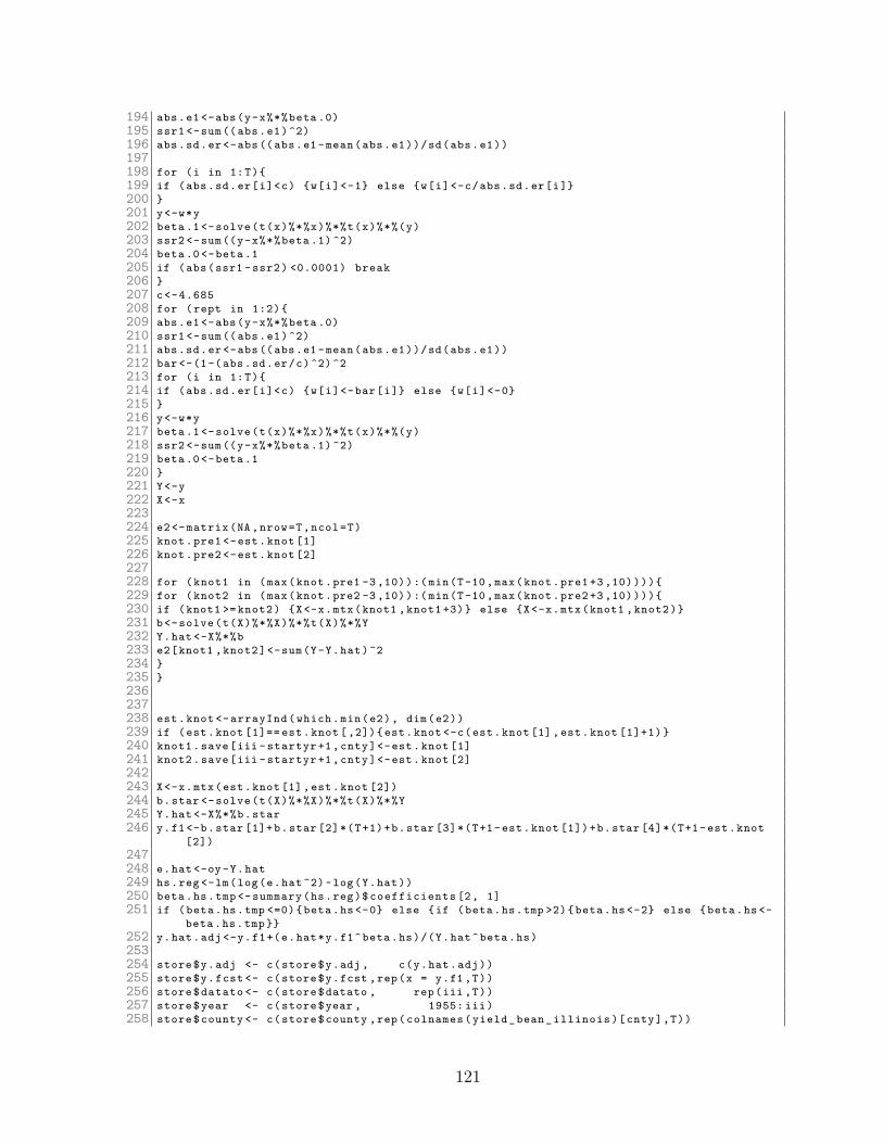
194 abs.e1 <-abs(y-x%*%beta .0)195 ssr1 <-sum (( abs.e1)^2)196 abs.sd.er <-abs (( abs.e1 -mean(abs.e1))/sd(abs.e1))197198 for (i in 1:T){199 if (abs.sd.er[i]<c) {w[i]<-1} else {w[i]<-c/abs.sd.er[i]}200 }201 y<-w*y202 beta .1 <-solve (t(x)%*%x)%*%t(x)%*%(y)203 ssr2 <-sum ((y-x%*%beta .1) ^2)204 beta .0 <-beta .1205 if (abs(ssr1 -ssr2) <0.0001) break206 }207 c<-4.685208 for (rept in 1:2){209 abs.e1 <-abs(y-x%*%beta .0)210 ssr1 <-sum (( abs.e1)^2)211 abs.sd.er <-abs (( abs.e1 -mean(abs.e1))/sd(abs.e1))212 bar <-(1 -( abs.sd.er/c)^2) ^2213 for (i in 1:T){214 if (abs.sd.er[i]<c) {w[i]<-bar[i]} else {w[i]<-0}215 }216 y<-w*y217 beta .1 <-solve (t(x)%*%x)%*%t(x)%*%(y)218 ssr2 <-sum ((y-x%*%beta .1) ^2)219 beta .0 <-beta .1220 }221 Y<-y222 X<-x223224 e2 <-matrix (NA ,nrow=T,ncol=T)225 knot.pre1 <-est.knot [1]226 knot.pre2 <-est.knot [2]227228 for ( knot1 in (max(knot.pre1 -3 ,10)):( min(T -10 , max(knot.pre1 +3 ,10)))){229 for ( knot2 in (max(knot.pre2 -3 ,10)):( min(T -10 , max(knot.pre2 +3 ,10)))){230 if (knot1 >= knot2 ) {X<-x.mtx(knot1 , knot1 +3)} else {X<-x.mtx(knot1 , knot2 )}231 b<-solve (t(X)%*%X)%*%t(X)%*%Y232 Y.hat <-X%*%b233 e2[knot1 , knot2 ]<-sum(Y-Y.hat)^2234 }235 }236237238 est.knot <-arrayInd ( which .min(e2), dim(e2))239 if (est.knot [1]== est.knot [ ,2]){est.knot <-c(est.knot [1] , est.knot [1]+1) }240 knot1 .save[iii - startyr +1, cnty]<-est.knot [1]241 knot2 .save[iii - startyr +1, cnty]<-est.knot [2]242243 X<-x.mtx(est.knot [1] , est.knot [2])244 b.star <-solve (t(X)%*%X)%*%t(X)%*%Y245 Y.hat <-X%*%b.star246 y.f1 <-b.star [1]+b.star [2]*(T+1)+b.star [3]*(T+1- est.knot [1])+b.star [4]*(T+1- est.knot
[2])247248 e.hat <-oy -Y.hat249 hs.reg <-lm(log(e.hat ^2)~log(Y.hat))250 beta.hs.tmp <-summary (hs.reg)$ coefficients [2, 1]251 if (beta.hs.tmp <=0){beta.hs <-0} else {if (beta.hs.tmp >2){beta.hs <-2} else {beta.hs <-
beta.hs.tmp }}252 y.hat.adj <-y.f1 +(e.hat*y.f1^beta.hs)/(Y.hat^beta.hs)253254 store $y.adj <- c( store $y.adj , c(y.hat.adj))255 store $y.fcst <- c( store $y.fcst ,rep(x = y.f1 ,T))256 store $ datato <- c( store $datato , rep(iii ,T))257 store $year <- c( store $year , 1955: iii)258 store $ county <- c( store $county ,rep( colnames ( yield _bean_ illinois )[cnty],T))
121

259 pdf(file = paste (" adjusted _ yields _ illinois _", colnames ( yield _bean_ illinois )[cnty],"_1955 to",iii , ".pdf", sep=""))
260 plot(year [1:( iii -1955+1) ],oy ,ylab=" Yields and Adjusted Yields ",xlab="Year",pch =15 ,ylim=c(min(y.hat.adj ,oy),max(oy ,y.hat.adj)))
261 points (year [1:( iii -1955+1) ],y.hat.adj ,col="red")262 lines (year [1:( iii -1955+1) ],y.hat.adj ,col="red")263 lines (year [1:( iii -1955+1) ],oy ,lty =3)264 lines (year [1:( iii -1955+1) ],Y.hat ,col="grey")265 legend (" topleft ", c(" Adjusted yields "," Yields ","Two - knots Spline "), cex =0.7 ,266 col=c("red"," black ","grey"), pch=c(1 ,15 , NA), lty=c(1 ,3 ,1))267 dev.off ()268 cat("data.av.to=",iii ," county =",cnty.nms[cnty]," ...... ")269 }270271 }272 dev.off ()273 saveRDS ( knot1 .save , file=" saved _ knot1 _bean_ illinois .Rds" ,)274 saveRDS ( knot2 .save , file=" saved _ knot2 _bean_ illinois .Rds" ,)275 saveRDS (store , file=" saved _bean_ illinois .Rds" ,)
adjustdata.R
122

F: R code — Empirical Game
F1: Calculate Premium Rates for Each Estimator
1 load("/home/user/ Dropbox /PhD Essays / Essay II/R code/ empirical game/ yield _ 1955 -2013.Rdata ")
2 tran.grid.den <-function (grid.orig , den.orig , mean.tgt , sd.tgt){3 w<-grid.orig [2] - grid.orig [1]4 mean.orig <-sum(grid.orig*den.orig)*w5 e.x2 <-sum (( grid.orig ^2)*den.orig)*w6 sd.orig <-(e.x2 -mean.orig ^2) ^.57 support .tmp=grid.orig8 lg <-length (grid.orig)9 support <-rep(NA ,lg)
10 for (i in 1: lg){ support [i]<-mean.tgt +( support .tmp[i]-mean.orig)*sd.tgt/sd.orig}11 width2 <-support [2] - support [1]12 width1 <-w13 den <-den.orig* width1 / width214 return ( cbind (support ,den))15 }16 yield _ state _ matrix <- function (data_crop , state ){17 y_ state <- data_crop[data_crop$ state == state , ]18 cnty <- unique (y_ state $ county )19 n_yr <- unique (y_ state $year)20 y_mat <- matrix (0, nrow= length (n_yr), ncol= length (cnty), dimnames =list(sort(n_yr),
cnty))21 for (j in 1: length (cnty)){22 temp <- y_ state [y_ state $ county == colnames (y_mat)[j], ]23 y_mat[, j] <- rev(temp$ yield )24 }25 y_mat <- y_mat[, order ( colnames (y_mat))]26 return (y_mat)27 }28 yield _bean_ illinois <-yield _ state _ matrix (data$bean ," illinois ")29 bean.il. yield _crd_ matrix <-function (dst.n){30 d.crd.i<-matrix (data = (data$bean$ yield [data$bean$ state ==" illinois " & data$bean$ag_
dis == dst.n]) ,byrow =T,31 nrow =2013 -1955+1 ,32 ncol= length ( unique (data$bean$ county [data$bean$ state ==" illinois " & data$bean$ag_dis ==
dst.n])),33 dimnames =list( unique (data$bean$year[data$bean$ state ==" illinois " & data$bean$ag_dis ==
dst.n]) ,34 unique (data$bean$ county [data$bean$ state ==" illinois " & data$bean$ag_dis == dst.n])))35 return (d.crd.i)36 }37 cnty.nms.crdi <-function (dst.n){38 unique (data$bean$ county [data$bean$ state ==" illinois " & data$bean$ag_dis == dst.n])39 }40 ttcnty <-ncol( yield _bean_ illinois )41 cnty.nms <-colnames ( yield _bean_ illinois )42 backyrnum =2043 startyr =2013 - backyrnum44 knot1 .save <-matrix (NA ,nrow= backyrnum +1, ncol=ttcnty ,45 dimnames =list( startyr :2013 ,46 colnames ( yield _bean_ illinois )[1: ttcnty ]))47 knot2 .save <-matrix (NA ,nrow= backyrnum +1, ncol=ttcnty ,48 dimnames =list( startyr :2013 ,49 colnames ( yield _bean_ illinois )[1: ttcnty ]))50 store <-list( datato =NULL ,51 year=NULL ,52 y.adj=NULL ,53 y.fcst=NULL ,54 county =NULL55 )
123

56 for (cnty in 1: ttcnty ) {57 y55to13 <-yield _bean_ illinois [,cnty]58 yield <-y55to1359 year <-rev( unique (data$bean$year))60 y<-y55to13 [1:( startyr -1955+1) ]61 T<-length (y)62 t<-c(1:T)63 x<-matrix (data = 0,nrow = T,ncol =4)64 x<-cbind (1,t,t,t)65 x.mtx <-function (knot1 , knot2 ){66 x<-cbind (1,t,t-knot1 ,t- knot2 )67 x[ ,3][x[ ,3] <0]=068 x[ ,4][x[ ,4] <0]=069 return (x)70 }71 X<-x.mtx (15 ,20)72 Y<-y73 c =1.34574 x<-X75 y<-Y76 beta .0 <-solve (t(x)%*%x)%*%t(x)%*%y77 beta.ols <-beta .078 w<-rep (1,T)79 res <-y-x%*%beta .080 oy <-y81 ox <-x82 for (rept in 1:10^4) {83 abs.e1 <-abs(y-x%*%beta .0)84 ssr1 <-sum (( abs.e1)^2)85 abs.sd.er <-abs (( abs.e1 -mean(abs.e1))/sd(abs.e1))86 for (i in 1:T){87 if (abs.sd.er[i]<c) {w[i]<-1} else {w[i]<-c/abs.sd.er[i]}88 }89 y<-w*y90 beta .1 <-solve (t(x)%*%x)%*%t(x)%*%(y)91 ssr2 <-sum ((y-x%*%beta .1) ^2)92 beta .0 <-beta .193 if (abs(ssr1 -ssr2) <0.0001) break94 c<-4.68595 for (rept in 1:2){96 abs.e1 <-abs(y-x%*%beta .0)97 ssr1 <-sum (( abs.e1)^2)98 abs.sd.er <-abs (( abs.e1 -mean(abs.e1))/sd(abs.e1))99 bar <-(1 -( abs.sd.er/c)^2) ^2
100 for (i in 1:T){101 if (abs.sd.er[i]<c) {w[i]<-bar[i]} else {w[i]<-0}102 }103 y<-w*y104 beta .1 <-solve (t(x)%*%x)%*%t(x)%*%(y)105 ssr2 <-sum ((y-x%*%beta .1) ^2)106 beta .0 <-beta .1107 }108 Y<-y109 X<-x110 e2 <-matrix (NA ,nrow=T,ncol=T)111 for ( knot1 in (10) :(T -15)){112 for ( knot2 in ( knot1 +1) :(T -10)){113 if ( knot1 == knot2 ) {X<-x.mtx(knot1 , knot1 +1)} else {X<-x.mtx(knot1 , knot2 )}114 X<-x.mtx(knot1 , knot2 )115 b<-solve (t(X)%*%X)%*%t(X)%*%Y116 Y.hat <-X%*%b117 e2[knot1 , knot2 ]<-sum(Y-Y.hat)^2118 }119 }120 est.knot <-arrayInd ( which .min(e2), dim(e2))121 knot.pre1 <-est.knot [1]122 knot.pre2 <-est.knot [2]123 for (iii in startyr :2013) {
124

124 y<-y55to13 [1:( iii -1955+1) ]125 T<-length (y)126 t<-c(1:T)127 x<-matrix (data = 0,nrow = T,ncol =4)128 x<-cbind (1,t,t,t)129 x.mtx <-function (knot1 , knot2 ){130 x<-cbind (1,t,t-knot1 ,t- knot2 )131 x[ ,3][x[ ,3] <0]=0132 x[ ,4][x[ ,4] <0]=0133 return (x)134 }135 X<-x.mtx (15 ,20)136 Y<-y137 c =1.345138 x<-X139 y<-Y140 beta .0 <-solve (t(x)%*%x)%*%t(x)%*%y141 beta.ols <-beta .0142 w<-rep (1,T)143 res <-y-x%*%beta .0144 oy <-y145 ox <-x146 for (rept in 1:10^4) {147 abs.e1 <-abs(y-x%*%beta .0)148 ssr1 <-sum (( abs.e1)^2)149 abs.sd.er <-abs (( abs.e1 -mean(abs.e1))/sd(abs.e1))150151 for (i in 1:T){152 if (abs.sd.er[i]<c) {w[i]<-1} else {w[i]<-c/abs.sd.er[i]}153 }154 y<-w*y155 beta .1 <-solve (t(x)%*%x)%*%t(x)%*%(y)156 ssr2 <-sum ((y-x%*%beta .1) ^2)157 beta .0 <-beta .1158 if (abs(ssr1 -ssr2) <0.0001) break159 }160 c<-4.685161 for (rept in 1:2){162 abs.e1 <-abs(y-x%*%beta .0)163 ssr1 <-sum (( abs.e1)^2)164 abs.sd.er <-abs (( abs.e1 -mean(abs.e1))/sd(abs.e1))165 bar <-(1 -( abs.sd.er/c)^2) ^2166 for (i in 1:T){167 if (abs.sd.er[i]<c) {w[i]<-bar[i]} else {w[i]<-0}168 }169 y<-w*y170 beta .1 <-solve (t(x)%*%x)%*%t(x)%*%(y)171 ssr2 <-sum ((y-x%*%beta .1) ^2)172 beta .0 <-beta .1173 }174 Y<-y175 X<-x176 e2 <-matrix (NA ,nrow=T,ncol=T)177 knot.pre1 <-est.knot [1]178 knot.pre2 <-est.knot [2]179 for ( knot1 in (max(knot.pre1 -3 ,10)):( min(T -10 , max(knot.pre1 +3 ,10)))){180 for ( knot2 in (max(knot.pre2 -3 ,10)):( min(T -10 , max(knot.pre2 +3 ,10)))){181 if (knot1 >= knot2 ) {X<-x.mtx(knot1 , knot1 +3)} else {X<-x.mtx(knot1 , knot2 )}182 b<-solve (t(X)%*%X)%*%t(X)%*%Y183 Y.hat <-X%*%b184 e2[knot1 , knot2 ]<-sum(Y-Y.hat)^2185 }186 }187 est.knot <-arrayInd ( which .min(e2), dim(e2))188 if (est.knot [1]== est.knot [ ,2]){est.knot <-c(est.knot [1] , est.knot [1]+1) }189 knot1 .save[iii - startyr +1, cnty]<-est.knot [1]190 knot2 .save[iii - startyr +1, cnty]<-est.knot [2]191
125

192 X<-x.mtx(est.knot [1] , est.knot [2])193 b.star <-solve (t(X)%*%X)%*%t(X)%*%Y194 Y.hat <-X%*%b.star195 y.f1 <-b.star [1]+b.star [2]*(T+1)+b.star [3]*(T+1- est.knot [1])+b.star [4]*(T+1- est.knot
[2])196 e.hat <-oy -Y.hat197 hs.reg <-lm(log(e.hat ^2)~log(Y.hat))198 beta.hs.tmp <-summary (hs.reg)$ coefficients [2, 1]199 if (beta.hs.tmp <=0){beta.hs <-0} else {if (beta.hs.tmp >2){beta.hs <-2} else {beta.hs <-
beta.hs.tmp }}200 y.hat.adj <-y.f1 +(e.hat*y.f1^beta.hs)/(Y.hat^beta.hs)201 store $y.adj <- c( store $y.adj , c(y.hat.adj))202 store $y.fcst <- c( store $y.fcst ,rep(x = y.f1 ,T))203 store $ datato <- c( store $datato , rep(iii ,T))204 store $year <- c( store $year , 1955: iii)205 store $ county <- c( store $county ,rep( colnames ( yield _bean_ illinois )[cnty],T))206 }207 }208 saveRDS ( knot1 .save , file=" saved _ knot1 _bean_ illinois .Rds")209 saveRDS ( knot2 .save , file=" saved _ knot2 _bean_ illinois .Rds")210 saveRDS (store , file=" saved _bean_ illinois .Rds")211 gm.bean. illinois <-readRDS (" saved _bean_ illinois .Rds")212 library (doMC)213 registerDoMC (9)214 getDoParWorkers ()215 crd=c(10 ,20 ,30 ,40 ,50 ,60 ,70 ,80 ,90)216 foreach (n.crd=crd) % dopar % {217 cnty.nms <-cnty.nms.crdi(n.crd)218 fun.y.f1 <-function (cnty , datato ){219 gm.y.f1 <-gm.bean. illinois $y.fcst[gm.bean. illinois $ datato == datato & gm.bean. illinois $
county == cnty]220 return ( unique (gm.y.f1))221 }222 fun.y.adj <-function (cnty , datato ){223 gm.y.adj <-gm.bean. illinois $y.adj[gm.bean. illinois $ datato == datato & gm.bean. illinois $
county == cnty]224 return ( unique (gm.y.adj))225 }226 fun.y.true <-function (cnty , datato ){227 true. yield <-yield _bean_ illinois [ rownames ( yield _bean_ illinois )== datato +1, colnames (
yield _bean_ illinois )== cnty]228 return (true. yield )229 }230 fun.f.cond <-function (h.cv.cond.h,h.cv.cond. lambda ){231 kd <-(h.cv.cond. lambda /(Q -1))^NN*(1-h.cv.cond. lambda )^(1 - NN)232 m.xd <-colMeans (kd)233 ly <-matrix (NA ,nrow=L,ncol= length (grid))234 for (gn in 1: length (grid)){235 ly[,gn]<-1/(h.cv.cond.h)*( dnorm (( grid[gn]-y)/h.cv.cond.h))236 }237 f.xy <-crossprod (ly ,kd)/L238 g.yx <-f.xy/m.xd239 f.cv.cond <-g.yx[, county ]240 f.cv.cond <-f.cv.cond/sum(f.cv.cond* delta )241 return (f.cv.cond)242 }243 fun.f. jones <-function (h. jones .h,h. jones .pool){244 temp1 <-matrix (data=NA ,nrow=n,ncol= length (grid))245 temp2 <-matrix (NA ,nrow= length (samp[, county ]) ,ncol= length (grid))246 for(i in 1: length (grid)){247 temp1 [,i]<-dnorm (( grid[i]-samp[, county ])/h. jones .h)}248 for(i in 1: length (grid)){249 g.hat.x[i]<-1/( length ( sampi )*h. jones .pool)*sum( dnorm (( grid[i]- sampi )/h. jones .pool))250 }251 g.hat.X<-matrix (NA ,nrow= length (samp[, county ]) ,ncol =1)252 for(i in 1: length (samp[, county ])){253 g.hat.X[i]<-1/( length ( sampi )*h. jones .pool)*sum( dnorm (( samp[, county ][i]- sampi )/h. jones
.pool))
126

254 }255 temp2 <-matrix (NA ,nrow= length (samp[, county ]) ,ncol= length (grid))256 for (i in 1: length (grid)){257 temp2 [,i]<-g.hat.x[i]/g.hat.X258 }259 f. jones <-1/(n*h. jones .h)* colSums ( temp1 * temp2 )260 f. jones <-f. jones /sum(f. jones * delta )261 return (f. jones )262 }263 fun.f.psim <-function (h.psim.h,h.psim.pool){264 temp1 <-matrix (data=NA ,nrow=n,ncol= length (grid))265 temp2 <-matrix (NA ,nrow= length (samp[, county ]) ,ncol= length (grid))266 for(i in 1: length (grid)){267 temp1 [,i]<-dnorm (( grid[i]-samp[, county ])/h.psim.h)}268 for(i in 1: length (grid)){269 g.hat.x[i]<-1/( length (pool)*h.psim.pool)*sum( dnorm (( grid[i]-pool)/h.psim.pool))270 }271 g.hat.X<-matrix (NA ,nrow= length (samp[, county ]) ,ncol =1)272 for(i in 1: length (samp[, county ])){273 g.hat.X[i]<-1/( length (pool)*h.psim.pool)*sum( dnorm (( samp[, county ][i]-pool)/h.psim.
pool))274 }275 temp2 <-matrix (NA ,nrow= length (samp[, county ]) ,ncol= length (grid))276 for (i in 1: length (grid)){277 temp2 [,i]<-pmax (.01 , pmin(g.hat.x[i]/g.hat.X ,10))278 }279 f.psim <-1/(n*h.psim.h)* colSums ( temp1 * temp2 )280 f.psim <-f.psim/sum(f.psim* delta )281 return (f.psim)282 }283 fun.f. comb1 <-function (h. comb1 .h,h.cv.cond.h,h.cv.cond. lambda ){284 ly. incomb1 <-matrix (NA ,nrow=L,ncol= length ( sampi ))285 for (gn in 1: length ( sampi )){286 ly. incomb1 [,gn]<-1/(h.cv.cond.h)*( dnorm (( sampi [gn]-y)/h.cv.cond.h))287 }288 kd <-(h.cv.cond. lambda /(Q -1))^NN*(1-h.cv.cond. lambda )^(1 - NN)289 m.xd <-colMeans (kd)290 f.xy. incomb1 <-crossprod (ly.incomb1 ,kd)/L291 g.yx. incomb1 <-f.xy. incomb1 /m.xd292 f.cond.X<-g.yx. incomb1 [, county ]293 h.1 <-h.cv.cond.h294 lambda <-h.cv.cond. lambda295 ly <-matrix (NA ,nrow=L,ncol= length (grid))296 for (gn in 1: length (grid)){297 ly[,gn]<-1/(h.1)*( dnorm (( grid[gn]-y)/h.1))298 }299 f.xy <-crossprod (ly ,kd)/L300 g.yx <-f.xy/m.xd301 f.cv.cond <-g.yx[, county ]302 f.cond.x<-f.cv.cond303 temp2 <-matrix (NA ,nrow= length (samp[, county ]) ,ncol= length (grid))304 for (i in 1: length (grid)){305 temp2 [,i]<-f.cond.x[i]/f.cond.X306 }307 temp1 <-matrix (data=NA ,nrow=n,ncol= length (grid))308 for(i in 1: length (grid)){309 temp1 [,i]<-dnorm (( grid[i]-samp[, county ])/h. comb1 .h)}310 f.cv. comb1 <-1/(n*h. comb1 .h)* colSums ( temp1 * temp2 )311 f.cv. comb1 <-f.cv. comb1 /sum(f.cv. comb1 * delta )312 return (f.cv. comb1 )313 }314 fun.f. comb2 <-function (lambda ,h,h.pool){315 {316 kd <-( lambda /(Q -1))^NN*(1- lambda )^(1 - NN)317 kd.part <-kd[, county ]318 for (gn in 1: lg){319 kd.part.m[gn ,] <-kd.part}320 for (gn in 1: lg){
127

321 k.part.m[gn ,] <-dnorm (( grid[gn]-pool)/h)}322 for (i in 1:L)323 {324 g.Y[i ,] <-1/(h.pool*L)*sum( dnorm (( pool[i]-pool)/h.pool))325 }326 for (gn in 1: lg){327 g.grid.i<-1/(h.pool*L)*sum( dnorm (( grid[gn]-pool)/h.pool))328 g.part.m[gn ,] <-g.grid.i/g.Y329 }330 f. comb2 <-1/(L*h)* rowSums (kd.part.m*k.part.m*g.part.m)331 f. comb2 <-f. comb2 /sum(f. comb2 * delta )332 }333 return (f. comb2 )334 }335 function .cv.kde <-function (h.kde){336 {337 for (i in 1: length ( sampi )){338 f.kde.cv[i]<- 1/((n -1)*h.kde)*(sum( dnorm (( sampi - sampi [i])/h.kde))-dnorm (0)) }339 }340 -sum(log(f.kde.cv))341 }342 function .cv.kde.all <-function (h.kde.all){343 {344 for (i in 1: length (pool)){345 f.kde.all.cv[i]<- 1/((L -1)*h.kde.all)*(sum( dnorm (( pool -pool[i])/h.kde.all))-dnorm (0))346 }347 }348 -sum(log(f.kde.all.cv))349 }350 function .cv.cond <-function (h){351 {352 h.1 <-abs(h[1])353 lambda <-pnorm (h[2])*up354 kd <-( lambda /(Q -1))^NN*(1- lambda )^(1 - NN)355 m.xd <-colMeans (kd)356 for (gn in 1: length (pool)){357 ly[,gn]<-1/(h.1)*( dnorm (( pool[gn]-y)/h.1))358 }359 cprod <-crossprod (ly ,kd)360 g.cv.all.nu <-cprod -(1 - lambda )*1/h.1* dnorm (0)361 g.cv.all.de <-(n+lambda -1)/(n*Q -1)362 g.cv.all <-1/(n*Q -1)*g.cv.all.nu/g.cv.all.de363 cv.prob <-g.cv.all*(1-NN)364 p.all.cnty. happen <-rowSums (cv.prob)365 p.own.cnty. happen <-cv.prob [(( county -1)*n+1) :( county *n),county ]366 }367 -sum(log(p.all.cnty. happen ))368 }369 function .cv.r. jones <-function (h){370 {371 h.k<-h372 h. jones .pool <-h373 for(i in 1: length ( sampi )){374 temp1 [,i]<-dnorm (( sampi [i]- sampi )/h.k)}375 for(i in 1: length ( sampi )){376 g.hat.x[i]<-1/(( length ( sampi ))*h. jones .pool)*(sum( dnorm (( sampi [i]- sampi )/h. jones .pool
)))377 }378 g.hat.X<-g.hat.x379 temp2 <-matrix (NA ,nrow= length (samp[, county ]) ,ncol= length ( sampi ))380 for (i in 1: length ( sampi )){381 temp2 [,i]<-g.hat.x[i]/g.hat.X382 }383 f.new <-1/((n -1)*h.k)*( colSums ( temp1 * temp2 )-dnorm (0))384 }385 -sum(log(f.new))386 }387 function .cv.psim <-function (bw){
128

388 {389 h<-bw [1]390 h.psim.pool <-bw [2]391 for(i in 1: length ( sampi )){392 g.hat.x[i]<-1/(( length (pool) -1)*h.psim.pool)*sum( dnorm (( sampi [i]-pool)/h.psim.pool))393 }394 g.hat.X<-g.hat.x395 for (i in 1: length ( sampi )){396 temp2 [,i]<-g.hat.x[i ,]/g.hat.X397 }398 for(i in 1: length ( sampi )){399 temp1 [,i] <- dnorm (( sampi [i]- sampi )/h)}400 f.new <- 1/((n -1)*h)*( colSums ( temp1 * temp2 )-dnorm (0))401 }402 -sum(log(f.new))403 }404 function .cv. comb1 .hh <-function (h){405 {406 hk <-h[1]407 h.cv.cond.h<-h[2]408 h.cv.cond. lambda <-h[3]409410 for (gn in 1: length ( sampi )){411 ly. incomb1 [,gn]<-1/(h.cv.cond.h)*( dnorm (( sampi [gn]-y)/h.cv.cond.h))}412413 kd <-(h.cv.cond. lambda /(Q -1))^NN*(1-h.cv.cond. lambda )^(1 - NN)414 m.xd <-colMeans (kd)415 f.xy. incomb1 <-crossprod (ly.incomb1 ,kd)/L416 g.yx. incomb1 <-f.xy. incomb1 /m.xd417 f.cond.X<-g.yx. incomb1 [, county ]418 for (i in 1:n){419 temp2 [,i]<-f.cond.X[i]/f.cond.X420 }421422 for(i in 1:n){ temp1 [,i]<-dnorm (( sampi [i]- sampi )/hk)}423424 f.new <-1/((n -1)*hk)*( colSums ( temp1 * temp2 )-dnorm (0))425 }426 return (-sum(log(f.new)))427 }428 function .cv. comb2 .f.lmd <-function (h){429 {430 h.k<-h[1]431 h.pool <-h[2]432 lambda <-h[3]433 kd <-( lambda /(Q -1))^NN*(1- lambda )^(1 - NN)434 kd.part <-kd[, county ]435 for (gn in 1: length (pool)){436 kd.part.m[gn ,] <-kd.part437 k.part.m[gn ,] <-as. matrix ( dnorm (( pool[gn]-pool)/h.k))438 }439440 for (i in 1:L)441 {g.Y[i ,] <-1/(h.pool*L)*sum( dnorm (( pool[i]-pool)/h.pool))}442 for (gn in 1: length (pool)){443 g.grid.i<-1/(h.pool*L)*sum( dnorm (( pool[gn]-pool)/h.pool))444 g.part.m[gn ,] <-g.grid.i/g.Y445 }446 AAA <-(kd.part.m*k.part.m)447 BBB <-AAA*g.part.m448 f. comb2 .all <-1/((L -1)*h.k)*( rowSums (BBB) -(1- lambda )* dnorm (0))449450 f. comb2 . ocnty <-f. comb2 .all [(( county -1)*n+1) :( county *n)]451 }452 -sum(log(f. comb2 . ocnty ))453 }454455 cl =0.9
129

456 y.act <-matrix (0 ,20 , length (cnty.nms))457 y.gaur <-y.act458 loss <-y.act459 rate.e<-y.act460 rate.kde <-y.act461 rate.kde.all <-y.act462 rate. jones <-y.act463 rate.psim <-y.act464 rate.cond <-y.act465 rate. comb1 <-y.act466 rate. comb2 <-y.act467 gm.st.yr =2012 -20+1468 for ( datato in gm.st.yr :2012) {469 dav <-datato -gm.st.yr +1470 for ( county in 1: length (cnty.nms)){471 year <-1955: datato472 cnty=cnty.nms[ county ]473 fcst. yield <-fun.y.f1(cnty , datato )474 true. yield <-fun.y.true(cnty , datato )475 y.adj.pre <-fun.y.adj(cnty , datato )476 y.g<-fcst. yield *cl477 y.gaur[dav , county ]<-y.g478 loss[dav , county ]<-max(y.g-true.yield ,0)479 rate.e[dav , county ]<-sum(pmax(y.g-y.adj.pre ,0))/ length (y.adj.pre)480 samp.orgn <-matrix (NA ,nrow= length (y.adj.pre),ncol= length (cnty.nms),dimnames =list(year ,
cnty.nms))481 for (i in 1: length (cnty.nms))482 {483 samp.orgn[,i]<-fun.y.adj(cnty.nms[i], datato )484 }485 Q<-ncol(samp.orgn)486 n<-n.av <-nrow(samp.orgn)487 mean.all <-colMeans (samp.orgn)488 sd.all <-diag(var(samp.orgn))^.5489 samp.std <-samp.orgn490 for (j in 1:Q){samp.std[,j]<-(samp.orgn[,j]-mean.all[j])/sd.all[j]}491492 mi <-mean.all[ county ]493 si <-sd.all[ county ]494 samp.t<-samp.std*si+mi495 pool <-c(samp.std)496 samp <-samp.std497 sampi <-as. matrix (samp.std[, county ])498 L<-n*Q499 lowlim <-0.1500 uplim <-1000501 up <-((Q -1)/Q)502 lambda .set.to <-up503 nbs <-n504 bsss <-n -1505 grid.std <-seq ( -800 ,800)/100506 grid <-grid.std507 lg <-length (grid)508 delta <-grid [2] - grid [1]509 f.kde.cv <-sampi510 kde <- optimize ( function .cv.kde ,c(lowlim , uplim ))511 h.cv.kde <-kde$ minimum512 f.kde <-grid513 for (i in 1: length (grid)){514 f.kde[i]<-1/(n*h.cv.kde)*sum( dnorm (( sampi -grid[i])/h.cv.kde))515 }516 f.cv.kde <-f.kde/sum(f.kde* delta )517 f.kde.all.cv <-pool518 opt.kde.all <- optimize ( function .cv.kde.all ,c(lowlim , uplim ))519 h.cv.kde.all <-opt.kde.all$ minimum520 f.kde.all <-f.kde521 for (i in 1: length (grid)){522 f.kde.all[i]<-1/(n*Q*h.cv.kde.all)*sum( dnorm (( pool -grid[i])/h.cv.kde.all))
130
523 }524 f.cv.kde.all <-f.kde.all/sum(f.kde.all* delta )525 y<-c(pool)526 x<-matrix (NA ,nrow=n,ncol=Q)527 for (i in 1:Q){528 x[,i]<-rep ((i -1) ,n)529 }530 x<-factor (x)531 NN <-matrix (1,L,Q)532 for (j in 1:Q){533 NN [(n.av*(j -1) +1) :((n.av*(j -1) +1)+n.av -1) ,j]<-rep (0,n.av)534 }535 ly <-matrix (NA ,L,L)536 ly <-matrix (NA ,nrow=L,ncol=L)537 start .cond <-c(h.cv.kde ,up/2)538 opt.cv.cond <-optim ( start .cond , function .cv.cond)539540 h.cv.cond.h <-abs(opt.cv.cond$par [1])541 h.cv.cond. lambda <-pnorm (opt.cv.cond$par [2])*up542 f.cv.cond <-fun.f.cond(h.cv.cond.h,h.cv.cond. lambda )543544 # Jones start ---545 g.hat.x<-matrix (NA ,nrow=n,ncol =1)546 temp1 <-matrix (data=NA ,nrow=n,ncol=n)547 opt. jones <- optimize (f= function .cv.r.jones , interval = c(lowlim , uplim ))548 h. jones .r.h <-opt. jones $ minimum549 h. jones .r.pool <-opt. jones $ minimum550 f.cv. jones <-fun.f. jones (h. jones .r.h,h. jones .r.pool)551 # possible similar start ------552 temp2 <-matrix (NA ,nrow= length ( sampi ),ncol=n)553 temp1 <-matrix (data=NA ,nrow=n,ncol=n)554 opt.psim <- optim (par = c(2*h.cv.kde ,h.cv.kde),fn = function .cv.psim , method ="L-BFGS -B"
,555 lower =c(h.cv.kde*1.5 ,h.cv.kde*.8) ,556 upper =c(h.cv.kde*2.5 ,100)557 )558 h.psim.h <-opt.psim$par [1]559 h.psim.pool <-opt.psim$par [2]560561 f.cv.psim <-fun.f.psim(h.psim.h,h.psim.pool)562 #comb1 ----563 ly. incomb1 <-matrix (NA ,nrow=L,ncol= length ( sampi ))564 temp2 <-matrix (NA ,nrow= length ( sampi ),ncol=n)565 temp1 <-matrix (data=NA ,nrow=n,ncol=n)566 s1 =2*h.cv.kde; s2=h.cv.kde; s3=up*.8567 l1 =1.5*h.cv.kde; l2 =.8*h.cv.kde; l3 =0568 u1 =2.5*h.cv.kde; u2 =100; u3=up569 opt.cb1.hh <-optim (par =c(s1 ,s2 ,s3),fn = function .cv. comb1 .hh ,570 method = "L-BFGS -B",571 lower = c(l1 ,l2 ,l3),572 upper = c(u1 ,u2 ,u3))573 h.cv.cb1.hh.hk <-opt.cb1.hh$par [1]574 h.cv.cb1.hh.ch <-opt.cb1.hh$par [2]575 h.cv.cb1.hh.clmd <-opt.cb1.hh$par [3]576 f.cv. comb1 <-fun.f. comb1 (h.cv.cb1.hh.hk ,h.cv.cb1.hh.ch ,h.cv.cb1.hh.clmd)577 # comb2 .cv start -----578 f. comb2 <-matrix (NA ,nrow=lg ,ncol =1)579 g.Y<-matrix (NA ,nrow=L,ncol =1)580 kd.part.m<-matrix (NA ,nrow=L,ncol=L)581 k.part.m<-matrix (NA ,nrow=L,ncol=L)582 g.part.m<-matrix (NA ,nrow=L,ncol=L)583 s1=h.cv.cond.h; s2 =10; s3=h.cv.cond. lambda584 l1=h.cv.cond.h; l2 =0.2; l3 =0585 u1 =1.5*h.cv.cond.h; u2 =20; u3=up586 opt. comb2 .cv.f.lmd <-optim (par =c(s1 ,s2 ,s3),fn = function .cv. comb2 .f.lmd ,587 method = "L-BFGS -B",588 lower = c(l1 ,l2 ,l3),589 upper = c(u1 ,u2 ,u3))
131

590 h. comb2 .cv.f.lmd.h.k <-opt. comb2 .cv.f.lmd$par [1]591 h. comb2 .cv.f.lmd.h.pool <-opt. comb2 .cv.f.lmd$par [2]592 h. comb2 .cv.f.lmd. lambda <-opt. comb2 .cv.f.lmd$par [3]593 f. comb2 .cv <-matrix (NA ,nrow=lg ,ncol =1)594 g.Y<-matrix (NA ,nrow=L,ncol =1)595 kd.part.m<-matrix (NA ,nrow=lg ,ncol=L)596 k.part.m<-matrix (NA ,nrow=lg ,ncol=L)597 g.part.m<-matrix (NA ,nrow=lg ,ncol=L)598 f.cv. comb2 <-fun.f. comb2 (h. comb2 .cv.f.lmd.lambda ,h. comb2 .cv.f.lmd.h.k,h. comb2 .cv.f.lmd
.h.pool)599600 f.cv.kde <-tran.grid.den(grid.orig = grid , den.orig = f.cv.kde , mean.tgt = mi ,sd
.tgt = si)601 f.cv.kde.all <-tran.grid.den(grid.orig = grid ,den.orig = f.cv.kde.all , mean.tgt =
mi ,sd.tgt = si)602 f.cv.cond <-tran.grid.den(grid.orig = grid , den.orig = f.cv.cond , mean.tgt = mi ,
sd.tgt = si)603 f.cv. jones <-tran.grid.den(grid.orig = grid , den.orig = f.cv.jones , mean.tgt = mi ,
sd.tgt = si)604 f.cv.psim <-tran.grid.den(grid.orig = grid , den.orig = f.cv.psim , mean.tgt = mi ,
sd.tgt = si)605 f.cv. comb1 <-tran.grid.den(grid.orig = grid , den.orig = f.cv.comb1 , mean.tgt = mi ,
sd.tgt = si)606 f.cv. comb2 <-tran.grid.den(grid.orig = grid , den.orig = f.cv.comb2 , mean.tgt = mi ,
sd.tgt = si)607608 ## calculate primum rate of each estimated density609 w.kde <-f.cv.kde [2 ,1] -f.cv.kde [1 ,1]610 rate.kde[dav , county ]<-sum (( pmax(y.g-f.cv.kde [ ,1] ,0))*f.cv.kde [ ,2]*w.kde)611612 w.kde.all <-f.cv.kde.all [2 ,1] -f.cv.kde.all [1 ,1]613 rate.kde.all[dav , county ]<-sum (( pmax(y.g-f.cv.kde.all [ ,1] ,0))*f.cv.kde.all [ ,2]*w.kde.
all)614615 w. jones <-f.cv. jones [2 ,1] -f.cv. jones [1 ,1]616 rate. jones [dav , county ]<-sum (( pmax(y.g-f.cv. jones [ ,1] ,0))*f.cv. jones [ ,2]*w. jones )617618 w.psim <-f.cv.psim [2 ,1] -f.cv.psim [1 ,1]619 rate.psim[dav , county ]<-sum (( pmax(y.g-f.cv.psim [ ,1] ,0))*f.cv.psim [ ,2]*w.psim)620621 w.cond <-f.cv.cond [2 ,1] -f.cv.cond [1 ,1]622 rate.cond[dav , county ]<-sum (( pmax(y.g-f.cv.cond [ ,1] ,0))*f.cv.cond [ ,2]*w.cond)623624 w. comb1 <-f.cv. comb1 [2 ,1] -f.cv. comb1 [1 ,1]625 rate. comb1 [dav , county ]<-sum (( pmax(y.g-f.cv. comb1 [ ,1] ,0))*f.cv. comb1 [ ,2]*w. comb1 )626627 w. comb2 <-f.cv. comb2 [2 ,1] -f.cv. comb2 [1 ,1]628 rate. comb2 [dav , county ]<-sum (( pmax(y.g-f.cv. comb2 [ ,1] ,0))*f.cv. comb2 [ ,2]*w. comb2 )629630 }631 }632 rate.crdi <-list(633 emp=rate.e,634 kde=rate.kde ,635 kde.all=rate.kde.all ,636 jones =rate.jones ,637 psim=rate.psim ,638 cond=rate.cond ,639 loss=loss ,640 comb1 =rate.comb1 ,641 comb2 =rate. comb2642 )643 saveRDS ( object = rate.crdi ,file = paste ("rate.all.crd",n.crd ,".rds",sep = "") )644 }
RcodeEmpiricalGameCalculatePremiumRatesforEachEstimator.r
132
F2: Comparing Rates from Different Estimators
1 library (" xtable ")2 load("/home/user/ Dropbox /PhD Essays / Essay II/R code/ empirical game/ yield _ 1955 -2013.
Rdata ")3 cnty.nms.crdi <-function (dst.n){4 unique (data$corn$ county [data$corn$ state ==" illinois " & data$corn$ag_dis == dst.n])5 }6 ctnm <-c(cnty.nms.crdi (10) ,7 cnty.nms.crdi (20) ,8 cnty.nms.crdi (30) ,9 cnty.nms.crdi (40) ,
10 cnty.nms.crdi (50) ,11 cnty.nms.crdi (60) ,12 cnty.nms.crdi (70) ,13 cnty.nms.crdi (80) ,14 cnty.nms.crdi (90))15 wt <-readRDS ("IL.corn. weight _82 counties .rds")16 wtx <-rep(NA , length (wt$ weight ))17 for (i in 1: length (wt$ weight )){18 wtx[i]<-wt$ weight [ weight $cnty.nm == ctnm[i]]19 }20 crd10 <-readRDS ("rate.all. crd10 .rds")21 crd20 <-readRDS ("rate.all. crd20 .rds")22 crd30 <-readRDS ("rate.all. crd30 .rds")23 crd40 <-readRDS ("rate.all. crd40 .rds")24 crd50 <-readRDS ("rate.all. crd50 .rds")25 crd60 <-readRDS ("rate.all. crd60 .rds")26 crd70 <-readRDS ("rate.all. crd70 .rds")27 crd80 <-readRDS ("rate.all. crd80 .rds")28 crd90 <-readRDS ("rate.all. crd90 .rds")29 emp <-cbind ( crd10 $emp ,30 crd20 $emp ,31 crd30 $emp ,32 crd40 $emp ,33 crd50 $emp ,34 crd60 $emp ,35 crd70 $emp ,36 crd80 $emp ,37 crd90 $emp)38 kde <-cbind ( crd10 $kde ,39 crd20 $kde ,40 crd30 $kde ,41 crd40 $kde ,42 crd50 $kde ,43 crd60 $kde ,44 crd70 $kde ,45 crd80 $kde ,46 crd90 $kde)47 kde.all <-cbind ( crd10 $kde.all ,48 crd20 $kde.all ,49 crd30 $kde.all ,50 crd40 $kde.all ,51 crd50 $kde.all ,52 crd60 $kde.all ,53 crd70 $kde.all ,54 crd80 $kde.all ,55 crd90 $kde.all)56 jones <-cbind ( crd10 $jones ,57 crd20 $jones ,58 crd30 $jones ,59 crd40 $jones ,60 crd50 $jones ,61 crd60 $jones ,62 crd70 $jones ,63 crd80 $jones ,
133

64 crd90 $ jones )65 psim <-cbind ( crd10 $psim ,66 crd20 $psim ,67 crd30 $psim ,68 crd40 $psim ,69 crd50 $psim ,70 crd60 $psim ,71 crd70 $psim ,72 crd80 $psim ,73 crd90 $psim)74 cond <-cbind ( crd10 $cond ,75 crd20 $cond ,76 crd30 $cond ,77 crd40 $cond ,78 crd50 $cond ,79 crd60 $cond ,80 crd70 $cond ,81 crd80 $cond ,82 crd90 $cond)83 comb1 <-cbind ( crd10 $comb1 ,84 crd20 $comb1 ,85 crd30 $comb1 ,86 crd40 $comb1 ,87 crd50 $comb1 ,88 crd60 $comb1 ,89 crd70 $comb1 ,90 crd80 $comb1 ,91 crd90 $ comb1 )92 comb2 <-cbind ( crd10 $comb2 ,93 crd20 $comb2 ,94 crd30 $comb2 ,95 crd40 $comb2 ,96 crd50 $comb2 ,97 crd60 $comb2 ,98 crd70 $comb2 ,99 crd80 $comb2 ,
100 crd90 $ comb2 )101102 loss <-cbind ( crd10 $loss ,103 crd20 $loss ,104 crd30 $loss ,105 crd40 $loss ,106 crd50 $loss ,107 crd60 $loss ,108 crd70 $loss ,109 crd80 $loss ,110 crd90 $loss)111112 m=20; nc=ncol(emp)113 results .f<-function (r1 ,r2) {114 ww <-matrix (0,m,nc)115 ww[r2 <r1]<-1116 percent <-sum(ww)/(m*nc)117 loss <-sweep (x = loss , MARGIN = 2, STATS = wtx ,FUN = ’*’)118 r1 <-sweep (x = r1 , MARGIN = 2, STATS = wtx ,FUN = ’*’)119 prog.lr <-sum(loss)/sum(r1)120 ins.lr <-sum(ww*loss)/sum(ww*r1)121 ww .1 <-1-ww122 gov.lr <-sum(ww .1*loss)/sum(ww .1*r1)123 ins.lr.test <-rep (0 ,1000)124 for (i in 1:1000) {125 ww.test <-matrix ( runif (m*nc),m,nc)126 ww.temp <-matrix (0,m,nc)127 ww.temp[ww.test < percent ]<-1128 ins.lr.test[i]<-sum(ww.temp*loss)/sum(ww.temp*r1)129 }130 pval <-rep (0 ,1000)131 pval[ins.lr.test <ins.lr]<-1
134

132 pvalue <-mean(pval)133 final <-c(prog.lr ,ins.lr ,gov.lr ,percent , pvalue )134 return ( final )}135 all. rates <-list( Empirical =emp ,136 KDE=kde ,137 KDE.all=kde.all ,138 Jones =jones ,139 KerPS =psim ,140 Cond=cond ,141 Comb1 =comb1 ,142 Comb2 = comb2 )143 for (j in 1: length (all. rates )){144 out <-matrix (NA ,nrow = length (all. rates ),ncol =5, dimnames = list(c( names (all. rates )),c(
"prog.lr","ins.lr","gov.lr"," percent "," pvalue ")))145 for (i in 1: length (all. rates )){146 out[i ,] <-results .f(all. rates [[i]], all. rates [[j]])147 }148 cpt= paste (" Pseudo Insurance Company Rate from",names (all. rates )[j])149 print ( xtable (out , caption = cpt))150 }151 results .f(psim ,kde)
RcodeEmpiricalGameCompareRatesfromDifferentEstimators.r
135

G: R code — Sensitivity Analysis
G1: Sensitivity Analysis: Comparing Rates fromDifferent Estimators
1 library (" xtable ")2 load("/home/user/ Dropbox /PhD Essays / Essay II/R code/ empirical game/ yield _ 1955 -2013.
Rdata ")3 cnty.nms.crdi <-function (dst.n){4 unique (data$bean$ county [data$bean$ state ==" illinois " & data$bean$ag_dis == dst.n])5 }6 ctnm <-c(cnty.nms.crdi (10) ,7 cnty.nms.crdi (20) ,8 cnty.nms.crdi (30) ,9 cnty.nms.crdi (40) ,
10 cnty.nms.crdi (50) ,11 cnty.nms.crdi (60) ,12 cnty.nms.crdi (70) ,13 cnty.nms.crdi (80) ,14 cnty.nms.crdi (90))15 wt <-readRDS ("IL.bean. weight _82 counties .rds")16 wtx <-rep(NA , length (wt$ weight ))17 for (i in 1: length (wt$ weight )){18 wtx[i]<-wt$ weight [ weight $cnty.nm == ctnm[i]]19 }20 wtx <-rep (1, length (ctnm))/ length (ctnm)21 crd10 <-readRDS ("rate.all.crd .10 rct.yr10.rds")22 crd20 <-readRDS ("rate.all.crd .20 rct.yr10.rds")23 crd30 <-readRDS ("rate.all.crd .30 rct.yr10.rds")24 crd40 <-readRDS ("rate.all.crd .40 rct.yr10.rds")25 crd50 <-readRDS ("rate.all.crd .50 rct.yr10.rds")26 crd60 <-readRDS ("rate.all.crd .60 rct.yr10.rds")27 crd70 <-readRDS ("rate.all.crd .70 rct.yr10.rds")28 crd80 <-readRDS ("rate.all.crd .80 rct.yr10.rds")29 crd90 <-readRDS ("rate.all.crd .90 rct.yr10.rds")30 emp <-cbind ( crd10 $emp ,31 crd20 $emp ,32 crd30 $emp ,33 crd40 $emp ,34 crd50 $emp ,35 crd60 $emp ,36 crd70 $emp ,37 crd80 $emp ,38 crd90 $emp)3940 kde <-cbind ( crd10 $kde ,41 crd20 $kde ,42 crd30 $kde ,43 crd40 $kde ,44 crd50 $kde ,45 crd60 $kde ,46 crd70 $kde ,47 crd80 $kde ,48 crd90 $kde)4950 kde.all <-cbind ( crd10 $kde.all ,51 crd20 $kde.all ,52 crd30 $kde.all ,53 crd40 $kde.all ,54 crd50 $kde.all ,55 crd60 $kde.all ,56 crd70 $kde.all ,
136
57 crd80 $kde.all ,58 crd90 $kde.all)5960 jones <-cbind ( crd10 $jones ,61 crd20 $jones ,62 crd30 $jones ,63 crd40 $jones ,64 crd50 $jones ,65 crd60 $jones ,66 crd70 $jones ,67 crd80 $jones ,68 crd90 $ jones )6970 psim <-cbind ( crd10 $psim ,71 crd20 $psim ,72 crd30 $psim ,73 crd40 $psim ,74 crd50 $psim ,75 crd60 $psim ,76 crd70 $psim ,77 crd80 $psim ,78 crd90 $psim)7980 cond <-cbind ( crd10 $cond ,81 crd20 $cond ,82 crd30 $cond ,83 crd40 $cond ,84 crd50 $cond ,85 crd60 $cond ,86 crd70 $cond ,87 crd80 $cond ,88 crd90 $cond)8990 comb1 <-cbind ( crd10 $comb1 ,91 crd20 $comb1 ,92 crd30 $comb1 ,93 crd40 $comb1 ,94 crd50 $comb1 ,95 crd60 $comb1 ,96 crd70 $comb1 ,97 crd80 $comb1 ,98 crd90 $ comb1 )99
100 comb2 <-cbind ( crd10 $comb2 ,101 crd20 $comb2 ,102 crd30 $comb2 ,103 crd40 $comb2 ,104 crd50 $comb2 ,105 crd60 $comb2 ,106 crd70 $comb2 ,107 crd80 $comb2 ,108 crd90 $ comb2 )109110 loss <-cbind ( crd10 $loss ,111 crd20 $loss ,112 crd30 $loss ,113 crd40 $loss ,114 crd50 $loss ,115 crd60 $loss ,116 crd70 $loss ,117 crd80 $loss ,118 crd90 $loss)119 m=20; nc=ncol(emp)120 results .f<-function (r1 ,r2) {121122 ww <-matrix (0,m,nc)123 ww[r2 <r1]<-1124 percent <-sum(ww)/(m*nc)
137

125 loss <-sweep (x = loss , MARGIN = 2, STATS = wtx ,FUN = ’*’)126 r1 <-sweep (x = r1 , MARGIN = 2, STATS = wtx ,FUN = ’*’)127 prog.lr <-sum(loss)/sum(r1)128 ins.lr <-sum(ww*loss)/sum(ww*r1)129 ww .1 <-1-ww130 gov.lr <-sum(ww .1*loss)/sum(ww .1*r1)131 ins.lr.test <-rep (0 ,1000)132 for (i in 1:1000) {133 ww.test <-matrix ( runif (m*nc),m,nc)134 ww.temp <-matrix (0,m,nc)135 ww.temp[ww.test < percent ]<-1136 ins.lr.test[i]<-sum(ww.temp*loss)/sum(ww.temp*r1)137 }138 pval <-rep (0 ,1000)139 pval[ins.lr.test <ins.lr]<-1140 pvalue <-mean(pval)141 final <-c(prog.lr ,ins.lr ,gov.lr ,percent , pvalue )142 return ( final )}143144 all. rates <-list( Empirical =emp ,145 KDE=kde ,146 KDE.all=kde.all ,147 Jones =jones ,148 KerPS =psim ,149 Cond=cond ,150 Comb1 =comb1 ,151 Comb2 = comb2 )152 for (j in 1: length (all. rates )){153 out <-matrix (NA ,nrow = length (all. rates ),ncol =5, dimnames = list(c( names (all. rates )),c(
"prog.lr","ins.lr","gov.lr"," percent "," pvalue ")))154 for (i in 1: length (all. rates )){155 out[i ,] <-results .f(all. rates [[i]], all. rates [[j]])156 }157 cpt= paste (" Pseudo Insurance Company Rate from",names (all. rates )[j])158 print ( xtable (out , caption = cpt))159 }
RcodeSensitivityAnalysisComparingRatesfromDifferentEstimators.r
G2: Sensitivity Analysis Calculate Rates for EachEstimator
1 load("/home/user/ Dropbox /PhD Essays / Essay II/R code/ empirical game/ yield _ 1955 -2013.Rdata ")
2 tran.grid.den <-function (grid.orig , den.orig , mean.tgt , sd.tgt){3 w<-grid.orig [2] - grid.orig [1]4 mean.orig <-sum(grid.orig*den.orig)*w #mean of grid.f5 e.x2 <-sum (( grid.orig ^2)*den.orig)*w # square mean of grid.f6 sd.orig <-(e.x2 -mean.orig ^2) ^.57 support .tmp=grid.orig8 lg <-length (grid.orig)9 support <-rep(NA ,lg)
10 for (i in 1: lg){ support [i]<-mean.tgt +( support .tmp[i]-mean.orig)*sd.tgt/sd.orig}11 width2 <-support [2] - support [1]12 width1 <-w13 den <-den.orig* width1 / width214 return ( cbind (support ,den))15 }16 yield _ state _ matrix <- function (data_crop , state ){17 y_ state <- data_crop[data_crop$ state == state , ]18 cnty <- unique (y_ state $ county )19 n_yr <- unique (y_ state $year)
138
20 y_mat <- matrix (0, nrow= length (n_yr), ncol= length (cnty), dimnames =list(sort(n_yr),cnty))
21 for (j in 1: length (cnty)){22 temp <- y_ state [y_ state $ county == colnames (y_mat)[j], ]23 y_mat[, j] <- rev(temp$ yield )24 }25 y_mat <- y_mat[, order ( colnames (y_mat))]26 return (y_mat)27 }28 yield _bean_ illinois <-yield _ state _ matrix (data$bean ," illinois ")29 bean.il. yield _crd_ matrix <-function (dst.n){30 d.crd.i<-matrix (data = (data$bean$ yield [data$bean$ state ==" illinois " & data$bean$ag_
dis == dst.n]) ,byrow =T,31 nrow =2013 -1955+1 ,32 ncol= length ( unique (data$bean$ county [data$bean$ state ==" illinois " & data$bean$ag_dis ==
dst.n])),33 dimnames =list( unique (data$bean$year[data$bean$ state ==" illinois " & data$bean$ag_dis ==
dst.n]) ,34 unique (data$bean$ county [data$bean$ state ==" illinois " & data$bean$ag_dis == dst.n])))35 return (d.crd.i)36 }37 cnty.nms.crdi <-function (dst.n){38 unique (data$bean$ county [data$bean$ state ==" illinois " & data$bean$ag_dis == dst.n])39 }40 # adjust the original yield data ======41 #detrend , adjust heteroscedasticity42 ttcnty <-ncol( yield _bean_ illinois )43 cnty.nms <-colnames ( yield _bean_ illinois )44 backyrnum =20 #run the game for 20 times45 n.av.yrs =30 # assume only have most recent (n.av.yrs) years of data46 startyr =2013 - backyrnum47 knot1 .save <-matrix (NA ,nrow= backyrnum +1, ncol=ttcnty ,48 dimnames =list( startyr :2013 ,49 colnames ( yield _bean_ illinois )[1: ttcnty ]))50 knot2 .save <-matrix (NA ,nrow= backyrnum +1, ncol=ttcnty ,51 dimnames =list( startyr :2013 ,52 colnames ( yield _bean_ illinois )[1: ttcnty ]))5354 store <-list( datato =NULL ,55 year=NULL ,56 y.adj=NULL ,57 y.fcst=NULL ,58 county =NULL59 )6061 for (cnty in 1: ttcnty ) {6263 y55to13 <-yield _bean_ illinois [,cnty]64 yield <-y55to1365 year <-rev( unique (data$bean$year))66 y<-y55to13 [( startyr -1955+1 -n.av.yrs +1) :( startyr -1955+1) ]67 T<-length (y)68 t<-c(1:T)69 x<-matrix (data = 0,nrow = T,ncol =4)70 x<-cbind (1,t,t,t)71 x.mtx <-function (knot1 , knot2 ){72 x<-cbind (1,t,t-knot1 ,t- knot2 )73 x[ ,3][x[ ,3] <0]=074 x[ ,4][x[ ,4] <0]=075 return (x)76 }77 X<-x.mtx(as. integer (n.av.yrs/2) -1,as. integer (n.av.yrs/2) +1)78 Y<-y79 c =1.34580 x<-X81 y<-Y82 beta .0 <-solve (t(x)%*%x)%*%t(x)%*%y83 beta.ols <-beta .0
139

84 w<-rep (1,T)85 res <-y-x%*%beta .086 oy <-y87 ox <-x88 for (rept in 1:10^4) {89 abs.e1 <-abs(y-x%*%beta .0)90 ssr1 <-sum (( abs.e1)^2)91 abs.sd.er <-abs (( abs.e1 -mean(abs.e1))/sd(abs.e1))92 for (i in 1:T){93 if (abs.sd.er[i]<c) {w[i]<-1} else {w[i]<-c/abs.sd.er[i]}94 }95 y<-w*y96 beta .1 <-solve (t(x)%*%x)%*%t(x)%*%(y)97 ssr2 <-sum ((y-x%*%beta .1) ^2)98 beta .0 <-beta .199 if (abs(ssr1 -ssr2) <0.0001) break
100 }101 c<-4.685102 for (rept in 1:2){103 abs.e1 <-abs(y-x%*%beta .0)104 ssr1 <-sum (( abs.e1)^2)105 abs.sd.er <-abs (( abs.e1 -mean(abs.e1))/sd(abs.e1))106 bar <-(1 -( abs.sd.er/c)^2) ^2107 for (i in 1:T){108 if (abs.sd.er[i]<c) {w[i]<-bar[i]} else {w[i]<-0}109 }110 y<-w*y111 beta .1 <-solve (t(x)%*%x)%*%t(x)%*%(y)112 ssr2 <-sum ((y-x%*%beta .1) ^2)113 beta .0 <-beta .1114 }115 Y<-y116 X<-x117 # estimation with two -knot linear spline model with robust M- estimation ------118 # estimation119 # start with setting knot1 , knot2120 e2 <-matrix (NA ,nrow=T,ncol=T)# error squre with knot1 and knot2121 for ( knot1 in (2) :(T -2)){122 for ( knot2 in ( knot1 ):(T -1)){123 if ( knot1 == knot2 ) {X<-x.mtx(knot1 , knot1 +1)} else {X<-x.mtx(knot1 , knot2 )}124 #X<-x.mtx(knot1 , knot2 )125 b<-solve (t(X)%*%X)%*%t(X)%*%Y126 Y.hat <-X%*%b127 e2[knot1 , knot2 ]<-sum(Y-Y.hat)^2128 }129 }130 est.knot <-arrayInd ( which .min(e2), dim(e2))131 knot.pre1 <-est.knot [1]132 knot.pre2 <-est.knot [2]133 for (iii in startyr :2013) {134 y<-y55to13 [(iii -1955+1 -n.av.yrs +1) :(iii -1955+1) ]135 T<-length (y)136 t<-c(1:T)137 x<-matrix (data = 0,nrow = T,ncol =4)138 x<-cbind (1,t,t,t)139 x.mtx <-function (knot1 , knot2 ){140 x<-cbind (1,t,t-knot1 ,t- knot2 )141 x[ ,3][x[ ,3] <0]=0142 x[ ,4][x[ ,4] <0]=0143 return (x)144 }145 X<-x.mtx(as. integer (n.av.yrs/2) -1,as. integer (n.av.yrs/2) +1)146 Y<-y147 c =1.345148 x<-X149 y<-Y150 beta .0 <-solve (t(x)%*%x)%*%t(x)%*%y151 beta.ols <-beta .0
140
152 w<-rep (1,T)153 res <-y-x%*%beta .0154 oy <-y155 ox <-x156 for (rept in 1:10^4) {157 abs.e1 <-abs(y-x%*%beta .0)158 ssr1 <-sum (( abs.e1)^2)159 abs.sd.er <-abs (( abs.e1 -mean(abs.e1))/sd(abs.e1))160 for (i in 1:T){161 if (abs.sd.er[i]<c) {w[i]<-1} else {w[i]<-c/abs.sd.er[i]}162 }163 y<-w*y164 beta .1 <-solve (t(x)%*%x)%*%t(x)%*%(y)165 ssr2 <-sum ((y-x%*%beta .1) ^2)166 beta .0 <-beta .1167 if (abs(ssr1 -ssr2) <0.0001) break168 }169 c<-4.685170 for (rept in 1:2){171 abs.e1 <-abs(y-x%*%beta .0)172 ssr1 <-sum (( abs.e1)^2)173 abs.sd.er <-abs (( abs.e1 -mean(abs.e1))/sd(abs.e1))174 bar <-(1 -( abs.sd.er/c)^2) ^2175 for (i in 1:T){176 if (abs.sd.er[i]<c) {w[i]<-bar[i]} else {w[i]<-0}177 }178 y<-w*y179 beta .1 <-solve (t(x)%*%x)%*%t(x)%*%(y)180 ssr2 <-sum ((y-x%*%beta .1) ^2)181 beta .0 <-beta .1182 }183 Y<-y184 X<-x185 e2 <-matrix (NA ,nrow=T,ncol=T)186 knot.pre1 <-est.knot [1]187 knot.pre2 <-est.knot [2]188 for ( knot1 in 2:(T -2)){189 for ( knot2 in ( knot1 ):(T -1)){190 if (knot1 >= knot2 ) {X<-x.mtx(knot1 , knot1 +1)} else {X<-x.mtx(knot1 , knot2 )}191 b<-solve (t(X)%*%X)%*%t(X)%*%Y192 Y.hat <-X%*%b193 e2[knot1 , knot2 ]<-sum(Y-Y.hat)^2194 }195 }196 est.knot <-arrayInd ( which .min(e2), dim(e2))197 if (est.knot [1]== est.knot [ ,2]){est.knot <-c(est.knot [1] , est.knot [1]+1) }198 knot1 .save[iii - startyr +1, cnty]<-est.knot [1]199 knot2 .save[iii - startyr +1, cnty]<-est.knot [2]200 X<-x.mtx(est.knot [1] , est.knot [2])201 b.star <-solve (t(X)%*%X)%*%t(X)%*%Y202 Y.hat <-X%*%b.star203 y.f1 <-b.star [1]+b.star [2]*(T+1)+b.star [3]*(T+1- est.knot [1])+b.star [4]*(T+1- est.knot
[2])204 # correct hetroscedasticity and detrend at the same time ---205 e.hat <-oy -Y.hat206 hs.reg <-lm(log(e.hat ^2)~log(Y.hat))207 beta.hs.tmp <-summary (hs.reg)$ coefficients [2, 1]208 if (beta.hs.tmp <=0){beta.hs <-0} else {if (beta.hs.tmp >2){beta.hs <-2} else {beta.hs <-
beta.hs.tmp }}209 y.hat.adj <-y.f1 +(e.hat*y.f1^beta.hs)/(Y.hat^beta.hs)210 #save needed data and adding new data at the end by c()211 store $y.adj <- c( store $y.adj , c(y.hat.adj))212 store $y.fcst <- c( store $y.fcst ,rep(x = y.f1 ,T))213 store $ datato <- c( store $datato , rep(iii ,T))214 store $year <- c( store $year , (iii -n.av.yrs +1):iii)215 store $ county <- c( store $county ,rep( colnames ( yield _bean_ illinois )[cnty],T))216 pdf(file = paste (" adjusted _ yields _ illinois _", colnames ( yield _bean_ illinois )[cnty],iii
-n.av.yrs +1,"to",iii , ".pdf", sep=""))
141

217 plot(year [(iii -n.av.yrs +1 -1955+1) :(iii -1955+1) ],oy ,ylab=" Yields and Adjusted Yields ",xlab="Year",pch =15 , ylim=c(min(y.hat.adj ,oy),max(oy ,y.hat.adj)))
218 points (year [(iii -n.av.yrs +1 -1955+1) :(iii -1955+1) ],y.hat.adj ,col="red")219 lines (year [(iii -n.av.yrs +1 -1955+1) :(iii -1955+1) ],y.hat.adj ,col="red")220 lines (year [(iii -n.av.yrs +1 -1955+1) :(iii -1955+1) ],oy ,lty =3)221 lines (year [(iii -n.av.yrs +1 -1955+1) :(iii -1955+1) ],Y.hat ,col="grey")222 legend (" topleft ", c(" Adjusted yields "," Yields ","Two - knots Spline "), cex =0.7 ,223 col=c("red"," black ","grey"), pch=c(1 ,15 , NA), lty=c(1 ,3 ,1))224 dev.off ()225 }226 }227 min( store $y.fcst)228 plot( store $y.fcst)229 plot( store $y.adj)230 min( store $y.adj)231 saveRDS ( knot1 .save , file=" saved _ knot1 _bean_ illinois .Rds")232 saveRDS ( knot2 .save , file=" saved _ knot2 _bean_ illinois .Rds")233 saveRDS (store , file=" saved _bean_ illinois .Rds")234 # adjusted yield data235 gm.bean. illinois <-readRDS (" saved _bean_ illinois .Rds")236 ## parallel computing ,each worker works on one crd =======237 library (doMC)238 registerDoMC (9)239 getDoParWorkers ()240 crd=c(10 ,20 ,30 ,40 ,50 ,60 ,70 ,80 ,90)241 foreach (n.crd=crd) % dopar % {242 cnty.nms <-cnty.nms.crdi(n.crd)243 fun.y.f1 <-function (cnty , datato ){244 gm.y.f1 <-gm.bean. illinois $y.fcst[gm.bean. illinois $ datato == datato & gm.bean. illinois $
county == cnty]245 return ( unique (gm.y.f1))246 }247 fun.y.adj <-function (cnty , datato ){248 gm.y.adj <-gm.bean. illinois $y.adj[gm.bean. illinois $ datato == datato & gm.bean. illinois $
county == cnty]249 return ( unique (gm.y.adj))250 }251 fun.y.true <-function (cnty , datato ){252 true. yield <-yield _bean_ illinois [ rownames ( yield _bean_ illinois )== datato +1, colnames (
yield _bean_ illinois )== cnty]253 return (true. yield )254 }255 fun.f.cond <-function (h.cv.cond.h,h.cv.cond. lambda ){256 kd <-(h.cv.cond. lambda /(Q -1))^NN*(1-h.cv.cond. lambda )^(1 - NN)257 m.xd <-colMeans (kd)258 ly <-matrix (NA ,nrow=L,ncol= length (grid))259 for (gn in 1: length (grid)){260 ly[,gn]<-1/(h.cv.cond.h)*( dnorm (( grid[gn]-y)/h.cv.cond.h))261 }262 f.xy <-crossprod (ly ,kd)/L263 g.yx <-f.xy/m.xd264 f.cv.cond <-g.yx[, county ]265 f.cv.cond <-f.cv.cond/sum(f.cv.cond* delta )266 return (f.cv.cond)267 }268 fun.f. jones <-function (h. jones .h,h. jones .pool){269 temp1 <-matrix (data=NA ,nrow=n,ncol= length (grid))270 temp2 <-matrix (NA ,nrow= length (samp[, county ]) ,ncol= length (grid))271 for(i in 1: length (grid)){272 temp1 [,i]<-dnorm (( grid[i]-samp[, county ])/h. jones .h)}273 for(i in 1: length (grid)){274 g.hat.x[i]<-1/( length ( sampi )*h. jones .pool)*sum( dnorm (( grid[i]- sampi )/h. jones .pool))275 }276 g.hat.X<-matrix (NA ,nrow= length (samp[, county ]) ,ncol =1)277 for(i in 1: length (samp[, county ])){278 g.hat.X[i]<-1/( length ( sampi )*h. jones .pool)*sum( dnorm (( samp[, county ][i]- sampi )/h. jones
.pool))279 }
142

280 temp2 <-matrix (NA ,nrow= length (samp[, county ]) ,ncol= length (grid))281 for (i in 1: length (grid)){282 temp2 [,i]<-g.hat.x[i]/g.hat.X283 }284285 f. jones <-1/(n*h. jones .h)* colSums ( temp1 * temp2 )286 f. jones <-f. jones /sum(f. jones * delta ) # normalize again287 return (f. jones )288 }289 fun.f.psim <-function (h.psim.h,h.psim.pool){290 temp1 <-matrix (data=NA ,nrow=n,ncol= length (grid))291 temp2 <-matrix (NA ,nrow= length (samp[, county ]) ,ncol= length (grid))292 for(i in 1: length (grid)){293 temp1 [,i]<-dnorm (( grid[i]-samp[, county ])/h.psim.h)}294 for(i in 1: length (grid)){295 g.hat.x[i]<-1/( length (pool)*h.psim.pool)*sum( dnorm (( grid[i]-pool)/h.psim.pool))296 }297 g.hat.X<-matrix (NA ,nrow= length (samp[, county ]) ,ncol =1)298 for(i in 1: length (samp[, county ])){299 g.hat.X[i]<-1/( length (pool)*h.psim.pool)*sum( dnorm (( samp[, county ][i]-pool)/h.psim.
pool))300 }301 temp2 <-matrix (NA ,nrow= length (samp[, county ]) ,ncol= length (grid))302 for (i in 1: length (grid)){303 temp2 [,i]<-pmax (.01 , pmin(g.hat.x[i]/g.hat.X ,10))304 }305 f.psim <-1/(n*h.psim.h)* colSums ( temp1 * temp2 )306 f.psim <-f.psim/sum(f.psim* delta )307 return (f.psim)308 }309 fun.f. comb1 <-function (h. comb1 .h,h.cv.cond.h,h.cv.cond. lambda ){310 ly. incomb1 <-matrix (NA ,nrow=L,ncol= length ( sampi )) # note the dimention311 for (gn in 1: length ( sampi )){312 ly. incomb1 [,gn]<-1/(h.cv.cond.h)*( dnorm (( sampi [gn]-y)/h.cv.cond.h))313 }314 kd <-(h.cv.cond. lambda /(Q -1))^NN*(1-h.cv.cond. lambda )^(1 - NN)315 m.xd <-colMeans (kd)316 f.xy. incomb1 <-crossprod (ly.incomb1 ,kd)/L317 g.yx. incomb1 <-f.xy. incomb1 /m.xd318 f.cond.X<-g.yx. incomb1 [, county ]319 h.1 <-h.cv.cond.h320 lambda <-h.cv.cond. lambda321 ly <-matrix (NA ,nrow=L,ncol= length (grid))322 for (gn in 1: length (grid)){323 ly[,gn]<-1/(h.1)*( dnorm (( grid[gn]-y)/h.1))324 }325 f.xy <-crossprod (ly ,kd)/L326 g.yx <-f.xy/m.xd327 f.cv.cond <-g.yx[, county ]328 f.cond.x<-f.cv.cond329 temp2 <-matrix (NA ,nrow= length (samp[, county ]) ,ncol= length (grid))330 for (i in 1: length (grid)){331 temp2 [,i]<-f.cond.x[i]/f.cond.X332 }333 temp1 <-matrix (data=NA ,nrow=n,ncol= length (grid))334 for(i in 1: length (grid)){335 temp1 [,i]<-dnorm (( grid[i]-samp[, county ])/h. comb1 .h)}336 f.cv. comb1 <-1/(n*h. comb1 .h)* colSums ( temp1 * temp2 )337 f.cv. comb1 <-f.cv. comb1 /sum(f.cv. comb1 * delta )338 return (f.cv. comb1 )339 }340 fun.f. comb2 <-function (lambda ,h,h.pool){341 {342 kd <-( lambda /(Q -1))^NN*(1- lambda )^(1 - NN)343 kd.part <-kd[, county ]344 for (gn in 1: lg){345 kd.part.m[gn ,] <-kd.part}346 for (gn in 1: lg){
143

347 k.part.m[gn ,] <-dnorm (( grid[gn]-pool)/h)}348 for (i in 1:L)349 {350 g.Y[i ,] <-1/(h.pool*L)*sum( dnorm (( pool[i]-pool)/h.pool))351 }352 for (gn in 1: lg){353 g.grid.i<-1/(h.pool*L)*sum( dnorm (( grid[gn]-pool)/h.pool))354 g.part.m[gn ,] <-g.grid.i/g.Y355 }356357 f. comb2 <-1/(L*h)* rowSums (kd.part.m*k.part.m*g.part.m)358 f. comb2 <-f. comb2 /sum(f. comb2 * delta )359 }360 return (f. comb2 )361 }362 function .cv.kde <-function (h.kde){ # function of mise.cv.kde363 {364 for (i in 1: length ( sampi )){365 f.kde.cv[i]<- 1/((n -1)*h.kde)*(sum( dnorm (( sampi - sampi [i])/h.kde))-dnorm (0)) }366 }367 -sum(log(f.kde.cv))368 }369 function .cv.kde.all <-function (h.kde.all){ # function of mise.cv.kde370 {371 for (i in 1: length (pool)){372 f.kde.all.cv[i]<- 1/((L -1)*h.kde.all)*(sum( dnorm (( pool -pool[i])/h.kde.all))-dnorm (0))373 }374 }375 -sum(log(f.kde.all.cv))376 }377 function .cv.cond <-function (h){378 {379 h.1 <-abs(h[1])380 lambda <-pnorm (h[2])*up381 kd <-( lambda /(Q -1))^NN*(1- lambda )^(1 - NN)382 m.xd <-colMeans (kd)383 for (gn in 1: length (pool)){384 ly[,gn]<-1/(h.1)*( dnorm (( pool[gn]-y)/h.1))385 }386 cprod <-crossprod (ly ,kd)387 g.cv.all.nu <-cprod -(1 - lambda )*1/h.1* dnorm (0)388 g.cv.all.de <-(n+lambda -1)/(n*Q -1)389 g.cv.all <-1/(n*Q -1)*g.cv.all.nu/g.cv.all.de390 cv.prob <-g.cv.all*(1-NN)391 p.all.cnty. happen <-rowSums (cv.prob)392 p.own.cnty. happen <-cv.prob [(( county -1)*n+1) :( county *n),county ]393 }394 -sum(log(p.all.cnty. happen ))395 }396 function .cv.r. jones <-function (h){397 {398 h.k<-h399 h. jones .pool <-h400 for(i in 1: length ( sampi )){401 temp1 [,i]<-dnorm (( sampi [i]- sampi )/h.k)}402 for(i in 1: length ( sampi )){403 g.hat.x[i]<-1/(( length ( sampi ))*h. jones .pool)*(sum( dnorm (( sampi [i]- sampi )/h. jones .pool
)))404 }405 g.hat.X<-g.hat.x406 temp2 <-matrix (NA ,nrow= length (samp[, county ]) ,ncol= length ( sampi ))407 for (i in 1: length ( sampi )){408 temp2 [,i]<-g.hat.x[i]/g.hat.X409 }410 f.new <-1/((n -1)*h.k)*( colSums ( temp1 * temp2 )-dnorm (0))411 }412 -sum(log(f.new))413 }
144
414 function .cv.psim <-function (bw){415 {416 h<-bw [1]417 h.psim.pool <-bw [2]418 for(i in 1: length ( sampi )){419 g.hat.x[i]<-1/(( length (pool) -1)*h.psim.pool)*sum( dnorm (( sampi [i]-pool)/h.psim.pool))420 }421 g.hat.X<-g.hat.x422 for (i in 1: length ( sampi )){423 temp2 [,i]<-g.hat.x[i ,]/g.hat.X424 }425426 for(i in 1: length ( sampi )){427 temp1 [,i] <- dnorm (( sampi [i]- sampi )/h)}428 f.new <- 1/((n -1)*h)*( colSums ( temp1 * temp2 )-dnorm (0))429 }430 -sum(log(f.new))431 }432 function .cv. comb1 .hh <-function (h){433 {434 hk <-h[1]435 h.cv.cond.h<-h[2]436 h.cv.cond. lambda <-h[3]437438 for (gn in 1: length ( sampi )){439 ly. incomb1 [,gn]<-1/(h.cv.cond.h)*( dnorm (( sampi [gn]-y)/h.cv.cond.h))}440441 kd <-(h.cv.cond. lambda /(Q -1))^NN*(1-h.cv.cond. lambda )^(1 - NN)442 m.xd <-colMeans (kd)443 f.xy. incomb1 <-crossprod (ly.incomb1 ,kd)/L444 g.yx. incomb1 <-f.xy. incomb1 /m.xd445 f.cond.X<-g.yx. incomb1 [, county ]446 for (i in 1:n){447 temp2 [,i]<-f.cond.X[i]/f.cond.X448 }449 for(i in 1:n){ temp1 [,i]<-dnorm (( sampi [i]- sampi )/hk)}450 f.new <-1/((n -1)*hk)*( colSums ( temp1 * temp2 )-dnorm (0))451 }452 return (-sum(log(f.new)))453 }454 function .cv. comb2 .f.lmd <-function (h){455 {456 h.k<-h[1]457 h.pool <-h[2]458 lambda <-h[3]459 kd <-( lambda /(Q -1))^NN*(1- lambda )^(1 - NN)460 kd.part <-kd[, county ]461 for (gn in 1: length (pool)){462 kd.part.m[gn ,] <-kd.part463 k.part.m[gn ,] <-as. matrix ( dnorm (( pool[gn]-pool)/h.k))464 }465 for (i in 1:L)466 {g.Y[i ,] <-1/(h.pool*L)*sum( dnorm (( pool[i]-pool)/h.pool))}467 for (gn in 1: length (pool)){468 g.grid.i<-1/(h.pool*L)*sum( dnorm (( pool[gn]-pool)/h.pool))469 g.part.m[gn ,] <-g.grid.i/g.Y470 }471 AAA <-(kd.part.m*k.part.m)472 BBB <-AAA*g.part.m473 f. comb2 .all <-1/((L -1)*h.k)*( rowSums (BBB) -(1- lambda )* dnorm (0))474 f. comb2 . ocnty <-f. comb2 .all [(( county -1)*n+1) :( county *n)]475 }476 -sum(log(f. comb2 . ocnty ))477 }478 cl =0.9479 y.act <-matrix (0 ,20 , length (cnty.nms))480 y.gaur <-y.act481 loss <-y.act
145

482 rate.e<-y.act483 rate.kde <-y.act484 rate.kde.all <-y.act485 rate. jones <-y.act486 rate.psim <-y.act487 rate.cond <-y.act488 rate. comb1 <-y.act489 rate. comb2 <-y.act490 gm.st.yr =2012 -20+1491 for ( datato in gm.st.yr :2012) {492 dav <-datato -gm.st.yr +1493 for ( county in 1: length (cnty.nms)){494 year <-(datato -n.av.yrs +1): datato495 cnty=cnty.nms[ county ]496 fcst. yield <-fun.y.f1(cnty , datato )497 true. yield <-fun.y.true(cnty , datato )498 y.adj.pre <-fun.y.adj(cnty , datato )499 y.g<-fcst. yield *cl500 y.gaur[dav , county ]<-y.g501 loss[dav , county ]<-max(y.g-true.yield ,0)502 rate.e[dav , county ]<-sum(pmax(y.g-y.adj.pre ,0))/ length (y.adj.pre)503 samp.orgn <-matrix (NA ,nrow= length (y.adj.pre),ncol= length (cnty.nms),dimnames =list(year ,
cnty.nms))504 for (i in 1: length (cnty.nms))505 {506 samp.orgn[,i]<-fun.y.adj(cnty.nms[i], datato )507 }508 Q<-ncol(samp.orgn)509 n<-n.av <-nrow(samp.orgn)510 mean.all <-colMeans (samp.orgn)511 sd.all <-diag(var(samp.orgn))^.5512 samp.std <-samp.orgn513 for (j in 1:Q){samp.std[,j]<-(samp.orgn[,j]-mean.all[j])/sd.all[j]}514 mi <-mean.all[ county ]515 si <-sd.all[ county ]516 samp.t<-samp.std*si+mi517 pool <-c(samp.std)518 samp <-samp.std519 sampi <-as. matrix (samp.std[, county ])520 # setting up the parameters ----521 L<-n*Q522 lowlim <-0.1523 uplim <-1000524 up <-((Q -1)/Q)525 lambda .set.to <-up526 nbs <-n527 bsss <-n -1528 grid.std <-seq ( -800 ,800)/100529 grid <-grid.std530 lg <-length (grid)531 delta <-grid [2] - grid [1]532 #kde -----------------533 f.kde.cv <-sampi534 kde <- optimize ( function .cv.kde ,c(lowlim , uplim ))535 h.cv.kde <-kde$ minimum536 f.kde <-grid537 for (i in 1: length (grid)){538 f.kde[i]<-1/(n*h.cv.kde)*sum( dnorm (( sampi -grid[i])/h.cv.kde))539 }540 f.cv.kde <-f.kde/sum(f.kde* delta )541 f.kde.all.cv <-pool542 opt.kde.all <- optimize ( function .cv.kde.all ,c(lowlim , uplim ))543 h.cv.kde.all <-opt.kde.all$ minimum544 f.kde.all <-f.kde545 for (i in 1: length (grid)){546 f.kde.all[i]<-1/(n*Q*h.cv.kde.all)*sum( dnorm (( pool -grid[i])/h.cv.kde.all))547 }548 f.cv.kde.all <-f.kde.all/sum(f.kde.all* delta )
146

549 #end of kde ----550551 # conditional start ---------552 y<-c(pool)553 x<-matrix (NA ,nrow=n,ncol=Q)554 for (i in 1:Q){555 x[,i]<-rep ((i -1) ,n)556 }557 x<-factor (x)558 NN <-matrix (1,L,Q)559 for (j in 1:Q){560 NN [(n.av*(j -1) +1) :((n.av*(j -1) +1)+n.av -1) ,j]<-rep (0,n.av)561 }562 ly <-matrix (NA ,L,L)563 ly <-matrix (NA ,nrow=L,ncol=L)564565 start .cond <-c(h.cv.kde ,up/2)566 opt.cv.cond <-optim ( start .cond , function .cv.cond)567 h.cv.cond.h <-abs(opt.cv.cond$par [1])568 h.cv.cond. lambda <-pnorm (opt.cv.cond$par [2])*up569 f.cv.cond <-fun.f.cond(h.cv.cond.h,h.cv.cond. lambda )570 # conditional end571572 # Jones start573 g.hat.x<-matrix (NA ,nrow=n,ncol =1)574 temp1 <-matrix (data=NA ,nrow=n,ncol=n)575 opt. jones <- optimize (f= function .cv.r.jones , interval = c(lowlim , uplim ))576 h. jones .r.h <-opt. jones $ minimum577 h. jones .r.pool <-opt. jones $ minimum578 f.cv. jones <-fun.f. jones (h. jones .r.h,h. jones .r.pool)579 # Jones end580581 # possible similar start582 temp2 <-matrix (NA ,nrow= length ( sampi ),ncol=n)583 temp1 <-matrix (data=NA ,nrow=n,ncol=n)584 opt.psim <- optim (par = c(2*h.cv.kde ,h.cv.kde),fn = function .cv.psim , method ="L-BFGS -B"
,585 lower =c(h.cv.kde*1.5 ,h.cv.kde*.8) ,586 upper =c(h.cv.kde*10 ,100)587 )588 h.psim.h <-opt.psim$par [1]589 h.psim.pool <-opt.psim$par [2]590 f.cv.psim <-fun.f.psim(h.psim.h,h.psim.pool)591 # possible similar end592593 # comb1594 ly. incomb1 <-matrix (NA ,nrow=L,ncol= length ( sampi ))595 temp2 <-matrix (NA ,nrow= length ( sampi ),ncol=n)596 temp1 <-matrix (data=NA ,nrow=n,ncol=n)597 s1 =2*h.cv.kde; s2=h.cv.kde; s3=up*.8598 l1 =1.5*h.cv.kde; l2 =.8*h.cv.kde; l3 =0599 u1 =10*h.cv.kde; u2 =100; u3=up600 opt.cb1.hh <-optim (par =c(s1 ,s2 ,s3),fn = function .cv. comb1 .hh ,601 method = "L-BFGS -B",602 lower = c(l1 ,l2 ,l3),603 upper = c(u1 ,u2 ,u3))604 h.cv.cb1.hh.hk <-opt.cb1.hh$par [1]605 h.cv.cb1.hh.ch <-opt.cb1.hh$par [2]606 h.cv.cb1.hh.clmd <-opt.cb1.hh$par [3]607 f.cv. comb1 <-fun.f. comb1 (h.cv.cb1.hh.hk ,h.cv.cb1.hh.ch ,h.cv.cb1.hh.clmd)608 # Comb1 end609610 # comb2 .cv start611 f. comb2 <-matrix (NA ,nrow=lg ,ncol =1)612 g.Y<-matrix (NA ,nrow=L,ncol =1)613 # matrix part614 kd.part.m<-matrix (NA ,nrow=L,ncol=L)615 k.part.m<-matrix (NA ,nrow=L,ncol=L)
147

616 g.part.m<-matrix (NA ,nrow=L,ncol=L)617 s1=max (1.5*h.cv.cond.h ,0.5) ; s2 =10; s3=h.cv.cond. lambda618 l1=max (1.3*h.cv.cond.h ,0.2) ; l2 =0.2; l3 =0619 u1=max (3*h.cv.cond.h ,20); u2 =100; u3=up620 opt. comb2 .cv.f.lmd <-optim (par =c(s1 ,s2 ,s3),fn = function .cv. comb2 .f.lmd ,621 method = "L-BFGS -B",622 lower = c(l1 ,l2 ,l3),623 upper = c(u1 ,u2 ,u3))624 h. comb2 .cv.f.lmd.h.k <-opt. comb2 .cv.f.lmd$par [1]625 h. comb2 .cv.f.lmd.h.pool <-opt. comb2 .cv.f.lmd$par [2]626 h. comb2 .cv.f.lmd. lambda <-opt. comb2 .cv.f.lmd$par [3]627 f. comb2 .cv <-matrix (NA ,nrow=lg ,ncol =1)628 g.Y<-matrix (NA ,nrow=L,ncol =1)629 # matrix part630 kd.part.m<-matrix (NA ,nrow=lg ,ncol=L)631 k.part.m<-matrix (NA ,nrow=lg ,ncol=L)632 g.part.m<-matrix (NA ,nrow=lg ,ncol=L)633 # function of f.comb2 --634 f.cv. comb2 <-fun.f. comb2 (h. comb2 .cv.f.lmd.lambda ,h. comb2 .cv.f.lmd.h.k,h. comb2 .cv.f.lmd
.h.pool)635 #end of comb2636 f.cv.kde <-tran.grid.den(grid.orig = grid , den.orig = f.cv.kde , mean.tgt = mi ,sd
.tgt = si)637 f.cv.kde.all <-tran.grid.den(grid.orig = grid ,den.orig = f.cv.kde.all , mean.tgt =
mi ,sd.tgt = si)638 f.cv.cond <-tran.grid.den(grid.orig = grid , den.orig = f.cv.cond , mean.tgt = mi ,
sd.tgt = si)639 f.cv. jones <-tran.grid.den(grid.orig = grid , den.orig = f.cv.jones , mean.tgt = mi ,
sd.tgt = si)640 f.cv.psim <-tran.grid.den(grid.orig = grid , den.orig = f.cv.psim , mean.tgt = mi ,
sd.tgt = si)641 f.cv. comb1 <-tran.grid.den(grid.orig = grid , den.orig = f.cv.comb1 , mean.tgt = mi ,
sd.tgt = si)642 f.cv. comb2 <-tran.grid.den(grid.orig = grid , den.orig = f.cv.comb2 , mean.tgt = mi ,
sd.tgt = si)643644 w.kde <-f.cv.kde [2 ,1] -f.cv.kde [1 ,1]645 rate.kde[dav , county ]<-sum (( pmax(y.g-f.cv.kde [ ,1] ,0))*f.cv.kde [ ,2]*w.kde)646647 w.kde.all <-f.cv.kde.all [2 ,1] -f.cv.kde.all [1 ,1]648 rate.kde.all[dav , county ]<-sum (( pmax(y.g-f.cv.kde.all [ ,1] ,0))*f.cv.kde.all [ ,2]*w.kde.
all)649650 w. jones <-f.cv. jones [2 ,1] -f.cv. jones [1 ,1]651 rate. jones [dav , county ]<-sum (( pmax(y.g-f.cv. jones [ ,1] ,0))*f.cv. jones [ ,2]*w. jones )652653 w.psim <-f.cv.psim [2 ,1] -f.cv.psim [1 ,1]654 rate.psim[dav , county ]<-sum (( pmax(y.g-f.cv.psim [ ,1] ,0))*f.cv.psim [ ,2]*w.psim)655656 w.cond <-f.cv.cond [2 ,1] -f.cv.cond [1 ,1]657 rate.cond[dav , county ]<-sum (( pmax(y.g-f.cv.cond [ ,1] ,0))*f.cv.cond [ ,2]*w.cond)658659 w. comb1 <-f.cv. comb1 [2 ,1] -f.cv. comb1 [1 ,1]660 rate. comb1 [dav , county ]<-sum (( pmax(y.g-f.cv. comb1 [ ,1] ,0))*f.cv. comb1 [ ,2]*w. comb1 )661662 w. comb2 <-f.cv. comb2 [2 ,1] -f.cv. comb2 [1 ,1]663 rate. comb2 [dav , county ]<-sum (( pmax(y.g-f.cv. comb2 [ ,1] ,0))*f.cv. comb2 [ ,2]*w. comb2 )664665 } # county in 1: length (cnty.nms)666 } # datato in 1993:2012667668 rate.crdi <-list(669 emp=rate.e,670 kde=rate.kde ,671 kde.all=rate.kde.all ,672 jones =rate.jones ,673 psim=rate.psim ,674 cond=rate.cond ,
148

675 loss=loss ,676 comb1 =rate.comb1 ,677 comb2 =rate. comb2678 )679 saveRDS ( object = rate.crdi ,file = paste ("rate.all.crd.",n.crd ,"rct.yr",n.av.yrs ,".rds
",sep = "") )680 }
RcodeSensitivityAnalysisCalculateRatesforEachEstimator.r
149