Statistical Approaches in Quantitative Positron Emission Tomography �

Richard M. Leahy and Jinyi Qi

Signal & Image Processing Institute, Dept. Electrical Engineering

University of Southern California, Los Angeles, CA 90089-2564

Running title: Statistical Approaches in Quantitative PET

Corresponding author:

Richard M. Leahy

Signal and Image Processing Institute

3740 McClintock Ave, EEB400

University of Southern California

Los Angeles CA 90089-2564

Tel: (213) 740-4659

Fax: (213) 740 4651

e-mail: leahy@sipi.usc.edu.

DRAFT: NOT FOR DISTRIBUTION

�This work was supported by the National Cancer Institute under Grant No. RO1 CA579794

Abstract

Positron emission tomography is a medical imagingmodality for producing 3D images of the

spatial distribution of biochemical tracers within the human body. The images are reconstructed

from data formed through detection of radiation resulting from the emission of positrons from

radioisotopes tagged onto the tracer of interest. These measurements are approximate line

integrals of the image, which can be reconstructed using analytical inversion formulae. These

direct methods, however, do not allow accurate modeling either of the detector system or of

the inherent statistical uctuations in the data. Here we review recent progress in developing

statistical approaches to image estimation that can overcome these limitations. We describe

the various components of the physical model and review di�erent formulations of the inverse

problem. The wide range of numerical procedures for solving these problems are then reviewed.

Finally, we describe recent work aimed at quantifying the quality of the resulting images, both

in terms of classical measures of estimator bias and variance, and also in terms of measures that

are of more direct clinical relevance.

1 Introduction

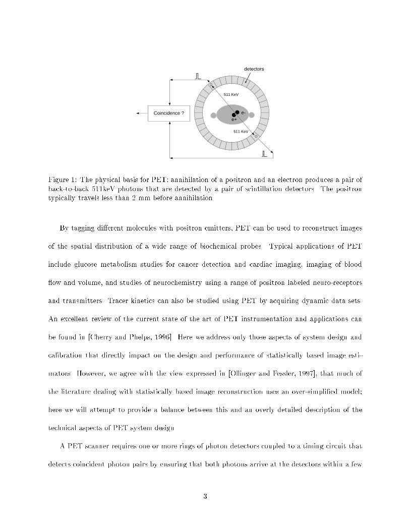
The physical basis for PET imaging lies in the fact that a positron produced by a radioactive nucleus

annihilates with an electron to form a pair of high energy (511keV) photons after traveling a very

short distance. The pair of photons travel back-to-back along a straight line path. Detection of the

positions at which the photon pair intersect a ring of detectors, Fig. 1, allows us to approximately

determine the locus of a line containing the positron emitter. The total number of such events

measured by a pair of detectors will be proportional to the total number of such emissions along

the line joining the detectors. If positron emitters are spatially distributed with density f(x) at

location x, the number of detected events between a pair of detectors is an approximate line integral

through this distribution.

2

Coincidence ? e-e+

511 KeV

detectors

511 KeV

Figure 1: The physical basis for PET: annihilation of a positron and an electron produces a pair ofback-to-back 511keV photons that are detected by a pair of scintillation detectors. The positrontypically travels less than 2 mm before annihilation.

By tagging di�erent molecules with positron emitters, PET can be used to reconstruct images

of the spatial distribution of a wide range of biochemical probes. Typical applications of PET

include glucose metabolism studies for cancer detection and cardiac imaging, imaging of blood

ow and volume, and studies of neurochemistry using a range of positron labeled neuro-receptors

and transmitters. Tracer kinetics can also be studied using PET by acquiring dynamic data sets.

An excellent review of the current state of the art of PET instrumentation and applications can

be found in [Cherry and Phelps, 1996]. Here we address only those aspects of system design and

calibration that directly impact on the design and performance of statistically based image esti-

mators. However, we agree with the view expressed in [Ollinger and Fessler, 1997], that much of

the literature dealing with statistically based image reconstruction uses an over-simpli�ed model;

here we will attempt to provide a balance between this and an overly detailed description of the

technical aspects of PET system design.

A PET scanner requires one or more rings of photon detectors coupled to a timing circuit that

detects coincident photon pairs by ensuring that both photons arrive at the detectors within a few

3

DETECTORS

DETECTORS

DETECTORS

DETECTORS

DETECTORS

(a)

(b)

Figu

re2:

Schem

aticofan

axialcro

sssection

throu

gh(a)

a2-D

and(b)a3-D

PETscan

ner.

The

septa

inthe2D

scanner

stopout-o

f-plan

ephoton

swhile

the3D

scanner

detects

these

events

asaddition

aldata

.

nanoseco

ndsofeach

other.

Auniqueasp

ectofPETas

compared

tomost

othertom

ographicsystem

s

isthatthecom

plete

ringofdetectors

surrou

ndingthesubject

allowssim

ultan

eousacq

uisition

of

acomplete

data

setso

thatnorotation

ofthedetector

system

isreq

uired

.A

schem

aticview

of

twomodern

PETsca

nners

isshow

nin

Figu

re2.

Multip

lerin

gsof

detectors

surrou

ndthepatien

t

with

ringsofdense

material,

or\sep

ta",sep

aratingeach

ring.

These

septa

stopphoton

stravelin

g

betw

eenrin

gsso

thatcoin

cidence

events

arecollected

only

betw

eenpairs

ofdetectors

inasin

gle

ring.

Wewill

referto

thiscon�guratio

nas

a2D

scanner

since

thedata

aresep

arableandtheimage

canbereco

nstru

ctedas

aseries

of2Dsection

s1.

Incon

trast,the3D

scanners

have

nosep

taso

that

coincid

ence

photonscanbedetected

betw

eenplan

es.Thisresu

ltsin

afactor

of4to

7increase

in

thetota

lnumber

ofphoto

nsdetected

andhence

increases

thesign

alto

noise

ratio.In

thiscase

the

reconstru

ctionprob

lemisnot

separab

leandmust

betreated

directly

in3D

.

Inmost

scanners,

thedetecto

rscon

sistof

acom

bination

ofscin

tillatorsandphotom

ultip

lier

1Thispicture

israthersim

pli�

edsin

ce2D

system

sdoallow

detectio

nofevents

betw

eenadjacentrin

gs.

These

are

used

toreconstru

ctadditio

naltra

nsaxialim

ages,

sothatthethick

ness

ofeach

planeishalfoftheaxialexten

tofa

single

detec

torrin

gandthenumberofreconstru

ctedplanes

ina2D

scanner

isusually

2P�1where

Pisthenumber

ofdetec

torrin

gs.

4

Figure 3: Photograph of a block-detector: an 8 by 8 array of BGO crystals are coupled to fourlarger photomultiplier tubes (PMTs). The light output from each crystal is shared between thePMTS; the resulting output signals from the PMTs are used to decide from which crystal this lightoriginated.

tubes (PMTs). Scintillators used in PET include bismuth germinate (BGO), sodium iodide (NaI)

and lutetium oxyorthosilicate (LSO). These convert the high energy 511keV photons into a large

number of low energy photons. These are then collected and ampli�ed by the PMTs. Typically 64

scintillation detectors will be coupled to four PMTs as shown in Fig. 3. The output signal from

all four PMTs is used to determine in which of the 64 crystals the 511 keV photon was absorbed.

Arranging the detector blocks in circular fashion produces a ring scanner; additional rings of blocks

are added to increase the axial �eld of view of the scanner.

With this basic picture of a PET system, we can now turn to the issues of data modeling and

image reconstruction. Consider �rst the 2D arrangement. In the absence of an attenuating medium

and assuming perfect detectors, the total number of coincidences between any detector pair is ap-

proximately a line integral through the 2D source distribution. The set of line integrals of a 2D

function form its Radon transform, thus the coincidence data are readily sorted into a Radon trans-

form or sinogram format as illustrated in Fig. 4. Once the sinogram data have been collected, the

source distribution can be reconstructed using the standard �ltered back-projection algorithm which

5

θ

y

x

u

3 pointsources

u

θ

g(u,θ) = ∫ f(x,y) dv

0 50 100 150 200 250

0

0.5

1

1.5

2

2.5

3

(a) (b)

Figure 4: Coincidence detection between parallel pairs of detectors in (a) corresponds to one lineof the Radon transform of the source distribution in (b). A point source in (a) maps to a sinusoidin Radon transform space (b).

is a numerical method for inverting the Radon transform of a 2D function [Shepp and Logan, 1974].

In the 3D case, the presence of oblique line-integral paths between planes make the analytic

problem less straightforward. Not only is there a huge increase in the amount of data, but also the

limited axial extent of the scanner results in missing data in the oblique sinograms. One solution

to this problem is to use an analytic solution in combination with a reprojection procedure to �ll

in the missing data [Kinahan and Rogers, 1989]. An alternative approach to 3D reconstruction is

to \rebin" the data in to equivalent 2D sinograms and apply 2D reconstruction algorithms to the

result. The cruder forms of rebinning lead to substantial resolution loss, however, recent Fourier

rebinning methods, achieve impressive speed up in computation with little loss in performance

[Defrise et al, 1997].

While the analytic approaches result in fast reconstruction algorithms, accuracy of the recon-

structed images is limited by the approximations implicit in the line integral model on which the

reconstruction formulae are based. In contrast, the statistical methods that we will review here

can adopt arbitrarily accurate models for the mapping between the source volume and the sino-

6

grams. A second limitation of the analytic approaches is that they do not take account of the

the statistical variability inherent in photon limited coincidence detection. The resulting noise in

the reconstructions is controlled, at the expense of resolution, by varying the cut-o� frequency of

a linear �lter applied to the sinogram. Since the noise is signal dependent, this type of �ltering

is not particularly e�ective at achieving an optimal bias-variance trade-o�. Again, the statistical

approaches allow explicit modeling of statistical noise associated with photon limited detection.

The combination of improved modeling of the detection process and improved handling of statis-

tical noise when using statistically based methods, o�ers the possibility for enhanced performance

of PET in both high count data (where model accuracy limits resolution) and low count data (where

statistical noise limits resolution). In its simplest form, the imaging problem can be cast as one

of parameter estimation where the data are Poisson random variables with mean equal to a linear

transformation of the parameters. This formulation is complicated, as we will describe here, by

the impact of additional noise and correction terms. To give an idea of the scale of the problem, a

single 3D scan from the latest generation of PET systems could produce 107-108 sinogram elements

with 106 image elements to be estimated.

We have organized the paper as follows. We �rst develop a model for the PET data based on

the physics of coincidence detection. We then review various formulations of the inverse problem

that derive from the Poisson model for the coincidence data. Here we also address the issue of

ill-posedness and review the various forms of regularization used to overcome it. We then turn

our attention to the wide range of numerical methods for optimizing the chosen cost function. We

conclude with a description of some the recent work in evaluating estimator performance, both in

terms of basic properties such as bias and variance, and also in terms of task speci�c evaluation.

7

2 Data Modeling

2.1 The Coincidence Model

For the purposes of this review, we will assume that the image is represented using a �nite set of

basis functions. While there has been some interest in alternative basis elements, (e.g. smooth

spherically symmetric \blobs" [Matej and Lewitt, 1996]), almost all researchers currently use a

cubic voxel basis function. Each voxel is an indicator function on a cubic region centered at one

of the image sampling points in a 2D or 3D lattice. The image value assigned to each voxel

is proportional to the total number of positron-emitting nuclei contained in the volume spanned

by the voxel. A single index will be used to represent the lexicographically ordered elements of

the image, f = ffj ; j = 1 : : :Ng. Similarly, the elements of the measured sinograms will be

represented in lexicographically ordered form as y = fyi; i = 1; : : :Mg. To give an idea of the size

of the problem, we have listed some of the basic parameters for a 3D whole body PET scanner in

Table 1.

Since the data are inherently discrete and the detection process approximately linear, the map-

ping between the source image and the expected value of the true coincidence data can be repre-

sented by a forward projection matrix, P 2 IRM�N . The elements, p(i; j) contain the probability

of detecting an emission from voxel site j at detector pair i. As we will see below, the measured

data are corrupted by additive random coincidences, r, and scattered coincidences, s, so that the

basic model for the mean of the data is:

�y = E[Y] = Pf + r+ s (1)

The emission of positrons from a large number of radioactive nuclei is well known to follow a

8

ring diameter, mm 413 object size, mm 128 � 128� 63

detectors per ring 576 object size, voxels 128 � 128� 63

number of rings 32 voxel size, mm 2:25� 2:25� 2:43

angles per sinogram 144 full size of P 1013

rays per angle 288 storage size of PGeom 42 Mbytes

number of sinograms 239 storage size of PBlur 0.5 Mbytes

projections per sinogram 41,472 storage size of PAttn and PE� 40 Mbytes

total projection rays 107 total storage size of P 82.5 Mbytes

Table 1: Typical problem dimensions for reconstruction of images from the Siemens/CTI EXACT HR+

body scanner. Use of sparse structures and symmetry reduce the matrix size to manageable proportions.

Poisson distribution. Provided that the detection of each photon pair by the system is independent

and can be modeled as a Bernoulli process, then the sinogram data are a collection of Poisson

random variables. The independence in detection does not strictly hold since all PET scanners are

limited in the rate at which they can count - a restriction re ected in the so-called \dead-time"

calibration factor which is a measure of the fraction of time that the scanner is unable to record

new events because it is processing photons that have already arrived. Here we will assume that

the count rates are su�ciently low that the system is operating in the linear range and the data in

(1) can be well modeled as Poisson with mean y. As we will see later, in most PET scanners the

data are actually pre-corrected for random coincidences

so that they are no longer Poisson. We now consider each the three terms on the right hand

side of (1) and describe how they can be handled within a statistical formulation of the inverse

problem.

2.2 True Coincidences

In an e�ort to develop an accurate and computationally e�cient representation of the projection

data we have developed the following factored representation:

P = Pdet:sensPdet:blurPattnPgeomPpositron (2)

9

While this speci�c factorization has been used only in our own work [Qi et al, 1998], it is a

useful form for describing the various components of the forward projection matrix.

Ppositron: the emitted positron travels a small distance before annihilating with an electron. The

distance is dependent on the speci�c isotope and the density of the surrounding tissue. In water,

the common PET isotopes have full width at half maximum (FWHM) ranges between 0.1mm for

18F to 0.5mm for 15O [Levin et al, 1997]. The range distributions are long tailed so that although

these factors are negligible for 18F studies, they are one of the primary factors limiting resolution

in 15O studies. We can include positron range in the PET data model by making Ppositron a

local image blurring operator that is applied to the true source distribution. If we assume that

the density inside the patient is that of water, then these factors would be shift invariant. More

sophisticated modeling with shift-variant blurs would involve the use of an attenuation map (see

Section 2.3) to determine spatially variant positron range distributions. In most work to date these

factors have not been included in the model, although there have been attempts to de-convolve

these factors from either the sinogram data or the reconstructed image [Haber et al, 1990].

Pgeom: is a matrix that contains the geometrical mapping between the source and data. The (i; j)th

element is equal to the probability that a photon pair produced in voxel j reaches the front faces of

the detector pair i. While the conventional model for this is based on computing the intersection

of a tube joining the detector pair with each voxel, the correct model is actually based on the solid

angle subtended at each of the detectors by each voxel [Qi et al, 1998].

The dominant cost in all iterative PET reconstruction algorithms is that involved in forward

and backward projection. Using the factored form above, the most expensive part of this operation,

is multiplication by Pgeom or its transpose. Consequently, it is very important that this matrix be

represented e�ectively to minimize storage and computation costs. Although Pgeom is extremely

large it is also very sparse with a high degree of symmetry. The sparseness arises from the small

10

fraction of voxels that can produce coincidences at each detector pair. In 2D there is a total of an 8-

fold symmetry in the data for a circular ring of detectors; in 3D there are additional symmetries for

coincidences between detector rings [Johnson et al, 1995, Chen et al, 1991, Qi et al, 1998]. Further

savings in storage costs and computation time can be realized by storing only non-zero elements

and using automated voxel indexing. The reductions that can be achieved are illustrated in Table

1.

Pattn: the geometric term above will determine the number of photons reaching the detectors

only in the absence of an attenuating medium. In fact, the body prevents a substantial fraction

of photons reaching the detectors, primarily through Compton scattering of one or both photons

[Barrett and Swindell, 1981]. It is straightforward to show that the probability of attenuation is

constant for all emissions producing photon pairs that would otherwise impinge on a given detector

pair, so that the attenuation factor can be represented by a diagonal matrix containing the survival

probabilities. Accurate attenuation factors are crucial for obtaining high quality PET images and

we return to this topic in Section 2.3.

Pdet:blur: Once photons arrive at the detectors, the detection process is complicated by a number of

factors which we have lumped into the matrix Pdet:blur that acts as a local blurring function applied

to the sinogram formed by multiplying the source distribution by the geometric projection matrix.

The blurring occurs for three primary reasons: (i) the photons are not exactly co-linear; (ii) photons

may be scattered from one crystal in a detector block to another resulting in a mis-positioning of

the detected photon in the block; (iii) the crystal surface is not always orthogonal to the direction

of arrival of the photon so that a photon may penetrate through one or more crystals before being

stopped. These factors are illustrated in Figure 5. In principle the non-colinearity e�ect should

have been combined with the geometric matrix, but we have found that it can be included in the

blurring factors without noticeable loss in model accuracy. Exact computation of the three factors

11

e-

e+e-

e+

e-

e+

(a) (b)

e-

e+

e-

e+

(c) (d)

Figure 5: Figure shows various factors that complicate the basic PET model: (a) scatter withinthe body) (b) random coincidences (c) inter-crystal scatter (d) crystal penetration.

is not practical. Instead we have used Monte Carlo simulations in which we track large numbers

of photon pairs through a simpli�ed model of the detectors [Mumcuoglu et al, 1996b]. As with the

geometric matrix, there is a great deal of symmetry in these blur factors. Furthermore the blurring

extends over a small area of the sinogram so that storage and computation costs associated with

these factors are small. By factoring these e�ects out of the geometric projection matrix we achieve

a reduction by a factor of approximately three in the geometric matrix size and comparable savings

in reconstruction time.

Pdet:sens: Once a photon pair reach a given detector the event may not be detected since no detector

is 100 % e�cient. Pdet:sens is again a diagonal matrix which contains the detector e�ciency factors.

The terms that contribute to these factors include the intrinsic sensitivities of the individual crystals,

the relative position of the crystals within a detector block, and geometric factors related to the

12

distance of the detector pair from the center of the �eld of view [Casey et al, 1995]. An additional

complicating factor is that of system dead-time which is an approximate measure of the fraction of

counts lost due to the detectors being unable to detect new photons since the system is occupied

with events that were previously detected. These factors are all measured through calibration

procedures and are typically provided to the user in a form that can be used to directly generate

a normalization or diagonal Pdet:sens matrix. However, a word of caution is appropriate since the

dead-time factor does cause non-linear behavior at high count rates and methods to account for

this are still needed.

2.3 Attenuation E�ects

A substantial fractions of the photons emitted through positron-electron annihilation do not directly

exit the body. Rather they undergo Compton scattering [Barrett and Swindell, 1981] in which the

energy of the photon is reduced and its direction is altered. If this photon is later detected, then a

scattered event is recorded as discussed below. Whether or not the scattered photon is detected,

there is a net loss of counts along the original path on which the photon pair was traveling. It is

straightforward to show, under the line integral model, that the probability of attenuation along

any straight line path is independent of the location along the path that the original annihilation

occurs. The survival probability for a photon pair is equal to expf�R�(x)dlg, where �(x) is the

linear attenuation coe�cient at x and the integral is taken along the straight line path.

In most instances the attenuation factor is found using an external transmission source. These

sources are usually either a ring of positron emitting material that surrounds the patient, or a rotat-

ing rod of activity. Photons traveling along straight line paths through the patient are attenuated

according to the same probability as emitted photons within the body that are traveling on the

same paths. A simple estimate of the probability of survival can be computed as the ratio of the

13

number of photon pairs detected with the patient present (the transmission scan) to the number

detected in the absence of the patient or attenuating medium (the blank scan).

This simple division method of computing survival probabilities produce high variance and bi-

ased estimates. Errors are particularly large when the number of detected transmission counts is

low. Alternatively, the transmission data can be used to reconstruct an image of the linear atten-

uation coe�cients via statistical methods very similar to those reviewed below. As with emission

data, the transmission scans are photon limited and contain scattered and random coincidences.

Formulation of the transmission reconstruction problem follows in a similar manner to the emission

methods described here, with the primary di�erent being that the mean of the data contain the line

integrals of the attenuation image in exponential form. Rather than pursue this issue further here,

we refer the interested reader to [Lange et al, 1987, Fessler et al, 1997, Mumcuoglu et al, 1994].

2.4 Random and Scattered Coincidences

The true coincidence data are corrupted by two forms of additive noise. These are the scatter and

randoms components, s and r respectively, in (1). Scattered events refer to coincidence detection

after one or both of the photons has undergone Compton scattering. Clearly, after scattering, we

can no longer assume that positron emission occurred along the path joining the two detectors.

Scattered photons have lower energy than their unscattered 511keV counterparts. Consequently

some of the scattered events can be removed by rejecting events for which the energy detected by

the PMTs does not exceed some reasonable threshold. Unfortunately, setting of this threshold

su�ciently high to reject most of the scattered radiation will also result in rejection of a large

fraction of unscattered photons. For the most commonly used BGO detectors with the standard

energy thresholds, 2D PET studies typically have a scattered to true coincidence ratio of about

10% while in 3D studies the fraction often exceeds 30%. Typically scatter contributions to the data

14

tend to be fairly uniform. They are often simply ignored in qualitative studies since they result

in an approximately constant o�set in the image when using linear estimators. When non-linear

methods are used or when accurate quantitation is required, these factors must be modeled.

Given the distribution of the source image and an image of the linear attenuation coe�cient,

an accurate scatter pro�le can be computed using the Klein-Nishina formula for Compton scat-

ter [Barrett and Swindell, 1981]. Since the scatter pro�les are smooth, it is possible to compute

them with reasonable computational load from a low resolution, preliminary reconstruction of the

emission source. Once this is estimated, the scatter contribution can be viewed as a known o�-

set in the mean of the data in (1) rather than as an explicit function of the data that must be

re-computed with each new estimate of the image. Model based scatter methods are described in

[Ollinger et al, 1992, Watson et al, 1995, Mumcuoglu et al, 1996a]. In the following we will assume

that the scatter component in the data has been estimated using one of these methods.

Random coincidences, as mentioned above, are caused by the detection of two independent

photons within the coincidence timing window. The randoms contribution to the data is a function

of the length of this timing window and of the source activity. By simply delaying the timing

window by a �xed amount, one can obtain data which is purely randoms and with the same mean

number of counts as for the non-delayed window. Thus on most scanners, a randoms corrected data

set is collected in which two timing windows are used, one to collect true and randoms, the second

to just collect randoms. The di�erence of these two is the corrected data. While this does correct

the data, in mean, for the randoms, the resulting data has increased variance due to the subtraction

of two Poisson processes. This has important implications for the data model as discussed below.

15

3 Formulating the Inverse Problem

3.1 Likelihood Functions

The great majority of publications employing statistical PET models assume the data y is Poisson

with mean �y and distribution

p(yjf) =MYi=1

�yiyie� �yi

yi!(3)

The corresponding log-likelihood is

L(yjf) =MXi=1

�yi log yi � �yi (4)

The mean �y is related to the image through the a�ne transform (1). In most cases, the e�ects

of scatter and randoms, whether present or subtracted from the data, are simply ignored and the

data are assumed to follow this Poisson model with mean �y = Pf .

In an e�ort to reduce computation costs and numerical problems associated with the logarithm

that occurs in the log-likelihood function, [Fessler, 1994] and [Bouman and Sauer, 1996] suggest

using a quadratic approximation to the data:

L(yjf) = �1

2

MXi=1

( �yi � yi)2

�2i(5)

where � is some estimate of the variance of each measurement, typically this is set equal to the

observed data. Using this approximation, maximum likelihood reduces to weighted least squares.

However, such a crude estimate of the variance inevitably leads to degradation in performance.

Using a constant variance for all data reduces the problem to conventional least squares which

16

produces higher variance than the weighted least squares method.

The Poisson model above is appropriate only when the data have not been corrected for randoms,

and when the randoms and scatter components are explicitly included in the model. When operated

in standard mode, PET scanners pre-correct for randoms by computing the di�erence between

coincidences collected using a standard timing window and those in a delayed timing window. These

data are Poisson processes with means y = E[y] = Pf + r+ s and r, respectively. The precorrected

data y has mean Pf + s and variance Pf + 2r+ s so that a Poisson model does not re ect the true

variance. The true distribution has a numerically intractable form and an approximation should

be used [Yavuz and Fessler, 1996]. One possibility is to modify the quadratic approximation in (5)

using an increased variance. A better approximation is the shifted-Poisson model in which the �rst

two moments of the corrected data are matched by assuming that y + 2r is Poisson with mean

Pf + 2r+ s. This results in the modi�ed log likelihood:

L(yjf) =MXi=1

( �yi + 2ri) log((Pf)i + 2ri + si)� ((Pf)i + 2ri + si) (6)

In closing this section we note that likelihood functions that model the increase in variance due

to randoms subtraction need estimates of the mean of this randoms process. These must in turn

be estimated from the measurements and calibration data [Fessler, 1994, Qi et al, 1997].

3.2 Priors

Direct maximum likelihood (ML) estimates of PET images exhibit high variance due to ill-conditioning.

Some form of regularization is required to produce acceptable images. Often this is accomplished

simply by starting with a smooth initial estimate and terminating an ML search before conver-

gence. Here we consider explicit regularization procedures in which a prior distribution is intro-

17

duced through a Bayesian reformulation of the problem to resolve ambiguities in the likelihood

function. Some authors prefer to present these regularization procedures as penalized ML methods

but the di�erences are largely semantic, except in the case where the penalty functions are explicit

functions of the data, e.g. [Fessler and Rogers, 1996].

Bayesian methods can address the ill-posedness inherent in PET image estimation through the

introduction of random �eld models for the unknown image. In an attempt to capture the locally

structured properties of images, researchers in emission tomography, and many other applications of

image processing, have adopted Gibbs distributions as suitable priors. The Markovian properties of

these distributions make them theoretically attractive as a formalism for describing empirical local

image properties, as well as computationally appealing since the local nature of their associated

energy functions result in computationally e�cient, update strategies.

The Gibbs distribution has the general form

p(f j�) =1

Ze��U(f) (7)

where U(f) is the Gibbs energy function de�nes as a sum of potentials, each of which is a function of

a subset or clique ck � S where S = f1; 2; : : :Ng is the set of image voxels. The Gibbs distribution

is de�ned on a neighborhood system which associates a set of sites Wi � S with each site i. The

neighbors of each site are typically the collection of pixels closest, up to some maximum Euclidean

distance, to site i. To be a true Gibbs distribution, each pair of sites in each clique ck must be

mutual neighbors.

The form of Gibbs distributions most commonly used in image processing are those for which

18

the energy function U(f) contains potentials de�ned only on pair-wise cliques of neighboring pixels:

U(f) =NXj=1

Xk2Wi;k>j

�jk(fj � fk) (8)

For a 3D problem, the neighbors of an internal voxel would be the nearest 6 voxels for a 1st order

model, or the nearest 26 voxels for a 2nd order model (with appropriate modi�cations for the

boundaries of the lattice).

The potential functions �jk(fj � fk) are chosen to attempt to re ect two con icting image

properties: (i) images are typically piecewise smooth, (ii) except where they are not! For example,

in PET images we might expect to see smooth variations in tracer uptake within a speci�c organ

or type of tissue, and abrupt changes as we move between di�erent organs or tissue types. A wide

range of functions have been studied in the literature that attempt to produce local smoothing while

not removing or blurring true boundaries or edges in the image. All have the basic property that

they are monotonic non-decreasing functions of the absolute intensity di�erence j(fj� fk)j. Taking

the square of this function leads to a Gauss-Markov prior which produces smooth images with

very low probability of sharp transitions in intensity. In an attempt to increase the probability of

these sharp transitions, [Bouman and Sauer, 1996] propose using the generalized p-Gaussian model

where �(f) = jf jp, 1 < p < 2. An alternative function with similar behavior, that derives from

the literature on robust estimation, is the Huber prior in which �(f) transitions from quadratic to

linear at a user speci�ed transition point. Both of these examples produce convex energy functions.

In an attempt to produce even sharper intensity transitions, several highly non convex functions

have also been proposed. For example, [Geman and McClure, 1985], who were also the �rst to

speci�cally use Gibbs distributions in emission tomography, proposed the function �(f) = f2

f2+�2.

This and other non-convex potentials have the property that the rate of increase of the function

19

decreases as the intensity di�erence increases. The limiting case of this approach is found in the

weak membrane model which is quadratically increasing up to some threshold and then remains

constant beyond this [Gindi et al, 1993].

Higher order neighborhoods are able to capture more complex correlation structure than the

simple pair-wise models [Chan et al, 1995]. Unfortunately, the problem of choosing, and justifying

such a model becomes increasingly di�cult with the size of the neighborhood. One example which

was used to nice e�ect, is the thin plate model of [Lee et al, 1995]. This model uses a discrete

approximation to the bending energy of a thin-plate as the Gibbs energy function. Since the thin

plate energy involves second order derivatives, higher order cliques must be used in the model.

Rather than implicitly model image boundaries, compound MRFs model them explicitly using

a second coupled random �eld de�ned on a dual lattice. The dual lattice points are placed between

each pair of sites in the image lattice and are set to unity if there is an image boundary between

that pair of voxels, otherwise they are set to zero. In this way, the prior can explicitly model edges

in the image, and introduce additional potential terms to encourage the formation of connected

boundaries [Geman and Geman, 1984]. A wide range of compound MRFs have been studied in the

PET literature, .e.g. [Lee et al, 1995, Johnson et al, 1991, Leahy and Yan, 1991].

One of the primary attractions of the compound MRFs is that they serve as a natural framework

for incorporating anatomical information into the reconstruction process [Leahy and Yan, 1991,

Gindi et al, 1991, Gindi et al, 1993]. Since di�erent anatomical structures have di�erent physiolog-

ical functions, we can expect to see di�erences in tracer uptake between structures. This general

observation is borne out in high resolution autoradiographic images in which functional images also

clearly reveal the morphology of the underlying structures [Gindi et al, 1993]. Because the anatom-

ical modalities, such MR and CT, have superior resolution and SNR, fairly accurate location of the

boundary process can be formed, these can then be used to in uence the formation of the boundary

20

process in the PET image estimation procedure.

3.3 The Posterior Density

The likelihood function and image prior are combined through Bayes rule to produce the posterior

density

p(f jy) =p(yjf)p(f)

p(y): (9)

Images can be computed using either maximum a posteriori (MAP) estimation (MAP) or some

other loss function. Computation of anything but the MAP estimate is often impractical, but see

[Bowsher et al, 1996] for an example of a hierarchical MRFmodel for emission tomography in which

MAP estimation is not used. In the following we will consider only MAP estimation procedures.

Taking the log of the posterior and dropping constants, we have the basic form of the MAP

objective function

�(f ;y) = L(yjf)� �U(f): (10)

Since the log likelihood functions in Section 3.1 are convex, the convexity of the objective function is

determined by the prior. If compound MRFs are used, or simple MRFs with non-convex potentials,

there will exist multiple local maxima. In these cases, special care is initializing a local search

algorithm. Furthermore, the inherent discontinuity of the solution with respect to the data can

result in unpredictable behavior resulting, in some case, in high variance estimates.

21

4 Image Estimation

4.1 ML Estimators

Because of the complexity and high dimensionality of the log likelihood function, ML solutions

are computed iteratively. Iterative estimation schemes in PET have their basis in the row-action

or ART (algebraic reconstruction techniques) developed during the 1970s [Censor, 1983]. ART

solves a set of linear equations by successive projection of the image estimate onto the hyperplanes

de�ned by each equation. The approach is attractive for the sparse matrix structures encountered

in PET but has no statistically optimal properties. In cases where the data are consistent, ART will

converge to a solution of these equations, but in the inconsistent case, the iterations will continue

inde�nitely. Many variations on this theme can be found in the literature [Censor, 1983] but we

will restrict attention here to estimators that are based on explicit statistical data models.

[Rockmore and Macovski, 1976] published an early paper on ML methods for emission tomog-

raphy, but it was the work of [Shepp and Vardi, 1982] and [Lange and Carson, 1984], who applied

the EM algorithm of [Dempster et al, 1977] to the problem, that lead to the current interest in ML

approaches for PET. In large part, the attraction of this method to the nuclear medicine commu-

nity, is that the EM methods produces an elegant closed-form update equation reminiscent of the

earlier ART methods.

The EM algorithm is based on the introduction of a set of complete but unobservable data, w,

which relates the incomplete observed data y to the image f . The algorithm alternates between

computing the conditional mean of the complete data log likelihood function, ln p(w; f), from y

and the current image estimate, f (k), and then maximizing this quantity with respect to the image,

22

i.e.:

E � step : Q(f ; f (k)) = E[lnL(w; f)jy; f (k)]

M � step : fk+1 = argmaxf Q(f ; f(k))

(11)

For the PET reconstruction problem the complete data is chosen as w = ffwijgNj=1g

Mi=1 with each

wij denoting the emissions from voxel j being detected by detector pair i [Lange and Carson, 1984].

In this model, random and scatter are ignored but modi�cations to deal with these as additive

factors are straightforward. The �nal EM algorithm has the form:

E � step : Q(f ; f (k)) =P

j(f(k)

j

Pi

pijyi

(P

lpilf

(k)

l)log(pijfj)� fj

Pi pij)

M � step : f(k+1)

j =f(k)

jPipij

Pi

pijyiPlpilf

(k)

l

(12)

Two problems were widely noted with this algorithm: it is slow to converge and the images

have high variance. The variance problem is inherent in the ill-conditioning of the objective func-

tion. In practice it is controlled in EM implementations using either stopping rules, i.e. stopping

before convergence [Veklerov and Llacer, 1987, Coakley, 1991, Johnson, 1994] or post-smoothing of

the reconstruction [Llacer et al, 1993, Silverman et al, 1990]. An alternative approach to avoiding

instability is to used Grenander's method of sieves [Grenander, 1981]. The basic idea is to maximize

the likelihood over a constrained subspace and then relax the constraint by allowing the subspace

to grow with the sample size. This usually produces consistent estimates provided that the sieve

grows su�ciently slowly with sample size. [Snyder and Miller, 1985] have successfully applied this

approach to PET using a Gaussian convolution-kernel sieve.

Many researchers, [Lewitt and Muehllehner, 1986, Kaufman, 1987, Rajeevan et al, 1992], have

23

studied methods for speeding up the EM algorithm by re-writing the EM update equation as:

f(k+1)

j = f(k)

j + f(k)

j

1Pi pij

@L(yjf (k))

@fj: (13)

Re-written in this way, EM looks like a special case of gradient ascent and some degree of speed-up

can be realized using over-relaxation or line-search methods. More substantial gains are achieved

by returning to standard gradient ascent methods, and in particular pre-conditioned conjugate

gradient searches [Kaufman, 1993].

One distinct attraction of the original EM algorithm is that the updates impose a natural

non-negativity constraint. This is not shared by the gradient-based methods and imposition of

a positivity condition on these methods requires careful handling [Kaufman, 1993]. An alterna-

tive to gradient based searches is to use iterated coordinate ascent (ICA) methods in which the

voxels are updated sequentially, thus making imposition of the non-negativity constraint trivial.

ICA also leads to dramatic speed up in convergence rate in comparison to the EM algorithm

[Bouman and Sauer, 1993]. We will return to gradient based and ICA approaches in our discussion

of regularized methods.

The ordered subsets EM (OSEM) [Hudson and Larkin, 1994] is a modi�cation of the EM algo-

rithm in which each update only uses a subset of the data. Let fSigpi=1 be a disjoint partition of

the integer interval [1;M ] =Spi=1 Si. Let k denotes the index for a complete cycle and i the index

for a sub-iteration, and de�ne f (k;0) = f (k�1),f (k;p) = f (k). then the update equation for OSEM is

given by

f(k;i)

j =f(k;i�1)j

cij

Xi2Si

pijyiPl pilf

(k;i�1)

l

; for j = 1; � � � ; N: i = 1; � � � ; p: (14)

where cij =P

i2Sipij . An earlier example of iterating over subsets of the data for ML estimation in

24

emission tomography can be found in [Hebert et al, 1990]. OSEM produces remarkable improve-

ments in convergence rates in the early iterations, although subsequent iterations over the entire

data is required for ultimate convergence. If the number of subsets remains greater than one, then

OSEM will enter a limit cycle condition [Byrne, 1997]. Several variations on the OSEM algorithm

have been proposed. One of the more interesting is the row-action maximum likelihood algorithm

of [Browne and De Pierro, 1996]. This is similar to OSEM, but can be shown to converge to a true

ML solution under some conditions. As with the original EM algorithm, OSEM produces high

variance at large iteration numbers. This is typically controlled using either early termination or

post smoothing of the image. Although OSEM does not converge in general, it is currently the most

widely used iterative method for statistically based reconstruction in emission tomography. This is

primarily due to the obvious improvements in image quality over standard �ltered back-projection

methods couple with the relatively low computational cost involved in using this method.

While the EM and OSEM methods were originally derived for the pure Poisson model, modi�-

cations for the case of an o�set due to randoms and scatter or increase in variance due to randoms

subtraction have also been developed.

4.2 Bayesian Methods and other forms of Regularization

The EM algorithm can be directly extended to include prior terms by using the generalized EM

method [Dempster et al, 1977, Hebert and Leahy, 1989]. The treatment of the complete data re-

mains the same as for EM-ML, so that the E-step given in (12) does not change. With the addition

of the prior, the M-step must now maximize the log posterior given the complete data, w, i.e.

M � step : fk+1 = argmaxfP

j

�f(k)

j ej(f(k)) log(pijfj)� fj

Pi pij

�� �U(f) (15)

25

where ej(f(k)) =

Pi pijyi=(

Pl pilf

(k)

l )(f (k)). Di�erentiating and setting the result to zero gives the

necessary condition:

f(k)

j ej(f(k))

fj�Xi

pij � �@

@fjU(f) = 0 (16)

Direct solutions of (16) exist only for priors, such as the gamma prior [Lange et al, 1987] [Wang and Gindi, 1997],

in which the voxels are statistically independent. For the case where voxels are not independent, a

gradient search can be applied to the optimization subproblem in (16) [Hebert and Leahy, 1989].

[Green, 1990] proposed a \one-step-late" (OSL) approximation to solve (16). The partial deriva-

tives of U(f) evaluated at the current estimate f (k), resulting in the simple update equation

f(k+1)

j =f(k)

jPi pij + � @

@fjU(f)jf=f (k)

ej(f(k)): (17)

Unfortunately, this procedure does not guarantee convergence to a MAP solution. [De Pierro, 1995]

used a functional substitution method to obtain a closed form update for the M-step. The objective

function was approximated locally by a separable function at current estimate f (k), so that the M-

step involves only a one dimensional maximization which can be solved analytically or using a

Newton-Raphson method. This technique has provable convergence.

The GEM algorithm is readily modi�ed for use with compound MRFs. In that case a set

of binary line site variables must also be estimated. These variables are appended to the set of

parameters to be estimated in the M-step. Since these variables are binary, standard gradient

optimization cannot be applied in the M-step. Instead, mean �eld annealing methods can be used

to estimate the binary variables [Yan and Leahy, 1991, Gindi et al, 1991].

An alternative to the GEM algorithm is the space-alternating generalized EM (SAGE) method

26

[Fessler and Hero, III, 1995]. Unlike the EM algorithms which update image voxels simultane-

ously, SAGE updates image voxels sequentially using a sequence of small \hidden" data spaces.

Because the sequential update decouples the M-step, the maximization can usually be performed

analytically. Since informative complete data spaces slow convergence of EM algorithms, hidden

data spaces that are less informative than those used for ordinary EM, are used to accelerate the

convergence rate yet maintain the desirable monotonicity properties of EM algorithms.

Attempts to produce faster convergence have involved returning to more generic optimiza-

tion techniques based either on gradient or coordinate-wise ascent. The gradient ascent methods

[Kaufman, 1987, Mumcuoglu et al, 1996a, Fessler and Ficaro, 1996] employing preconditioners and

conjugate gradients can give very fast convergence. They are also easily extended to include estima-

tion of line processes using mean �eld annealing methods (MumcuogluLeahyTMI94,BilbroSnyder92).

A major problem in using gradient-based methods is the incorporation of the non-negativity

constraint. Attempts to address this problem include using restricted line searches [Kaufman, 1987],

bent line searches [Kaufman, 1987], penalty function methods [Mumcuoglu et al, 1994] and active

set approaches [Kaufman, 1993].

The non-negativity constraint is more easily dealt with using coordinate-wise updates [Fessler, 1994]

[Bouman and Sauer, 1996, Sauer and Bouman, 1993]. While there are a number of variations on

this basic theme, the essence of these methods is to update each voxel in turn so as to maximize

the objective function with respect that voxel. Given the current estimate f (k), the update for the

jth voxel is

f(k+1)

j = argmaxx�0

[L(yjf)� �U(f)]

����f=ff (k+1)1 ;f(k+1)

2 ;���;f(k+1)

j�1;x;f

(k)

j+1;���;f

(k)

Ng

(18)

To solve the 1D maximization problem, polynomial approximations of the log likelihood function

27

can be used to reduce the update step to closed form [Fessler, 1995]. The Newton-Raphson method

can be used for the general case [Bouman and Sauer, 1996]. These methods can easily incorporate

the non-negativity constraint and achieve similar, or faster, convergence rates to preconditioned

conjugate gradient (PCG) methods.

The computational cost of statistical reconstruction methods are primarily determined by the

number of iterations required, and the number of forward and backward projection operation

required per iteration. The ICA methods of [Bouman and Sauer, 1996] needs one forward and

two backward projection operations, while PCG methods generally only need one forward and

one backward projection operation per iteration. To e�ciently implement ICA algorithms, the

projection matrix needs to be stored in a voxel-driven format. However, it is easier to achieve

e�cient storage of the projection matrix described in Section 2 using a ray-driven format, which

is more suitable for gradient based methods. Partitioning the updates among multiple processors

is also more straightforward for the gradient based methods than ICA. Both methods produce

subsantially faster convergence than the EM algorithm and have the advantage over the OSEM

method that they are stable at higher iterations so that selection of the stopping point of the

algorithm is not critical.

4.3 Parameter Selection

A key problem in the use of regularized or Bayesian methods is the selection of the regularization

parameters, or equivalently the hyperparameters of the prior. MAP estimates of the image f

computed from (10) are clearly functions of � which controls the relative in uence of the prior and

that of the likelihood. If � is too large, the prior will tend to have an over-smoothing e�ect on the

solution. Conversely, if it is too small, the MAP estimate may be unstable, reducing to the ML

solution as � goes to zero.

28

Data-driven selection of the hyperparameter is often performed in an ad hoc fashion through

visual inspection of the resulting images. There are two basic approaches for choosing � in a more

principled manner: (i) treating � as a regularization parameter and applying techniques such as

generalized cross validation, the L-curve, and �2 goodness of �t tests; (ii) estimation theoretic

approaches such as maximum likelihood (ML).

The generalized cross-validation (GCV) method [Craven and Wahba, 1979] has been applied

in Bayesian image restoration and reconstruction [Johnson, 1991]. Several di�culties are asso-

ciated with this method: the GCV function is often very at and its minimum is di�cult to

locate numerically [Varah, 1983]. Also the method may fail to select the correct hyperparameter

when measurement noise is highly correlated [Wahba, 1990]. For problems of large dimensional-

ity, this method may be impractical due to the amount of computation required. Hansen and

Leary's L-curve is based on the empirical observation that the corner of the curve corresponds to

a good choice of � in terms of other validation measures [Hansen, 1992]. The L-curve has simi-

lar performance to GCV for uncorrelated measurement errors, however, the L-curve criterion also

works, under certain restrictions, for correlated errors [Hansen, 1992]. The corner of the L-curve

is di�cult to �nd without multiple evaluations of the MAP solution for di�erent hyperparameter

values. Thus the computation cost is again very high. �2 statistics have been widely used to

choose the regularization parameter [Thompson et al, 1991]. For MAP image estimation, Hebert

et al [Hebert and Leahy, 1992] developed an adaptive scheme based on a �2 statistic to select �.

Since the image is estimated from the data, the degrees of freedom of the test should be reduced

accordingly. This presents a problem when the data and image are of similar dimension. It has

also been observed that �2 methods tend to over-smooth the solution [Thompson et al, 1991].

As an alternative to the regularization based methods discussed above, a well grounded approach

to selection of the hyperparameter is to apply ML estimation. The image f , which can be viewed as

29

a sample drawn from the complete data space F characterized by the parameter �, is not observed

directly. Instead, we observe a second process y which is drawn from the incomplete data sample

space Y . The ML estimate of the hyperparameter corresponds to the maximizer of the incomplete

data likelihood function P (yj�), which is found by marginalization of the joint probability density

for the complete and incomplete data, P (f ;yj�), over the complete data sample space. Selection of

the hyperparameter can therefore be viewed as a ML estimation problem in an incomplete/complete

data framework and is a natural candidate for the EM algorithm [Dempster et al, 1977]. However,

in most imaging applications, the high dimensionality of the densities involved make the EM ap-

proach impractical.

Markov chain Monte Carlo (MCMC) methods [Besag et al, 1995] have been used to evaluate

the E-step of the EM algorithm by some researchers [Geman and McClure, 1987, Zhang et al, 1994,

Saquib et al, ]. [Geyer and Thompson, 1992] propose a Monte Carlo maximum likelihood method

which uses MCMC to approximate the likelihood function directly. [Higdon et al, 1997] developed a

scheme for sampling the posterior distribution, which includes a parameter estimation as part of the

MCMC sampling procedure.This method updates the image and hyperparameters through a joint

posterior distribution.While MCMC methods provide a means for overcoming the intractability of

ML parameter estimation, the computational costs are extremely high.

Other estimation methods have been studied which do not share the desirable properties of

true ML estimation but have much lower computational cost. Several generalized maximum like-

lihood approaches have been described [Besag, 1986, Lakshmanan and Derin, 1989] that make the

simplifying approximation that the ML estimate of � and the MAP estimate of the image f can

be found simultaneously as the joint maximizers of the joint density of f and y. This approach

works well in some situations, but the crudeness of the approximation results in poor performance

in general. The method of moments (MOM) [Geman and McClure, 1987, Manbeck, 1990] de�nes

30

a statistical moment of the incomplete data that is ideally chosen to re ect the variability in the

unobserved image and to establish a one-to-one correspondence between the moment value and the

global hyperparameter. The moment versus hyperparameter curve is independent of the observed

data and can be computed o�-line. For each new data set the hyperparameter is determined by

simply comparing the computed statistic with the precomputed curve. The major limitation in

using this method is in �nding a statistic with su�cient slope that the hyperparameter can be reli-

ably determined. In practice it has been observed that the method performs well only for relatively

small values of � [Manbeck, 1990].

[Zhou et al, 1997] developed an approximation for ML approach based on mean �eld approx-

imation. Gibbs distributions of prior and posterior were approximated by simple and separable

densities so that the multidimensional integrals become functions of one dimensional integrals.

This approximation renders the ML approach tractable. Further, they use a mode-�eld rather

than a mean-�eld approximation, where the mode of the posterior density is computed using a

MAP image estimation algorithm. Successive iterates of a MAP image estimation algorithm are

substituted in the mode-�eld approximation, which in turn is used to update the hyperparameter

estimate.

An interesting alternative to these estimation based approaches to parameter selection, is to

make the parameter user selectable. This is analogous to the case in �ltered backprojection image

reconstruction where the user selects a �lter cut-o� frequency to choose image resolution and hence

e�ect a trade-o� between bias and variance. When combined with the method for uniform resolution

discussed below [Fessler and Rogers, 1996], one can build an object independent table relating the

prior parameter to spatial resolution of the resulting image. The parameter can then be selected

for the desired spatial resolution by the user.

31

5 Examining Estimator Performance

5.1 Resolution

Shift invariant linear imaging systems are often characterized by their point spread function (PSF).

Noiseless data from a point source will produce an image of the PSF so that measurement of the

full-width-at-half-maximum (FWHM) of the PSF is a measure of system resolution. This measure

is useful for images reconstructed using �ltered backprojection since the resulting image resolution

is approximately shift invariant. For non-linear estimators however, PSFs are spatially variant

and object dependent. Therefore, the PSF can only be examined locally and with a speci�c ob-

ject. The local impulse response [Stamos et al, 1988, Fessler and Rogers, 1996] or an e�ective local

Gaussian resolution [Liow and Strother, 1993] can be used to quantify the resolution properties of

the statistical reconstructions.

It is interesting to note that the use of regularizing functions or priors in (10) for PET im-

age estimation will produce spatially variant resolution [Fessler and Rogers, 1996]. These authors

propose a data dependent quadratic penalty function from which a nearly uniform local impulse

response can be obtained. As mentioned in Section 4.3, this spatially-invariant property enables

the selection of a \hyperparameter" based on the desired image resolution. In this case, (10) cannot

be viewed as a true posterior density since the prior term is data dependent.

5.2 Estimator Bias and Variance

For the case of linear methods, closed-form expressions of estimator bias and variance are easily

derived [Barrett, 1990]. Derivations for the case of non-linear estimators is substantially more

di�cult. Monte Carlo studies can always be used to study the performance of any of the estimators

and algorithms discussed above. This approach has been widely used to explore bias-variance trade-

32

o�s in iterative algorithms [Carson et al, 1994]. More recently there has been great progress in the

development of approximate analytic expressions for estimator bias and variance which makes it

practical to explore algorithm behavior in a far more e�cient manner.

An important advance was made by [Barrett et al, 1994] who derived formulae for computing

the �rst and second order statistics for the ML EM algorithm as a function of the iteration. They

showed that the distribution of the kth iteration, f (k), can be approximated by a multivariate

log-normal law with mean and variance

E[f (k)jf ] � �f (k); (19)

K(k)

f (k)� diag(�f (k))U(k)diag(Pf)[U(k)]Tdiag(�f (k)) (20)

where �f (k) is the result of the kth iteration applied to noise-free data, U(k) is an N �M matrix

satisfying the recursion

U(k+1) = B(k) + [I�A(k)]U(k) with U(0) = 0; (21)

with B(k) and A(k) de�ned by

B(k) = diag(1Pi pij

)PTdiag(1

Pj pij

�f(k)

j

] (22)

A(k) = diag(1Pi pij

)PTdiag(1

Pj pij

�f (k)j

]Pdiag(�f (k)): (23)

These results agreed well with Monte Carlo studies for the lower iterations and high projection

count levels [Wilson et al, 1994]. In the limit k !1, where f (k) approaches the ML estimate of f ,

33

the variance of the nth pixel is

var[f (1)n jf ] = [a(1)

n ]2Xm

�h[A(1)]�1B(1)

inm

�2[Pf ]m: (24)

The presence of [A(1)]�1 indicates large noise ampli�cation if the EM algorithm is allowed to run

to large iteration numbers.

Recently, [Wang and Gindi, 1997] made a further advance by extending this analysis to a subset

of the MAP-GEM algorithms. The procedure requires that a closed form update is available, so

the method was applied to the GEM algorithm with an independent gamma prior and to the OSL

algorithm with a class of multivariate Gaussian priors. Using similar approximations to those in

[Barrett et al, 1994], similar expressions for noise propagation were derived with the e�ect of the

prior re ected in the update equation for U in (21).

The main limitation of these methods is that explicit update equations are required. A larger

class of algorithms for PET estimation have implicitly de�ned solutions which require numerical

procedures such as line searches at each iteration. To derive the statistics of these estimators,

[Fessler, 1996] studied the behavior at �xed points of the iterations. The objectives must satisfy

certain di�erentiability criteria, and have a unique, stable �xed point which can be found as the

point where the partial derivatives are zero. As a result, inequality constraints and stopping

rules are precluded. Fortunately, the nonnegativity constraints in PET image reconstruction do

not have much e�ect at the nonzero pixel locations, so the mean and variance approximations

for an unconstrainted estimator may agree closely with the actual performance of an estimator

implemented with nonnegativity constraints [Fessler, 1996].

By using the �rst-order Taylor series approximation of the estimator at the �xed point, f , of

34

the objective function, the mean and covariance of f can be approximated as:

Effg � �f

K(k)

f (k)� [�r20�(�f ; �y)]�1r11�(�f ; �y)Covfyg[r11�(�f ; �y)]T [�r20�(�f ; �y)]�1;

(25)

where �f is the reconstruction of noise-free data. Covfyg is the covariance matrix of the data,

the (j; k)th element of the operator r20 is @2

@fj@fk, and the (j; n)th element of the operator r11 is

@2

@fj@yn. Note that (25) is independent of the particular algorithm used to optimize the objective.

Comparison of these formulae with results of Monte Carlo studies showed generally good agreement

except in regions of very low activity.

[Hero et al, 1996] proposed an alternative to explore estimator bias-variance tradeo�s using the

uniform Carmer-Rao (CR) bound. They introduce a delta-sigma plane, which is indexed by the

norm of the estimator bias gradient and the variance of the estimator. The norm of the bias

gradient is related to the maximum variation in the estimator bias function over a neighborhood

of the parameter space. The larger the norm of the bias gradient, the larger the uncompensatable

bias the estimator will have. Using a uniform CR bound on the estimator variance, a delta-

sigma tradeo� curve, which de�nes an unachievable region on the delta-sigma plane for a speci�ed

statistical model, can be generated. This delta-sigma tradeo� curve can then be used to compare

di�erent statistical models and also to assess the estimator performance.

In Fig. 6 we show an example of computing bias and variance for reconstructions of a computer

simulated 2D phantom. The data represent a simulation of a small scale PET system with 32

samples per projection and 40 projection views. An average of 500,000 counts per data set were

generated for 2,000 Monte Carlo runs. From each of these a 32 by 32 voxel image was reconstructed

using a MAP preconditioned conjugate gradient method with a Gaussian prior. The bias and

variance were computed using the Monte Carlo method and also using the method in [Fessler, 1996],

35

(a) (b) (c)

(d) (e)

0 5 10 15 20 25 300

0.5

1

1.5

2

2.5

3

3.5

4

index

imag

e va

lue

Mean Monte CarloMean predicted

0 5 10 15 20 25 300

0.02

0.04

0.06

0.08

0.1

0.12

index

std

0.026 0.028 0.03 0.032 0.034 0.036 0.038 0.04 0.042 0.044 0.046−100

−90

−80

−70

−60

−50

−40

−30

std

bias

(%

)

MAP Monte CarloMAP theoreticalFBP

(f) (g) (h)

Figure 6: Example of bias and variance computation: (a) original phantom, (b) Mean imageestimated as MAP reconstruction of noise-free data, (c) mean image of 2000 MAP reconstructionof Monte Carlo simulation, (d) variance image computed using analytic approximation, (e) varianceimage from 2000 Monte Carlo simulation, (d) comparison of pro�les of mean images, (g) comparisonof pro�les of variance images, (h) bias vs. variance curve for total activity in the center region usinganalytic and Monte Carlo methods for MAP and the Monte Carlo method for FBP.

36

Comparing the mean images for the two approaches we see a very high degree of similarity. There

is also good agreement in the variance estimates except where the underlying image intensity is low.

This di�erence is because the iterative reconstruction method utilizes a non-negativity constraint,

while this condition is not re ected in the closed form variance expressions. Also show in Fig.

6 are the bias and variance of the activity computed over a region of interest in the phantom

corresponding to the bright region near the center of the image. By varying the hyperparameter

of the prior we can obtain di�erent points on the bias-variance curve. A similar curve is obtained

using �ltered backprojection by varying the cut-o� frequency of the ramp �lter. Note the good

agreement between the Monte Carlo and and theoretical results for MAP, and also that the MAP

algorithm is able to out perform the FBP method at all points on the bias-variance curve.

In concluding this section on classical performance measures for image estimates a note of cau-

tion is appropriate. The limited resolution of PET systems and the �nite size of the voxels give rise

to \partial volume" e�ects in which only part of the activity that is in a given voxel in the recon-

structed image should actually be included when computing the uptake in an anatomical structure

that occupies part of that voxel. Partial volume e�ects can produce biases in estimated activity

that far exceed biases that result from the limitations of the reconstruction method itself. Meth-

ods for partial volume correction when computing regional activity are currently being developed

[Meltzer et al, 1990] but are, as yet, not widely used.

5.3 Task Speci�c Evaluation

There are two distinct applications of clinical PET. The �rst of these is to provide quantitative

measures of the uptake of the tracer in a volume of interest speci�ed by the user. These quantitative

measures are used, for instance, in studies of disease progression and in pharmacokinetics. The

second application of PET is in the detection of small cancerous lesions in the body, indicating for

37

instance, metastatic disease in the patient [Strauss and Conti, 1991]. It is important in developing

reconstruction methods, and even more so when evaluating them, that these ultimate applications

are kept in mind. While estimator bias and variance are clearly relevant to the task of accurate

quantitation, they do not directly re ect on the algorithms performance for lesion detection. Here

we will very brie y review the literature on evaluating image quality using measures more closely

tailored to clinical applications.

The gold standard for measuring lesion detectability are ROC (receiver operating characteris-

tic) studies [Gilland et al, 1992, Llacer, 1993]. A careful study comparing false positive vs. false

negative rates for lesion detection in images reconstructed using two or more di�erent methods

indicates which is superior for this task. However, these tests are extremely time consuming and

require access to data in which the presence or absence of lesions is independently veri�ed. In

practice, real clinical data of this type is virtually impossible to �nd. It is possible to introduce

arti�cial lesions into otherwise normal scans [Llacer, 1993] but this introduces confounding factors

and the task remains very time consuming.

There is a substantial body of literature dealing with the development of computer based

observers that re ect human observer performance in lesion detection [Yao and Barrett, 1992,

Abbey and Barrett, 1996]. As these techniques mature they can be used to compare algorithm

performance through computer generated ROC curves [King et al, 1997, Chan et al, 1997].

In addition to simple visual inspection of PET images, semi-quantitative analysis is often

performed as an aid in deciding on the presence or absence of a lesion. These measures in-

clude the standardized uptake ratio (SURs) and ratios of lesion to background [Adler et al, 1993,

Lowe et al, 1994, Duhaylongsod et al, 1995]. To re ect the performance that may be achieved using

these measures, studies of contrast recovery coe�cient (CRC) vs. background noise variance can

be applied to lesions in simulated or phantom data [Liow and Strother, 1991, Kinahan et al, 1995].

38

The CRC is de�ned as [Kessler et al, 1984]

CRC =flesion=fbackground � 1

flesion=fbackground � 1(26)

As the degree of smoothing in any reconstruction method increases, the noise level should de-

crease, but contrast will also be reduced. Consequently, it is reasonable to expect, that at a

given background noise level, the method with the greater contrast recovery will have the best

detection ability. Loo et al [Loo et al, 1984] de�ned signal to noise ratio (SNR) based on CRC as

SNR = CRC=(�B=fbackground) where �B is the std of background noise. They showed that this

measure was correlated with both human and machine observers for cold-spot detectability.

6 Conclusions

We have attempted to provide a brief introduction to issues involved in computing images from PET

data and the methods that have been developed to solve this problem. While we have discussed

various approaches to evaluting algorithm performance, we have not addressed the issue of relative

performance of di�erent algorithms. It is clear from the substantial literature on statistically based

PET reconstruction algorithms that virtually any implementation of an ML or MAP estimator will

produce generally superior performance to the standard �ltered backprojection protocols that are

used in most clinical PET facilities. The di�erences between di�erences between the various ML

and MAP implementations are probably less striking, but nonetheless important if, for instance,

they impact on the speci�ty and sensitivity of PET in early cancer detection.

The two major objections to the use of iterative statistically based methods for PET image

reconstruction that have often been raised are that the computational cost is too high and that

the behavior of these nonlinear methods is not well understood. With recent advances in low cost,

39

high performance computing the �rst of these objections is no longer a signi�cant obstable to the

adoption of statistically based methods in clinical PET. Recent advances in producing accurate

measures of image bias and variance have done much to answer the second objection. As PET

instrumentation matures, it appears reasonable to expect that these approaches will be adopted as

the preferred method for image estimation.

Acknowledgments

This work was supported by the National Cancer Institute under Grant No. RO1 CA579794.

References

[Abbey and Barrett, 1996] Abbey CK and Barrett HH. Observer signal-to-noise ratios for the

ML-EM algorithm. In Proc. of SPIE, volume 2712, 1996.

[Adler et al, 1993] Adler LP, Crowe JP, Al-Kaisi NK, and Sunshine JL, (1993). Evalua-

tion of breast masses and axillary lymph nodes with [F-18] 2-deoxy-

2- uoro-d-glucose PET. Radiology, 187(3):743{750.

[Barrett, 1990] Barrett HH, (1990). Objective assessment of image quality: E�ects

of quantum noise and object variability. Journal of the Optical So-

ciety of America A, 7(7):1266{1278.

[Barrett and Swindell, 1981] Barrett H and Swindell W, (1981). Radiological Imaging, volume 1.

Academic Press.

40

[Barrett et al, 1994] Barrett HH, Wilson DW, and Tsui BMW, (1994). Noise properties

of the EM algorithm: I. theory. Physics in Medicine and Biology,

39:833{846.

[Besag, 1986] Besag J, (1986). On the statistical analysis of dirty pictures. J.

Royal Statist. Soc., B, 48:259{302.

[Besag et al, 1995] Besag J, Green P, Higdon D, and Mengersen K, (1995). Bayesian

computation and stochastic systems. Statistical Science, 10:3{66.

[Bouman and Sauer, 1993] Bouman C and Sauer K, (1993). A generalized Gaussian image

model for edge-preserving MAP estimation. IEEE Transactions on

Image processing, 2(3):296{310.

[Bouman and Sauer, 1996] Bouman C and Sauer K, (1996). A uni�ed approach to statistical

tomography using coordinate descent optimization. IEEE Transac-

tions on Image processing, 5(3):480{492.

[Bowsher et al, 1996] Bowsher JE, Johnson VE, Turkington TG, Jaszczak RJ, Floyd CE,

and Coleman RE, (1996). Bayesian reconstruction and use of

anatomical a priori information for emission tomography. IEEE

Transactions on Medical Imaging, 15(5):673{686.

[Browne and De Pierro, 1996] Browne J and De Pierro AR, (1996). A row-action alternative to the

EM algorithm for maximizing likelihoods in emission tomography.

IEEE Transactions on Medical Imaging, 15:687{699.

41

[Byrne, 1997] Byrne C, (1997). Convergent block-iterative algorithms for image

reconstruction from inconsistent data. IEEE Transactions on Image

processing, 6:1296{1304.

[Carson et al, 1994] Carson R, Yan Y, Chodkowski B, Yap T, and Daube-

Witherspoon M, (1994). Precision and accuracy of regional radioac-

tivity quantitation using the maximum likelihood EM reconstruction

algorithm. IEEE Transactions on Medical Imaging, 13(3):526{537.

[Casey et al, 1995] Casey M, Gadagkar H, and Newport D. A component based method

for normalization in volume PET. In 3rd International Meeting on

fully 3D Reconstruction in Nuclear Medicine and Radiology, pages

67{71, Aix-les-Bains, 1995.

[Censor, 1983] Censor Y, (1983). Finite series-expansion reconstruction methods.

IEEE Proceed., 71(3):409{418.

[Chan et al, 1995] Chan M, Herman GT, and Levitan E. Bayesian image reconstruction

using a high-order interacting MRF model. In Proceedings of the 8th

International Conference on Image Analysis and Processing, pages

609{614, San Remo, Italy, 1995. Springer.

[Chan et al, 1997] Chan MT, Leahy R, and Cherry S, (1997). Comparing lesion de-

tection performances of pet image reconstruction algorithms: a case

study. IEEE Transactions on Nuclear Science, 44(4):1558{1563.

[Chen et al, 1991] Chen C, Lee S, and Cho Z, (1991). Parallelization of the EM al-

gorithm for 3D PET image reconstruction. IEEE Transactions on

42

Medical Imaging, 110:513{522.

[Cherry and Phelps, 1996] Cherry SR and Phelps ME. Imaging brain function with positron

emission tomography. In Toga AW and Mazziotta JC, editors, Brain

Mapping: The Methods, chapter 8. Academic Press, 1996.

[Coakley, 1991] Coakley KJ, (1991). A cross-validation procedure for stopping the

EM algorithm and deconvolution of neutron depth pro�ling spectra.

IEEE Transactions on Nuclear Science, 38(1):9{15.

[Craven and Wahba, 1979] Craven P and Wahba G, (1979). Smoothing noisy data with spline

function. Numerische Mathematik, 31:377{403.

[De Pierro, 1995] De Pierro AR, (1995). A modi�ed expectation maximization algo-

rithm for penalized likelihood estimation in emission tomography.

IEEE Transactions on Medical Imaging, 14:132{137.

[Defrise et al, 1997] Defrise M, Kinahan PE, Townsend DW, Michel C, Sibomana M,

and Newport DF, (1997). Exact and approximate rebinning algo-

rithms for 3-D PET data. IEEE Transactions on Medical Imaging,

16(2):145{158.

[Dempster et al, 1977] Dempster A, Laird N, and Rubin D, (1977). Maximum likelihood

from incomplete data via the EM algorithm. Journal of Royal Sta-

tistical Society, Series B, 39(1):1{38.

[Duhaylongsod et al, 1995] Duhaylongsod FG, Lowe VJ, Patz EF, Vaughn AL, Coleman RE,

and Wolfe WG, (1995). Detection of primary and recurrent lung can-

cer by means of F-18 uorodeoxyglucose positron emission tomog-

43

raphy (FDG PET). The Journal of Thoracic and Cardiovascular

Surgery, 110(1):130{140.

[Fessler, 1994] Fessler JA, (1994). Penalized weighted least squares image recon-

struction for PET. IEEE Trans. Med. Imaging, 13:290{300.

[Fessler, 1995] Fessler J, (1995). Hybrid polynomial objective functions for tomo-

graphic image reconstruction from transmission scans. IEEE Trans-

actions on Image processing, 4(10):1439{1450.

[Fessler, 1996] Fessler J, (1996). Mean and variance of implicitely de�ned biased

estimators (such as penalized maximum likelihood): Applications to

tomography. IEEE Transactions on Image processing, 5(3):493{506.

[Fessler and Ficaro, 1996] Fessler JA and Ficaro EP. Fully 3D PET image reconstruction us-

ing a Fourier preconditioned conjugate-gradient algorithm. In Proc.

IEEE Nuclear Science Symposium and Medical Imaging Conference,

volume 3, pages 1599{1562, Anaheim, CA, 1996.

[Fessler and Hero, III, 1995] Fessler JA and Hero, III AO, (1995). Penalized maximum-likelihood

image reconstruction using space-alternating generalized EM algo-

rithms. IEEE Transactions on Image processing, 4:1417{1429.

[Fessler and Rogers, 1996] Fessler JA and Rogers WL, (1996). Spatial resolution properties of

penalized-likelihood image reconstruction: Spatial-invariant tomo-

graphs. IEEE Transactions on Image processing, 9(5):1346{1358.

[Fessler et al, 1997] Fessler JA, Ficaro EP, Clinthorne NH, and Lange K, (1997).

Grouped-coordinate ascent algorithms for penalized-likelihood

44

transmission image reconstruction. IEEE Transactions on Medical

Imaging, 16(2):166{175.

[Geman and Geman, 1984] Geman S and Geman D, (1984). Stochastic relaxation, Gibbs distri-

butions, and the Bayesian restoration of images. IEEE Transactions

on Pattern Analysis and Machine Intelligence, PAMI-6(6):721{741.

[Geman and McClure, 1985] Geman S and McClure D, (1985). Bayesian image analysis: An ap-

plication to single photon emission tomography. Proc. of Statistical

Computing Section of the American Statistical Association, pages

12{18.

[Geman and McClure, 1987] Geman S and McClure D, (1987). Statistical methods for tomo-

graphic image reconstruction. In Proceedings of The 46th Session of

The ISI, Bulletin of The ISI, 52.

[Geyer and Thompson, 1992] Geyer CJ and Thompson EA, (1992). Constrained monte carlo max-

imum likelihood for dependent data. Journal of Royal Statistical

Society, B, 54:657{699.

[Gilland et al, 1992] Gilland DR, Tsui BMW, Metz CE, Jaszczak RJ, and Perry JR,

(1992). An evaluation of maximum likelihood-expectation maxi-

mization reconstruction for SPECT by ROC analysis. The Journal

of Nuclear Medicine, 33:451{457.

[Gindi et al, 1991] Gindi G, Lee M, Rangarajan A, and Zubal I, (1991). Bayesian recon-

struction of functional images using registered anatomical images as

45

priors. In: Information Processing in Medical Imaging, XIIth IPMI

International Conference, Wye, UK., pages 121{131.

[Gindi et al, 1993] Gindi G, Lee M, Rangarajan A, and Zubal IG, (1993). Bayesian

reconstruction of functional images using anatomical information as

priors. IEEE Transactions on Medical Imaging, 12(4):670{680.

[Green, 1990] Green P, (1990). Bayesian reconstructions from emission tomogra-

phy data using a modi�ed EM algorithm. IEEE Transactions on

Medical Imaging, 9(1):84{93.

[Grenander, 1981] Grenander U, (1981). Abstract Inference. John Wiley and Sons,

New York.

[Haber et al, 1990] Haber S, Derenzo S, and Uber D, (1990). Application of mathemat-

ical removal of positron range blurring in positron emission tomog-

raphy. IEEE Transactions on Nuclear Science, 37(3):1293{1299.

[Hansen, 1992] Hansen PC, (1992). Analysis of discrete ill-posed problems by means

of the l-curve. SIAM Review, 34:561{580.

[Hebert and Leahy, 1989] Hebert T and Leahy R, (1989). A generalized EM algorithm for

3-D Bayesian reconstruction from Poisson data using Gibbs priors.

IEEE Transactions on Medical Imaging, 8(2):194{202.

[Hebert and Leahy, 1992] Hebert T and Leahy R, (1992). Statistic based MAP image recon-

struction from Poisson data using Gibbs priors. IEEE Transactions

on Signal processing, 40:2290{2303.

46

[Hebert et al, 1990] Hebert T, Leahy R, and Singh M, (1990). 3D ML reconstruction for

a prototype SPECT system. J. Opt. Soc. Amer. Part A, Optics and

Image Science, 7(7):1305{1313.

[Hero et al, 1996] Hero AO, Fessler JA, and Usman M, (1996). Exploring estimator

bias-variance tradeo�s using the uniform CR bound. IEEE Trans-

actions on Signal processing, 44:2026{2041.

[Higdon et al, 1997] Higdon DM, Bowsher JE, Johnson VE, Turkington TG, Gilland DR,

and Jaszczak RJ, (1997). Fully Bayesian estimation of Gibbs hyper-

parameters for emission computed tomography data. IEEE Trans-

actions on Medical Imaging, 16:516{526.

[Hudson and Larkin, 1994] Hudson HM and Larkin RS, (1994). Accelerated image reconstruc-

tion using ordered subsets of projection data. IEEE Transactions

on Medical Imaging, 13(4):601{609.

[Johnson, 1991] Johnson V, (1991). A model for segmentation and analysis of noisy

images. Discussion Paper, DP No. 91-A15, Institute of Statisitics

and Decision Sciences, Duke University.

[Johnson, 1994] Johnson V, (1994). A note on stopping rules in EM-ML recon-

structions of ECT images. IEEE Transactions on Medical Imaging,

13(3):569{571.

[Johnson et al, 1991] Johnson V, Wong W, Hu X, and Chen C. Bayesian restoration of

PET images using Gibbs priors. In Colchester A and Hawkes D,

47

editors, Information Processing in Medical Imaging, pages 15{28.

Wiley-Liss, 1991.

[Johnson et al, 1995] Johnson C, Yan Y, Carson R, Martino R, and Daube-

Witherspoon M, (1995). A system for the 3D reconstruction of

retracted-septa PET data using the EM algorithm. IEEE Transac-

tions on Nuclear Science, 42(4):1223{1227.

[Kaufman, 1987] Kaufman L, (1987). Implementing and accelerating the EM algo-

rithm for positron emission tomography. IEEE Transactions on

Medical Imaging, 6(1):37{51.

[Kaufman, 1993] Kaufman L, (1993). Maximum likelihood, least squares, and penal-

ized least squares for PET. IEEE Transactions on Medical Imaging,

12(2):200{214.

[Kessler et al, 1984] Kessler RM, Ellis, Jr JR, and Eden M, (1984). Analysis of emis-

sion tomographic scan data: Limitations imposed by resolution and

background. Journal of Computer Assisted Tomography, 8:514{522.

[Kinahan and Rogers, 1989] Kinahan P and Rogers J, (1989). Analytic 3D image reconstruction

using all dectected events. IEEE Transactions on Nuclear Science,

36:964{968.

[Kinahan et al, 1995] Kinahan PE, Matej S, Karp JS, Herman GT, and Lewitt RM,

(1995). A comparison of transform and iterative reconstruction tech-

niques for a volume-imaging PET scanner with a large axial accep-

tance angle. IEEE Transactions on Nuclear Science, 42:2281{2287.

48

[King et al, 1997] King M, de Vries D, and Soares E, (1997). Comparison of the chan-

nelised hotelling and human observers for lesion detection in hepatic

SPECT imaging. SPIE, 3036:14{20.

[Lakshmanan and Derin, 1989] Lakshmanan S and Derin H, (1989). Simultaneous parameter es-

timation and segmentation of gibbs random �elds using simulated

annealing. IEEE Transactions on Pattern Analysis and Machine

Intelligence, PAMI-11:799{813.

[Lange and Carson, 1984] Lange K and Carson R, (1984). EM reconstruction algorithms for

emission and transmission tomography. Journal of Computer As-

sisted Tomography, 8(2):306{316.

[Lange et al, 1987] Lange K, Bahn M, and Little R, (1987). A theoretical study of

some maximum likelihood algorithms for emission and transmission

tomography. IEEE Transactions on Medical Imaging, 6(2):106{114.

[Leahy and Yan, 1991] Leahy R and Yan X. Incorporation of anatomical MR data for im-

proved functional imaging with PET. In Colchester A and Hawkes D,

editors, Information Processing in Medical Imaging, pages 105{120.

Wiley-Liss, 1991.

[Lee et al, 1995] Lee SJ, Rangarajan A, and Gindi G, (1995). Bayesian image re-

construction in SPECT using higher oreder mechanical models as

priors. IEEE Transactions on Medical Imaging, 14(4):669{680.

[Levin et al, 1997] Levin C, Ho�man E, and Cherry S. Calculation of positron range

and its e�ect on PET system spatial resolution. In Proc. IEEE Nu-

49

clear Science Symposium and Medical Imaging Conference, volume

to appear, Albuquerque, NM, 1997.

[Lewitt and Muehllehner, 1986] Lewitt R and Muehllehner G, (1986). Accelerated iterative re-

construction for positron emission tomography based on the EM

algorithm for maximum likelihood estimation. IEEE Transactions

on Medical Imaging, 5(1):16{22.

[Liow and Strother, 1991] Liow JS and Strother SC, (1991). Practical tradeo�s between noise,

quantitation, and number of iterations for maximum likelihood-

based reconstructions. IEEE Transactions on Medical Imaging,

10(4):563{571.

[Liow and Strother, 1993] Liow JS and Strother SC, (1993). The convergence of object depen-

dent resolution in maximum likelihood based tomographic image

reconstruction. Physics in Medicine and Biology, 38:55{70.

[Llacer, 1993] Llacer J, (1993). Results of a clinical receiver operating characteristic

study comparing �ltered backprojection and maximum likelihood

estimator images in FDG PET studies. The Journal of Nuclear

Medicine, 34(7):1198{1203.

[Llacer et al, 1993] Llacer J, Veklerov E, Coakley K, Ho�man E, and Nunez J, (1993).

Statistical analysis of maximum likelihood estimator images of hu-

man brain fdg studies. IEEE Transactions on Medical Imaging,

12(2):215{231.

50

[Loo et al, 1984] Loo LND, Doi K, and Metz CE, (1984). A comparison of physical

image comparison indices and observer performance in the radio-

graphic detection of nylon beads. Physics in Medicine and Biology,

29(7):837{857.

[Lowe et al, 1994] Lowe VJ, Ho�man JM, DeLong DM, Patz EF, and Coleman RE,

(1994). Semiquantitative and visual analysos of FDG-PET images

in pulmonary abnormalities. The Journal of Nuclear Medicine,

35(11):1771{1776.

[Manbeck, 1990] Manbeck K. Bayesian Statistical Methods Applied to Emission To-

mography with Physical Phantom and Patient Data. PhD thesis,

Brown University, 1990.

[Matej and Lewitt, 1996] Matej S and Lewitt R, (1996). Practical considerations for 3-D image

reconstruction using spherically symmetric volume elements. IEEE

Transactions on Medical Imaging, 15(1):68{78.

[Meltzer et al, 1990] Meltzer CC, Leal JP, Mayberg HS, Jr. HNW, and Frost JJ, (1990).

Correction of PET data for partial volume e�ects in human cerebral

cortex by MR imaging. Journal of Computer Assisted Tomography,

14(4):561{570.

[Mumcuoglu et al, 1994] Mumcuoglu E, Leahy R, Cherry S, and Zhou Z, (1994). Fast

gradient-based methods for Bayesian reconstruction of transmission

and emission PET images. IEEE Transactions on Medical Imaging,

13(4):687{701.

51

[Mumcuoglu et al, 1996a] Mumcuoglu E, Leahy R, and Cherry S, (1996). Bayesian recon-

struction of PET images: Methodology and performance analysis.

Physics in Medicine and Biology, 41:1777{1807.

[Mumcuoglu et al, 1996b] Mumcuoglu E, Leahy R, Cherry S, and Ho�man E. Accurate ge-

ometric and physical response modeling for statistical image re-

construction in high resolution PET. In Proc. IEEE Nuclear Sci-

ence Symposium and Medical Imaging Conference, pages 1569{1574,

1996.

[Ollinger and Fessler, 1997] Ollinger J and Fessler J, (1997). Positron Emission Tomography.

IEEE Signal Processing Magazine, 14(1):43{55.

[Ollinger et al, 1992] Ollinger J, Johns G, and Burney M. Model-based scatter correction

in three dimensions. In Proc. IEEE Nuclear Science Symposium and

Medical Imaging Conference, volume 2, pages 1249{1251, Orlando,

Florida, 1992.

[Qi et al, 1997] Qi J, Leahy R, Hsu C, Farquhar T, and Cherry S. Fully 3D bayesian

image reconstruction for the ECAT EXACT HR+. In Proc. IEEE

Nuclear Science Symposium and Medical Imaging Conference, vol-

ume to appear, Albuquerque, NM, 1997.

[Qi et al, 1998] Qi J, Leahy RM, Cherry SR, Chatziioannou A, and Farquhar TH,

(1998). High resolution 3D bayesian image reconstruction using the

microPET small animal scanner. Physics in Medicine and Biology.

52

[Rajeevan et al, 1992] Rajeevan N, Rajgopal K, and Krishna G, (1992). Vector-

extrapolated fast maximum likelihood estimation algorithms for

emission tomography. IEEE Transactions on Medical Imaging,

11(1):9{20.

[Rockmore and Macovski, 1976] Rockmore A and Macovski A, (1976). A maximum likelihood

approach to emission image reconstruction from projections. IEEE

Transactions on Nuclear Science, NS-23:1428{1432.

[Saquib et al, ] Saquib S, Bouman C, and Sauer K. Ml parameter estimation for

markov random �elds, with applications to bayesian tomography.

In Review by IEEE Trans. on Image Processing.

[Sauer and Bouman, 1993] Sauer K and Bouman C, (1993). A local update strategy for itera-

tive reconstruction from projections. IEEE Transactions on Signal

processing, 41(2):534{548.

[Shepp and Logan, 1974] Shepp L and Logan B, (1974). The Fourier reconstruction of a head

section. IEEE Transactions on Nuclear Science, NS-21:21{33.

[Shepp and Vardi, 1982] Shepp L and Vardi Y, (1982). Maximum likelihood reconstruction

for emission tomography. IEEE Transactions on Medical Imaging,

1(2):113{122.

[Silverman et al, 1990] Silverman B, Jones M,Wilson J, and Nychka D, (1990). A smoothed

EM approach to indirect estimation problems, with particular ref-

erence to stereology and emission tomography. Journal of Royal

Statistical Society, Ser. B, 52(2):271{324.

53

[Snyder and Miller, 1985] Snyder D and Miller M, (1985). The use of sieves to stabilize images

produced with the EM algorithm for emission tomography. IEEE

Transactions on Nuclear Science, NS-32(5):3864{3872.

[Stamos et al, 1988] Stamos JA, Rogers WL, Clinthorne NH, and Koral KF, (1988).

Object-dependent performance comparison of two iterative recon-

struction algorithms. IEEE Transactions on Nuclear Science,

35(1):611{614.

[Strauss and Conti, 1991] Strauss L and Conti P, (1991). The application of PET in clinical

oncology. Journal of Nuclear Medicine, 32:623{648.

[Thompson et al, 1991] Thompson AM, Brown JC, et al., (1991). A study of methods of

choosing the smoothing parameter in image restoration by regu-

larization. IEEE Transactions on Pattern Analysis and Machine

Intelligence, 13:326{339.

[Varah, 1983] Varah J, (1983). Pitfalls in the numerical solution of ill-posed prob-

lems. SIAM J. Sci. Statist. Comput, pages 164{176.

[Veklerov and Llacer, 1987] Veklerov E and Llacer J, (1987). Stopping rule for the MLE algo-

rithm based on statistical hypothesis testing. IEEE Transactions on

Medical Imaging, 6(4):313{319.

[Wahba, 1990] Wahba G, (1990). Spline Models for Observational Data. SIAM.

[Wang and Gindi, 1997] Wang W and Gindi G, (1997). Noise analysis of MAP-EM algo-

rithms for emission tomography. Physics in Medicine and Biology,

42:2215{2232.

54

[Watson et al, 1995] Watson CC, Newport D, and Casey ME. A single scatter simulation

technique for scatter correction in 3D PET. In International Meeting

on Fully Three Dimensional Image Reconstruction in Radiology and

Nuclear Medicine, Aix-les-Bain, France, 1995.

[Wilson et al, 1994] Wilson DW, Tsui BMW, and Barrett HH, (1994). Noise properties of

the EM algorithm: II. Monte Carlo simulations. Physics in Medicine

and Biology, 39:847{872.

[Yan and Leahy, 1991] Yan XH and Leahy R, (1991). MAP image reconstruction using

intensity and line processes for emission tomography data. In Pro-

ceedings of the SPIE, 1452.

[Yao and Barrett, 1992] Yao J and Barrett HH. Predicting human performance by a chan-

nelized Hotelling model. In SPIE Mathematical Methods in Medical

Imaging, volume 1768, pages 161{168, 1992.

[Yavuz and Fessler, 1996] Yavuz M and Fessler JA. Objective functions for tomographic re-

construction from randoms-precorrected PET scans. In Proc. IEEE

Nuclear Science and Medical Imaging Conference, volume 2, pages

1067{1071, 1996.

[Zhang et al, 1994] Zhang J, W.Modestino J, and A.Langan D, (1994). Maximum-

likelihood parameter estimation for unsupervised stochastic model-

based image segmentation. IEEE Transactions on Image processing,

3:404{420.

55

[Zhou et al, 1997] Zhou Z, Leahy R, and Qi J, (1997). Approximate maximum-

likelihood hyperparameter estimation for gibbs-priors. IEEE Trans-

actions on Image processing, 6:844{861.

56