Abstract Satisfaction

Vijay D’SilvaDepartment of Computer ScienceUniversity of California, Berkeley

vijayd@eecs.berkeley.edu

Leopold HallerDepartment of Computer Science

University of Oxfordleopold.haller@cs.ox.ac.uk

Daniel KroeningDepartment of Computer Science

University of Oxforddaniel.kroening@cs.ox.ac.uk

AbstractThis article introduces an abstract interpretation framework thatcodifies the operations in SAT and SMT solvers in terms of lattices,transformers and fixed points. We develop the idea that a formuladenotes a set of models in a universe of structures. This set of mod-els has characterizations as fixed points of deduction, abduction andquantification transformers. A wide range of satisfiability proce-dures can be understood as computing and refining approximationsof such fixed points. These include procedures in the DPLL family,those for preprocessing and inprocessing in SAT solvers, decisionprocedures for equality logics, weak arithmetics, and proceduresfor approximate quantification. Our framework provides a unified,mathematical basis for studying and combining program analysisand satisfiability procedures. A practical benefit of our work is anew, logic-agnostic architecture for implementing solvers.

Categories and Subject Descriptors F.4.1 [Mathematical Logic]:Mechanical Theorem Proving; I.2.3 [Deduction and TheoremProving]: Deduction

Keywords Abstract interpretation; Logic; Decision Procedures

1. Reasoning and AbstractionStatic analyzers and satisfiability solvers represent practical tri-umphs of computer science in the face of theoretical hardness re-sults. Static analysis problems are typically undecidable yet ana-lyzers compute information that is indispensable in compiler opti-mization and program verification. The satisfiability problem forseveral logics and theories is NP-hard but SAT and SMT solvershandle large problem instances arising in practice. In this paper,we introduce an abstract interpretation framework that makes ex-plicit some fundamental similarities between the way undecidableand NP-hard problems are solved in practice. This framework hasseveral applications including lattice-theoretic characterizations ofsatisfiability algorithms [18, 19], the development of SMT solversbased on abstract interpretation [26], and the generalization of sat-isfiability algorithms to static analysis [3, 20].

Abstract interpretation is a lattice-theoretic framework for rea-soning about fixed points [10, 13]. The idiomatic approach to ap-

Permission to make digital or hard copies of part or all of this work for personal orclassroom use is granted without fee provided that copies are not made or distributedfor profit or commercial advantage and that copies bear this notice and the full citationon the first page. Copyrights for third-party components of this work must be honored.For all other uses, contact the owner/author(s).POPL ’14, January 22–24, 2014, San Diego, CA, USA.Copyright is held by the owner/author(s).ACM 978-1-4503-2544-8/14/01.http://dx.doi.org/10.1145/2535838.2535868

plying abstract interpretation to a problem is to characterise solu-tions to the problem by fixed points, identify a space of fixed pointapproximations, and design an algorithm to compute these approx-imations. The application of abstract interpretation to static anal-ysis can be understood in terms of the schema below. The boxon the left is called an abstract domain. It consists of a lattice(A,v,u,t,⊥,>) with each element a of A representing a setof program states. Each statement s in the programming languagedefines four transformers. The predecessor transformer pres mapsa to states the program may have come from before executing s,while the successor transformer posts maps a to states the programmay reach after executing s. The transformers pres and ˜posts cap-ture must behaviour. Properties of programs are specified as fixedpoints of such transformers.

A v u t ⊥ >pres posts pres ˜posts5� 5� 4� 4�

Fixed point iterationProperty checkRefinement

The box on the right represents procedures that use componentsof the abstract domain to reason about fixed points. Iterative pro-cedures are used to compute fixed points. These procedures mayuse a widening (5�) or dual widening (5�) operator to accelerateconvergence. If the result is not precise enough, a narrowing (4�)or dual narrowing (4�) operator is used to refine the result. Thearchitecture above achieves a valuable separation of concerns byallowing the design and implementation of an abstract domain tobe independent of the fixed point approximation procedures.

Abstract satisfaction is a framework for applying fixed pointapproximation to logical reasoning in the same manner that abstractinterpretation was first applied to static analysis [10]. Consider thesatisfiability problem for a logic. An SMT solver typically worksin a fragment T of the logic. Elements of T are represented usingdata structures such as sets, partial functions, graphs, or matrices.These elements are manipulated using techniques called constraintpropagation, decisions, learning and subsumption.

We show that a solver can be understood in terms of the schemabelow, which closely resembles the structure of a static analyzer.Elements of T , ordered by implication, form a lattice of approxima-tions (T,⇒,u,t, false, true). A solver can use deduction to com-pute facts implied by ϕ, or use abduction to compute facts that im-ply ϕ. These operations define deduction and abduction transform-ers (dedϕ and abdϕ), and their counterparts (cdedϕ and cabdϕ) forcontrapositive reasoning.

T ⇒ u t false true

dedϕ abdϕ cdedϕ cabdϕext� ext� itp sep

Theory propagationConflict detectionDecisions and Learning

Propagation and learning in solvers can be viewed as the appli-cation of these transformers. Techniques like decisions, used by asolver to improve precision, correspond to a relaxation of wideningcalled extrapolation (denoted ext� and ext�), while techniques likesubsumption and clause minimization correspond to a relaxation ofnarrowing, which we call interpolation (denoted int� and int�).Thus, despite external differences, there are fundamental similari-ties between the internals of SAT and SMT solvers and static ana-lyzers. We believe that making these similarities explicit has severalconsequences that we discuss below.

Abstract Interpretation to SMT One consequence is a transferof techniques from abstract interpretation to SMT solvers. Solvershave been extended with abstractions [4, 30] and joins [1] to im-prove time and memory efficiency, and with widening [33] to aid inguessing loop invariants. We show that the internal data structuresof SMT solvers are lattices, which means that these data structuresalso support joins and widening. Crucially, we show that quanti-fiers are transformers, which means that abstract quantifiers andbest abstract quantifiers are well defined notions. Thus, an abstractinterpretation perspective suggests a new, approximate approach todeduction and quantifier elimination.

SMT to Static Analysis The main conclusion of our work is thatSMT solvers, like static analyzers, operate on imprecise abstrac-tions. However, SMT solvers return precise results, which meanstheir algorithms can be understood as techniques for refining animprecise analysis. These techniques are based on properties of lat-tices and can be used to refine static analyses. SMT solvers for de-cidable logics implement refinement procedures that are guaranteedto terminate (though termination proofs can be non-trivial). Thefundamental undecidability of static analysis problems precludesthe existence of terminating refinement procedures.

An insight we present in Section 4 is that deduction and ab-duction in a logic coincide with reasoning about the postcondi-tions and preconditions of conditional statements. Improvementsin deduction should lead to an improved handling of condition-als in static analyzers. Moreover, preprocessing and inprocessingtechniques, which are responsible for recent performance improve-ments in solvers can be lifted to static analysis constraints.

A Grand Unification A lofty goal, towards which this work is anearly step, is to achieve a uniform theoretical and practical treat-ment of static analysis and SMT solving. Specifically, if both tech-nologies can be understood in terms of lattices and transformers,their similarities and differences can be studied using lattice theo-retic techniques. The three different problems of combining staticanalyzers, combining SMT solvers, and combining a static analyzerwith an SMT solver can be reduced to the single problem of com-bining fixed point approximation procedures. Existing proceduressuch as the reduced product, Nelson-Oppen, and DPLL(T), whichare now understood to be combination procedures [2, 11, 14], canall be applied to the same task.

We anticipate practical benefits from carrying out a unifica-tion programme. Decomposing a complex piece of software likea static analyzer or an SMT solver into smaller blocks consistingof lattice elements, transformers, and an iteration engine leads to amathematically justified modular design. We expect this modularityto contribute to the development of extensible and programmablesolvers and analyzers, and reduce the performance and develop-ment overheads involved in integrating different technologies.

2. Mathematical PreliminariesWe denote the complement of a set S as ¬S, and the set of allsubsets of S, as the powerset P(S). The function from x to f(g(x))

is denoted f ◦g, and a function f is treated as a set {a 7→ f(a), . . .}when convenient.

Sequences We use sequences to simplify presentation. An m-termed A-sequence is a function s : {0, . . . ,m− 1} → A, whoselength m is denoted len(s). We write f(s) for the applicationf(s0, . . . , sn−1) and leave implicit that s has length n. Given afunction g : A → C, we write g[a 7→ c] for the function thatmaps a to c and x distinct from a to g(x). We write a sequenceof substitutions g[a0 7→ c0][a1 7→ c1] · · · with pairwise distinctelements ai as g[a Z⇒ c].

Lattices A transformer is a monotone function on a lattice. Alattice is bounded if it has a greatest element, called top and denoted>, and has a least element called bottom and denoted⊥. A functionf on a lattice is reductive if f(x) v x for all x and is extensive iff(x) w x for all x. A function is idempotent if f(f(x)) = f(x) forall x. An upper closure is an idempotent and extensive transformer,and a lower closure is an idempotent and reductive transformer.The pointwise order f v g between functions from a set to a posetholds if f(x) v g(x) holds for all x. The pointwise meet of f andg, denoted f u g, where both functions map into a lattice is definedas λx. f(x)ug(x). The pointwise join is similarly defined. The setof transformers on a complete lattice form a complete lattice underthe pointwise order.

A lattice is distributive if every x, y and z satisfy xu (y t z) =(x u y) t (x u z), which is equivalent to the identity obtained byinterchanging meets and joins. An element y on a bounded latticeis the complement of x if xu y = ⊥ and xt y = >. Complementsmay not exist and when they do, may not be unique. We use thenotation ¬x or ∼x for unique complements. Complements in adistributive lattice are unique. A Boolean lattice is complementedand distributive. The De Morgan dual of a function f on a Booleanlattice is f = ¬ ◦ f ◦ ¬. The powerset lifting of f : A→ B is thefunction f : P(A)→ P(B) that maps a set to its image under f .

The least and greatest fixed points of a monotone function f ona complete lattice are denoted gfp(f) and lfp(f).

Galois Connections Let (L,v) and (M,4) be posets. Two func-tions α : L→M and γ : M → L form a Galois connection if forall x ∈ L and y ∈M , α(x) 4 y if and only if x v γ(y). A Galoisconnection is written as L −−→←−−α

γM or (L,α, γ,M). The function

α is called the left adjoint and γ is called the right adjoint of theGalois connection. In a Galois insertion, α is a surjection.

3. A Collecting Semantics for First-Order LogicThe phrase collecting semantics in abstract interpretation refers toassociating meaning to an object in terms of its properties. For ex-ample, a trace property is a set of sequences of states and the col-lecting trace semantics of a program, which is also the strongesttrace property the program satisfies, is the set of all program ex-ecutions. In this section, we introduce a compositional, collectingsemantics for quantified first-order formulae. Our semantics allowsus to interpret a formula as an element of a lattice, so that abstractinterpretation of formulae, and of properties of formulae, is welldefined. The collecting semantics of a term is defined by liftingthe standard evaluation semantics of terms to sets of environments.The collecting semantics of a formula is the set of models of theformula. The Boolean operations of conjunction, disjunction andnegation have their standard interpretation as intersection, unionand set complement. Quantifiers are interpreted as transformers be-tween structures over different sets of variables.

Of several lattice-theoretic semantics for quantified first-orderlogics [38], we use a category-theoretic treatment due to Pitts [40].A key feature of this treatment is to make the set of free variablespart of the syntax of a formula. The structure of the lattices over

which a formula is interpreted are then determined by the syntaxof formula. Quantifiers define transformers between lattices overdifferent sets of free variables. See [38] for a discussion of thechallenges in giving a lattice-theoretic semantics to quantifiers.

Structural Rules We recall the structural rules for forming termsand formulae. The signature of a first-order logic (Sig , ar) consistsof disjoint sets Sig = Pred ∪ Fun of predicate and functionsymbols whose arity is ar : Sig → N. A nullary function symbol iscalled a constant. We use P,Q,R to range over predicate symbolsand F,G,H to range over function symbols.

Let Vars be a set of variables and x, y, z range over variables.A first-order context Γ is a finite sequence of variables in whicheach variable occurs exactly once. We write [] for the empty se-quence, Γ,Γ′ for sequence concatenation, and var(Γ) for the setof variables in a context. In the case of many-sorted logic, a con-text is a sequence of pairs, where each pair consists of a variableand a sort. A context Γ′ is a subcontext of Γ if var(Γ′) ⊆ var(Γ).

The rules from [40] for forming terms-in-context are givenbelow. Henceforth, we abbreviate ‘terms-in-context’ to ‘terms’ forconvenience. In addition to standard rules for variable introduction(VAR) and function composition (FUN), we use a rule (SEQ) forforming a sequence of terms. The rule for function compositionhas the side condition that ar(F ) is len(t). We leave such sideconditions implicit in the remaining rules.

VARx : Γ, x,Γ′

t : ΓFUN

F (t) : Γ

t0 : Γ · · · tn−1 : ΓSEQ

t : Γ

From these rules, we can derive the rules for complete substitu-tion (CSUB) and weakening (WEAK) given below.

t : x r0 : Γ′ · · · rn−1 : Γ′CSUB

t[x Z⇒ r] : Γ′t : Γ

WEAKt : Γ,Γ′

Terms-in-context are composed with predicate symbols and Booleanoperations to obtain formulae-in-context. We henceforth abbrevi-ate ‘formula-in-context’ to ‘formula’. In the Boolean operator rulebelow, op is one of true, false, ∨,∧ or ¬ applied to the appropriatenumber of arguments.

t : ΓPRED

P (t) : Γ

ϕ : Γ ψ : ΓOP

ϕ op ψ : Γ

The weakening rule for formulae is similar to that for terms. Quan-tification changes the set of free variables in a formula and causescontraction of a context.

ϕ : Γ, x,Γ′∃-Q

∃x.ϕ : Γ,Γ′ϕ : Γ, x,Γ′

∀-Q∀x.ϕ : Γ,Γ′

The sets of terms and formulae in a context Γ are denoted TermΓ

and FormΓ, respectively. An atomic predicate is the compositionof a predicate symbol with terms and a literal is an atomic pred-icate or its negation. A clause is a disjunction of literals and acube is a conjunction of literals. A formula in Conjunctive Nor-mal Form (CNF) is a conjunction of clauses and one in DisjunctiveNormal Form (DNF) is a disjunction of cubes. The sets containingthese formulae are denoted LitΓ, ClauseΓ, CubeΓ, CNFΓ, andDNFΓ, respectively. If not specified, the formulae we deal withare quantifier-free.

Semantic Structures We now introduce a lattice-theoretic struc-ture in which to interpret formulae. This structure consists of alattice and transformers and provides a template for implementingSMT solvers based on abstract interpretation. Recall that the clas-sical semantics of first-order logic is given by a Sig-interpretationM = (Val , int), which consists of a universe Val and an in-terpretation that maps each function symbol F to a function

int(F ) : Valar(F ) → Val and each predicate symbol P to arelation int(P ) ⊆ Valar(P ).

An environment over Γ maps variables in Γ to values. LetEnvΓ = var(Γ) → Val be the set of environments over Γ.The classical semantics of first-order logic is given by a relationM, ε |= ϕ specifying when an environment satisfies a formula.

Categorical logic does away with environments by observ-ing that EnvΓ → Val is isomorphic to Val len(Γ). First-orderhyperdoctrines significantly extend this observation to provide acategory-theoretic semantics for first-order logic [32, 40]. In Defi-nition 1 below, we adapt the definition of a first-order hyperdoctrineto powersets of environments. The reader may rightly baulk at thelength of the definition. One can view the classical and algebraicdefinitions of semantics as making different tradeoffs. In the clas-sical semantics, first-order structures have a succinct definition butthe definition of |= is verbose. In algebraic semantics, the definitionof a structure may appear involved, but (in our opinion) leads to asuccinctly defined semantics.

Each item in Definition 1 is required to provide semantics forsome aspect of first-order logic. The lattices of tuples P(Valn) rep-resent the domains over which function symbols are interpreted.The lattices of environments P(EnvΓ) represent the domainsover which terms-in-context are interpreted. We use the functionv -to-eΓ that maps values to environments to deal with substitutioninto a term, and the function e-to-vΓ to deal with substitution intoa predicate. The existential and universal projection functions (eprand upr ) give a concrete transformer semantics to quantifiers.

Definition 1. A collecting Sig-structure defined by a first-orderstructureM = (Val , int) consists of the items below.

1. The lattices of tuples {(P(Valn),⊆) | n ∈ N}.2. The lattices of environments (P(EnvΓ),⊆) for every context Γ.3. For every context Γ = (x0, . . . , xn−1) of length n, there

are two translation functions for mapping between tuples andenvironments.

v -to-eΓ : P(Valn)→ P(EnvΓ)

v -to-eΓ = V 7→ {xi 7→ vi | v ∈ V }e-to-vΓ : P(EnvΓ)→ P(Valn)

e-to-vΓ = E 7→ {{i 7→ vi | ε(xi) = vi} | ε ∈ E}

4. There is a weakening function for mapping environments froma subcontext Γ of Γ′ to environments over Γ′.

wkΓ,Γ′ : P(EnvΓ)→ P(EnvΓ′)

wkΓ,Γ′ = E 7→{ε′ | ε ∈ E, for all x in Γ, ε(x) = ε′(x)

}5. For every subcontext Γ of Γ′ an existential projection eprΓ′,Γ

and a universal projection uprΓ′,Γ, in P(EnvΓ′)→ P(EnvΓ).

eprΓ′,Γ = E 7→ {ε | wkΓ′,Γ(ε) ∩ E 6= ∅}uprΓ′,Γ = E 7→ {ε | wkΓ′,Γ(ε) ⊆ E}

6. A lifting of the interpretation of function symbols to sets.

cint(F ) : P(Valar(F ))→ P(Val)

cint(F ) = V 7→ {int(F )(v) | v ∈ V }

7. The relation int(P ) for each predicate symbol.

The existential and universal projection functions as definedabove eliminate arbitrary subcontexts. We only use them to elimi-nate single variables and use the following abbreviations. We writeeprx and uprx for projections that extract a single variable bymapping environments over the context Γ, x to those over x. Con-versely, we write somex and allx for projections that eliminate

a single variable by mapping environments over Γ, x to environ-ments over Γ. We also write wkx for the weakening function fromenvironments over Γ to those over Γ, x.

Collecting Semantics The collecting semantics of terms and se-quences of terms with respect to a classical interpretationM fol-lows. We drop the subscriptM when no ambiguity arises.

J·KM : TermnΓ → (P(EnvΓ)→ P(Valn))

The semantics function is defined inductively below. The semanticsof a term t with respect to a set of environments E is given byevaluating t in each environment inE. The semantics of a sequenceof terms is a set of sequences of values. Substitution constructs asequence of values and lifts it to an environment.

Jx : ΓK = E 7→ {ε(x) | ε ∈ E}

Jt : ΓK = E 7→ {v ∈ Val len(t) | for some ε ∈ E,vi ∈ Jti : ΓK(ε) for all 0 ≤ i < len(t)}

JF (t) : ΓK = cint(F ) ◦ Jt : ΓK

Jt[x Z⇒ r] : ΓK = Jt : Γ′K ◦ v -to-eΓ′ ◦Jr : ΓK

Example 1 below demonstrates how to calculate the semantics of aterm in the presence of substitution. Observe that the term does nothave to be rewritten before being evaluated.Example 1. Consider the term t = x+2y[y 7→ 2x] derived below.

VAR x : xWEAK x : x, y

VAR y : yWEAK y : x, y

FUNx+ 2y : x, y

VAR x : xFUN

2x : xCSUB

x+ 2y[x 7→ x, y 7→ 2x] : x

We interpret variables as natural numbers and + as addition. Thesemantics of the term above is a function in P(Envx)→ P(N).

Jx+ 2y[x 7→ x, y 7→ 2x] : xK= Jx+ 2y : x, yK ◦ v -to-ex,y ◦J(x, 2x) : xK= Jx+ 2y : x, yK ◦ v -to-ex,y ◦λE. {(ε(x), 2ε(x)) | ε ∈ E)}= Jx+ 2y : x, yK ◦ λE. {{x 7→ ε(x), y 7→ 2ε(x)} | ε ∈ E}= Jx+ 2y : x, yK ◦ λE. {ε(x) + 4ε(x) | ε ∈ E}= λE. {5ε(x) | ε ∈ E}

In short, a set of environments is mapped to values obtained bymultiplying the value of x by 5. C

The collecting semantics of terms is the standard evaluationsemantics (also called ‘forward interpretation’) implemented inprogram analyzers. The semantics of quantifier-free formulae givennext is a ‘backward interpretation’ and is known [9] but is lessstandard. The inverse Jt : ΓK−1 : P(Val len(t)) → P(EnvΓ) isdefined as follows.

Jt : ΓK−1 = V 7→ {ε ∈ EnvΓ | JtK(ε) ∩ V 6= ∅}

The semantics of a formula is given by a function J·KM : FormΓ →P(EnvΓ) defined inductively below. Boolean operators have theirstandard set-theoretic interpretation.

JP (t) : ΓK = Jt : ΓK−1(int(P )) Jtrue : ΓK = EnvΓ

Jϕ ∨ ψ : ΓK = Jϕ : ΓK ∪ Jψ : ΓK Jfalse : ΓK = ∅Jϕ ∧ ψ : ΓK = Jϕ : ΓK ∩ Jψ : ΓK J¬ϕ : ΓK = ¬Jϕ : ΓK

Quantifiers are interpreted using projection functions.

J∃x.ϕ : ΓK = somex(Jϕ : Γ, xK) J∀x.ϕ : ΓK = allx(Jϕ : Γ, xK)

Example 2. We extend Example 1 to illustrate the semantics ofquantification. Consider the formula

ϕ = ∃x.x+ 2y[y 7→ 2x] = z

with = interpreted as equality over the natural numbers. The rela-tion cint(=) is {(n, n) | n ∈ N} and the semantics of the formulais a set of environments over z.

J∃x.x+ 2y[x 7→ x, y 7→ 2x] = z : zK

= somex ◦J(x+ 2y[x 7→ x, y 7→ 2x], z)K−1(cint(=))

= somex ◦(λE. {(5ε(x), ε(z)) | ε ∈ E})−1(cint(=))

= somex({ε | ε(z) = 5(ε(x))})= {{z 7→ 5n} | n ∈ N}

As expected, z maps to multiples of 5. This example shows that thesemantics of a quantified formula can be calculated mechanicallyby applying the appropriate transformers. If the concrete transform-ers are replaced with abstract transformers, we can similarly calcu-late an abstract semantics. C

The collecting semantics we have defined is consistent with theclassical semantics of first-order logic.

Theorem 2. For each formula ϕ : Γ in non-empty context Γ,classical, first-order interpretationM and environment ε ∈ EnvΓ,M, ε |= ϕ exactly if ε ∈ Jϕ : ΓKM.

We also refer to environments as structures. Let Γ be a non-empty context. A structure ε is a model of ϕ if ε ∈ Jϕ : ΓK.A formula ϕ is unsatisfiable in M if Jϕ : ΓKM is the empty setand is satisfiable in M otherwise. We refer to satisfiability in astructure as satisfiability for the rest of the paper.

A sentence is a formula in an empty context. The set of environ-ments over the empty context is the empty set. If Jϕ : []KM is {∅},we say that ϕ is true inM, and otherwise, ϕ is false inM.

4. Concrete ReasoningThe basic operations in logical reasoning can be viewed as giving adynamic interpretation to an implication ϕ ⇒ ψ. Deduction is theprocess of deriving ψ from ϕ. Abduction is the process of derivingϕ from ψ. In classical logic, these processes have contrapositiveformulations: we can start with ¬ψ and attempt to deduce ¬ϕ, aprocess we call contradeduction, or start with ¬ϕ and attempt toabduce ¬ψ, a process we call contraabduction. In this section, wemodel these processes using transformers and characterize proper-ties of formulae as fixed points of these transformers. As with fixedpoint characterisations of program correctness, these fixed pointsare not meant to be computed but will be used to design fixed pointapproximation algorithms.

The set of formulae that can be derived from a set of formulaeΦ using a set of rules R forms the deductive closure of Φ with re-spect to R. Deductive closure and automated reasoning procedureshave characterizations in terms of Tarski’s consequence operator,or as the transitive closure of a set of rewrite rules. An importantdifference between these characterizations and ours is that we oper-ate on sets of structures, so our notions of deduction and abductionare semantic. Existing characterizations can be derived from oursby abstract interpretation but we can also derive abstractions of de-duction that operate on objects other than formulae.

4.1 Structure TransformersA structure transformer for formulae in FormΓ is a function Tϕ :P(EnvΓ) → P(EnvΓ). Structure transformers encode reasoningabout the models and countermodels of a formula. The deductiontransformer dedϕ which encodes reasoning about models of ϕ. In

the definition below, we assume that the set-theoretic operations arelifted pointwise to functions.

dedP (t)(X) = X ∩ JP (t) : ΓK dedϕ∧ψ = dedϕ ∩ dedψ

ded¬ϕ = ¬Jϕ : ΓK dedϕ∨ψ = dedϕ ∪ dedψ

The use of negation in defining ded¬ϕ is problematic in generalbecause lifting such a definition to abstractions requires a structurethat supports Boolean reasoning. We discuss this issue in greaterdetail shortly.

The contradeduction transformer cdedϕ encodes contrapositivereasoning and manipulates countermodels of ϕ. If dedϕ is used forsatisfiability checking, cdedϕ can be used for validity checking.

cdedP (t)(X) = X ∩ ¬JP (t) : ΓK cdedϕ∧ψ = cdedϕ ∪ cdedψ

cded¬ϕ = ¬cdedϕ cdedϕ∨ψ = cdedϕ ∩ cdedψ

The two transformers above reason forwards in that they start fromhypotheses and attempt to derive conclusions. The dual notion todeduction is abduction, where we start from a conclusion and derivethe hypotheses under which that conclusion holds. For example ifwe can abduce true from a formula ϕ, we know that ϕ is valid withrespect to a set of structures.

abdP (t)(X) = X ∪ ¬JP (t) : ΓK abdϕ∧ψ = abdϕ ∪ abdψ

abd¬ϕ = cabdϕ abdϕ∨ψ = abdϕ ∩ abdψ

Finally, we have a contraabduction transformer which models start-ing from a conclusion and deriving the fallacies: hypotheses fromwhich that conclusion surely does not follow. A contraabductiontransformer can be used to prune the space of abductions.

cabdP (t)(X) = X ∪ JP (t) : ΓK cabdϕ∧ψ = cabdϕ ∩ cabdψ

cabd¬ϕ = abdϕ cabdϕ∨ψ = cabdϕ ∪ cabdψ

In addition to deduction and abduction, quantifier elimination isfundamental to logical reasoning. The transformers somex andallx model quantifier elimination and will henceforth be calledquantification transformers.

There are several symmetries between deduction and abduction,which are preserved in our formulation. We make these propertiesexplicit in Theorem 3, below. The set-theoretic identities are notnecessarily satisfied by abstract transformers, which is why theyare not used as a definition. The characterizations of deduction andabduction as closures extend the existing characterization of log-ical consequence as a closure. The characterization of existentialquantification (wkx ◦ somex) as an upper closure, and of universalquantification (wkx ◦ allx) as a lower closure, when combined withthe view of closure operators as abstractions [11], reiterates theconnection between quantification and abstraction used in modelchecking [5]. The Galois connection between weakening and quan-tification was first observed by Lawvere [32] and indicates that evendomains that do not support negation will support both existentialand universal quantification.

Theorem 3. Structure transformers have the following properties.1. The transformers satisfy the identities below.

dedϕ(X) = (X ∩ Jϕ : ΓK) cdedϕ(X) = (X ∩ ¬Jϕ : ΓK)

cabdϕ(X) = (X ∪ Jϕ : ΓK) abdϕ(X) = (X ∪ ¬Jϕ : ΓK)

2. The transformers dedϕ and cdedϕ are lower closures.3. The transformers cabdϕ and abdϕ are upper closures.4. The composition wkx ◦ somex is an upper closure and wkx ◦ allx

is a lower closure.5. The pairs of transformers (dedϕ, abdϕ), (cdedϕ, cabdϕ) and

(allx, somex) are De Morgan duals.6. The pairs of transformers (dedϕ, abdϕ) (cdedϕ, cabdϕ) form

a Galois connection on (P(Env),⊆).

gfp(dedϕ) lfp(abdϕ)

gfp(cded¬ϕ) lfp(cabd¬ϕ)

Figure 1. The vertices represent deduction or abduction proce-dures for checking satisfiability of ϕ or validity of ¬ϕ. The edgesrepresent combinations of deduction and abduction procedures.

7. The quantification transformers are related to weakening by thefollowing Galois connections.

(P(EnvΓ),⊆) −−−−→←−−−−wkx

allx(P(EnvΓ,x),⊆), and

(P(EnvΓ,x),⊆) −−−−−→←−−−−−somex

wkx(P(EnvΓ),⊆)

The Galois connections are useful for deriving equivalent for-mulations of properties of a formula. For example, the mod-els of ϕ are dedϕ(Env). A formula is unsatisfiable exactly ifdedϕ(Env) ⊆ ∅, which by the Galois connection, is equivalent toEnv ⊆ abdϕ(∅). In words, we can determine if a formula is unsat-isfiable by trying to deduce false from ϕ or trying to abduce ϕ fromfalse. Similarly, a formula is valid exactly if cdedϕ(Env) ⊆ ∅, orequivalently Env ⊆ cabdϕ(∅).

Since satisfiability corresponds to existence of a model, we canequivalently define it in terms of existential quantification. Treatingquantifiers as transformers allows us to formalise techniques thatcombine variable elimination and deduction.

4.2 Fixed Points for SatisfiabilityWe now show that properties of a formula can be characterizedby fixed points of structure transformers. Consider the process ofcomputing consequences of ϕ. We initially know nothing about ϕ,which we can express as ϕ ⇒ true. A single step of a reasoningalgorithm may indicate that ϕ ⇒ ψ1. After k steps, the algorithmmay deduce that ϕ ∧ · · ·ψ1 ∧ ψk−1 ⇒ ψk. What we know aboutthe models of ϕ can be represented by the sequence JtK, Jψ1K,. . . , Jψ1 ∧ · · ·ψkK. The process of deduction can thus be viewedas a greatest fixed point computation, whose limit expresses themaximal information we can derive about models of ϕ.

Fixed points of structure transformers represent brute force al-gorithms. The greatest fixed point gfp(dedϕ) represents the se-mantics of a solver that initially assumes that every structure is amodel ofϕ and then eliminates countermodels ofϕ. The fixed pointgfp(cdedϕ) represents a procedure that progresses by eliminatingcountermodels of ϕ. The fixed point lfp(abdϕ) represents a proce-dure that initially assumes ϕ has no countermodels and progressesby finding countermodels of ϕ, while lfp(cabdϕ) does the same formodels of ϕ. The characterisation below first appeared in [18] andis included here to include validity as the dual of satisfiability.

Theorem 4. The following statements are equivalent.1. The formula ϕ is unsatisfiable.2. The greatest fixed point gfp(dedϕ) is empty.3. The least fixed point lfp(abdϕ) has all structures.4. The formula ¬ϕ is valid.5. The least fixed point lfp(cabd¬ϕ) has all structures.6. The greatest fixed point gfp(cded¬ϕ) is empty.

In program analysis and model checking, combinations offorward and backward analysis have advantages over a singlemethod [9, 28]. In logical reasoning, we can similarly combine

the benefits of deduction and abduction. For instance, as shownin [19], Conflict Driven Clause Learning (CDCL) combines deduc-tion and abduction. The original Davis and Putnam algorithm [16]combined deduction via ordered resolution and variable elimina-tion with the pure literal rule. CDCL solvers that use the pure literalrule for pre-/in-processing combine all three [21].

We define combinations of deduction and abduction transform-ers below. The transformers are defined on P(Env)×P(Env) withthe lattice order shown alongside. For intuition about these com-binations, consider a greatest fixed point iteration with the trans-former daϕ, which combines deduction and abduction. The firstelement is (Env , ∅), representing that every structure is a poten-tial model and no structure is a potential countermodel. A singleapplication of daϕ yields (dedϕ(Env), abdϕ(∅)), which is a fixedpoint. If ϕ is unsatisfiable, this fixed point is (∅,Env), represent-ing that there are no models and every structure is a countermodel.When using abstract transformers, a fixed point may not be reachedin a single step so iteration allows information to be transferred be-tween deduction and abduction.

dcdϕ(X,Y ) = (dedϕ(X ∩ Y ), cded¬ϕ(X ∩ Y )) ⊆ × ⊆daϕ(X,Y ) = (dedϕ(X ∩ ¬Y ), abdϕ(¬X ∪ Y )) ⊆ × ⊇dcaϕ(X,Y ) = (dedϕ(X ∪ Y ), cabd¬ϕ(¬X ∪ Y )) ⊆ × ⊇cdaϕ(X,Y ) = (cded¬ϕ(X ∩ ¬Y ), abdϕ(¬X ∪ Y )) ⊆ × ⊇cdcaϕ(X,Y ) = (cded¬ϕ(X ∩ ¬Y ), cabd¬ϕ(¬X ∪ Y )) ⊆ × ⊇acaϕ(X,Y ) = (abdϕ(X ∪ Y ), cabd¬ϕ(X ∪ Y )) ⊇ × ⊇

The dcdϕ transformer is based on Cousot’s forward-backward iter-ation [9], but the other combinations are, to the best of our knowl-edge, new. An additional possibility for reasoning about satisfia-bility is to combine deduction with existential quantification (dsϕ)and abduction with universal quantification (aaϕ). These are onlytwo of many possible combinations.

dsϕ(X,Y ) = (dedϕ(X ∩ Y ),wkx ◦ somex(X ∩ Y )) ⊆ × ⊆aaϕ(X,Y ) = (abdϕ(X ∪ Y ),wkx ◦ allx(X ∪ Y )) ⊇ × ⊇The application of these transformers to satisfiability is below.

Theorem 5. The following statements are equivalent.1. The formula ϕ is unsatisfiable.2. The fixed point gfp(daϕ) is (∅,Env).3. The fixed point gfp(dcdϕ) is (∅, ∅).4. The fixed point gfp(dcaϕ) is (∅,Env).5. The fixed point gfp(cdaϕ) is (∅,Env).6. The fixed point gfp(cdcaϕ) is (∅,Env).7. The fixed point gfp(acaϕ) is (Env ,Env).8. The fixed point gfp(dsϕ) is (∅, ∅).9. The fixed point gfp(aaϕ) is (Env ,Env).

4.3 Connection to ProgramsWe now relate deduction and abduction transformers to transform-ers generated by programs. Assume a first-order signature Sig andvariables Vars as before. We write assume(b), abbreviated to [b],for an assumption statement with a quantifier-free formula b. Theoperational semantics of the statement is below.

rel([b]) = {(ε, ε) | ε ∈ JbK}The context for a program is the set of variables in the program. Theoperational semantics defines the four transformers below, whichare related to deduction and abduction in Theorem 6.

post [b] = X 7→ X ∩ JbK ˜post [b] = ¬ ◦ post [b] ◦ ¬pre [b] = X 7→ X ∩ JbK pre [b] = ¬ ◦ pre [b] ◦ ¬

Theorem 6. For a quantifier-free test [ϕ] we have that dedϕ =post [ϕ] and abdϕ = pre [ϕ].

The consequence of Theorem 6 is that the same transformerscan be used for deduction and abduction in an SMT solver or forreasoning about conditionals in program analysis. Improvementsin solvers lead to improved reasoning about conditionals and viceversa. Moreover, the Galois connection between deduction andabduction is a special case of the classic Galois connection betweenpostcondition and precondition transformers [7].

What of assignments? A beautiful result of categorical logicshows that substitution defines a transformer that has two adjoints,which generalise universal and existential quantification [32].Transformers for assignments are closely related to transformersfor quantification. Consequently, assignment transformers, whichare ubiquitous in program analysis, define approximate quantifi-cation procedures. Improvements in quantifier elimination proce-dures should lead to better transformers for assignments. Due tospace restrictions, we do discuss this connection further.

5. Abstract ReasoningThis section presents three ideas. The first is a standard applicationof abstract interpretation to the collecting semantics of formulae:if concrete transformers are replaced by abstract transformers, weobtain sound but incomplete conclusions about the properties ofa formula. The second is the notion of an abstract reasoning do-main, which provides the building blocks for SMT solvers based onabstract interpretation in the same way that traditional abstract do-mains are building blocks of program analyzers. The third idea isthat standard logical notions such as definability or completenessare properties of a Galois connection between lattices of structuresand lattices of formulae.

Abstract Interpretation We recall essential notions of abstractinterpretation. Assume two posets C and A related by a Galoisconnection between an abstraction function α : C → A and aconcretisation function γ : A → C. The fundamental fixed pointapproximation theorem of abstract interpretation is below, with aFrepresenting the abstract transformer corresponding to F .

Theorem 7 ([7]). Let (C,α, γ,A) be a Galois connection be-tween two complete lattices and F : C → C and aF : A → Abe transformers satisfying α ◦ F v aF ◦ α. Then, α(lfp(F )) vlfp(aF ) and α(gfp(F )) v gfp(aF ).

In the case that C is a powerset lattice P(S), we call A overap-proximating if X ⊆ γ(α(X)) for all X ⊆ S and underapproxi-mating if γ(α(X)) ⊆ X for all X ⊆ S. An abstract transformeraF : A → A is a sound overapproximation of a concrete trans-former F : P(S) → P(S) if F ◦ γ ⊆ γ ◦ aF and is a soundunderapproximation if F ◦ γ ⊇ γ ◦ aF .

An abstract transformer aF is α-complete for F at c if it satis-fies α(F (c)) = aF (α(c)) and is α-complete if α◦F = aF ◦α. Wesay that f is α-fixed point complete if α(lfp(F )) = lfp(aF ). Anabstract transformer aF is γ-complete for F at a if γ(aF (a)) =F (γ(a)) and is γ-complete if γ ◦ aF = F ◦ γ.

5.1 Abstract Interpretation of FormulaeWe introduce abstract Sig-structures which are derived from col-lecting Sig-structures by replacing concrete transformers with ab-stract transformers. Evaluating a formula with respect to an abstractSig-structure allows us to approximate the semantics of a formulain a predictable manner.

Definition 8. An abstract Sig-structure A consists of the follow-ing complete lattices and transformers.

1. Abstract value lattices (aValn,v,u,t) for each n ∈ N.2. Abstract environment lattices (aEnvΓ,v,u,t) for each Γ.

3. Abstract translation functions av -to-eΓ : aValn → aEnvΓ

and ae-to-vΓ : aEnvΓ → aValn whenever len(Γ) = n.4. An abstract weakening function awkΓ,Γ′ : aEnvΓ → aEnvΓ′

for each context Γ′ and subcontext Γ.5. Projection functions aeprΓ′,Γ, auprΓ′,Γ : aEnvΓ′ → aEnvΓ,

for every subcontext Γ of Γ′.6. An abstract interpretation aint(F ) : aValar(F ) → aVal1 and

its inverse ainv(F ) : aVal1 → aValar(F ) for every functionsymbol F ∈ Sig .

7. An abstract interpretation aint(P ) ∈ aValar(P ) of every pred-icate symbol P ∈ Sig .

Every abstract lattice above is related to the corresponding con-crete lattice by a Galois connection (C,α, γ,A). We extend theconvention for collecting structures and write asomex and aallxfor elimination of a single variable.

The abstract semantics of terms and of formulae with respect toan abstract Sig-structure is given by the functions below.

J·KA : TermnΓ → aEnvΓ → aValn J·KA : FormΓ → aEnvΓ

We obtain these by replacing concrete transformers and semanticsby their abstract counterparts in the definition JKC given earlier. Ex-isting abstract domains already implement several components ofDefinition 8. These domains have abstract value and environmentdomains. The abstract semantics of terms is called ‘forward ab-stract interpretation of expressions’ and the abstract semantics of aquantifier-free formula is called ‘backward abstract interpretationof expressions’ in [8].

The abstract semantics of a quantifier-free ϕ overapproximatesthe concrete semantics if Jϕ : ΓKC ⊆ γ(Jϕ : ΓKA). Underapprox-imation is dually defined. Abstract domains in program analysisneed not have a representation of the empty set. For example, theone-element abstraction is a sound overapproximation [10]. Whendealing with satisfiability, a representation of the empty set is nec-essary to express that a formula is unsatisfiable. Soundness, as de-fined below, includes this condition. The one-element abstractionis not necessarily sound in the sense below.

Definition 9. An abstract Sig-structure A soundly overapprox-imates a collecting Sig-structure C if every lattice in A satis-fies γ(⊥) = ∅ and concrete and abstract transformers satisfyF ◦ γ ⊆ γ ◦ aF . An abstract transformer aF is the best abstracttransformer if aF = α ◦ F ◦ γ.

When dealing with underapproximations, these definitions aredualised. The soundness of abstraction for negation-free formulaeis given below. We discuss negation is more detail shortly.

Theorem 10. If A is a sound overapproximation of C and ϕ isnegation-free Jϕ : ΓKC ⊆ γ(Jϕ : ΓKA).

The Interval Domain We present an extended example of ab-stractly interpreting quantified formulae over intervals. It is knownthat interval propagation can be used reason about terms, but the ex-ample we present shows that it also supports sound but incompletereasoning about quantifiers. The example also exhibits a differencebetween abstract quantifiers and best abstract quantifiers.

The complete lattice of intervals (Intv ,v,u,t) is defined overthe set Intv = {[a, b] | a ≤ b, a, b ∈ Z ∪ {−∞,∞}}, with ⊥representing the empty interval and> being [−∞,∞]. The intervalstructure I contains the items below.1. The value lattices aValn are product lattices Intvn.2. The interval environments aEnvΓ are var(Γ)→ Intv .3. The weakening function extends an interval with the new vari-

able going to >.

awkΓ,Γ′ = ε 7→ ε ∪{y 7→ > | y ∈ var(Γ) \ var(Γ′)

}

4. The projection functions are given below.

aeprΓ,Γ′ = ε 7→{x 7→ ε(x) | x ∈ var(Γ′)

}auprΓ,Γ′ = ε 7→

{x 7→ ε(x) | x ∈ var(Γ′)} ifε(y) = > for all y ∈ var(Γ) \ var(Γ′)

⊥ otherwise

Existential projection drops certain variables and universal pro-jection is not ⊥ only if the variables being dropped are all >.

The interpretation of functions and predicates depends on the sig-nature of the theory considered.Example 3. We compute the abstract semantics JϕKIntv of theformula ϕ = x ≥ 5 ∧ x ≤ 10 ∧ y = 2 using the interval domain.

Jx ≥ 5K u Jx ≤ 10K u Jy = 2K = {x 7→ [5, 10], y 7→ [2, 2]}The domain also supports abstract quantification.

J∃y.ϕK = asomey(JϕK) = {x 7→ [5, 10]}J∀y.ϕK = aally(JϕK) = ⊥

Now consider ψ = ϕ ∧ y = 3 whose semantics is JψKIntv ={x 7→ [5, 10], y 7→ ⊥}. We have that

asomey(JψKIntv ) = {x 7→ [5, 10]} , butα(somey(γ(JψKIntv ))) = α(somey(∅)) = ⊥

showing that the existential projection transformer we have definedis not the best possible. C

Negation Theorem 10 only applies to negation-free formulae.Example 4 illustrates the problem of formulae with negation.Example 4. Consider a logic with unary predicates of the form x =k interpreted over the integers. Consider the parity lattice Par =({⊥,E,O,>} ,v), which represents even and odd numbers. LetJx = kKPar be E if k is even and be O otherwise. The complement∼ in this lattice cannot be used to approximate negation. To seewhy, consider evaluating ¬(x = 2) as ∼Jx = 2KPar , which is∼E = O but γ(O) does not include all models of ¬(x = 2). Theonly sound abstraction of negation is to map every element to>.C

More generally, in domains that allow for strict overapproxima-tion of the semantics of a formula, the only sound abstract negationwill map every element to >. This problem only exists if the syn-tax of formulae have arbitrary negation. If negation is limited toatomic predicates, Definition 8 can be extended to include an ab-stract interpretation aint(¬P ) of the negation of every predicate,Definition 9 can be extended to require sound overapproximation ofnegation of predicates, and Theorem 10 can be extended to formu-lae in negation normal form. A similar restriction is applied whenmodel checking is combined with abstraction [5].

5.2 Abstract Reasoning DomainsWe now identify the structure of an abstract domain for logical rea-soning. In addition to a lattice that provides approximate seman-tics of formulae and abstract transformers that provide approximatesemantics for logical operators, the domain includes operators forinductive reasoning (in the sense of philosophical logic). Unlikedeductive and abductive reasoning, which are both sound with re-spect to implication, inductive reasoning models generalization orspecialization which are not necessarily sound.

Widening and dual-widening operators implement inductivereasoning in program analyzers. Craig interpolation is another tech-nique used for generalisation [34]. Narrowing is a restricted formof interpolation in a lattice because it maps a pair satisfyingA v Bto an element I satisfying A v I and I v B. Narrowing does nothave the syntactic constraints of Craig interpolation because thelattice is not necessarily constructed from formulae. McMillan’s

notion of interpolation, which we call separation, maps a pair sat-isfying A u B v ⊥ to an I satisfying A v I and I u B v ⊥.While interpolation and separation are inter-derivable on Booleanlattices they are not in general, hence have distinct definitions.

Definition 11. A reasoning domain is an extension of an abstractSig structure with the following operations.

1. Abstract transformers adedϕ, acdedϕ, aabdϕ and acabdϕ fordeduction and abduction.

2. A unary, extensive function ext� : L → L called upwardsextrapolation and its dual ext� : L → L called downwardsextrapolation.

3. A partial, interpolation function itp : L × L → L, satisfyingx v itp(x, y) v y whenever x v y. The element itp(x, y) iscalled an interpolant.

4. A partial, separation function sep : L × L → L, satisfyingx v sep(x, y) and sep(x, y) u y v ⊥ whenever x u y v ⊥.The element sep(x, y) is called a separator.

We use the word ‘function’ and not ‘transformers’ above be-cause the operations need not be monotone, as with widening [9].Example 5. We apply abstract, interval deduction by computinggfp(adedϕ) with ϕ = x ≥ 5 ∧ x ≤ 10 ∧ y = 2x and E0 = >.

E1 = adedϕ(E0)

= Jx ≥ 5K(>) u Jx ≤ 10K(>) u Jy = 2xK(>)

= {x ∈ [5, 10], y 7→ [−∞,∞]}E2 = adedϕ(E1)

= Jx ≥ 5K(E1) u Jx ≤ 10K(E1) u Jy = 2xK(E1)

= {x ∈ [5, 10], y 7→ [10, 20]} = gfp(adedϕ)

The fixed point is superfluous in the concrete but yields moreinformation in the abstract than one transformer application. C

The overapproximation and underapproximation conditionsgiven earlier provide the following abstract satisfaction theorem.

Theorem 12. Let O be an overapproximate reasoning domainand U be an underapproximate one.

1. If γ(gfp(adedϕ)) = ∅ in O then ϕ is unsatisfiable.2. If γ(lfp(aabdϕ)) = EnvΓ in U then ϕ is unsatisfiable.

5.3 Galois Connection of Syntax and SemanticsThe first abstraction we identify is between syntax and semantics.The Galois connection below has been observed in different set-tings in the literature [32, 42]. We are not aware of this connectionbeing identified in the setting that we use.

Theories and Definability A theory is a set of formulae, eachcalled an axiom. A complete theory is a set of formulae closedunder implication. The theory of a set of structures S consists offormulae which are true in every structure in S. A set of structuresS is definable if there exists a formula ϕ such that S = JϕK. Thesenotions lead to a Galois connection.

th : P(EnvΓ)→ P(FormΓ) st : P(FormΓ)→ P(EnvΓ)

th = S 7→ {ϕ | S ⊆ JϕK} st = Φ 7→⋂ϕ∈Φ

JϕK

Theorem 13. There is a Galois connection (P(Env),⊆) −−−→←−−−th

st

(P(Form),⊇) between structures and formulae.

The superset order is chosen because we interpret a set offormulae as their conjunction. The Galois connection allows us toview formulae as abstractions of structures and is appropriate for

our goal of studying satisfiability. In a proof-theoretic investigation,one may prefer to accord primacy to formulae and view structuresas abstractions. By the Galois connection, a complete theory Φ isone satisfying th(st(Φ)) and a set of structures S is definable ifst(th(S)) = S.

Proof Systems The Galois connection of syntax and semanticsallows us to view proof rules as transformers on an abstract domainof formulae and logical soundness and completeness as soundnessand completeness in the sense of abstract interpretation.

A proof rule is a relation between formulae. In a rule contain-ing (ϕ0, . . . , ϕn−1, ϕn) the formulae ϕ0, . . . , ϕn−1 are called an-tecedents and ϕn is the consequent. A proof system is a collectionof proof rules of possibly different arities. A unary rule is a set offormulae, which are also called the hypotheses.

A formula ψ is derived from a set of formulae Φ using a proofsystem, written Φ ` ψ, if ψ occurs in Φ or if ψ is derived fromϕ0, . . . , ϕn−1 by applying an n-ary inference rule and the formulaeϕ1, . . . , ϕn are derived from Φ. The deductive closure of a set ofaxioms Φ with respect to a proof system ` is the set of all formulaethat can be derived from Φ with `. A proof system is deductivelysound if every ψ derived from Φ is in the theory of Φ. A proofsystem is deductively complete if every ψ in the theory of Φ can bederived from Φ. A refutation is a derivation of false.

A proof system ` defines a transformer adedϕ : P(Form) →P(Form) from a set of formulae to its immediate consequences.

adedϕ = Φ 7→ {ψ | there exist ϕi ∈ Φ ∪ {ϕ}(ϕ0, . . . , ϕn−1, ψ) is in a proof rule }

The fixed point gfp(adedϕ) (with respect to the superset order)contains all formulae derivable from ϕ. Since multiple applicationsof proof rules are required to derive a conclusion, adedϕ is notusually a closure operator. Properties of proof systems becomeproperties of the abstract transformer.

Lemma 14. A proof system ` is deductively sound exactly ifdedϕ ◦ st ⊇ adedϕ ◦ th and is deductively complete exactly ifth ◦ dedϕ ◦ st = gfp(adedϕ).

While deductive soundness corresponds to soundness in ab-stract interpretation, deductive completeness is fixed point com-pleteness, which is only one of several completeness notions [24].

6. Abstract Satisfaction ProceduresThe framework in the previous section has already been appliedto characterize satisfiability procedures for propositional and first-order logics in terms of the lattices and transformers. The method oftruth tables, propositional resolution, and Boolean Constraint Prop-agation were formalized as greatest fixed points in [18]. The classicDPLL algorithm was shown to be a fixed point refinement procedurein [18], and CDCL was formalized as a combination of deductionand abduction in [19]. The congruence closure algorithm for thetheory of equality with uninterpreted functions is a fixed point ina lattice of partitions, and the application of the Bellman-Ford al-gorithm for deciding difference logic is a fixed point in a lattice ofweighted graphs [2]. The DPLL(T) algorithm used in SMT solverswas characterized as an approximate, reduced product constructionin [2]. Though different frameworks were used to give a lattice-theoretic characterization of the Nelson-Oppen procedure [14] andStalmarck’s method [44], those procedures can also be formulatedin the language of this paper.

This section introduces a simple and systematic formulation ofthe abstractions above. We introduce lattice-theoretic generaliza-tions of CNF and DNF formulae. A wide range of lattices used inpractice, such as partial assignments, equality graphs, the intervals,and binary implication graphs, admit such a representation. We

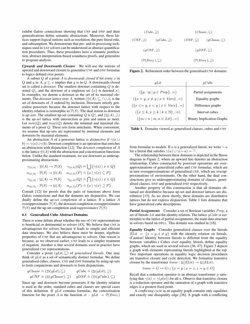
exhibit Galois connections showing that CNF and DNF and theirgeneralizations define semantic abstractions. Moreover, these lat-tices support logical notions such as resolution, the pure literal rule,and subsumption. We demonstrate that pre- and in-processing tech-niques used in SAT solvers can be understood as abstract quantifica-tion procedures. Thus, these procedures have a semantic justifica-tion, abstract interpretation-based soundness proofs, and generalizeto program analysis.

Upwards and Downwards Closure We will use the notions ofupward and downward closure to generalise CNF and DNF formulaeto logics defined over posets.

A subset Q of a poset A is downwards closed if for every x inQ and y in A, y v x implies that y is in Q. A downwards-closedset is called a downset. The smallest downset containing Q is de-noted Q�, and the downset of a singleton set {x} is denoted x�.In examples, we denote a downset as the set of its maximal ele-ments. The downset lattice over A, written (D(A),⊆,∩,∪), is theset of downsets of A ordered by inclusion. Downsets strictly gen-eralise powersets because the downset lattice with respect to theidentity relation is isomorphic to P(S). The dual notion to downsetis up-sets. The smallest up-set containing Q is Q�, and (U(A),⊇)is the up-set lattice with intersection as join and union as meet.Let min(Q) and max (Q) denote the minimal and maximal ele-ments of a poset Q. These sets form antichains. When convenient,we assume that up-sets are represented by minimal elements anddownsets by maximal elements.

An abstraction A of a powerset lattice is disjunctive if γ(a tb) = γ(a)∪γ(b). Downset completion is an operation that enrichesan abstraction with disjunction [12]. The downset completion of Ais the lattice D(A) with the abstraction and concretisation functionsbelow. Unlike the standard treatment, we use downsets as underap-proximating abstractions.

γD(A) : D(A)→ P(S) γD(A)(Q) =⋃{γ(x) | x ∈ Q}

αD(A) : P(S)→ D(A) αD(A)(P ) = {x | γ(x) ⊆ P}

γU(A) : U(A)→ P(S) γU(A)(Q) =⋂{γ(x) | x ∈ Q}

αU(A) : P(S)→ U(A) αU(A)(P ) = {x | γ(x) ⊇ P}Consult [12] for proofs that the pairs of functions above formGalois connections and that the domains are disjunctive. We candually define the up-set completion of a lattice. If a lattice Aoverapproximates P(S), the downset completion overapproximatesP(S) and the up-set completion underapproximates P(S).

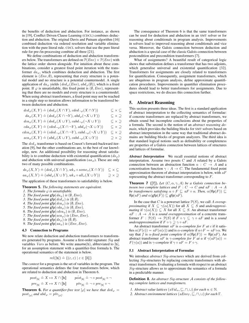
6.1 Generalised Cube Abstract DomainsThere is some debate about whether the use of CNF representationsis beneficial or detrimental to solvers [43]. We believe that CNF isadvantageous for solvers because it leads to simple and efficientdata structures. We also believe there must be deeper, algebraicproperties of CNF that are advantageous to solvers. One reason isbecause, as we observed earlier, CNF leads to a simpler treatmentof negation. Another is that several domains used in practice havegeneralized CNF representations.

Consider a poset (gLit ,v) of generalised literals. One maythink of gLit as a set of semantically distinct formulae. We definegeneralised cubes, clauses, CNF and DNF formulae by using up-setsto form conjunctions and downsets to form disjunctions.

gClause = (D(gLit),⊆) gCube = (U(gLit),⊇)

gCNF = (U(gClause),⊇) gDNF = (D(gCube),⊆)

Since up- and downsets become powersets if the identity relationis used as the order, standard cubes and clauses are special casesof this definition. If gLit contains formulae, the concretisationfunction for the poset A is the function st : gLit → P(EnvΓ)

(P(EnvΓ),⊆)

(gCNF ,⊇)

(CNF ,⊇) (gCube,⊇)

(Cube,⊇)

(P(EnvΓ),⊇)

(gDNF ,⊆)

(DNF ,⊆) (gClause,⊆)

(Clause,⊆)

Figure 2. Refinement order between the generalised CNF domains.

gLit gCube

({p,¬p | p ∈ Prop} ,=) Partial assignments

({x = y, x 6= y | x ∈ Vars} ,=) Equality graphs

({x <= y, x < y | x ∈ Vars} ,=) Difference graphs

({x ≤ k, x ≥ k | k ∈ N} ,⇒) Interval cubes

({m ∨ n |m,n ∈ Lit} ,=) Binary Implication Graphs

Table 1. Domains viewed as generalised clauses, cubes and CNF

from formulae to models. If a is a generalized literal, we write ∼ afor a literal that satisfies γ(a) ∪ γ(∼ a) = >.

The relationship between these domains is depicted in the Hassediagram in Figure 2, where an upward line denotes an abstractionrelationship. Cubes constructed by powerset operations are over-approximations of generalised cubes and CNF formulae, which arein turn overapproximations of generalised CNF, which are overap-proximations of environments. On the other hand, the dual con-structions give us underapproximating domains of clauses, gener-alised clauses, DNF and generalised DNF respectively.

Another property of this construction is that all domains ob-tained are distributive because up-set and downset lattices are dis-tributive [15]. As we show shortly, these domains are distributivelattices but do not express disjunction. Table 1 lists domains thathave generalized cube descriptions.

Partial Assignments Consider a set of Boolean variables Prop, aset of literals Lit and the identity relation. The lattice gCube is iso-morphic to the lattice of partial assignments, the main data structurein solvers based on DPLL. This domain was studied in [18].

Equality Graphs Consider generalized clauses over the literalsELit = {x = y, x 6= y} with the identity relation on literals.(Caution! Identity between literals is different from the equalitybetween variables.) Cubes over equality literals define equalitygraphs, which are used in several solvers [36, 47]. Figure 3 depictsa graph with elements representing literals highlighted at the top.Two important operations in equality logic decision proceduresare transitive closure and cycle detection. We formalize transitiveclosure by the transformer trans : U(ELit)→ U(ELit).

trans = G 7→ G ∪ {x = y | x = z, z = y ∈ G}Recall that a reduction operator is an abstract transformer ρ satis-fying that γ(a) = γ(ρ(a)) for all a. Observe that transitive closureis a reduction operator and the saturation of a graph with transitiveedges is a greatest fixed point.

A conflicting cycle in an equality graph contains only equalitiesand exactly one disequality edge [36]. A graph with a conflicting

disequality edgeequality edge

Figure 3. Equality graphs over three variables. The shaded ele-ments at the top are literals and the shaded elements at the bottomall concretise to the empty set.

cycle satisfies γ(G) = ∅. The shaded elements at the bottom ofFigure 3 all contain conflicting cycles and concretise to the emptyset. A similar abstract domain and reduction operation appear inthe logic of order and directed graphs in [31].

Interval Cubes Consider the set of single variable inequalities(BLit = {x ≤ k, x ≥ k | k ∈ Z} ,⇒). which form a poset un-der implication. The elements of BLit are light grey in Figure 4.By representing intervals as cubes instead of pairs, we obtain a set-based representation that supports proof rules such as resolutionand other algorithms in solvers that target clauses and cubes. Ex-ample 6 illustrates how intervals can be manipulated using up-sets.Example 6. The interval domain as defined in Section 5 is notdistributive because identities such as the one below fail.

([0, 1] t [6, 7]) u [3, 4] = [3, 4]

6= ([0, 1] u [3, 4]) t ([6, 7] u [3, 4]) = ⊥Now consider intervals represented as up-sets. The meet in thislattice is union and join is intersection, so it is trivially distributive.We represent up-sets by their minimal elements.

({x ≥ 0, x ≤ 1} � ∩ {x ≥ 6, x ≤ 7} �) ∪ {x ≥ 3, x ≤ 4} �= {x ≥ 0, x ≤ 7} � ∪ {x ≥ 3, x ≤ 4} � = {x ≥ 3, x ≤ 4} �

A similar calculation yields the expected interval for the otherinterval expression. The cube representation expresses the sameconcrete elements as the classic pair representation of intervals butcontains more redundancy. C

Binary Implication Graphs If the set of generalised literals con-tains clauses of length 2 (such as {p,¬q}) ordered by equality, eachgeneralised literal represents two implications q ⇒ p and ¬p⇒ q,which can be viewed as edges in a directed graph. The resultingBinary Implication Graph abstract domain is used for preprocess-ing in SAT solvers [29]. Though a lattice-based analysis has notbeen previously applied to Binary Implication Graphs, we need notexplicitly define Galois connections or their approximation proper-ties, as these follow from the cube representation. As with equalitygraphs, transitive closure is a reduction.

The CNF Domains The generalized CNF domains show that CNFformulae have a lattice structure that is usually not recognized. Tosee the difference between gCNF and CNF , consider BLit . Theset {x ≥ 2, x ≤ 5, x ≤ 7} represents a clause but not a generalizedclause, while {x ≥ 2, x ≤ 5} � is a generalised clause.

Solvers use a variety of subsumption techniques to minimizeformulae without explicitly checking implication. The inclusion

>

〈x < 100〉

〈x < 99〉

〈y < 100〉

〈y < 99〉

〈x ≥ 0〉

〈x ≥ 1〉

〈y ≥ 0〉

〈y ≥ 1〉

〈x : [1, 98]〉〈x < 99, y < 99〉 〈x ≥ 1, y ≥ 1〉

〈x : [3, 9], y : [1, 6]〉〈x : [3, 7], y : [1, 4]〉 〈x : [7, 9], y : [4, 6]〉

〈x : 3, y : 1〉 〈x : 7, y : 4〉 〈x : 9, y : 6〉

⊥

Figure 4. The lattice of interval environments over two variables.The shaded elements at the top represent the poset of literals whileelements at the bottom represent singleton values.

orders in Figure 2 correspond to subsumption notions and alsounderapproximate implication. For instance, {{p} , {p, q}} and{{p}} are logically equivalent but we can only show {{p}} ⊆{{p} , {p, q}} using the lattice order. From the abstract interpreta-tion perspective, subsumption is not a substitute for implication butis fundamental to the lattice structure of CNF and DNF domains.

6.2 Abstract Transformers in SolversGeneralized Unit Rule The unit rule in SAT solvers asserts that ifa cube represents a region of the search space and the cube falsifiesall but one literal in a clause, the remaining literal can be addedto the clause. The Abstract Conflict Driven Learning algorithm(ACDCL) of [19] generalises the unit rule to abstract domains basedon the notion of complementable meet irreducibles. The unit rulecan be viewed as a technique for refining generalized cubes usinggeneralized clauses.

gunit : gClause → (gCube → gCube)

gunitθ = π 7→ π ∪ {a} , where a ∈ θ, γ(π) ∩ γ(a) 6= ∅, andfor all b ∈ θ \ {a} , γ(π) ∩ γ(b) = ∅

We write gfpx(f) for the function that maps elements a to fixedpoints gfp(f(a, x)) of a function f(y, x). The main observationof [18] was that Boolean Constraint Propagation (BCP) is a fixedpoint bcp(ϕ, x) = gfpx(

dθ∈ϕ gunitθ) defined pointwise over unit

rules. The generalized cubes in Table 1, when combined with thegeneralized clauses, also support the unit rule and BCP.

Failed Literal Probing Failed literal probing [21, 22] is a prepro-cessing technique in SAT solvers. The technique chooses literal a,computes bcp(a, ϕ) and if the result is⊥, adds the singleton clause{b} to ϕ, where b satisfies that γ(a)∪γ(b) = >. No action is takenif the result is not bottom. Note that we have not only describedfailed literal probing, but also its generalization to CNF domains.

Clause Dropping Variable elimination is a fundamental opera-tion underlying quantifier elimination, deduction and syntactic sim-plification of formulae. The simplest form of sound variable elim-ination is to drop clauses from a CNF formula in which the targetvariable occurs. This idea lifts directly to generalized CNF domainsif we drop constraints based on the literals they contain.

drop : gLit × gCNF → gCNF

dropp(ϕ) = {C | {p,∼ p} ∩ C = ∅, C ∈ ϕ}In general, dropp is an overapproximation of the deduction trans-former. If p is a Boolean variable, dropp also overapproximatesexistential quantification with respect to p.

Resolution The resolution principle asserts that if C ∨ p and¬p∨D are both satisfiable, so is C ∨D. The variable p is the pivotand C ∨ D is the resolvent. Generalised CNF domains support ageneralization of resolution res : gLit × gCNF → gCNF .

res(p, ϕ) = {C ∪D | C ∪ {p} , D ∪ {q} ∈ ϕ, γ(p) ∩ γ(q) = ∅}

Generalized CNF domains that apply this transformer can produceresolution-style proofs, which is a first step towards combiningexisting abstract domains with proof-theoretic techniques.Example 7. The generalised CNF element

ϕ = {{x ≥ 10, x ≤ 5} �, {x ≥ 7, x ≤ 13} �}

represents a conjunction of disjunctions of bounds. Standard inter-val propagation will lose precision in the clauses, while standardresolution does not apply because no constraint is the negation ofanother. The result of generalized resolution with respect to the lit-eral x ≥ 7 is res(x ≥ 7, ϕ) = {{x ≥ 10, x ≤ 13}}. Thougharithmetic techniques methods can deduce the same information,generalised resolution is simple and suffices in this case. C

The Pure Literal Rule Clause dropping is a sound but incompletesimplification technique because a formula ϕ that is unsatisfiablemight become satisfiable after clause dropping. The pure literalrule, introduced in the original algorithm of Davis and Putnam [16]can be understood as an application of clause dropping only insituations where it does not change the satisfiability of a formula.We formalize the pure literal rule for generalized CNF domains.

Recall that gLit is the set of generalized literals. We say thata set of literals A is pure if for each a in A, no b satisfyingγ(a) ∩ γ(b) = ∅ is also in A. We assume that gLit is the disjointunion of two pure sets P and N such that for each a in P , thereexists a b in N satisfying that γ(a)∩ γ(b) = ∅ and vice-versa. Theelements of P are positive literals and of N are negative literals.Define a set {+,−} of polarities, a lattice of polarities P({+,−}),and a lattice of polarity maps P → P({+,−}).

Polarity analysis of a generalized CNF formula ϕ computes apolarity map ρ. such that ρ(`) is {+} or {−} if the generalizedliteral ` only occurs positively or only negatively in ϕ, and is ∅ if `does not occur in ϕ, and is {+,−} if ` occurs both positively andnegatively in ϕ. The polarity of a literal ` is {+} if a is in P , andis {−} if ` is in N . The polarity map for a literal ` sends ` to itspolarity and sends all literals b 6= a to the empty set. The polaritymap for a generalized clause is the pointwise join of of polaritymaps of its literals. The polarity map of a generalized CNF elementis the pointwise join of of polarity maps of its clauses. Note that thejoin is used in both cases.

The pure literal rule for a generalized CNF formula, appliesdrop` to a formula ϕ only if the polarity map for ϕ does not sendthe literal ` to {+,−}. The pure literal rule is a sound overapprox-imation of the deduction transformer and is a refinement of clausedropping. In propositional logic, the pure literal rule applied to avariable p is also a sound abstraction of the existential quantifica-tion transformer (wkp ◦ somep).

7. Discussion and Related WorkThis paper contributes to a research programme that seeks to closethe gap between abstract interpretation techniques and deductionalgorithms, both in theory and practice. One direction of this pro-gram is to use deduction algorithms to refine static analyses. Pre-cision loss due to joins was reduced by boosting a static analysiswith unification [46], DPLL(T) [27], or CDCL [20]. Best abstracttransformers have been synthesized using satisfiability solvers [41],and Stalmarck’s method [45], while [37] applied satisfiability tech-niques to reduce precision loss in fixed point iteration.

Another direction in this programme is to characterize satisfi-ability procedures as abstract interpretations. Boolean constraintpropagation was shown to be an abstract interpretation in [18], andCDCL was generalized to combine deduction and abduction overlattices in [19]. Stalmarck’s method was characterized as a tech-nique for refining abstract transformers in [44]. The Nelson-Oppenmethod for theory combination implemented in SMT solvers wasshown to be a special case of the reduced product of abstract do-mains [14]. The DPLL(T) technique for reasoning about a theory bycombining a SAT solver with a theory solver was also shown to bea special case of the reduced product in [2].

In addition to static analysis applications, these characteriza-tions provide a new way for lifting solver algorithms to new logics.For example, Stalmarck’s method was lifted to arithmetic in [45],while CDCL was lifted to floating point logic in [26]. Note thatthe Nelson-Oppen combination was lifted to abstract domains [25]prior to the reduced product characterization.

Abstract satisfaction is lattice-theoretic in an attempt to alignwith static analysis. If static analysis is ignored, the DPLL(T) frame-work provides one generic approach to implementing decision pro-cedures [23]. The separation of Boolean and theory reasoning inDPLL(T) can be detrimental to performance and has driven thesearch for other frameworks. Abstract DPLL [39], natural domainSMT [6], generalized DPLL [35], and the model construction calcu-lus [17] are attempts in this direction.

8. ConclusionAbstraction is fundamental to practical reasoning about computa-tionally intractable problems. Abstract interpretation has tradition-ally been applied to reason about undecidable problems such aschecking semantic properties of programs. This paper introduced aframework for applying abstract interpretation to problems that areNP-hard but decidable, such as satisfiability.

This framework allows for novel perspectives of SMT algo-rithms. Solvers can be viewed as abstract interpretation portfo-lios, which combine several different, weak abstractions to achievea conclusive result. Moreover, while solvers use incomplete ab-stractions they produce complete results. This is not due to brute-force enumerations but clever, semantics-based refinement tech-niques. Our framework makes some of these techniques explicit,but more importantly provides a general vocabulary for studying awide range of satisfiability procedures.

While the focus of this paper has been theoretical, our goal isto contribute to the practical state of the art. The original abstractinterpretation framework provided a simple recipe for constructingstatic analyzers. Abstract satisfaction plays a similar role and pro-vides a foundation for the development of programmable, lattice-based SMT solvers.

There are three different axes for future work. One is to ap-ply abstract interpretation to the implementation of SMT solvers byconstructing sound but incomplete solvers and abstract quantifica-tion procedures from existing abstract domains. The second axis isto lift techniques in SMT solvers to improve the precision and effi-ciency of program analysis. The classic DPLL, DPLL(T), CDCL andStalmarck’s method have each been lifted to a single static analy-sis problem, but more applications and evaluation are required tounderstand their strengths in a static analysis context. Preprocess-ing, subsumption, and sparsity techniques have all been integral toimproving the performance of solvers, and the connections in thispaper indicate that such techniques should lift to program analy-sis as well. The final axis is to investigate new implementations ofabstract domains with interfaces rich enough to support SMT solv-ing, static analysis, implication graph construction, and domain andtheory combinations. We look forward to these developments.

AcknowledgmentsThis work was supported by the Toyota Motor Corporation, ERCproject 280053, EPSRC project EP/H017585/1, and the FP7 STREPPINCETTE. The research reported in this paper was conducted be-tween 2011 and 2013. In 2011, Vijay D’Silva was supported by aMicrosoft Research scholarship.

References[1] N. Bjørner, B. Duterte, and L. de Moura. Accelerating lemma learning

using joins – DPLL(t). In LPAR, 2008.

[2] M. Brain, V. D’Silva, L. Haller, A. Griggio, and D. Kroening. Anabstract interpretation of DPLL(T). In VMCAI, 2012.

[3] M. Brain, V. D’Silva, L. Haller, A. Griggio, and D. Kroening.Interpolation-based verification of floating-point programs with ab-stract CDCL. In SAS, 2013.

[4] R. E. Bryant, D. Kroening, J. Ouaknine, S. A. Seshia, O. Strichman,and B. Brady. Deciding bit-vector arithmetic with abstraction. InTACAS, pages 358–372. Springer, 2007.

[5] E. M. Clarke, O. Grumberg, and D. E. Long. Model checking andabstraction. ACM TOPLAS, 16(5):1512–1542, Sept. 1994.

[6] S. Cotton. Natural domain SMT: A preliminary assessment. InFORMATS, pages 77–91, 2010.

[7] P. Cousot. Semantic foundations of program analysis. In S. Muchnickand N. Jones, editors, Program Flow Analysis: Theory and Applica-tions, chapter 10, pages 303–342. Prentice-Hall, Inc., 1981.

[8] P. Cousot. The calculational design of a generic abstract interpreter. InM. Broy and R. Steinbruggen, editors, Calculational System Design.NATO ASI Series F. IOS Press, Amsterdam, 1999.

[9] P. Cousot. Abstract interpretation. MIT course 16.399, 2005.

[10] P. Cousot and R. Cousot. Abstract interpretation: a unified latticemodel for static analysis of programs by construction or approxima-tion of fixpoints. In POPL, pages 238–252. ACM Press, 1977.

[11] P. Cousot and R. Cousot. Systematic design of program analysisframeworks. In POPL, pages 269–282. ACM Press, 1979.

[12] P. Cousot and R. Cousot. Abstract interpretation and application tologic programs. Journal of Logic Programming, 13(2–3):103–179,1992.

[13] P. Cousot and R. Cousot. Abstract interpretation frameworks. Journalof Logic and Computation, 2(4):511–547, Aug. 1992.

[14] P. Cousot, R. Cousot, and L. Mauborgne. Theories, solvers and staticanalysis by abstract interpretation. JACM, 59(6):31:1–31:56, Jan.2013.

[15] B. A. Davey and H. A. Priestley. Introduction to lattices and order.Cambridge University Press, Cambridge, UK, 1990.

[16] M. Davis and H. Putnam. A computing procedure for quantificationtheory. JACM, 7:201–215, July 1960.

[17] L. M. de Moura and D. Jovanovic. A model-constructing satisfiabilitycalculus. In VMCAI, pages 1–12, 2013.

[18] V. D’Silva, L. Haller, and D. Kroening. Satisfiability solvers are staticanalysers. In SAS, pages 317–333. Springer, 2012.

[19] V. D’Silva, L. Haller, and D. Kroening. Abstract conflict drivenlearning. In POPL, pages 143–154, New York, NY, USA, 2013. ACMPress.

[20] V. D’Silva, L. Haller, D. Kroening, and M. Tautschnig. Numericbounds analysis with conflict-driven learning. In TACAS, pages 48–63. Springer, 2012.

[21] N. Een and A. Biere. Effective preprocessing in SAT through variableand clause elimination. In SAT, pages 61–75, Munich, Germany, 2005.Springer.

[22] J. W. Freeman. Failed literals in the Davis-Putnam procedure for SAT.Technical report, Rutgers University, 1993.

[23] H. Ganzinger, G. Hagen, R. Nieuwenhuis, A. Oliveras, and C. Tinelli.DPLL(T): Fast decision procedures. In CAV, pages 175–188, 2004.

[24] R. Giacobazzi, F. Ranzato, and F. Scozzari. Making abstract interpre-tations complete. JACM, 47(2):361–416, 2000.

[25] S. Gulwani and A. Tiwari. Combining abstract interpreters. In PLDI,pages 376–386. ACM Press, 2006.

[26] L. Haller, A. Griggio, M. Brain, and D. Kroening. Deciding floating-point logic with systematic abstraction. In FMCAD, pages 131–140,2012.

[27] W. R. Harris, S. Sankaranarayanan, F. Ivancic, and A. Gupta. Programanalysis via satisfiability modulo path programs. In POPL, pages 71–82, 2010.

[28] T. A. Henzinger, O. Kupferman, and S. Qadeer. From pre-historic topost-modern symbolic model checking. FMSD, 23(3):303–327, Nov.2003.

[29] M. J. H. Heule, M. Jarvisalo, and A. Biere. Efficient CNF simplifi-cation based on binary implication graphs. In SAT, pages 201–215,2011.

[30] D. Kroening, J. Ouaknine, S. A. Seshia, and O. Strichman.Abstraction-based satisfiability solving of Presburger arithmetic. InCAV, pages 308–320, July 2004.

[31] D. Kroening and G. Weissenbacher. An interpolating decision pro-cedure for transitive relations with uninterpreted functions. In HVC,pages 150–168, 2011.

[32] W. Lawvere. Adjointness in foundations. Dialectica, 23:281–296,1969.

[33] K. R. M. Leino and F. Logozzo. Using widenings to infer loopinvariants inside an SMT solver, or: A theorem prover as abstractdomain. In Workshop on Invariant Generation, pages 70–84. RISCReport 07-07, 2007.

[34] K. L. McMillan. Interpolation and SAT-based model checking. InCAV, pages 1–13, 2003.

[35] K. L. McMillan, A. Kuehlmann, and M. Sagiv. Generalizing DPLL toricher logics. In CAV, pages 462–476, 2009.

[36] O. Meir and O. Strichman. Yet another decision procedure for equalitylogic. In CAV, pages 307–320, 2005.

[37] D. Monniaux and L. Gonnord. Using bounded model checking tofocus fixpoint iterations. In SAS, pages 369–385, 2011.

[38] I. Nemeti. Algebraization of quantifier logics, an introductoryoverview. Studia Logica: An International Journal for Symbolic Logic,50(3/4):485–569, 1991.

[39] R. Nieuwenhuis, A. Oliveras, and C. Tinelli. Solving SAT andSAT modulo theories: From an abstract Davis–Putnam–Logemann–Loveland procedure to DPLL(T). JACM, 53:937–977, 2006.

[40] A. M. Pitts. Categorical logic. In S. Abramsky, D. M. Gabbay, andT. S. E. Maibaum, editors, Handbook of Logic in Computer Science,Volume 5. Algebraic and Logical Structures, chapter 2, pages 39–128.Oxford University Press, 2000.

[41] T. W. Reps, S. Sagiv, and G. Yorsh. Symbolic implementation of thebest transformer. In VMCAI, pages 252–266, 2004.

[42] P. Smith. The Galois connection of syntax and semantics. Technicalreport, Cambridge University, 2010.

[43] P. J. Stuckey. There are no CNF problems. SAT, pages 19–21, 2013.[44] A. Thakur and T. Reps. A generalization of Stalmarck’s method. In

SAS. Springer, 2012.[45] A. V. Thakur and T. W. Reps. A method for symbolic computation of

abstract operations. In CAV, 2012.[46] A. Tiwari and S. Gulwani. Logical interpretation: Static program

analysis using theorem proving. In CADE, pages 147–166, 2007.[47] O. Tveretina. DPLL-based procedure for equality logic with unin-

terpreted functions. In IJCAR Doctoral Programme, volume 106 ofCEUR Workshop Proceedings. CEUR-WS.org, 2004.